Hybrid Computational Intelligence Models for Improvement Gully Erosion Assessment


1
Department of Geomorphology, Tarbiat Modares University, Jalal Ale Ahmad Highway, Tehran 9821, Iran
2
Key Laboratory of Coal Resources Exploration and Comprehensive Utilization, Ministry of Natural Resources, Xi’an 710021, China
3
College of Geology and Environment, Xi’an University of Science and Technology, Xi’an 710054, China
4
Shaanxi Provincial Key Laboratory of Geological Support for Coal Green Exploitation, Xi’an 710054, China
5
Faculty of Geo-Information Science and Earth Observation (ITC), University of Twente, Drienerlolaan 5, 7522 NB Enschede, The Netherlands
6
Department of Geoinformatics—Z_GIS, University of Salzburg, Salzburg 5020, Austria
7
Institute of Research and Development, Duy Tan University, Da Nang 550000, Vietnam
*
Authors to whom correspondence should be addressed.
Remote Sens. 2020, 12(1), 140; https://0-doi-org.brum.beds.ac.uk/10.3390/rs12010140
Submission received: 12 November 2019
/
Revised: 5 December 2019
/
Accepted: 27 December 2019
/
Published: 1 January 2020
(This article belongs to the Special Issue Advanced Machine Learning Techniques for High-Resolution Remote Sensing Data Analysis)
Abstract
:Gullying is a type of soil erosion that currently represents a major threat at the societal scale and will likely increase in the future. In Iran, soil erosion, and specifically gullying, is already causing significant distress to local economies by affecting agricultural productivity and infrastructure. Recognizing this threat has recently led the Iranian geomorphology community to focus on the problem across the whole country. This study is in line with other efforts where the optimal method to map gully-prone areas is sought by testing state-of-the-art machine learning tools. In this study, we compare the performance of three machine learning algorithms, namely Fisher’s linear discriminant analysis (FLDA), logistic model tree (LMT) and naïve Bayes tree (NBTree). We also introduce three novel ensemble models by combining the aforementioned base classifiers to the Random SubSpace (RS) meta-classifier namely RS-FLDA, RS-LMT and RS-NBTree. The area under the receiver operating characteristic (AUROC), true skill statistics (TSS) and kappa criteria are used for calibration (goodness-of-fit) and validation (prediction accuracy) datasets to compare the performance of the different algorithms. In addition to susceptibility mapping, we also study the association between gully erosion and a set of morphometric, hydrologic and thematic properties by adopting the evidential belief function (EBF). The results indicate that hydrology-related factors contribute the most to gully formation, which is also confirmed by the susceptibility patterns displayed by the RS-NBTree ensemble. The RS-NBTree is the model that outperforms the other five models, as indicated by the prediction accuracy (area under curve (AUC) = 0.898, Kappa = 0.748 and TSS = 0.697), and goodness-of-fit (AUC = 0.780, Kappa = 0.682 and TSS = 0.618). The analyses are performed with the same gully presence/absence balanced modeling design. Therefore, the differences in performance are dependent on the algorithm architecture. Overall, the EBF model can detect strong and reasonable dependencies towards gully-prone conditions. The RS-NBTree ensemble model performed significantly better than the others, suggesting greater flexibility towards unknown data, which may support the applications of these methods in transferable susceptibility models in areas that are potentially erodible but currently lack gully data.
1. Introduction
In the last two decades, computational capacity and methodological development have improved significantly in all branches of science dealing with predictive modeling [1]. Geomorphology has experienced technological advancements in two ways. The first was the creation of geographic information systems (GIS), which started as a means to managing spatial data and gradually became a fundamental tool for planning [2], visualizing and communicating [2] in geoscience.
The second major advancement was the implementation of predictive/susceptibility models [3]. The GIS structure enabled very early or even pioneering studies via bivariate models [4]. These models, and all their proposed variations, essentially boil down to the calculation of relative frequencies of geomorphological processes, be they landslides [5], or gullies [6], within specific portions of preconditioning factors’ domains. These frequencies are used to derive weights describing the associations between a given hazard and predisposing factors, and, ultimately, the spatial susceptibility distribution [7]. Bivariate models are very convenient as the required calculations are so simple that they can be entirely made within any GIS [8]. However, despite their simplicity, bivariate models have also proved to have good predictive performance and support clear geomorphological interpretation [9].
Nevertheless, most of the proposed bivariate models do not strictly rely on an underlying probability distribution [10,11], which makes multivariate statistical approaches more suited to assessing the susceptibility of a given region. The generalized linear models (GLMs) [11], where the underlying probability distribution corresponds to the Bernoulli exponential family [12], are the most commonly applied multivariate applications in geomorphology. As a result, GLMs rely on more rigorous statistical assumptions, provide good performances compared to multivariate models and allows for interpreting linear effects of the given set of predisposing factors [13]. An extension to this paradigm is the so-called generalized additive models (GAMs) [14], in which the algorithmic structure remains the same as in the GLMs but allows for testing nonlinear effects of each predisposing factors [15].
Pourghasemi and Rossi [16] mention that multivariate models have largely dominated the literature in the last decade. However, during the same period, machine learning tools proved to be an even better alternative to multivariate models for susceptibility analysis with greater performance reported in many comparative studies [17]. Greater performance being reported due to the different way in which machine learning approaches model natural hazards and their association with predisposing factors. For instance, decision trees, and their proposed variations all share a common feature. They slice each predisposing factors’ domain in successive halves and derive data-driven rules to differentiate between stable and unstable conditions [18]. However, the high performance in terms of modeling is reached by sacrificing the interpretability of the model results. In fact, machine learning tools only provide a measure of how much variability in the data is explained by a given factor, which is commonly known as predictor importance [19]. The high performances in terms of modeling may also be affected by overfitting issues.
To overcome the overfit, an even more recent approach has been proposed and tested, namely ensemble modeling [20]. Ensembles are combinations of several predictive models into a single model. The summary of different outputs can be generally expressed as the mean, or another aggregative measure, of the various models. It guarantees that the large differences resulting from several different model structures are smoothed out, leaving the common pattern where either high or low susceptibility estimates have been recognized through multiple approaches of the different models [21].
In this work, we tested the most recent trend in susceptibility modeling by considering the predictive performances of three machine learning algorithms namely, Fisher’s linear discriminant analysis (FLDA), logistic model tree (LMT), naïve-Bayes tree (NBTree) and their corresponding ensemble with a Random SubSpace (RS, Barandiaran, 1998). In a nested experiment, we also adopted an evidential belief function (EBF) [22] to assess the predisposing factors’ effects. The purpose of this study was to model gully erosion-prone areas in Iran. Approximately 76% of Iran is affected by water-driven erosion, and widespread gullying has been reported in almost the entire nation, from the south [23] to the north [24] and from the west [25] to the central provinces [26], leaving only the easternmost sectors of the country less affected. The combined effect of water erosion is responsible for permanently washing away one millimeter of soil per year across the whole country. For this reason, a national-wide effort is currently being coordinated by local research institutions to study erosional processes and plan mitigation/remediation actions. Of the erosion processes, gullying is one of the most evident in the short-term and also one of the most prominent examples of how dangerous soil loss can be, especially in arid to semi-arid environments. In such geographic settings, a single gully can extend vertically for several meters and horizontally up to several hundred meters [9]. In coordination with the national effort, we focus on the Toroud watershed, where 129 gullies have been recently reported. This area was still untested despite the worrying number of gullies, and we opted to investigate it via state-of-the-art machine learning approaches. The manuscript is organized as follows: Section 2 introduces the study area; Section 3.1 and Section 3.2 provide a description of the gully phenomena and the predisposing factors we selected; Section 3.3 describe the predictive models used in this work and ultimately Section 4 report the results, their interpretation and the concluding remarks, respectively.
2. Materials and Methods
2.1. Study Area
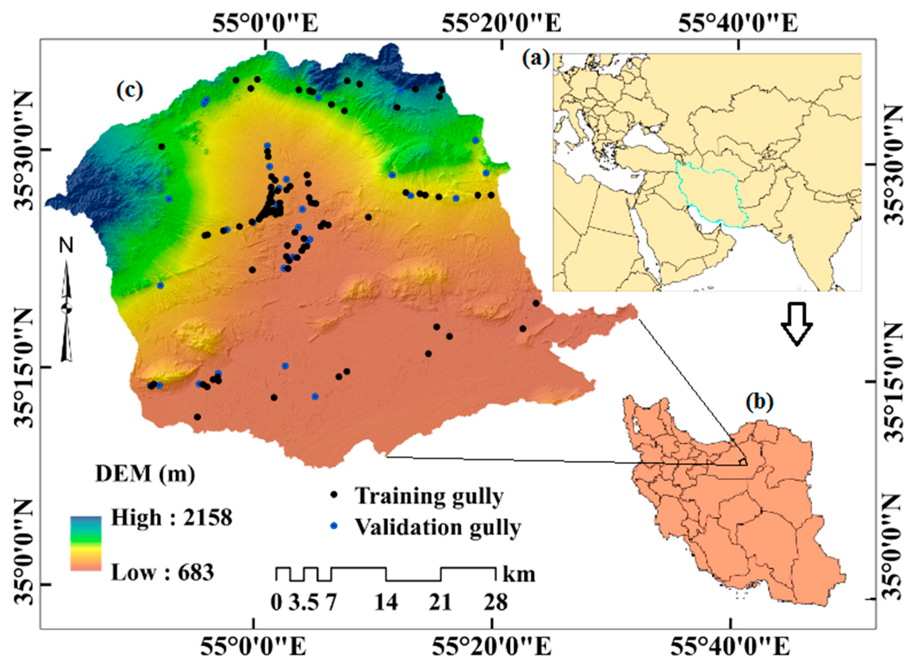
The study area lies within the Semnan province in Iran, and it is centered at approximately 35°26′10″N and 55°06′44″ (Figure 1). It covers a relatively small area of approximately 2400 km2, where the maximum variation in elevation is in the NE–SE axis. Specifically, the average altitude in the NE part is 2160 m.a.s.l., while in the SE it is 680 m.a.s.l. Since the catchment is relatively small, the associated slope significantly varies between flat conditions and 70°, but the average steepness is approximately 3 degrees. Due to the predominantly flat conditions, water stagnation prevails rather than runoff, which is generally the case under the local meteorological conditions responsible for a mean yearly discharge confined to between 48 and 206 mm during the wet season from January to March [27]. The associated temperature regimes reach a peak of 42 °C during summer, especially in the South. It decreases to below 0 °C during winter, towards the Northern regions. The temperatures during the rest of the year range from 14 °C to 24 °C. Overall, these are already indicators of meteorological stress with high variations and local spikes. This may generate freezing and thawing processes in soils as well as expansion and contractions also in the soils, which in turn can open cracks along the regolithic profile.
The local land cover encompasses agricultural fields, bare land, kavir, poorrange, rock outcrops, a salt lake, wetlands and salt lands. The latter are particularly vulnerable to dissolution processes during the wet season as the salt crust is easily chemically weathered, giving rise to pores, which promote water fluxes and associated erosion within soils. The distribution of these salt crusts is much more evident in the soil map (primarily featuring Aridisol and Entisols) and where the outcropping lithologies are also reported. The outcropping lithotypes [28] include: Quaternary sediments, comprising Qft1 (High-level piedmont fan and valley terrace deposits), Qft2 (Low-level piedmont fan and valley terrace deposits), Qsl (salt lake) Qsf (Salt flat) and Jurassic sediments, comprising Jph (phyllite, slate and meta-sandstone (Hamadan phyllites) and Jdav (Jurassic dacite to andesite lava flows).
2.2. Data Collection
2.2.1. Gully Phenomena and Inventory Map
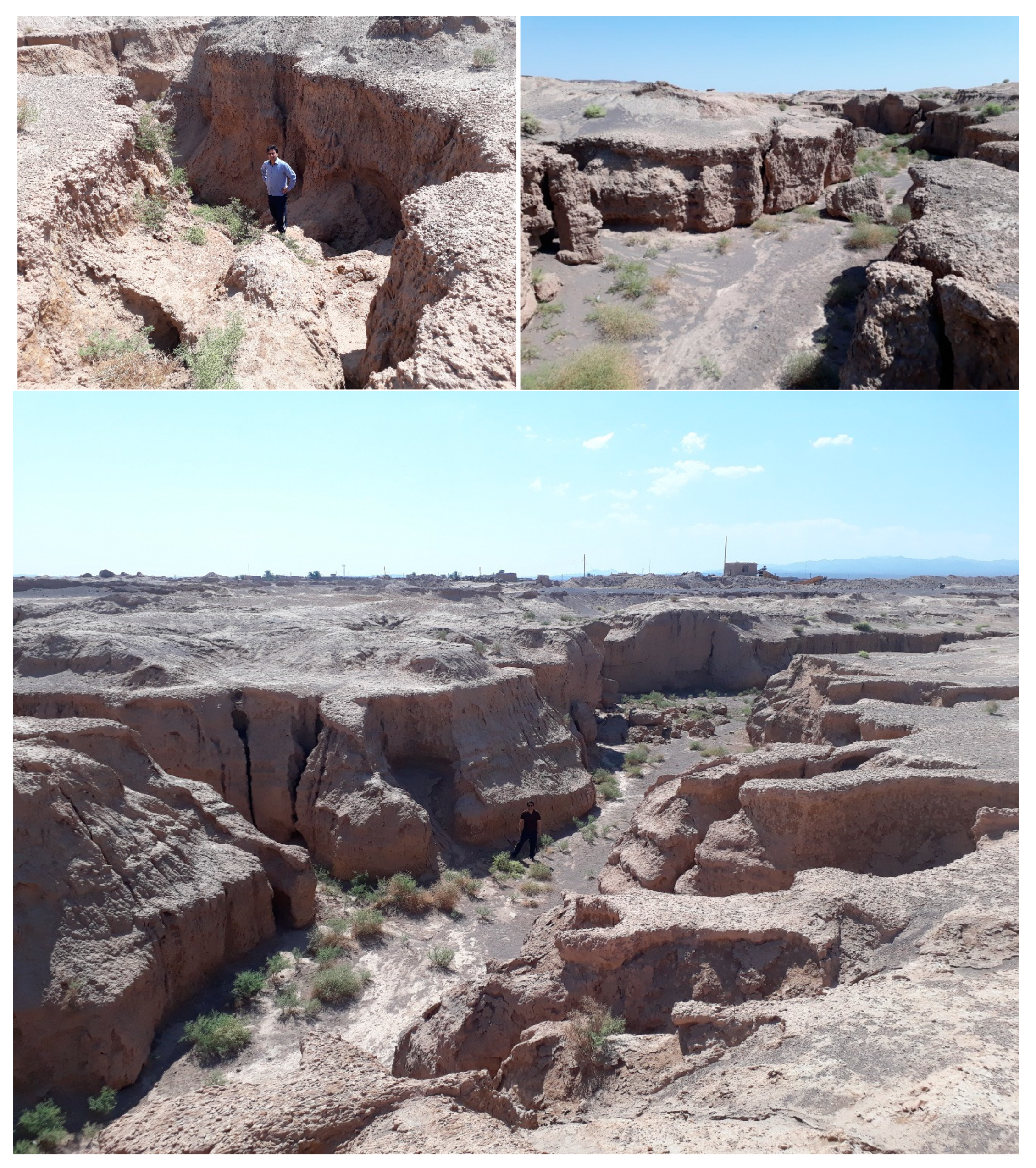
The target variable we want to model needs to be digitally represented in a gully erosion inventory map (GEIM), where the spatial distribution of gullies is reported. To generate the GEIM for the present study area, we initially accessed the archive compiled by the Isfahan Agricultural and Natural Resources, Research and Education Center (http://esfahan.areeo.ac.ir/). This information represents the foundation upon which we investigated the historical reports of gully occurrences. Upon which we organized our field and remote mapping procedures to update and refine the inventory. Specifically, we visited the sites (see Figure 2) for precise mapping via GPS (global positioning system) ground points measured at the gully head-cuts; whereas, for a broader view of the area, we used Google Earth to map the gully extents. Overall, we mapped a total of 129 gully head-cuts, which we then used during the modeling procedure as the target variable to be fitted and predicted. Specifically, we fitted each of the implemented models with 90 head-cuts (70%) and predicted the complementary 39 gully occurrences (30%). Some of mapped gullies in the study area are shown in Figure 2. However, as the selection of models corresponds to a presence–absence type, we randomly selected an equal number of absence locations. In turn, this procedure creates a balanced dataset for the subsequent analyses. However, it should be noted that the geomorphological community still debates on whether balanced [9] or unbalanced [15] datasets should be built prior to any susceptibility analysis.
2.2.2. Predisposing Factors
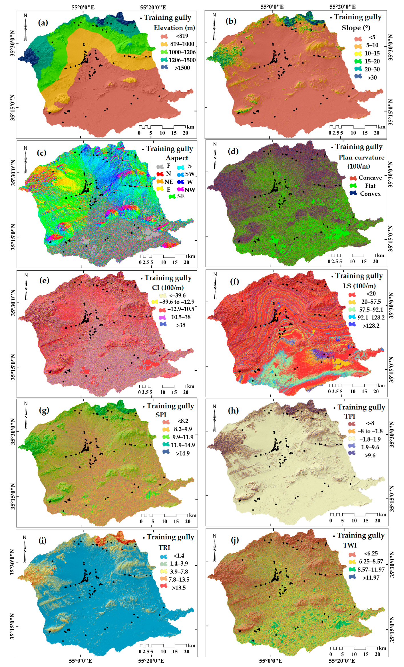
From an original DEM (digital elevation model) acquired from ALOS (advanced land observing satellite), with 12.5 m resolution, we derived a set of morphometric properties to describe the geomorphology of the area. Specifically, we extracted a series of DEM derivatives and combined them into a set of thematic properties that we either directly accessed from local territorial institutions, or computed. These are listed in Table 1 and shown in Figure 3.
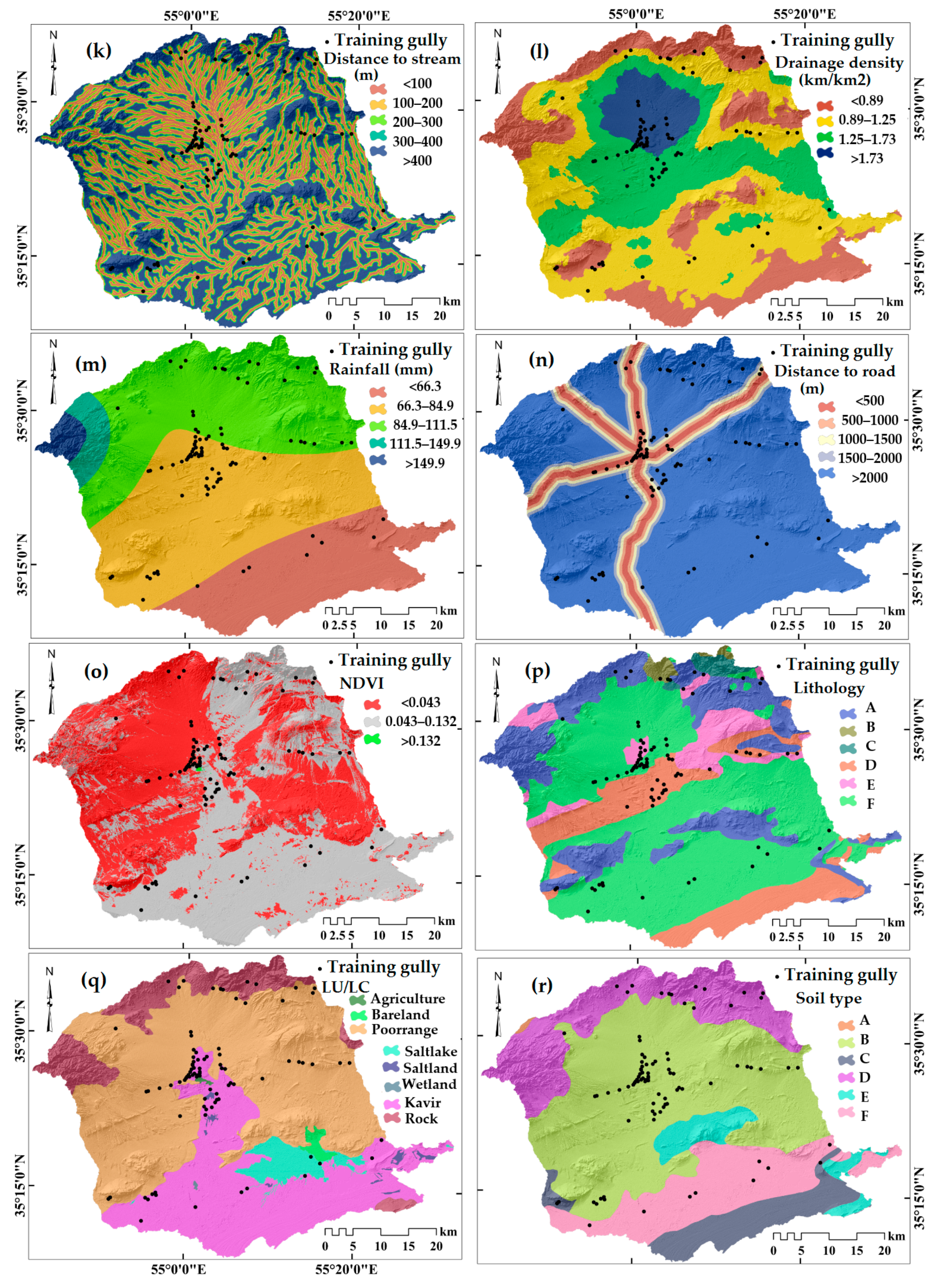
In addition to the morphometric factors, we computed hydrologically oriented properties such as drainage density, which is defined as the total stream length divided by the area of a moving circular neighborhood; the distance to stream, defined as the Euclidean distance from each pixel to the nearest stream line and rainfall, which was provided by the Iran meteorological organization, see [27]. To estimate the anthropic effects of overland flows, we computed the distance to road as the Euclidean distance from each pixel to the nearest road. The effect of vegetation on water absorption was accounted for using the NDVI (normalized difference vegetation index) obtained from a LANDSAT 8 (2018/08/12) scene of the area. The land use/cover was obtained from a supervised classification of the spectral properties obtained by LANDSAT 8. Lithology was digitized from the local geological map at 1: 100,000 scale, see GSDI (1997) for the original map. A description of the lithology units in the study area is given in Table 2. The soil type was digitized from the soil map provided by the soil conservation section of agricultural and natural resources research center of Semnan province.
2.3. Multicollinearity Assessment
Although machine learning algorithms do not strictly require the elimination of redundant conditioning factors, any predictive algorithm benefits from removing collinear properties [29]. Furthermore, in this work, we also focus on interpreting predisposing factors’ effects, so checking whether the signal carried by one property is linearly linked to another helps to disregard interdimensional relations before they can affect the models, which would disrupt the interpretation through confounding effects. Consequently, we included a test for multicollinearity in our workflow. The criterion we opted for includes two metrics, namely tolerance (TOL) and the variance inflation factor (VIF) [30,31,32].
Regarding the TOL, values equal to or lower than 0.1 indicate a potential collinearity issue of a specific conditioning factor. Similarly, a VIF ≥ 10 confirms the same numerical indication. We calculated the two metrics mentioned above for each continuous property, leaving aside the categorical ones (land use/cover, lithology and soil type). We reported the results of the multicollinearity tests in Table 3, where no factor appears to be linearly related to the others. Having ensured that no multicollinearity affects the factor set we initially chose, we post-processed each layer by reclassifying it into a number of sub-classes. We opted for a binning procedure based on the natural break method [33,34]. The reclassified rasters and the three categorical ones represent the factor set we subsequently explored for associations with respect to gully occurrences, as well as for the susceptibility mapping procedures, as detailed in the following sections.
2.4. Models
2.4.1. Predisposing Factors’ Effects Via EBF Model
We assessed the spatial dependence of gully locations on the selected predisposing factors via the EBF. We chose this method because of its straightforward interpretability and because it has been previously tested in several other susceptibility applications [9]. The theoretical foundations of EBF can be found in the Dempster–Shafer theory of evidence [35,36]. The full implementation of EBF relies on four components or belief functions, namely belief (Bel), disbelief (Dis), uncertainty (Unc) and plausibility (Pls). For susceptibility mapping purposes, all four components need to be computed and aggregated [9]. However, here we chose to use EBF solely as an explanatory tool by only focusing on the Bel function as this component alone allows one to interpret a factors’ effects on a binary target variable. We implemented EBF in a bivariate structure where we retrieved Bel as follows:
where i is the vector of predisposing factors, j is the associated number of classes, is the aggregation of gullies falling into each area delimited by the spatial bins , is the total number of gullies within the study area, is the sum of all pixels for each and is the aggregation of pixels in the entire study area. The interpretation of EBF results for each factor and associated class is based on the amplitude of the EBF values. In other words, the greater the EBF value, the greater the association or influence of the given class in predisposing gully erosion conditions.
2.4.2. Susceptibility Mapping Via FLDA model
The Fisher’s linear discriminant analysis (FLDF) can be regarded as one of the first tools to be applied to pattern recognition [37]. This approach is also known as linear discriminant analysis (LDA) and Fisher’s LDA [38,39]. The basic idea of FLDF is that all the samples with multiple attributes (multi-dimensional data) are processed using linear projections, and a series of aligned scatter points are acquired. The density of the scatter points reflects the classification results to a certain degree. Specifically, the linear projections can be calculated using the following formula.
where xi is the i-th sample with multiple attributes, yi is the corresponding result, which is obtained by linear projection and w denotes the weight vector.
It is obvious that the results of linear projections mainly depend on the direction of w. Hence, it is critical to find the optimal w to enhance the distinction between different classes and similarity within the same classes. The optimal w can be figured out by maximizing the following equation [40].
where Sb is “between classes scatter matrix”, and Sw is defined as “within classes scatter matrix”. Finally, the optimization of JF(w) can be realized using the Lagrange multiplier method.
2.4.3. Susceptibility Mapping Via LMT Model
The LMT is a combination of logistic regression and the classic decision tree model [41]. Currently, the published achievements of the LMT model are abundant, and its prominent performance in terms of addressing classification issues has also been proved [42,43]. The LMT model usually produces more satisfying results compared to other machine learning models with low variance and bias, and the probability estimation of each class can be acquired when the final classification results are generated. In the LMT, logistic regression functions are established on leaf nodes using the LogitBoost algorithm, which is based on the boosting algorithm [44]. During the process of model training, the incorrectly classified samples can attract more attention and be given higher weights. Moreover, the classification and regression tree (CART) algorithm is employed in the tree pruning step to detect overfitting problems. The corresponding posteriori probability of each node, which is illustrated in the following, can be determined using the linear logistic regression approach.
where Lc(x) denotes the aforementioned linear regression function, and C represents the total number of classes.
2.4.4. Susceptibility Mapping Via NBTree Model
Generally, the naive Bayes (NB) and decision tree (DT) models can be regarded as the most widely used approaches to solve classification problems. The NBTree model is a hybrid of the NB and DT models [45,46]. The modeling procedure using the NBTree model is similar to that of a C4.5 decision tree, but it should be emphasized that the naïve Bayes categorizers are adopted on the leaf nodes in the NBTree algorithm [47]. In the process of decision tree growth, the attributes to be split on can be determined by the values of information gain (InfoGain), split information (SplitInfo) and information gain ratio (GainRatio), which can be calculated using the equations below.
where D is a set of cases that can be rearranged into subsets, which are denoted as Di. |D| and |Di| represent the number of cases in D and Di, respectively. A denotes one corresponding attribute.
The NBTree model combines the advantages of the NB and DT models. Concretely, the NBTree model not only has a brief and efficient inductive structure but also possesses notable statistical significance. Additionally, the independence assumption of the NB model can be weakened in the NBTree algorithm, which raises the universality and applicability of this model [47]. Finally, the class that generates the highest posteriori probability can be determined based on the classification rule of NB [47].
2.4.5. Random SubSpace (RS) Mata Classifier Model
The RS model was initially proposed by Barandiaran [48] as a way to create ensemble models for classification and regression trees [49]. One of its applications became widely known as random forest [49]. To introduce the RS concept, we need to briefly recap some features of decision trees. These are essentially graphs that represent the classification of a given process, and every node consists of a classification rule. The depth up to which the graph or tree can grow is one of the main weaknesses of these methods for they specialize to recognize a given dataset to a level where they struggle to do the same with an unknown dataset. In other words, the high performance reached during the training drops significantly on a test dataset. This phenomenon is known as overfit [50]. Two methods have been proposed in the literature, one of which is known as pruning [51] while the other relies on ensemble models [52]. Ensemble models, or ensemble learners, either combine different classification algorithm outputs into one or they combine a set of replicates’ outputs generated from a single classification algorithm. This is typically done by taking the mean of several responses, which in turn smooths out the algorithmic or data-driven bias of each separate classification and contributes to reducing the overall overfit. The RSS is an ensemble method, which combines the outcome obtained by using replicates of data, each one different from the other, modeled with the same algorithm. Each replicate is iteratively generated as a bootstrapped subset of the original data, and the ensemble is performed not as the mean but via a majority-voting method, summarized as follows:
where L’(x) is the output classifier; Ci(x) denotes the weak classifier, which is produced by the single i-th replicate; t is the total number of bootstrapped training datasets and y is the dichotomous (0/1) target of each model, in our case defined as 0 for the absence of gullies and 1 for the presence of gullies.
2.5. Performance Assessment
In this work, we examined the model performance via multiple metrics. In the first stage, we computed the receiver operating characteristic (ROC) curves and associated integrals; the area under curve (AUC) [53,54]. A ROC curve is a diagnostic test defined to summarize the relationship between the false positive rate and the true positive rate, both of which are obtained for all possible probability cutoff values (see [55,56,57,58,59,60,61,62,63,64,65,66,67]). The corresponding AUC expresses the quality of the model from an entirely random prediction, when AUC = 0.5, to an ideal case with AUC = 1.0. The intermediate AUC value ranges were classified by [56] to correspond to outstanding for 1.0 < AUC < 0.9, excellent for 0.9 < AUC < 0.8 and acceptable, for 0.8 < AUC < 0.7. From AUC values of 0.5 to 0.0 the classification was simply inverted.
This is an informative metric that has become almost omnipresent in any susceptibility study [55]. However, it does not provide information on the accuracy of the model when it comes to classifying positives and negatives separately. This information is usually provided by confusion matrices (e.g., [68]), and they have been suggested to complement the AUC in several recent contributions [69]. Rahmati et al [63] have provided a Python-based toolbox for ArcGIS, called the performance measure tool (PMT), where a complete set of performance metrics can be quickly obtained. In this study, we selected the true skill statistics (TSS) to broaden our assessment on model hits and misses at a specific probability cutoff, which we chose to define as 0.5 (see cutoff for balanced samples in [70]). We also computed Cohen’s kappa (Kappa) to account for the intrinsic numerical randomness in the prediction. In contrast to the ROCs, the TSS is a cutoff-dependent metric calculated as:
TSS is bounded between −1 and +1, and the closer to zero, the closer the prediction is to being random [71].
The Kappa is a measure of agreement between two dichotomous sets while taking the randomness in the classification into account. In our case, these sets consisted of the true and false positives as well as true and false negatives. Kappa was computed in three steps. In the first step, the sum of the true positives and the true negatives, or overall agreement (Ao) was calculated. This is known as the overall agreement. However, in order to disregard an agreement due to randomness, Cohen’s kappa includes a measure called agreement by chance (Ac), which is computed as follows:
The third step combines the two parameters above as follows:
K is bounded between 0 and 1, where 0 indicates no agreement and 1 indicates perfect prediction (further details can be found in [72]). Cohen [73] himself suggested the following classification on the basis of K ranges: K ≤ 0 indicates no agreement; 0.01 < K < 0.20 slight agreement; 0.21 < K < 0.40 fair agreement; 0.41 < K < 0.60 moderate agreement; 0.61 < K < 0.80 substantial agreement and 0.81 < K < 1.00 almost perfect agreement. These criteria were used for training (success rate curve (SRC)) and validation (prediction rate curve (PRC) data).
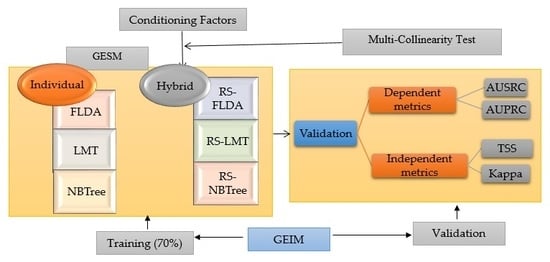
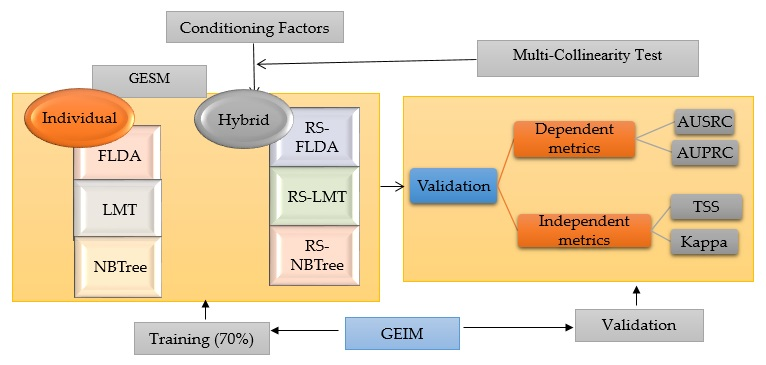
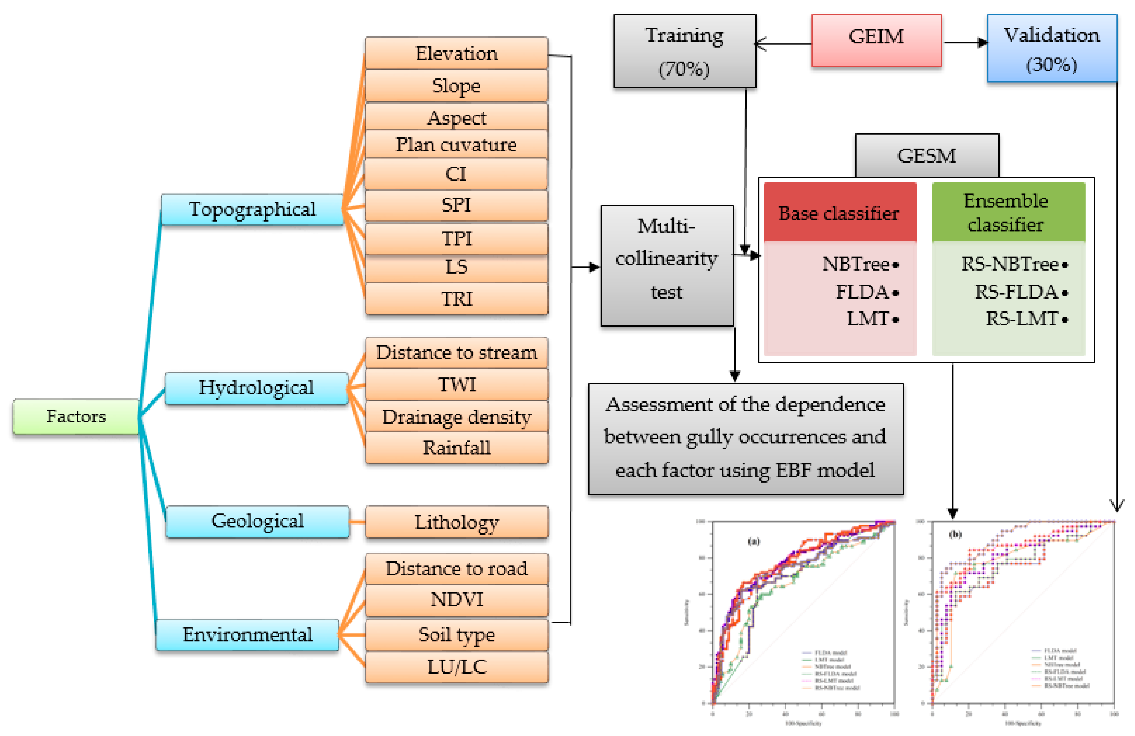
As shown in Figure 4, this research consisted of four steps: 1—collection of data and database construction, 2—multicollinearity test using VIF and TOL, 3—modeling of gully erosion and preparation of gully erosion susceptibility and 4—validation of results.
3. Results
Our methodological workflow is summarized in Figure 4. The procedures involved analyses in GIS and Weka. Several components are shown, which we reported on separately in the following sections.
3.1. Predisposing Factors’ Effects
Table 4 reports the outcome of the EBF analyses, and, specifically, the parameter Bel, which was adopted here to assess the relationship between gully occurrences and each factor. Since each factor was originally reclassified, a Bel value was assigned separately to each class rather than to the factor as a whole. The greater the Bel value, the stronger the effect of the given class on gully erosion occurrence. The primary contributors to gullies are factors associated with overland flows. This is particularly evident for distance to road (lower than 500 m), which is assigned the highest Bel value of 6.7; drainage density (greater than 1.7 km/km2) ranks second with a Bel value of 4.2; third is the stream power index (11.9 > SPI > 14.9) with a Bel value of 4.1 and fourth is the topographic wetness index (TWI > 12.0) with a Bel value of 4.0. These hydrological factors indicate a clear hydrological control on whether an area is prone to gully occurrence that far surpasses the effects of all other factor considered in this study. In fact, the four Bel values reported above far exceed the Bel values retrieved for the other factors, sometimes by one order of magnitude. This is an important finding that places the importance of hydrology above geomorphology and the other thematic properties in terms of contributing to gully erosion.
We could interpret the interconnected effects of the abovementioned factors in a simple schematic model in which the role of distance to road initially controls the total runoff over the road network. Roads are barriers to infiltration processes and promote runoff in their proximity, which in turn may be captured by the evidential belief function as a driver for gully erosion. The resulting runoff can travel to the surrounding drainage system, especially in cases where the drainage network is particularly dense (picked up by the drainage density). For those drainage branches where the morphology controls: 1) the energy of the overland flows (carried by the SPI), giving rise to potential turbulent hydrodynamics and 2) the water confluence and potential stagnation (TWI effect) through which gully erosional conditions are promoted.
An alternative interpretation to the above scheme is based on the assumption that the overland water coming from road-driven runoff accumulates in the neighboring streams. This can be assumed because of the high Bel value (2.2) assigned to distance to the stream (lower than 100 m). Taking aside the predominant role of hydrological properties, minor but still significantly influencing factors could be recognized in eastward facing aspect (Bel = 1.9), low to average rainfall discharges (66.3 < rain < 84.9, Bel = 1.6), low to medium greenness (0.043 < NDVI < 0.132), fluvial and piedmont conglomerates (Bel = 2.0), marshland cover type (kavir Bel = 1.7) and Entisols/Aridisols (Bel = 1.5).
Under consideration of these relevant factors’ subset, the previous interpretation scheme can be expanded to accommodate for specific morphometric exposition under relatively low precipitation regimes. Moreover, vegetation is scarce but not completely absent. A complete absence of vegetation usually corresponds to rock outcrops where erosion rates are extremely low because of the material properties of the rock. Conversely, areas with low to medium vegetation are often associated with the presence of soil that is not protected by leaves or stabilized by roots. Conglomerates are usually unconsolidated and unsorted sediments in the area, which can break down and be washed away. Furthermore, kavir and Aridisols, which are soluble deposits, are both indicative of regions where salt crusts frequently cover the landscape in Iran.
3.2. Susceptibility Mapping
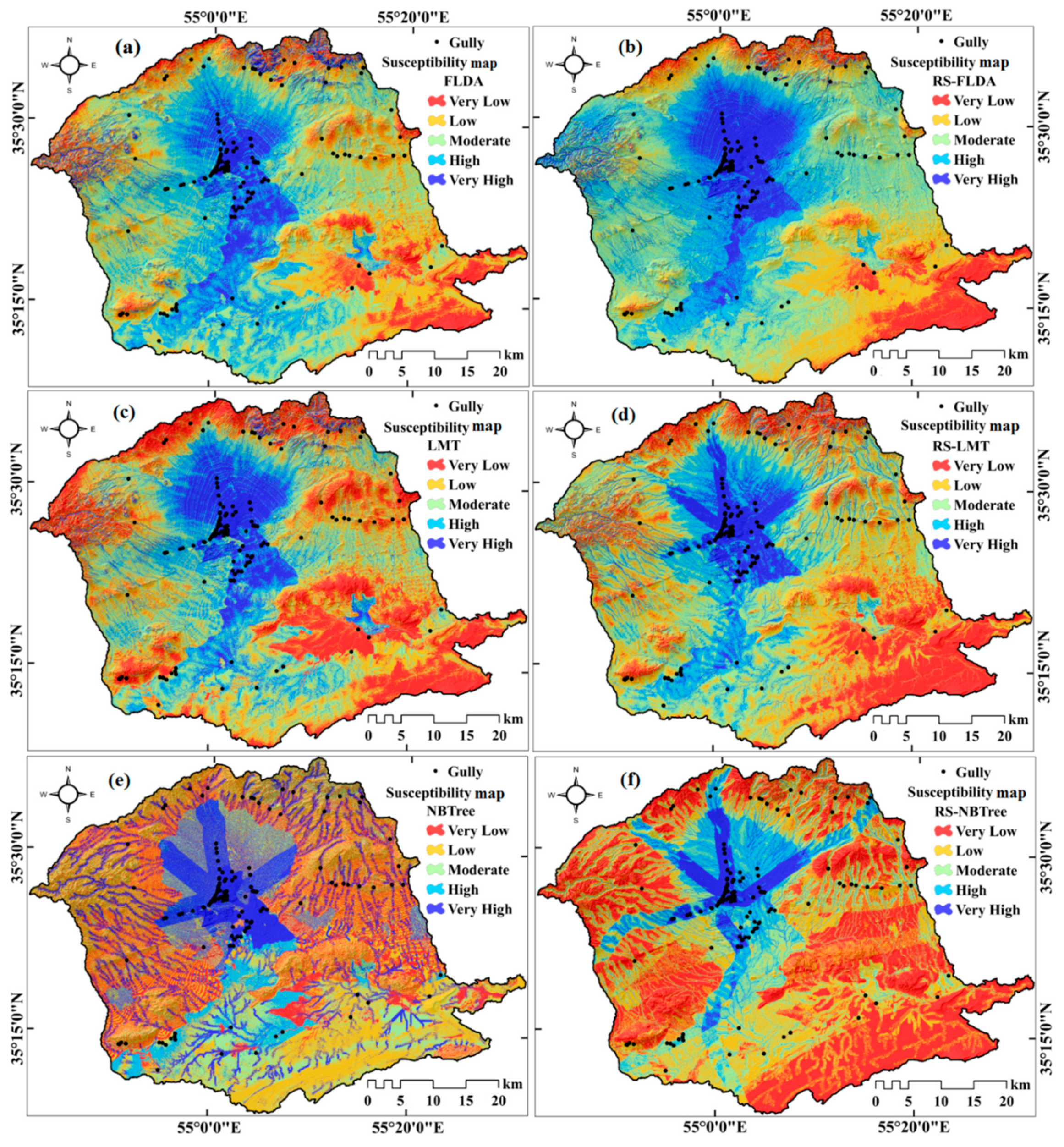
The application of FLDA, LMT and NBTree and the corresponding ensembles with RS meta classifier is summarized in Figure 5, where each susceptibility map is shown. The three basic models show significantly different patterns, especially the NBTree where the maps reproduce the patterns shown in the road network for the central region and the patterns shown in the distance to stream for the majority of the peripheral areas (see Figure 5).
The FLDA and the LMT produce smoother susceptibility estimates although the LMT is much stricter in depicting high and low probability areas. These graphical indications can be used as diagnostic tools to describe how rigidly each classification is performed. Machine learning algorithms are widely known for their classification capacity, albeit some issues can arise when they are used for prediction because to reach such extreme classification performance, they lose some flexibility over unknown instances. However, this appeared not to be the case in this work, for the actual prediction performed better than the model built with the training set (as will be discussed in the next section).
What stands out the most in observing the ensemble-driven susceptibility maps is that the models behaved very differently when combined with the Random SubSpace. The RS-FLDA was essentially unchanged with respect to the original FLDA. The RS-LMT strongly smoothed the patterns shown in the initial LMT map, and the most interesting effects are shown in the RS-NBTree. In this case, the gully-prone patterns were further specialized towards susceptible conditions. By specialized, we referred to the original smooth trend towards gully erosion conditions, which became much more confined to a narrow range of high susceptibility. This is particularly evident in the RS-NBTree map, where the very highly susceptible zones corresponding to the road corridors shown in the NBTree map became even narrower in the RS-NBTree. This implies that the ensemble procedure improved the ability of the simpler models to recognize gully-prone conditions. We numerically translate this “narrowing” effect in Table 5, where the NBTree is shown to have its very high susceptibility class shrunk when combined with the Random SubSpace. In Table 5, the behavior described based on the susceptibility maps for the FLDA and LMT (plus ensemble) are also numerically confirmed. The former class frequencies do not change substantially from FLDA to RS-FLDA, and the LMT became more normally distributed in the RS-LMT.
3.3. Model Performance
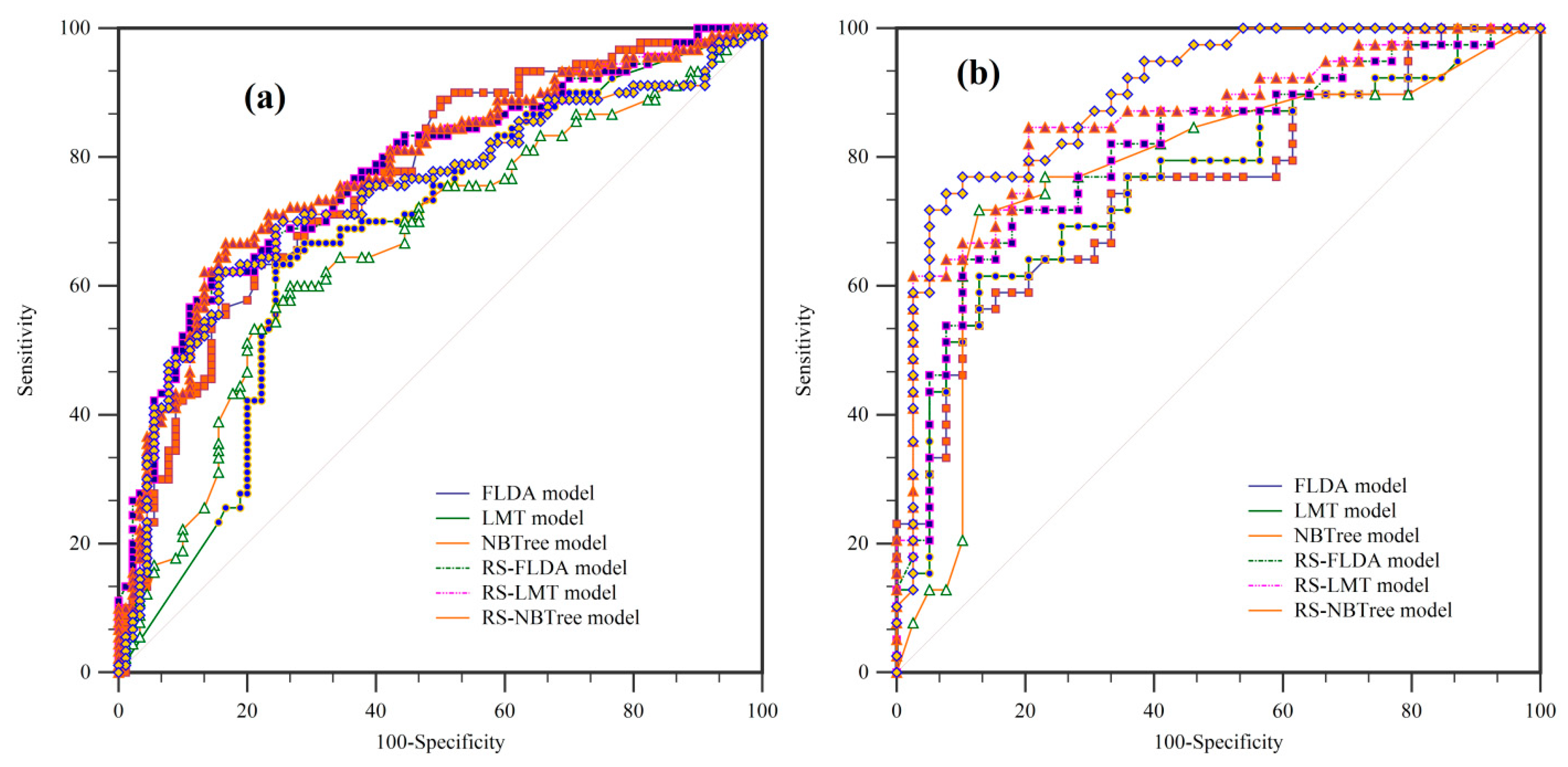
We initially assessed each model using ROC curves. Figure 6 summarizes the ROCs for each of the six models, both for the calibration (panel a) and validation (panel b) subsets. We recall here that the greater sparsity in the validation ROCs was due to the smaller number of data points. However, even though the calibration model is trained to describe gully-prone conditions solely based on the corresponding subset, the validation performances were even better (see Table 6). This must be a data specific feature because, generally, any training model outperformed the testing one. However, such behavior suggests that the gully-prone conditions in the area are quite consistent. In addition to the considerations above, we further examined both the changes between the simple and ensemble models as well as considering additional performance metrics. In fact, the ensemble models consistently outperformed the single ones, with the overall best being the validation RS-NBTree (AUC = 0.898) set. This is an interesting case where the calibration and validation performances are ranked differently among the ensemble models. In fact, the RS-NBTree is the worst model when tested with the training subset. This behavior may indicate a greater flexibility of the RS-NBTree compared to the other two models. In terms of auxiliary metrics, we also reported the Kappa and the TSS in Table 6. There, the relative ranks and the overall classification of model performance remain unchanged. The K suggests a substantial agreement across all models with a clear spike close to perfect prediction uniquely associated with RS-NBTree (K = 0.75). Furthermore, albeit a clear classification for the TSS has not been defined, several studies define high performances as anything above the 0.5 threshold (see [59]). Therefore, similar considerations to the one made for the AUC can be confirmed even from cutoff-dependent metrics.
4. Discussion and Conclusions
4.1. General Overview and Novelty
In the last decade, ensemble models have increasingly been applied in various scientific fields, which indicates their usefulness in improving predictive performance and reducing overfit with respect to single classifiers [9,74].
The novel idea behind the ensemble model is that any model is affected by two main sources of bias. The first one is inherent to the data one uses. For instance, incomplete inventories can heavily bias a model. Let us assume that we only had mapped gullies in proximity to the road network, the use of this biased dataset would have led to different associations with respect to the predisposing factors and hence, would have produced a different susceptibility pattern. Therefore, the best way to tackle this issue is either to use the best possible data and assume it to be an appropriate representation of reality, or to disregard the use of predisposing factors that are sensitive to the bias (in this theoretical example the distance to road should be removed). The second source of bias is caused by the method one adopts to model the gully erosion susceptibility. In fact, no matter how simple or complex a model may be, it performs in a way that is unique to the method itself. Therefore, from a wider perspective, each method, to some extent, leads to a different data treatment and susceptibility result. One way to cope with this methodological bias is to create a multi-model or ensemble model environment. In fact, the combination of more than one model helps to generalize the predictive results. A better generalization in the context of prediction can lead any given model to adapt to the new validation dataset, therefore reducing overfitting issues at the calibration stage and increasing performance during the validation one.
In this work, our results confirm both strengths of such a method. The dataset used for the analyses was repeatedly fed to each algorithm. Hence, changes in performance are unique due to the difference in the way the data is modeled.
4.2. Methodological Considerations
Our ensemble models consistently outperformed the corresponding simple models. Of the ensembles, the RS-NBTree performed significantly better than the other two. This is an important indicator and confirmation of how merging different results can improve the model flexibility. However, it is also important to note how each of the models we tested proved to be flexible enough without the intervention of the Random SubSpace with respect to the training and validation set. In fact, the Fisher’s linear discriminant function did not show any performance variation between training and testing in all metrics we explored. In any other case, this would already be an achievement but, furthermore, the other two methods we tested showed an improvement when predicting the unknown gully erosion dataset using the FLDA model. Conversely, the LMT and NBTree both demonstrated a greater adaptability, being able to explain the validation set even better than the calibration. However, of the two methods, the NBTree performed better, especially when combined with the Random SubSpace [75].
An NBTree is a combination of the decision tree (DT) and naïve Bayes (NB) algorithms, which are effective classifiers for classification problems [76]. However, the performance of an NBTree depends on the independence assumption [77]. Accordingly, ensemble (meta) classifiers such as the RS technique could improve the performance of single (weak) classifiers and enhance the results of the goodness-of-fit and prediction accuracies [77].
The RS meta classifier has already been reported to be a strong tool to build a reliable ensemble model, even compared to other ensembles [78]. In our case, the results we obtained are well in line with other studies, such as Shirzadi et al. [76], Pham et al. [79], Jebur et al. [80], Bui et al. [81], Bui et al. [82], Chen et al. [83], Pham et al. [84] and Hong et al. [85], where the ability of these meta-classifier and ensemble classifier models to reduce overfit and improve the accuracy has already been highlighted.
4.3. Applicability
Our results showed that the models’ performance could contribute valuable information for local planners. Since the arid to semi-arid environment in Iran can change quite rapidly from one catchment to another, be it in terms of temperatures or precipitation regimes, or simply in the landscape arrangement, it is especially important to have accurate and robust models to support decision making [31]. Therefore, greater model flexibility can support the choice of one method over another. We extended the usual performance assessment (area under the ROC curve) to include additional metrics (Cohen’s Kappa and True Skill Statistics), more versed in summarizing the classification of positives and negatives. Nevertheless, the three metrics reached a similar conclusion. Therefore, although we cannot generalize, for the present case it appears that the AUC alone would have been enough, which also justifies its adoption over any other metrics in the literature [74].
4.4. Interpretability
Concerning the association between gully erosion occurrences and causative factors, the patterns highlighted by the EBF appeared to be realistic and geomorphologically sound [9]. The primary contributors to gullying corresponded to hydrological or hydrologically related parameters. A clear conceptual scheme could even be drawn where the distance to road drives the initial runoff into the neighboring drainage and landscape incisions (distance to stream) where the combined action of the erosive power of running water (stream power index) and the tendency to drive and retain that water in a given location (topographic wetness index) set the conditions for gully erosion under climatic stress (rainfall). Ultimately, the conceptual scheme is completed by including eastward facing regions where a conglomeratic bedrock upwardly transitions to soluble soils rich in salt crusts exposed by weathering due to lack of vegetation protection.
Being able to draw such detailed conceptual schemes is the core of any study where causative relations between factors and gullies are explored. In fact, susceptibility maps can point out regions where actions should be taken to reduce or prevent gully erosion. However, the decision on what actual properties of the system should be addressed comes from understanding those that play a major role.
4.5. Summary and Relevance in Arid to Semi-arid Environments
The Iranian scientific community has recently focused on soil erosion. More specifically, they focused on gully erosion processes in Iran with the main goal of creating susceptibility models at the catchment scale. Our work aligns with this broader theme by testing three machine learning tools (FLDA, LMT and NBTree) and their “ensembled” extensions combined with RS, leaving the factors’ influence interpretation to EBF. The NBTree-RS showed flexibility far greater than that of the other methods tested in this work, and even compared to other published results. This is an important finding because a model able to adapt and predict an unknown dataset can support transferability studies. This type of application essentially builds models in a given region where data is relatively rich and predicts gully-prone conditions in regions where data is lacking, either because of missing processes or missing inventory maps. At the same time, EBF provided a clear picture of which factors are promoting gullying within the study area. This is an additional strength of EBF because implementing remediation practices relies on prioritizing investments over specific tasks. For instance, in this work, hydrological properties influence gullies to a greater extent than the other factors do. Therefore, investments can be made to control overland water fluxes. Overall, this work originated out of an Iranian scientific need, but its applicability and considerations are much more general. For instance, ensemble models do make a difference. The general perspective interprets the strength of ensemble models to be two-fold. The first states that “assembling” several models into one can smooth out specific biases resulting from the algorithmic structure. The second highlights “assembling” to be an efficient way to make a single model able to deal with large variations in the data, especially for prediction. In this study, we confirmed the second statement, for every single model we tested was significantly improved when combined with the RS meta classifier. Specifically, the performance of the NBTree-RS model supports its use in other geographic contexts, also for transferability purposes.
Author Contributions
Methodology, A.A.; formal analysis, A.A., W.C.; investigation, A.A., T.B., and D.T.B.; writing—original draft preparation, A.A., L.L.; writing—review and editing, A.A., L.L., D.T.B., and T.B. All authors have read and agreed to the published version of the manuscript.
Funding
This research was partly funded by the Austrian Science Fund (FWF) through the Doctoral College GIScience (DK W 1237-N23) at the University of Salzburg.
Conflicts of Interest
The authors declare no conflict of interest.
References
- Dube, F.; Nhapi, I.; Murwira, A.; Gumindoga, W.; Goldin, J.; Mashauri, D.A. Potential of weight of evidence modelling for gully erosion hazard assessment in Mbire District—Zimbabwe. Phys. Chem. Earth 2014, 67, 145–152. [Google Scholar] [CrossRef]
- Tomlinson, R.F. Thinking About GIS: Geographic Information System Planning for Managers, 1st ed.; ESRI, Inc.: Redlands, CA, USA, 2007. [Google Scholar]
- Conoscenti, C.; Angileri, S.; Cappadonia, C.; Rotigliano, E.; Agnesi, V.; Märker, M. Gully erosion susceptibility assessment by means of GIS-based logistic regression: A case of Sicily (Italy). Geomorphology 2014, 204, 399–411. [Google Scholar] [CrossRef] [Green Version]
- Rhoads, B.L. Statistical models of fluvial systems. Geomorphology 1992, 5, 433–455. [Google Scholar] [CrossRef]
- Lee, S.; Pradhan, B. Landslide hazard mapping at Selangor, Malaysia using frequency ratio and logistic regression models. Landslides 2007, 4, 33–41. [Google Scholar] [CrossRef]
- Rahmati, O.; Haghizadeh, A.; Pourghasemi, H.R.; Noormohamadi, F. Gully erosion susceptibility mapping: The role of GIS-based bivariate statistical models and their comparison. Nat. Hazards 2016, 82, 1231–1258. [Google Scholar] [CrossRef]
- Süzen, M.L.; Doyuran, V. A comparison of the GIS based landslide susceptibility assessment methods: Multivariate versus bivariate. Environ. Geol. 2004, 45, 665–679. [Google Scholar] [CrossRef]
- Süzen, M.L.; Doyuran, V. Data driven bivariate landslide susceptibility assessment using geographical information systems: A method and application to Asarsuyu catchment, Turkey. Eng. Geol. 2004, 71, 303–321. [Google Scholar] [CrossRef]
- Arabameri, A.; Pradhan, B.; Rezaei, K.; Yamani, M.; Pourghasemi, H.R.; Lombardo, L. Spatial modelling of gully erosion using evidential belief function, logistic regression, and a new ensemble of evidential belief function–logistic regression algorithm. Land Degrad. Dev. 2018, 29, 4035–4049. [Google Scholar] [CrossRef]
- Lombardo, L.; Mai, P.M. Presenting logistic regression-based landslide susceptibility results. Eng. Geol. 2018, 244, 14–24. [Google Scholar] [CrossRef]
- Lombardo, L.; Cama, M.; Maerker, M.; Rotigliano, E. A test of transferability for landslides susceptibility models under extreme climatic events: Application to the Messina 2009 disaster. Nat. Hazards 2014, 74, 1951–1989. [Google Scholar] [CrossRef]
- Castro Camilo, D.; Lombardo, L.; Mai, P.M.; Dou, J.; Huser, R. Handling high predictor dimensionality in slope-unit-based landslide susceptibility models through LASSO-penalized Generalized Linear Model. Environ. Model. Softw. 2017, 97, 145–156. [Google Scholar] [CrossRef] [Green Version]
- Beguería, S. Validation and evaluation of predictive models in hazard assessment and risk management. Nat. Hazards 2006, 37, 315–329. [Google Scholar] [CrossRef] [Green Version]
- Goetz, J.N.; Guthrie, R.H.; Brenning, A. Integrating physical and empirical landslide susceptibility models using generalized additive models. Geomorphology 2011, 129, 376–386. [Google Scholar] [CrossRef]
- Lombardo, L.; Opitz, T.; Huser, R. Point process-based modeling of multiple debris flow landslides using INLA: An application to the 2009 Messina disaster. Stoch. Environ. Res. Risk Assess. 2018, 2, 2179–2198. [Google Scholar] [CrossRef] [Green Version]
- Pourghasemi, H.R.; Rossi, M. Landslide susceptibility modeling in a landslide prone area in Mazandarn Province, north of Iran: A comparison between GLM, GAM, MARS, and M-AHP methods. Theor. Appl. Climatol. 2017, 130, 609–633. [Google Scholar] [CrossRef]
- Felicísimo, Á.M.; Cuartero, A.; Remondo, J.; Quirós, E. Mapping landslide susceptibility with logistic regression, multiple adaptive regression splines, classification and regression trees, and maximum entropy methods: A comparative study. Landslides 2013, 10, 175–189. [Google Scholar] [CrossRef]
- Tien Bui, D.; Pradhan, B.; Lofman, O.; Revhaug, I. Landslide susceptibility assessment in vietnam using support vector machines, decision tree, and Naïve Bayes Models. Math. Prob. Eng. 2012, 2012, 1–26. [Google Scholar] [CrossRef] [Green Version]
- Lombardo, L.; Fubelli, G.; Amato, G.; Bonasera, M. Presence-only approach to assess landslide triggering-thickness susceptibility: A test for the Mili catchment (north-eastern Sicily, Italy). Nat. Hazards 2016, 84, 565–588. [Google Scholar] [CrossRef]
- Lee, M.J.; Choi, J.W.; Oh, H.J.; Won, J.S.; Park, I.; Lee, S. Ensemble-based landslide susceptibility maps in Jinbu area, Korea. In Terrigenous mass movements. Environ. Earth Sci. 2012, 1, 23–37. [Google Scholar] [CrossRef]
- Althuwaynee, O.F.; Pradhan, B.; Park, H.J.; Lee, J.H. A novel ensemble bivariate statistical evidential belief function with knowledge-based analytical hierarchy process and multivariate statistical logistic regression for landslide susceptibility mapping. Catena 2014, 114, 21–36. [Google Scholar] [CrossRef]
- Pourghasemi, H.R.; Kerle, N. Random forests and evidential belief function-based landslide susceptibility assessment in Western Mazandaran Province, Iran. Environ. Earth Sci. 2016, 75, 185. [Google Scholar] [CrossRef]
- Zakerinejad, R.; Maerker, M. An integrated assessment of soil erosion dynamics with special emphasis on gully erosion in the Mazayjan basin, southwestern Iran. Nat. Hazards 2015, 79, 25–50. [Google Scholar] [CrossRef]
- Zabihi, M.; Mirchooli, F.; Motevalli, A.; Darvishan, A.K.; Pourghasemi, H.R.; Zakeri, M.A.; Sadighi, F. Spatial modelling of gully erosion in Mazandaran Province, northern Iran. Catena 2018, 161, 1–13. [Google Scholar] [CrossRef]
- Rahmati, O.; Tahmasebipour, N.; Haghizadeh, A.; Pourghasemi, H.R.; Feizizadeh, B. Evaluating the influence of geo-environmental factors on gully erosion in a semi-arid region of Iran: An integrated framework. Sci. Total Environ. 2017, 579, 913–927. [Google Scholar] [CrossRef]
- Jafari, R.; Bakhshandehmehr, L. Quantitative mapping and assessment of environmentally sensitive areas to desertification in central Iran. Land Degrad. Dev. 2016, 7, 108–119. [Google Scholar] [CrossRef]
- IRIMO. Summary Reports of Iran’s Extreme Climatic Events. Ministry of Roads and Urban Development, Iran Meteorological Organization. Available online: www.cri.ac.ir (accessed on 12 August 2018).
- GSI. Geology Survey of Iran. Available online: http://www.gsi.ir/Main/Lang_en/index.html (accessed on 12 August 2018).
- Arabameri, A.; Pradhan, B.; Rezaei, K.; Conoscenti, C. Gully erosion susceptibility mapping using GIS-based multi-criteria decision analysis techniques. CATENA 2019, 180, 282–297. [Google Scholar] [CrossRef]
- Arabameri, A.; Pradhan, B.; Rezaei, K. Gully erosion zonation mapping using integrated geographically weighted regression with certainty factor and random forest models in GIS. J. Environ. Manag. 2019, 232, 928–942. [Google Scholar] [CrossRef]
- Arabameri, A.; Pradhan, B.; Rezaei, K. Spatial prediction of gully erosion using ALOS PALSAR data and ensemble bivariate and data mining models. Geosci. J. 2019, 1–18. [Google Scholar] [CrossRef]
- Arabameri, A.; Pradhan, B.; Rezaei, K.; Lee, C.-W. Assessment of Landslide Susceptibility Using Statistical-and Artificial Intelligence-based FR–RF Integrated Model and Multiresolution DEMs. Remote Sens. 2019, 11, 999. [Google Scholar] [CrossRef] [Green Version]
- Arabameri, A.; Pradhan, B.; Rezaei, K.; Sohrabi, M.; Kalantari, Z. GIS-based landslide susceptibility mapping using numerical risk factor bivariate model and its ensemble with linear multivariate regression and boosted regression tree algorithms. J. Mt. Sci. 2019, 16, 595–618. [Google Scholar] [CrossRef]
- Arabameri, A.; Rezaei, K.; Cerdà, A.; Conoscenti, C.; Kalantari, Z. A comparison of statistical methods and multi-criteria decision making to map flood hazard susceptibility in Northern Iran. Sci. Total Environ. 2019, 660, 443–458. [Google Scholar] [CrossRef] [PubMed]
- Dempster, A.P. Upper and lower probabilities induced by a multi valued mapping. Ann. Math. Stat. 1967, 38, 325–339. [Google Scholar] [CrossRef]
- Shafer, G. A Mathematical Theory of Evidence; Princeton University Press: Priceton, NJ, USA, 1976. [Google Scholar]
- Bal, H.; Örkcü, H. Data Envelopment Analysis Approach to Two-group Classification Problems and an Experimental Comparison with Some Classification Models. Hacet. J. Math. Stat. 2007, 36, 169–180. [Google Scholar]
- Zhao, X.; Chen, W. Gis-based evaluation of landslide susceptibility models using certainty factors and functional trees-based ensemble techniques. Appl. Sci. 2020, 10, 16. [Google Scholar] [CrossRef] [Green Version]
- Ramos-Cañón, A.M.; Prada-Sarmiento, L.F.; Trujillo-Vela, M.G.; Macías, J.P.; Santos-R, A.C. Linear discriminant analysis to describe the relationship between rainfall and landslides in Bogotá, Colombia. Landslides 2016, 13, 671–681. [Google Scholar] [CrossRef]
- Durrant, R.J.; Kaban, A. Compressed fisher linear discriminant analysis: Classification of randomly projected data. In Proceedings of the 16th ACM SIGKDD International Conference on Knowledge Discovery and Data Mining, Washington, DC, USA, 25–28 July 2010; pp. 1119–1128. [Google Scholar]
- Landwehr, N.; Hall, M.; Frank, E. Logistic Model Trees. Mach. Learn. 2005, 59, 161–205. [Google Scholar] [CrossRef] [Green Version]
- Chen, W.; Xie, X.; Wang, J.; Pradhan, B.; Hong, H.; Tien Bui, D.; Duan, Z.; Ma, J. A comparative study of logistic model tree, random forest, and classification and regression tree models for spatial prediction of landslide susceptibility. CATENA 2017, 151, 147–160. [Google Scholar] [CrossRef] [Green Version]
- Tien Bui, D.; Tuan, T.A.; Klempe, H.; Pradhan, B.; Revhaug, I. Spatial prediction models for shallow landslide hazards: A comparative assessment of the efficacy of support vector machines, artificial neural networks, kernel logistic regression, and logistic model tree. Landslides 2016, 13, 361–378. [Google Scholar] [CrossRef]
- Zhang, G.; Fang, B. LogitBoost classifier for discriminating thermophilic and mesophilic proteins. J. Biotechnol. 2007, 127, 417–424. [Google Scholar] [CrossRef]
- Wang, K. Network data management model based on Naïve Bayes classifier and deep neural networks in heterogeneous wireless networks. Comput. Electr. Eng. 2019, 75, 135–145. [Google Scholar] [CrossRef]
- He, Q.; Shahabi, H.; Shirzadi, A.; Li, S.; Chen, W.; Wang, N.; Chai, H.; Bian, H.; Ma, J.; Chen, W.; et al. Landslide spatial modelling using novel bivariate statistical based Naïve Bayes, RBF Classifier, and RBF Network machine learning algorithms. Sci. Total Environ. 2019, 663, 1–15. [Google Scholar] [CrossRef] [PubMed]
- Chen, W.; Xie, X.; Peng, J.; Wang, J.; Duan, Z.; Hong, H. GIS-based landslide susceptibility modelling: A comparative assessment of kernel logistic regression, Naïve-Bayes tree, and alternating decision tree models. Geomat. Nat. Hazards Risk 2017, 8, 950–973. [Google Scholar] [CrossRef] [Green Version]
- Barandiaran, I. The random subSpace method for constructing decision forests. IEEE 1998, 20, 832–844. [Google Scholar]
- Rokach, L.; Maimon, O.Z. Data Mining with Decision Trees: Theory and Applications, 2nd ed.; World scientific: Singapore, 2008. [Google Scholar]
- Lewis, R.J. An introduction to classification and regression tree (CART) analysis. In Proceedings of the Annual Meeting of the Society for Academic Emergency Medicine, San Francisco, CA, USA, 22–25 May 2000; Volume 14. [Google Scholar]
- Gey, S.; Nedelec, E. Model Selection for CART Regression Trees; IEEE: Piscataway, NJ, USA, 2005; Volume 51, pp. 658–670. [Google Scholar]
- Gashler, M.; Giraud-Carrier, C.; Martinez, T. Decision tree ensemble: Small heterogeneous is better than large homogeneous. In Proceedings of the 2008 Seventh International Conference on Machine Learning and Applications, San Francisco, CA, USA, 11–13 December 2008; pp. 900–905. [Google Scholar]
- Arabameri, A.; Rezaei, K.; Cerda, A.; Lombardo, L.; Rodrigo-Comino, J. GIS-based groundwater potential mapping in Shahroud plain, Iran. A comparison among statistical (bivariate and multivariate), data mining and MCDM approaches. Sci. Total Environ. 2019, 658, 160–177. [Google Scholar] [CrossRef]
- Arabameri, A.; Pradhan, B.; Rezaei, K.; Saro, L.; Sohrabi, M. An ensemble model for landslide susceptibility mapping in a forested area. Geochem. Int. 2019, 1–18. [Google Scholar] [CrossRef]
- Steger, S.; Brenning, A.; Bell, R.; Glade, T. The propagation of inventory-based positional errors into statistical landslide susceptibility models. Nat. Hazards Earth Syst. Sci. 2016, 16, 2729–2745. [Google Scholar] [CrossRef] [Green Version]
- Chen, W.; Pourghasemi, H.R.; Naghibi, S.A. Prioritization of landslide conditioning factors and its spatial modeling in shangnan county, china using gis-based data mining algorithms. Bull. Eng. Geol. Environ. 2018, 77, 611–629. [Google Scholar] [CrossRef]
- Chen, W.; Panahi, M.; Khosravi, K.; Pourghasemi, H.R.; Rezaie, F.; Parvinnezhad, D. Spatial prediction of groundwater potentiality using anfis ensembled with teaching-learning-based and biogeography-based optimization. J. Hydrol. 2019, 572, 435–448. [Google Scholar] [CrossRef]
- Chen, W.; Tsangaratos, P.; Ilia, I.; Duan, Z.; Chen, X. Groundwater spring potential mapping using population-based evolutionary algorithms and data mining methods. Sci. Total Environ. 2019, 684, 31–49. [Google Scholar] [CrossRef]
- Chen, W.; Li, Y.; Xue, W.; Shahabi, H.; Li, S.; Hong, H.; Wang, X.; Bian, H.; Zhang, S.; Pradhan, B.; et al. Modeling flood susceptibility using data-driven approaches of naïve bayes tree, alternating decision tree, and random forest methods. Sci. Total Environ. 2020, 701, 134979. [Google Scholar] [CrossRef]
- Chen, W.; Hong, H.; Panahi, M.; Shahabi, H.; Wang, Y.; Shirzadi, A.; Pirasteh, S.; Alesheikh, A.A.; Khosravi, K.; Panahi, S.; et al. Spatial prediction of landslide susceptibility using gis-based data mining techniques of anfis with whale optimization algorithm (woa) and grey wolf optimizer (gwo). Appl. Sci. 2019, 9, 3755. [Google Scholar] [CrossRef] [Green Version]
- Arabameri, A.; Chen, W.; Blaschke, T.; Tiefenbacher, J.P.; Pradhan, B.; Tien Bui, D. Gully Head-Cut Distribution Modeling Using Machine Learning Methods—A Case Study of N.W. Iran. Water 2020, 12, 16. [Google Scholar] [CrossRef] [Green Version]
- Arabameri, A.; Pradhan, B.; Pourghasemi, H.; Rezaei, K.; Kerle, N. Spatial modelling of gully erosion using GIS and R programing: A comparison among three data mining algorithms. Appl. Sci. 2018, 8, 1369. [Google Scholar] [CrossRef] [Green Version]
- Arabameri, A.; Cerda, A.; Rodrigo-Comino, J.; Pradhan, B.; Sohrabi, M.; Blaschke, T.; Tien Bui, D. Proposing a Novel Predictive Technique for Gully Erosion Susceptibility Mapping in Arid and Semi-arid Regions (Iran). Remote Sens. 2019, 11, 2577. [Google Scholar] [CrossRef] [Green Version]
- Arabameri, A.; Cerda, A.; Tiefenbacher, J.P. Spatial Pattern Analysis and Prediction of Gully Erosion Using Novel Hybrid Model of Entropy-Weight of Evidence. Water 2019, 11, 1129. [Google Scholar] [CrossRef] [Green Version]
- Arabameri, A.; Roy, J.; Saha, S.; Blaschke, T.; Ghorbanzadeh, O.; Tien Bui, D. Application of Probabilistic and Machine Learning Models for Groundwater Potentiality Mapping in Damghan Sedimentary Plain, Iran. Remote Sens. 2019, 11, 3015. [Google Scholar] [CrossRef] [Green Version]
- Roy, J.; Saha, S.; Arabameri, A.; Blaschke, T.; Bui, D.T. A Novel Ensemble Approach for Landslide Susceptibility Mapping (LSM) in Darjeeling and Kalimpong Districts, West Bengal, India. Remote Sens. 2019, 11, 2866. [Google Scholar] [CrossRef] [Green Version]
- Arabameri, A.; Chen, W.; Loche, M.; Zhao, X.; Li, Y.; Lombardo, L.; Cerda, A.; Pradhan, B.; Bui, D.T. Comparison of machine learning models for gully erosion susceptibility mapping. Geosci. Front. 2019, in press. [Google Scholar] [CrossRef]
- Lombardo, L.; Cama, M.; Conoscenti, C.; Märker, M.; Rotigliano, E. Binary logistic regression versus stochastic gradient boosted decision trees in assessing landslide susceptibility for multiple-occurring landslide events: Application to the 2009 storm event in Messina (Sicily, southern Italy). Nat. Hazards 2015, 79, 1621–1648. [Google Scholar] [CrossRef]
- Rahmati, O.; Kornejady, A.; Samadi, M.; Deo, R.C.; Conoscenti, C.; Lombardo, L.; Dayal, K.; Taghizadeh-Mehrjardi, R.; Pourghasemi, H.R.; Kumar, S.; et al. PMT: New analytical framework for automated evaluation of geo-environmental modelling approaches. Sci. Total Environ. 2019, 664, 296–311. [Google Scholar] [CrossRef]
- Frattini, P.; Crosta, G.; Carrara, A. Techniques for evaluating the performance of landslide susceptibility models. Eng. Geol. 2010, 111, 62–72. [Google Scholar] [CrossRef]
- Allouche, O.; Tsoar, A.; Kadmon, R. Assessing the accuracy of species distribution models: Prevalence, kappa and the true skill statistic (TSS). J. Appl. Ecol. 2006, 43, 1223–1232. [Google Scholar] [CrossRef]
- McHugh, M.L. Interrater reliability: The kappa statistic. Biochem. Med. 2012, 22, 276–282. [Google Scholar] [CrossRef]
- Cohen, J. A coefficient of agreement for nominal scales. Educ. Psychol. Meas. 1960, 20, 37–46. [Google Scholar] [CrossRef]
- Chen, W.; Li, H.; Hou, E.; Wang, S.; Wang, G.; Panahi, M.; Li, T.; Peng, T.; Guo, C.; Niu, C.; et al. GIS-based groundwater potential analysis using novel ensemble weights-of-evidence with logistic regression and functional tree models. Sci. Total Environ. 2018, 634, 853–867. [Google Scholar] [CrossRef] [PubMed] [Green Version]
- Chen, W.; Hong, H.; Li, S.; Shahabi, H.; Wang, Y.; Wang, X.; Ahmad, B.B. Flood susceptibility modelling using novel hybrid approach of reduced-error pruning trees with bagging and random subSpace ensembles. J. Hydrol. 2019, 575, 864–873. [Google Scholar] [CrossRef]
- Shirzadi, A.; Bui, D.T.; Pham, B.T.; Solaimani, K.; Chapi, K.; Kavian, A.; Shahabi, H.; Revhaug, I. Shallow landslide susceptibility assessment using a novel hybrid intelligence approach. Environ. Earth Sci. 2017, 76, 60. [Google Scholar] [CrossRef]
- Pham, B.T.; Bui, D.T.; Prakash, I.; Dholakia, M. Rotation forest fuzzy rule-based classifier ensemble for spatial prediction of landslides using GIS. Nat. Hazards 2016, 83, 97–127. [Google Scholar] [CrossRef]
- Pham, T.B.; Shirzadi, A.; Shahabi, H.; Omidvar, E.; Singh, S.K.; Sahana, M.; Talebpour Asl, D.; Bin Ahmad, B.; Kim Quoc, N.; Lee, S. Landslide Susceptibility Assessment by Novel Hybrid Machine Learning Algorithms. Sustainability 2019, 11, 4386. [Google Scholar] [CrossRef] [Green Version]
- Pham, B.T.; Bui, D.T.; Pham, H.V.; Le, H.Q.; Prakash, I.; Dholakia, M. Landslide hazard assessment using random subspace fuzzy rules based classifier ensemble and probability analysis of rainfall data: A case study at Mu Cang Chai district, Yen Bai province (Vietnam). J. Indian Soc. Remote Sens. 2017, 45, 673–683. [Google Scholar] [CrossRef]
- Jebur, M.N.; Pradhan, B.; Tehrany, M.S. Optimization of landslide conditioning factors using very high-resolution airborne laser scanning (lidar) data at catchment scale. Remote Sens. Environ. 2014, 152, 150–165. [Google Scholar] [CrossRef]
- Bui, D.T.; Pradhan, B.; Revhaug, I.; Tran, C.T. A comparative assessment between the application of fuzzy unordered rules induction algorithm and j48 decision tree models in spatial prediction of shallow landslides at lang son city, vietnam. In Remote Sensing Applications in Environmental Research; Springer: Berlin/Heidelberg, Germany, 2014; pp. 87–111. [Google Scholar]
- Bui, T.D.; Shirzadi, A.; Shahabi, H.; Chapi, K.; Omidavr, E.; Pham, B.T.; Talebpour Asl, D.; Khaledian, H.; Pradhan, B.; Panahi, M. A Novel Ensemble Artificial Intelligence Approach for Gully Erosion Mapping in a Semi-Arid Watershed (Iran). Sensors 2019, 19, 2444. [Google Scholar]
- Chen, W.; Shahabi, H.; Zhang, S.; Khosravi, K.; Shirzadi, A.; Chapi, K.; Pham, B.; Zhang, T.; Zhang, L.; Chai, H. Landslide susceptibility modeling based on gis and novel bagging-based kernel logistic regression. Appl. Sci. 2018, 8, 2540. [Google Scholar] [CrossRef] [Green Version]
- Pham, B.T.; Bui, D.T.; Prakash, I.; Dholakia, M. Hybrid integration of multilayer perceptron neural networks and machine learning ensembles for landslide susceptibility assessment at himalayan area (India) using GIS. Catena 2017, 149, 52–63. [Google Scholar] [CrossRef]
- Hong, H.; Liu, J.; Bui, D.T.; Pradhan, B.; Acharya, T.D.; Pham, B.T.; Zhu, A.-X.; Chen, W.; Ahmad, B.B. Landslide susceptibility mapping using j48 decision tree with adaboost, bagging and rotation forest ensembles in the guangchang area (China). Catena 2018, 163, 399–413. [Google Scholar] [CrossRef]
Figure 1.
Study area. (a) Location of Iran in the world, (b) location of study area in Iran and (c) location of training and validation gullies in the study area.
Figure 1.
Study area. (a) Location of Iran in the world, (b) location of study area in Iran and (c) location of training and validation gullies in the study area.

Figure 2.
Sample of mapped gullies in the study area.

Figure 3.
Gully erosion conditioning factors. (a) elevation, (b) slope, (c) aspect, (d) plan curvature, (e) convergence index (CI), (f) slope length (LS), (g) stream power index (SPI), (h) topography position index (TPI), (i) terrain ruggedness index (TRI), (j) topographical wetness index (TWI), (k) distance to stream, (l) drainage density, (m) rainfall, (n) distance to road, (o) NDVI (normalized difference vegetation index), (p) lithology, (q) land use/cover (LU/LC) and (r) soil type.


Figure 4.
Research flowchart of the present study.

Figure 5.
Gully erosion susceptibility mapping using different models (a–f).

Figure 6.
Validation of results. (a) Success rate curve and (b) prediction rate curve.


Table 1.
List of Predisposing Factors and their Source.
| ID | Predisposing Factor | Reference |
|---|---|---|
| 1 | Elevation | -- |
| 2 | Slope | Zevenbergen and Thorne, 1987 |
| 3 | Aspect | Zevenbergen and Thorne, 1987 |
| 4 | Planar Curvature | Heerdegen and Beran, 1982 |
| 5 | Convergence Index | Olaya and Conrad, 2009 |
| 6 | Topographic Wetness Index (TWI) | Beven and Kirkby, 1979 |
| 7 | Stream Power Index (SPI) | Moore et al., 1991 |
| 8 | Slope Length Factor (LS) | Desmet and Govers, 1996 |
| 9 | Terrain Ruggedness Index | Riley et al., 1999 |
| 10 | Topographic position Index | De Reu et al., 2013 |
| 11 | Drainage Density | -- |
| 12 | Distance to Stream | -- |
| 13 | Rainfall | -- |
| 14 | Distance to Road | -- |
| 15 | Normalized Difference Vegetation Index (NDVI) | -- |
| 16 | Land Use/Cover | -- |
| 17 | Lithology | -- |
| 18 | Soil Type | -- |
Table 2.
Lithology of the Study Area.
| Code | Lithology Description |
|---|---|
| A | Marl, gypsiferous marl and limestone, dacitic to andesitic volcano sediment, well bedded green tuff and tuffaceous shale, dacitic to andesitic volcanic, dacitic to andesitic volcano breccia Andesitic volcanic breccia, sandstone, marl and limestone, granite, pale-red, polygenic conglomerate and sandstone |
| B | Phyllite, slate and meta-sandstone, Jurassic dacite to andesite lava flows |
| C | Cretaceous rocks in general |
| D | Light-red to brown marl and gypsiferous marl with sandstone intercalations, red marl, gypsiferous marl, sandstone and conglomerate |
| E | Fluvial conglomerate, piedmont conglomerate and sandstone. |
| F | Salt flat, high-level piedmont fan and valley terrace deposits, low-level piedmont fan and valley terrace deposits, salt lake |
Table 3.
Multicollinearity Analysis of Gully Erosion Conditioning Factors.
| Factors | Collinearity Statistics | Factors | Collinearity Statistics | ||
|---|---|---|---|---|---|
| Tolerance | VIF | Tolerance | VIF | ||
| Distance to road | 0.370 | 2.702 | Distance to Stream | 0.596 | 1.677 |
| Rainfall | 0.321 | 3.098 | Slope | 0.612 | 1.525 |
| Convergence index | 0.586 | 1.707 | Aspect | 0.948 | 1.055 |
| Plan curvature | 0.656 | 1.524 | NDVI | 0.658 | 1.520 |
| Terrain Ruggedness Index | 0.558 | 2.286 | Topography wetness index | 0.357 | 2.911 |
| Elevation | 0.438 | 2.545 | Slope length | 0.874 | 1.144 |
| Stream power index | 0.419 | 2.346 | Lithology | 0.749 | 1.335 |
| Drainage density | 0.362 | 2.766 | Topographic Position Index | 0.564 | 1.772 |
| Soil type | 0.431 | 2.318 | Land use/land cover | 0.621 | 1.611 |
Table 4.
Spatial Analysis of Gully Erosion Conditioning Factors and Gully Locations using the Evidential Belief Function (EBF) Model.
Table 4.
Spatial Analysis of Gully Erosion Conditioning Factors and Gully Locations using the Evidential Belief Function (EBF) Model.
| Factors | Classes | Pixels in Domain | Number of Gullies | Bel |
|---|---|---|---|---|
| Elevation (m) | <819 | 1373897 | 46 | 1.006 |
| 819–1000 | 567118 | 29 | 1.536 | |
| 1000–1206 | 450512 | 9 | 0.600 | |
| 1206–1500 | 237673 | 6 | 0.758 | |
| >1500 | 73829 | 0 | 0.000 | |
| Slope (°) | <5 | 2270219 | 81 | 1.072 |
| 5–10 | 234394 | 6 | 0.769 | |
| 10–15 | 84199 | 3 | 1.070 | |
| 15–20 | 43477 | 0 | 0.000 | |
| 20–30 | 46247 | 0 | 0.000 | |
| >30 | 24488 | 0 | 0.000 | |
| Aspect | F | 135222 | 4 | 0.888 |
| N | 203003 | 4 | 0.915 | |
| NE | 244887 | 10 | 1.226 | |
| E | 395661 | 25 | 1.898 | |
| SE | 496849 | 24 | 1.451 | |
| S | 473666 | 13 | 0.824 | |
| SW | 342248 | 6 | 0.527 | |
| W | 223850 | 3 | 0.402 | |
| NW | 187643 | 1 | 0.160 | |
| Plan curvature (100/m) | Concave | 894313 | 31 | 1.041 |
| Flat | 901103 | 40 | 1.333 | |
| Convex | 907612 | 19 | 0.629 | |
| Convergence index (100/m) | <–39.6 | 275709 | 14 | 1.523 |
| –39.6 to –12.9 | 586976 | 22 | 1.124 | |
| –12.9–10.5 | 919934 | 28 | 0.913 | |
| 10.5–38 | 624756 | 18 | 0.864 | |
| >38 | 292694 | 8 | 0.820 | |
| LS (m) | <20 | 1531797 | 63 | 1.235 |
| 20–57.5 | 230099 | 9 | 1.175 | |
| 57.5–92.1 | 396472 | 9 | 0.682 | |
| 92.1–128.2 | 339443 | 4 | 0.354 | |
| >128.2 | 204840 | 5 | 0.733 | |
| <8.2 | 1023818 | 32 | 0.939 | |
| SPI | 8.2–9.9 | 1017957 | 30 | 0.885 |
| 9.9–11.9 | 489089 | 9 | 0.553 | |
| 11.9–14.9 | 140449 | 19 | 4.063 | |
| >14.9 | 31709 | 0 | 0.000 | |
| <−8 | 42635 | 3 | 2.113 | |
| TPI | –8 to –1.8 | 371266 | 17 | 1.375 |
| –1.8–1.9 | 2122669 | 69 | 0.976 | |
| 1.9–9.6 | 138072 | 1 | 0.218 | |
| >9.6 | 28385 | 0 | 0.000 | |
| <1.4 | 2031200 | 73 | 1.079 | |
| TRI | 1.4–3.9 | 421180 | 12 | 0.856 |
| 3.9–7.8 | 159763 | 5 | 0.940 | |
| 7.8–13.5 | 69390 | 0 | 0.000 | |
| >13.5 | 21495 | 0 | 0.000 | |
| TWI | <6.25 | 1087667 | 24 | 0.663 |
| 6.25–8.57 | 1013529 | 30 | 0.889 | |
| 8.57–11.97 | 465805 | 18 | 1.161 | |
| >11.97 | 136023 | 18 | 3.975 | |
| Distance to stream (m) | <100 | 645017 | 48 | 2.235 |
| 100–200 | 486406 | 15 | 0.926 | |
| 200–300 | 435933 | 9 | 0.620 | |
| 300–400 | 297487 | 7 | 0.707 | |
| >400 | 838184 | 11 | 0.394 | |
| Drainage density (km/km2) | <0.89 | 670956 | 9 | 0.403 |
| 0.89–1.25 | 1133824 | 27 | 0.715 | |
| 1.25–1.73 | 696610 | 26 | 1.121 | |
| >1.73 | 201639 | 28 | 4.171 | |
| Rainfall (mm) | <66.3 | 615156 | 8 | 0.391 |
| 66.3–84.9 | 1046810 | 54 | 1.549 | |
| 84.9–111.5 | 904755 | 28 | 0.929 | |
| 111.5–149.9 | 86955 | 0 | 0.000 | |
| >149.9 | 49353 | 0 | 0.000 | |
| Distance to road (m) | <500 | 142666 | 32 | 6.738 |
| 500–1000 | 134376 | 8 | 1.788 | |
| 1000–1500 | 129321 | 1 | 0.232 | |
| 1500–2000 | 125196 | 4 | 0.960 | |
| >2000 | 2171485 | 45 | 0.622 | |
| NDVI | <0.043 | 1279439 | 29 | 0.679 |
| 0.043–0.132 | 1417082 | 61 | 1.290 | |
| >0.132 | 873 | 0 | 0.000 | |
| Lithology | A | 578105 | 11 | 0.571 |
| B | 27122 | 2 | 2.213 | |
| C | 34563 | 0 | 0.000 | |
| D | 439618 | 22 | 1.502 | |
| E | 193927 | 13 | 2.011 | |
| F | 1427087 | 42 | 0.883 | |
| Agriculture | 2353 | 0 | 0.000 | |
| LU/LC | Bareland | 20180 | 0 | 0.000 |
| Kavir | 806162 | 46 | 1.712 | |
| Poorrange | 1460908 | 37 | 0.760 | |
| Rock | 296104 | 5 | 0.507 | |
| Saltlake | 99897 | 2 | 0.601 | |
| Saltland | 13808 | 0 | 0.000 | |
| Wetland | 1010 | 0 | 0.000 | |
| Bad Lands (a) | 241417 | 3 | 0.373 | |
| Rock Outcrops/Entisols (b) | 495473 | 13 | 0.787 | |
| Soil type | Rocky Lands (c) | 134508 | 0 | 0.000 |
| Salt Flats (d) | 469856 | 8 | 0.511 | |
| Aridisols (e) | 3622 | 0 | 0.000 | |
| Entisols/Aridisols (f) | 1355545 | 66 | 1.461 |
Table 5.
Area and percentage of susceptibility classes in different models.
| Model | Classes | Area | % | Model | Classes | Area | % |
|---|---|---|---|---|---|---|---|
| LMT | Very Low | 570.19 | 23.44 | RS-LMT | Very Low | 460.15 | 18.92 |
| Low | 612.51 | 25.18 | Low | 688.42 | 28.30 | ||
| Moderate | 543.93 | 22.36 | Moderate | 606.83 | 24.94 | ||
| High | 409.67 | 16.84 | High | 432.77 | 17.79 | ||
| Very High | 296.42 | 12.18 | Very High | 244.56 | 10.05 | ||
| FLDA | Very Low | 267.42 | 10.99 | RS-FLDA | Very Low | 232.46 | 9.56 |
| Low | 603.25 | 24.80 | Low | 525.06 | 21.58 | ||
| Moderate | 716.31 | 29.44 | Moderate | 749.11 | 30.79 | ||
| High | 580.03 | 23.84 | High | 603.13 | 24.79 | ||
| Very High | 265.72 | 10.92 | Very High | 322.95 | 13.28 | ||
| NBTree | Very Low | 510.48 | 20.98 | RS-NBTree | Very Low | 923.20 | 37.95 |
| Low | 805.93 | 33.13 | Low | 693.29 | 28.50 | ||
| Moderate | 141.55 | 5.82 | Moderate | 369.36 | 15.19 | ||
| High | 423.87 | 17.42 | High | 294.96 | 12.13 | ||
| Very High | 550.90 | 22.65 | Very High | 151.59 | 6.23 |
Table 6.
Validation of Results.
| Models | AUC | Kappa | TSS | |||
|---|---|---|---|---|---|---|
| SRC | PRC | SRC | PRC | SRC | PRC | |
| FLDA | 0.763 | 0.755 | 0.657 | 0.650 | 0.571 | 0.50 |
| LMT | 0.677 | 0.766 | 0.672 | 0.665 | 0.559 | 0.531 |
| NBTree | 0.666 | 0.777 | 0.658 | 0.670 | 0.501 | 0.541 |
| RS-FLDA | 0.777 | 0.810 | 0.652 | 0.676 | 0.539 | 0.552 |
| RS-LMT | 0.742 | 0.859 | 0.643 | 0.702 | 0.539 | 0.604 |
| RS-NBTree | 0.780 | 0.898 | 0.682 | 0.748 | 0.618 | 0.697 |
© 2020 by the authors. Licensee MDPI, Basel, Switzerland. This article is an open access article distributed under the terms and conditions of the Creative Commons Attribution (CC BY) license (http://creativecommons.org/licenses/by/4.0/).
Share and Cite
MDPI and ACS Style
Arabameri, A.; Chen, W.; Lombardo, L.; Blaschke, T.; Tien Bui, D. Hybrid Computational Intelligence Models for Improvement Gully Erosion Assessment. Remote Sens. 2020, 12, 140. https://0-doi-org.brum.beds.ac.uk/10.3390/rs12010140
AMA Style
Arabameri A, Chen W, Lombardo L, Blaschke T, Tien Bui D. Hybrid Computational Intelligence Models for Improvement Gully Erosion Assessment. Remote Sensing. 2020; 12(1):140. https://0-doi-org.brum.beds.ac.uk/10.3390/rs12010140
Chicago/Turabian StyleArabameri, Alireza, Wei Chen, Luigi Lombardo, Thomas Blaschke, and Dieu Tien Bui. 2020. "Hybrid Computational Intelligence Models for Improvement Gully Erosion Assessment" Remote Sensing 12, no. 1: 140. https://0-doi-org.brum.beds.ac.uk/10.3390/rs12010140
Note that from the first issue of 2016, this journal uses article numbers instead of page numbers. See further details here.