Crop Classification Based on Temporal Signatures of Sentinel-1 Observations over Navarre Province, Spain


Department of Engineering, Public University of Navarre, 31006 Pamplona, Spain
*
Author to whom correspondence should be addressed.
Remote Sens. 2020, 12(2), 278; https://0-doi-org.brum.beds.ac.uk/10.3390/rs12020278
Submission received: 5 November 2019
/
Revised: 10 January 2020
/
Accepted: 11 January 2020
/
Published: 14 January 2020
(This article belongs to the Section Remote Sensing in Agriculture and Vegetation)
Abstract
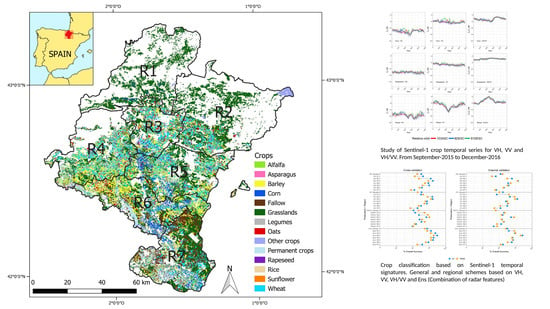
:Crop classification provides relevant information for crop management, food security assurance and agricultural policy design. The availability of Sentinel-1 image time series, with a very short revisit time and high spatial resolution, has great potential for crop classification in regions with pervasive cloud cover. Dense image time series enable the implementation of supervised crop classification schemes based on the comparison of the time series of the element to classify with the temporal signatures of the considered crops. The main objective of this study is to investigate the performance of a supervised crop classification approach based on crop temporal signatures obtained from Sentinel-1 time series in a challenging case study with a large number of crops and a high heterogeneity in terms of agro-climatic conditions and field sizes. The case study considered a large dataset on the Spanish province of Navarre in the framework of the verification of Common Agricultural Policy (CAP) subsidies. Navarre presents a large agro-climatic diversity with persistent cloud cover areas, and therefore, the technique was implemented both at the provincial and regional scale. In total, 14 crop classes were considered, including different winter crops, summer crops, permanent crops and fallow. Classification results varied depending on the set of input features considered, obtaining Overall Accuracies higher than 70% when the three (VH, VV and VH/VV) channels were used as the input. Crops exhibiting singularities in their temporal signatures were more easily identified, with barley, rice, corn and wheat achieving F1-scores above 75%. The size of fields severely affected classification performance, with ~14% better classification performance for larger fields (>1 ha) in comparison to smaller fields (<0.5 ha). Results improved when agro-climatic diversity was taken into account through regional stratification. It was observed that regions with a higher diversity of crop types, management techniques and a larger proportion of fallow fields obtained lower accuracies. The approach is simple and can be easily implemented operationally to aid CAP inspection procedures or for other purposes.
1. Introduction
Crop classification is one of the most important agricultural applications of remote sensing [1]. Knowing what crops are present in the fields is very useful both at a local and global scale [2]. For instance, this information is valuable for the design and implementation of agricultural policies [3], as well as for crop management and food security assurance [4]. Crop classification is also a pre-requisite for implementing other remote-sensing-based applications at the field scale (e.g., biomass and yield estimation, anomaly detection, etc.). Satellite Earth observations provide information about biophysical properties of the Earth’s surface and their spatial variability with a given revisit time. This constitutes a very rich information source that can be used for identifying the crop types being cultivated and for monitoring them along their growing cycle [5].
European farmers benefit from the Common Agricultural Policy (CAP) support of the European Union, which started back in 1962. CAP establishes different financing instruments including area-based payments and cross-compliance requirements (Regulation (EU) No 1306/2013). Competent authorities might check whether farmers’ declarations are correct (i.e., they are actually growing the crops they declare on each field and follow cross-compliance requirements). Traditionally, this has been done through field inspections on a sample of fields, constituting an expensive, inefficient and incomplete check system. On June 2018, the European Commission drafted the new modification of the CAP (Regulation (EU) 2018/746) regarding applications, payment claims and checks to be fully implemented in 2020. These modifications recommend the establishment of procedures to check and track all eligibility criteria using Copernicus Sentinels data or similar data. Therefore, several initiatives and research efforts are being conducted at present to fulfill this aim, including EU-funded projects like Sen2-Agri [6], RECAP [7] or SEN4CAP [8].
Indeed, the Copernicus program has been a game changer in this field of research, with frequent observations potentially useful for crop classification (both in the microwave (Sentinel-1, S1) and optical (Sentinel-2, S2) domain), which are acquired systematically over the world and freely distributed [9]. Their excellent compromise between spatial and spectral resolution, and above all, their enhanced revisit time, through the use of constellations of twin satellites (S1A–S1B and S2A–S2B), make them a unique solution for monitoring dynamic processes like vegetation growth at the scale of agricultural fields.
Until the Sentinels were launched, typical approaches for crop classification were mostly based on the evaluation of the spectral signature of crops obtained from multispectral imagery on key moments of the phenological cycle and their statistical (di)similarity [10]. However, early studies [11] already recalled that this approach might have limitations after observing that different fields of the same crop might have different spectral responses due to slight differences in the agricultural management calendar from field to field. In addition, different crops might expose a similar spectral response on a given date, thus, an examination of the multi-temporal evolution of the spectral response of a field was hypothesized as a potentially relevant information for crop recognition [11]. Yet, the unavailability of multi-temporal datasets with the sufficient revisit time (i.e., 16 days for Landsat) precluded the further development of this type of method until sensors such as MODIS became available [12,13]. With the availability of S2 data, similar approaches but with a higher spatial resolution have been developed [7,14,15].
In large parts of the world, remote sensing in the optical domain has been difficult to implement operationally due to persistent cloud cover limiting the number of viable observations along the agricultural season [16]. Synthetic Aperture Radar (SAR) sensors can be an interesting alternative for those regions since they can operate in cloud-covered and poorly illuminated conditions. In addition, SAR data provide complementary information to optical sensors, reflecting geometric and dielectric properties of vegetation and soil, which have been proven relevant for crop classification [17,18]. The first SAR-based crop classification experiences used a few single polarization scenes and generally achieved limited results [5], but soon after, several studies demonstrated that adding dimensionality through multi-frequency, multi-polarization or multi-temporal SAR observations increased the accuracy of crop maps [19,20]. Observation frequency determines the size of the scattering elements that contribute to backscatter [21], with short wavelengths (X-band) interacting with smaller canopy constituents (e.g., leaves and fruits) than medium (C-band, e.g., small branches and stems) or longer wavelengths (L-band, e.g., larger branches and trunks). The latter might also be more sensitive to soil surface roughness and moisture conditions below the canopy. Regarding polarization, quad-polarized data provided polarimetric features which are potentially interesting for classification and other agricultural applications [21,22]; however, dual-polarized configurations might be more efficient for multi-temporal large-area mapping and still provide interesting information for crop monitoring [23] and classification [24,25]. On the other hand, multi-temporal observations of single or dual-polarized backscatter have demonstrated a clear benefit on the accuracy of the resulting classifications [24], since morphological differences in some particular stages of the phenological development might be key for differentiating pairs of crops that are otherwise quite similar the rest of the year [18].
Given the actual availability of SAR constellation missions with an extremely short revisit time and high spatial resolutions, classification methods that explicitly exploit time series information have recently been developed with promising results. In effect, supervised classification schemes were developed based solely on time series information, where training data were used to obtain model time series for each class (i.e., temporal signatures) that were later compared with the elements to classify using some type of error metric. This way, Whelen and Siqueira [26] classified alfalfa, corn and wheat fields over a 10 km × 23 km area using L-band UAVSAR observations, and obtained accuracy values higher than 75% when HV backscatter, entropy or alpha time series were used. Later, using C-band Sentinel-1 data, this approach was refined with a case study over a portion of central North Dakota considering four crops (corn, soybean, wheat and grass/pasture) and obtaining an accuracy of 85% [27]. In a similar fashion, Xu et al. [28] classified two corn-dominated sites using Sentinel-1 time series, and obtained accuracies ~90%. In these studies, the error metrics used to compare the temporal signatures with the time series of the elements to classify differed, but only slight differences were observed in the obtained accuracies [28]. The performance of this classification approach was comparable to results obtained with machine learning algorithms. Yet, the simplicity and robustness of the approach makes it transparent, portable from season to season and resilient to crop growth anomalies. However, further studies were recommended to explore the performance of this approach on regions with a higher crop diversity [27] and more heterogeneous conditions.
Indeed, the number of crop classes considered strongly impacts the accuracy of the results obtained [24]. Typically, published crop classification studies based on SAR data considered six different crop classes or less [17,26,28], although some studies had a higher number—however, this was normally below 10 [25,29] or 15 [24,30]. Furthermore, some studies did not solely address crop classification, as they considered both crop categories and other land covers such as forests, water surfaces or urban areas [29]. Regarding the number of fields used for training and validation, the published studies differ greatly, although in many cases, they were below 100 [26,28] or 1000 [24,30]. Few published works considered near-operational applications with 10,000–100,000 fields or more and these used optical imagery [3,6]. In addition, the heterogeneity in terms of agro-climatic conditions of the area of interest and field sizes might impact the performance of the approach, as it has mostly been applied to rather homogeneous areas with large fields [26,27,28].
Therefore, the main objective of this study is to investigate the performance of a supervised crop classification approach based on crop temporal signatures obtained from Sentinel-1 time series on a challenging case study with a large number of classes and a high heterogeneity in terms of agro-climatic conditions and field sizes. Hence, the temporal signatures of all crop categories were interpreted and the confusion with other classes was evaluated. The study is framed on a real case study of crop identification for the aid of CAP inspections focused on the Spanish province of Navarre, a region of strong agro-climatic and geographic diversity with pervasive cloud cover. The region was stratified into different agro-climatic regions and different classification models were trained to evaluate the benefits of stratification. Thus, a specific objective of this study was to test whether the differences in crop growing conditions by agricultural region had any influence on the crop classification accuracy. Furthermore, the relation between field size and classification results was investigated. Special attention was also paid to the analysis of results obtained with classification models based on different sets of input data, comparing VH and VV polarizations, but also the VH/VV ratio and implementing an ensemble approach that jointly considered VH, VV and VH/VV temporal signatures.
2. Materials and Methods
2.1. Study Area
The study area covers the agricultural areas of the province of Navarre (Northern Spain). This province has an extension of 10,391 km2 and it is characterized by its landscape and climate diversity. The Northern area is mountainous, and wet and forests and grasslands are predominant, while the Southern area is dryer and constituted mainly by extensive plains of the Ebro basin, where the proportion of arable land is higher with both irrigated and rainfed agriculture. Between these two areas, there is a transition zone with mixed characteristics. Due to this diversity, Navarre is stratified in seven agricultural regions with distinct agro-climatic conditions [31] (Table 1).
Different types of crops are grown in each region. Grasslands prevail in northern regions (1 and 2). Winter cereals are found throughout the whole province, while other winter crops, such as legumes and rapeseed, are common only in central regions (3 and 4). The diversity of crops in southern regions (6 and 7) is larger, where alfalfa, corn, asparagus, horticultural crops and permanent crops are also widespread. Corn, the most common summer crop, is mainly grown under irrigation systems, except in Region 1, where the high amount of precipitation allows rainfed cultivation. Other summer crops cultivated in Navarre are sunflower, found in every region, and rice, only grown in southern regions. It is important to mention that the proportion of fallow fields varies strongly depending on the region, being particularly high in Southern Navarre, especially in region 7.
2.2. Sentinel-1 Data
The SAR data used in this study were Sentinel-1 C-band Interferometric Wide (IW) swath mode images downloaded as level-1 Ground Range Detected (GRD) products. All available Sentinel-1 images covering the study area from 1 September 2015 to 30 December 2016 were acquired (Figure 1). The images belonged to three relative orbits: one ascending node and two descending nodes (103ASC, 8DESC and 81DESC). Yet, only the 103ASC relative orbit covered the entire area of Navarre, whereas the descending nodes excluded a small area of the province from the image, specifically the Western part in 8DESC and the Eastern part in 81DESC (Figure 2).
The images were processed using SNAP Sentinel-1 Toolbox following these steps: (1) thermal noise removal; (2) slice assembly; (3) apply orbit file operator; (4) calibration to β0; (5) speckle filtering; (6) terrain-flattening; (7) range-doppler terrain correction and (8) subset to the extent of Navarre. The speckle reduction was performed using a 3 × 3 window Gamma-MAP filter. The SRTM 1sec HGT DEM was used for terrain-flattening and terrain correction. After these corrections, terrain-flattened γ0 backscatter coefficient values were obtained. The results of this process were 110 images with three channels each: two backscatter coefficients (VH and VV) and their ratio (VH/VV) in dB units. The pixel size of the final products was set to 20 m. All the images corresponding to the three relative orbits were stacked according to their time.
2.3. Ground Truth and Data Extraction
Ground truth information for training and validation was extracted from a geographical database containing field boundary polygons for EU Common Agricultural Policy (CAP) declarations (335,094 polygons) and inspections (21,850 polygons) for the agricultural year 2016. This database was provided by the Agriculture Department of the Government of Navarre (information not publicly available). Field inspections were carried out from June to August 2016, as part of the verifications of CAP subsidy declarations.
The geographical database was refined as follows. A 5 m inside buffer was applied to the agricultural field boundaries in order to avoid mixed pixels that could contain information from different crops. Fields smaller than 0.5 ha were masked out in the declarations dataset. In the inspections dataset, the mask was less restrictive, leaving out fields that contained less than 6 pixels. Then, field statistics were computed, obtaining the median, mean, minimum, maximum and standard deviation backscatters values for the S-1 channels. For each field, a temporal signature with the information of the three relative orbits was obtained. Fields not covered in one of the descending orbits had missing values for those specific dates. Finally, the crops were grouped into 14 classes: alfalfa, asparagus, barley, corn, fallow, grasslands, legumes, oats, other crops, permanent crops, rapeseed, rice, sunflower and wheat.
At most, 10% of farmers’ declarations are expected to be wrong due to errors, fraud etc. [32]. These wrongly declared fields could affect the training phase by introducing erroneous information in the learning process of supervised classification algorithms. In order to minimize the impact of wrongly declared parcels in the declarations dataset, the 10% of fields whose median backscatter temporal signature differed the most with the median signature of its declared class in each region was discarded. The median was chosen to further reduce the effect of speckle inside the field. The comparison between the temporal signature of the crop and that of each field was based on the R2 metric. The final number of fields in Navarre is shown in Table 2 and Figure 3 (see Supplementary Materials for the number of fields per region: Table S1).
2.4. Separability Analysis
As a preliminary step, a feature importance analysis was conducted comparing the statistical features calculated for the different polarizations. For this analysis, the Jeffries–Matusita (JM) distance was evaluated [33], which provides a measure of separability between pairs of classes and has been identified as a good indicator of crop separability [34]. The JM distance between a pair of probability distributions is given by the following:
where JMij is the JM distance between a pair of classes ωi and ωj, x is the feature observed (field backscatter statistics) and p (x|ωi) and p (x|ωj) are the conditional probability functions for x given ωi and ωj, respectively. JM distance values range between 0 and 2, with higher values indicating higher separabilities between pairs of crops.
The JM distances were calculated per date for each pair of crops, for the different polarizations and for the different statistical features. A mean JM distance value was calculated for the whole period of study, averaging the distances obtained for each date. This mean JM-distance was used to compare the importance of the different polarizations and statistical features calculated. Two statistical features obtained the highest separabilities: the mean and the median. The median was chosen for the classification because of its higher robustness to outliers.
2.5. Classification
A supervised classification algorithm based on the temporal signatures of crops was applied. The algorithm is similar in concept to the one used in Whelen and Siqueira [26,27] and Xu et al. [28]. However, there are some significant differences in the way similarity is measured (see below). The basic concept behind this classification algorithm is that crops exhibit physical differences during the growing season due to their phenological development, which leads to different backscatter time series. Thus, the characteristic time series of each crop, as observed by Sentinel-1, is referred to as its temporal signature. This concept of temporal signature somehow mimics the idea of the spectral signature of a crop, i.e., the typical reflectance response of a crop with respect to wavelength. Therefore, we could define the temporal signature as the typical backscatter response of a crop with respect to time. The basic hypothesis is that these temporal signatures are representative of each crop and can be used to identify whether an unknown field belongs to one class or another. In the training phase, the temporal signatures of each crop class were obtained following a three-fold cross-validation scheme using the declarations dataset, where 2/3 of the ground truth samples were used for training and the remaining 1/3 for validation, in three successive random folds. Backscatter time series were formed by adding the information obtained at the three relative orbits used. After this training phase, each field was classified by comparing its temporal signature one by one with the different crop temporal signatures. In fact, each field was assigned to the class providing the best fit between its temporal signature and the crop temporal signature. To quantify the best fit, two variants were explored, the first variant assumed the best fit as the one with the lowest root mean squared error (RMSE), and the second as the one with the highest determination coefficient (R2). This differed from related studies; Whelen and Siqueira [26,27] used a normalized error metric and Xu et al. [28] used a spectral similarity measure. Here, an error metric (RMSE) and a correlation metric (R2) were evaluated, as they provide a complementary way to quantitatively compare two curves. Since the crops can have different calendars, the duration of the curves to be compared was adjusted to each crop type (Table 3). In addition, each crop could be characterized by three different temporal signatures depending on the channel used: VH, VV and VH/VV. Thus, three different classification schemes were applied by considering these channels individually. One additional scheme was explored by considering the similarity to the three polarizations conjointly and named as the ensemble scheme (Ens). Therefore, in total, eight variants were explored (four input features × two goodness-of-fit measures).
In order to test whether the differences in crop growing conditions by agricultural region had any influence on the crop classification accuracy, the supervised classification algorithm was fitted at different spatial extents: first, for the whole province of Navarre, and second, stratified for each of the seven agricultural regions. In the first case, the temporal signatures were obtained for the whole province, whereas in the second, specific temporal signatures per region were obtained.
For each classification scheme, the accuracy was assessed through a confusion matrix whereby the Overall Accuracy (OA) was calculated, as well as each crop’s Producer’s Accuracy (PA), User’s Accuracy (UA) and F1-score (the harmonic mean between PA and UA). In fact, a two-level accuracy assessment was implemented. The first level corresponded to the three-fold cross-validation and used the 1/3 ground truth data set left out for validation on each of the three-folds. Additionally, a more rigorous second level validation was performed based on the field inspections dataset available, called external validation. This second dataset was obtained through field visits, thus, its reliability is believed to be higher. However, the sampling did not follow the standard recommendations for accuracy evaluation [35], and had a higher proportion of fallow, permanent crops and other crop classes (Table 2), categories that can be more difficult to classify than others such as grasslands with a much lower number of samples. This might negatively impact the OA values obtained. In addition, the size of fields was smaller compared to the declarations dataset (Table 2). Therefore, the results should be interpreted bearing this point in mind. The accuracy metrics for these two validation levels were reported in the results. Due to the small size of several fields in the external validation dataset, accuracy results were also reported and analyzed by field size considering three size groups: (1) <0.5 ha; (2) 0.5 ha–1 ha; (3) ≥1 ha.
3. Results
3.1. Separability Analysis
Table 4 shows the results for the statistical features importance analysis, where the mean JM distances for all pairs of crops was calculated. The standard deviation time series obtained the lowest values, while the mean and median achieved the highest JM distances, and were very similar. As indicated in Section 2.4, the median time series was selected for computing the temporal signatures of each crop class due to its higher robustness to outliers.
The separability values between each pair of crops for the median time series are represented in Figure 4. Although the values are, in general, low (<1), it must be pointed out that this is an average value for the whole period of study, thus, they should be used for comparison between crop pairs and polarizations. There were pairs of crops that obtained similar values (in most cases low) for the three polarizations. In VH polarization, rapeseed and rice had relatively high separabilities with most of the crops. In VV, alfalfa was the crop with the highest values, followed by oats and barley. In the case of VH/VV, the highest separabilities were achieved when comparing winter versus summer crops.
The temporal evolution of crop separability provides interesting information on the time periods that contribute the most to crop identification (Figure 5). Monthly boxplots of JM distances for all crops show that in general the period between March and August provided the highest separabilities for the three polarizations (Figure 5a–c). When evaluating the separability between winter crops (barley, legumes, oats, rapeseed and wheat), both VH and VV polarizations had rather high values in spring months, while VH/VV distances were considerably lower (Figure 5d–f). In the case of summer crops (corn, rice and sunflower), separabilities were lower than for winter crops, yet they increased between May and August for VH and VV polarizations, and between July and November for VH/VV (Figure 5g–i). Permanent crops had in general low separability values throughout the whole period, taking slightly higher values in winter months for VH and VV polarizations, and in spring for VH/VV (Figure 5j–l).
3.2. Temporal Signatures of Crops
Figure 6, Figure 7 and Figure 8 represent the temporal signatures of the studied crops for the three backscatter channels (VH, VV and VH/VV) from 1 September 2015 (day 0) to 30 December 2016 (day 487). Generally, the signature of each crop in the different regions was similar, thus, a general description is provided and the regions where the response differed are pointed out (see Supplementary Materials for detailed temporal signatures per region: Figure S1). For each polarization, the temporal curves of the three relative orbits had similar backscatter values and the trend was the same throughout the whole period of study. In the following sections, the temporal signatures are commented on by crop type.
3.2.1. Winter Crops (Barley, Legumes, Oats, Rapeseed and Wheat)
Winter cereals (barley, oats and wheat) are normally sown between October and November, with the exception of Region 7, where short cycle varieties of barley and wheat are also sown in January and February. Harvest takes place normally during June and July, starting earlier in the most southern regions. VH/VV signatures of winter cereals responded positively to the growth of vegetation along the season until the ripening stage (Figure 6), which occurred in May (~250 day) for barley and in June (~275 day) for wheat and oats. Then, during senescence, VH/VV values decreased until the crop was harvested. It is possible to identify in the signature of barley that harvest occurred earlier than in wheat or oats (Figure 6).
VH and VV temporal signatures were very similar for the three cereal crops during autumn and winter, with no clear trends and a strong variability between successive dates. In April (~200 day), a consistent decrease in backscatter was initiated in both polarizations, being sharper in VV. After ~250 days, backscatter values increased again. In this phase, barley increased more than wheat and oats. During senescence, VH values in the three cereal crops and VV in barley decreased steadily until the harvest was finalized. The temporal signatures of cereals showed the same trends in all agricultural regions, except for Region 7, where VH and VV backscatter signatures were noisier (Supplementary Materials: Figure S1).
The legume crops cultivated in Navarre are mostly beans and peas. These crops, which are intended for fodder in the majority of the region, are grown from October to July. In this case too, VH/VV responded positively to crop growth (Figure 6). Regarding VH, an increase in backscatter values was detected from the end of autumn due to the development of the crop. The onward increase of backscatter finished in June (~275 day), and was followed by a decrease due to crop senescence. In the case of VV, there was not a clear trend until March (~200 day), when backscatter started growing smoothly until June. VH backscatter values grew slowly in winter and early spring. There was a stronger increase from April (~215 day) to June (~275 day). After this peak, the values dropped, matching the senescence period. The temporal signatures of legumes were shorter in Region 7 (see Supplementary Materials: Figure S1). In this region, the increase of the curves came later—at the end of March—and the slope of the decreasing curves was steeper.
Rapeseed is mostly grown in the central area of Navarre. Its agricultural calendar is similar to that of winter cereals, with sowing in September and harvest in July. VH/VV signatures followed the growth of the crop along the cycle, reaching their highest peak in May (~250 day) (Figure 6). VH backscatter values of rapeseed increased since the beginning of the cycle, but there was a steeper increase between the end of April (~240 day) and the peak at the end of May, coinciding with the inflorescence emergence. After this peak, VH backscatter dropped significantly until mid-July, when the crop was finally harvested. In the case of the VV signature, no clear trend was apparent until mid-April (~230 day), when the values first decayed and then suddenly increased, depicting a peak similar to the VH curve.
3.2.2. Summer Crops (Corn, Rice and Sunflower)
These three crops are usually sown in April; thus, the variability of the time series before this date was high in all cases (see the interquartile ranges in Figure 7). Harvesting of sunflower occurs around September before cereal is sown, as it is a common crop for cereal rotations. Rice and corn harvest dates can range from October to December.
Looking at VH/VV time series (Figure 7), the temporal signature responded positively to the growth of corn and rice, but for sunflower, it was not as evident, particularly in the descending orbit curves. For this crop, backscatter values increased both in VH and VV from the beginning of June until August. In this case, VH/VV did not adequately resemble crop growth. In corn, there was an increase in VH backscatter from plant emergence until July. After that moment, there were no clear trends. Corn VV series did not show any clear trend during the growing cycle. Rice is flooded before sowing, and this caused an evident effect in VH and VV time series. There was an increase in backscatter at the beginning of April, coinciding with soil tillage, followed by a strong decrease due to the specular reflection caused by standing water in the fields. Once the crop started to grow, backscatter also increased steadily until August (~336 day). After that point, VH backscatter continued increasing until the end of the period of study, whereas VV remained steady till November (~400 day), when it started to grow. It is remarkable that the VH/VV time series of corn were all similar throughout the different regions, except for the northern regions, which were shorter than the rest (see Supplementary Materials: Figure S1).
3.2.3. Rest of Crops (Alfalfa, Asparagus, Grasslands, Permanent Crops, Other Crops and Fallow)
Alfalfa is a crop that can be sown in different periods of the year (September or spring months), whose management normally includes irrigation and several cuts throughout the cycle. These cutting events complicate the interpretation of the crop signature since different fields might be cut on different dates, resulting in a poorly informative average curve. Yet, although VH and VV temporal signatures showed different peaks during the period of study, the values remained relatively constant. A small increase in VH/VV was observed from January to May.
Asparagus follows a cycle of two years. This crop is planted between February and April of the first year, and harvested between March and May of the second year. VH and VV temporal signatures showed many backscatter peaks along the period of study. It is possible to detect an increase of VH from May to November, the period of vegetative growth (Figure 8). VH/VV also augmented in this period, although it increased very smoothly.
Backscatter signatures of grasslands were heterogeneous and did not follow any defined pattern (Figure 8). In this case (as in alfalfa), the influence of individual cuttings complicated the interpretation of the temporal signature.
Permanent crops are another heterogeneous group including different woody crops: vineyards, olive trees, almond trees and different types of fruit trees. In VH and VV curves, there were backscatter peaks that were smoothed during spring and summer. VH/VV slightly increased from mid-spring until mid-autumn.
The great variability of crops included in the “other crops” class was clearly visible in the dispersion of the class’ temporal signature (Figure 8). This class included herbaceous and horticultural crops with both summer and winter cycles. There were no clear trends and the interquartile range was large throughout the period of study.
Fallow temporal signatures also had high interquartile ranges. For all the three polarizations, there were no clear trends, with different peaks along the period of study.
3.3. Classification Results
3.3.1. General Results
Overall Accuracy (OA) results showed differences among regions, polarization channels used as input, best fit metric and type of validation (cross-validation or external validation) (Figure 9). The best classification results were achieved in Region 3 in cross-validation, using Ens as the input and R2 as the best fit metric, with OA higher than 85%. On the other hand, using only VH/VV as input and R2 resulted in the poorest results, with an OA of around 50% in specific regions. In Figure 10, the classification map obtained with the best configuration (Ens scheme using R2 as the best fit metric) is represented.
External validation provided systematically lower OA values than cross-validation, with the exception of Region 3, where the results were very similar. Although the accuracies were lower in the external validation, it can be observed that the results followed a similar distribution to the cross-validation output (Figure 9). In the following sections, the cross-validation results will be analyzed (see Supplementary Materials for the detailed external validation results).
3.3.2. Input Features and Goodness-of-Fit Metrics
OA results showed that classifications based on single polarization channels did not reach satisfactory results (Figure 9). VH and VV channels achieved similar accuracies in each region individually (at best 80% OA), while classifications using the VH/VV ratio as the input obtained lower values (at best, 75% OA). On the other hand, considering all the available input features (Ens in Figure 9) yielded the best results for all the regions, reaching 87% of OA in Region 3.
Regarding the goodness-of-fit metric used for classification, R2 obtained the best results for VH, VV and Ens, while RMSE was the best for VH/VV. Although R2 achieved the best global results for the most favorable schemes (Ens), there were differences among crop classes. As is shown in Table 5, legumes, oats, rapeseed and rice achieved an improvement of the F1-score between 6% and 18% when RMSE was considered. On the other hand, alfalfa, fallow, grasslands and permanent crops obtained better results when R2 was used. Asparagus, barley, corn, sunflowers, other crops and wheat did not present large differences between one metric and the other.
3.3.3. Results per Region
Regarding the classification results for the different regions, the OA values varied strongly. Focusing on the Ens approach with R2 as the goodness-of-fit metric (Figure 9), Region 3 obtained the highest accuracies (OA = 87%). The accuracies in Region 2 were also good (i.e., 84%). Region 4 and 5 also had good OA results—around 80%. In Region 1 and Region 6, the OA results yielded 78% and 74%, respectively, whereas the worst OA results were achieved in Region 7 (64%).
Table 6 shows the increment in crop accuracy (PA, UA and F1-sore) when the regional results were compared to Navarre’s results. The regional accuracies were extracted from a confusion matrix built by adding the individual confusion matrices of each region (Supplementary Materials: Table S2). This matrix allowed for an easy comparison of whether the stratification of the province in agricultural regions improved the general classification results. PA, UA and F1-score results were higher for the stratified case, with the exception of PA- and F1-score of fallow, which decreased by 2% and 1%, respectively, UA of grasslands decreased by 3% and PA of rapeseed decreased by 1%. In total, OA increased from 72% to 77%.
3.3.4. Results per Crop
In the following section, the results per crop are provided, reporting the Ens and R2 classification scheme for Navarre (Table 7) (for the rest of schemes, see the Supplementary Materials: Table S2 and Figure S2). Interesting results related to polarization channels and fit metrics are also reported.
Winter Crops (Barley, Legumes, Oats, Rapeseed and Wheat)
Barley is the crop that achieved the best classification results, with F1-score of 87% and balanced PA and UA results (Table 6). The F1-score of wheat was 71%, with higher UA than PA (84–69%, respectively) (Table 6). On the other hand, oats obtained poorer classification results, with an F1-score of 42%. Although PA was relatively high (70%), UA was low (30%), due to many wheat fields being incorrectly assigned to oats (Table 7). In general, the results obtained per region were similar (Supplementary Materials: Table S2 and Figure S2). Region 2 and Region 3 achieved the highest PA, UA and F1-score for the three cereal crops compared with other regions. In Region 1, although most barley fields were correctly classified, the F1-score was worse due to the incorrect assignment of grasslands fields to the barley class. The lowest classification accuracies of winter cereals occurred in Region 7, where other crops were also misclassified as barley and wheat, and many fallow fields were incorrectly classified as winter cereals.
Legumes obtained an F1-score of 47%, with a higher accuracy in PA than in UA (70% and 35%, respectively) (Table 6). Incorrectly classified legumes fields were assigned mainly to the rapeseed class (Table 7), and in a lower proportion, to winter cereals, grasslands and fallow. On the other hand, some grasslands, winter cereals (barley and wheat), fallow and other crops fields were wrongly assigned to legumes causing low UA values (Table 6 and Table 7). In the case of the different regions, the values of PA were also higher than UA for legumes (Supplementary Materials: Table S2 and Figure S2). The low values of UA were mainly due to incorrectly classified grasslands and in some regions (6 and 7), fallow fields. The exception was Region 3, where both PA and UA scores were high, achieving an F1-score of 89%.
Rapeseed fields reached high PA (99%), while UA was not as good (59%), leading to an F1-score of 74% (Table 6). The fields wrongly assigned to rapeseed belonged principally to legumes, other crops, barley and fallow classes (Table 7). Per region, UA values were higher than in Navarre (Supplementary Materials: Table S2 and Figure S2), reaching high values of F1-score, especially in Region 3 (97%). The exception was Region 6 (UA = 20%), due to the lower number of rapeseed fields and the incorrect assignment as barley, legumes and fallow fields.
Summer Crops (Corn, Rice and Sunflower)
The accuracy values of summer crops in Navarre were variable (Table 6). Rice fields were mostly correctly classified, reaching a PA of 99%, UA of 74%, and an F1-score of 84% (Table 6). Corn had an F1-score of 78%, with balanced PA and UA values (75% and 81%, respectively), and some confusion with asparagus and other crops fields. Wrongly assigned fields to corn were mainly the other crops class. Sunflower was the summer crop with the worst results (F1-score of 55%, PA of 87% and UA of 41%), with confusion with other crops and fallow fields, causing these low UA values (Table 7).
Rice, which is only present in Regions 6 and 7, achieved slightly higher accuracies when the classification per regions was considered, with F1-scores of 90% and 93% for Regions 6 and 7, respectively (Supplementary Materials: Figure S2). In the case of corn, the classification was highly accurate in Regions 3 and 5 (F1-scores of 96% and 93%). In Regions 6 and 7, where the majority of corn fields were found, the F1-scores were also good (around 83%). Yet, in Regions 1 and 2, the UA was much lower, mostly due to confusion with grasslands. In Region 4, UA values were not high (43%) due to the small number of corn fields. Sunflower repeated the patterns of Navarre in the different regions, with lower UA values compared to PA values, except in Region 3, where, again, both PA and UA were high (100% and 91%) (Supplementary Materials: Table S2 and Figure S2).
Rest of Crops (Alfalfa, Asparagus, Grasslands, Permanent Crops, Other Crops and Fallow)
The classification of alfalfa fields achieved an F1-score of 48%, with higher PA (74%) than UA (35%) (Table 6). PA’s errors were mostly due to being wrongly assigned to legumes, while UA values were impacted by confusion with grasslands, permanent crops and fallow (Table 7). In Regions 6 and 7, where alfalfa is most frequent, the results were similar (Supplementary Materials: Table S2 and Figure S2).
Asparagus was one of the crops with the poorest classification results, with an F1-score = 25%, PA = 60% and UA = 16%. Many fields belonging to the class permanent crops were classified as asparagus and, in a smaller proportion, corn and other crops (Table 7). These incorrect assignments were even higher than the actual number of asparagus fields, which explained the low UA. Similar results were obtained per region (Supplementary Materials: Table S2 and Figure S2).
Grasslands was the largest class in the declarations dataset. The classification had higher UA values (92%) than PA (71%), achieving an F1-score of 80% (Table 6). Although PA was not low, wrongly classified grassland fields impacted the UA of many different crops due to their higher proportion (Table 7). The main errors in PA were due to the confusion with other crops, legumes, alfalfa and permanent crops. Per region, similar results were obtained, except for Regions 6 and 7, where results were worse (F1-scores below 70%) (Supplementary Materials: Table S2 and Figure S2).
The class permanent crops obtained intermediate accuracies (PA = 65%, UA = 72% and F1-score = 68%). The main error in UA was related to incorrectly classified grasslands and fallow fields, while PA was affected by the confusion with asparagus class. Similar results were achieved per region (Supplementary Materials: Table S2 and Figure S2), with the exception being Region 3, where UA dropped to 29%.
Other crops was the class that was worst classified, with F1-score = 12%, PA = 13% and UA = 12% (Table 6). In all the regions, the results were also poor, and confusion occurred with many different classes, i.e., grasslands in northern regions, and permanent crops and fallow in southern regions.
Finally, fallow classification achieved better UA than PA (88% and 58%, respectively) and had an F1-score of 70%. The wrongly classified fallow fields were assigned to many different crop classes, but particularly to legumes, barley, other crops and grasslands. In contrast, in Region 1, the classification results were poor (F1-score = 2%), while in the rest of the regions, results were similar to those of the whole province.
3.3.5. Influence of Field Size
In most of the classification schemes and regions, the OA values obtained were higher for large fields in comparison with small ones. In some cases, the difference between small (<0.5 ha) and large fields (>1 ha) was higher than 14% (Table 8).
Regarding the results per crop, it can also be observed that, in most cases, F1-score values were higher for large- and medium-sized fields, in contrast to smaller fields (Figure 11). This was particularly true for fallow and rice classes, where the accuracies were considerably higher for large fields than for small ones.
4. Discussion
4.1. Crop Classification Results with Regard to Its Temporal Signatures
This study implemented a supervised classification technique based on the temporal signature of crops to a CAP inspection case study on a region with strong agro-climatic diversity. The results obtained varied significantly from crop to crop, with the crops that exhibited any singularities in their time series being the best classified. Cereals, and in particular, wheat and barley, are the most common crops in the region, and showed quite a distinctive temporal signature with a strong decay in backscatter in the stem elongation phase, where surface scattering from the soil was progressively attenuated by growing cereal stems [36]. This decay was particularly strong in VV, due to the vertical arrangement of stems through the so-called differential attenuation mechanism [37,38]. This characteristic decay was followed by an increase in backscatter due to the structural changes experienced by the canopy during the heading stage [23,37,39,40]. At this moment, a strong and well-defined peak occurred in VH and VV barley time series, probably due to the bending of barley spikes at this phase [38,39], which did not occur in wheat and oats that maintained a vertical geometry. From ripening to senescence and harvest, cereal canopies dried-out and a greater penetration [41] and a higher influence of the soil surface [37] was observed. The unique backscatter pattern of barley allowed a successful identification with F1-scores of ~85%. Wheat was also adequately identified (F1-score of ~76%), although was sometimes confused with oats, which was the cereal crop with the poorest results (F1-score of ~50%).
The architecture of legumes and rapeseed canopies is completely different from cereals, with heterogeneous shrub-like structures that produce volume backscatter [39]. This is the reason why VH and VV time series were so different from cereals, although the period of cultivation was the same. Unlike cereals, rapeseed and legumes’ curves in VH started increasing right after the germination of the crop, due to the volume scattering produced by plants [38,42,43,44]. This behavior changed suddenly for rapeseed at the period of pod formation after flowering, producing a strong peak in VH (and to a lesser extent in VV). In VV, just before this peak, a small backscatter decrease was observed coinciding with the start of flowering, as also reported by Wiseman et al. [45] and Veloso et al. [23]. Ripening and senescence produced a strong decrease in VH backscatter (and to a lesser extent in VV) due to canopy drying and a reduction of the volume scattering component. This decrease occurred for both rapeseed and legumes, although it was much greater for the former. Accordingly, classification results were successful for rapeseed (F1-score of ~75%) but worse for legumes (F1-score of ~50%), whose temporal signature was confounded with other crop classes.
Summer crops also achieved good classification results. Corn, with an F1-score of ~75%, was characterized by a rather insensitive VV curve, and on the contrary, a clear increase in VH due to volume scattering during the vegetative growth phase (250–300 days) until the plants reached their maximum height [46], after which it remained rather constant. Rice achieved an F1-score of ~85%, mainly due to its characteristic time signature due to flooding at the time of sowing, which led to very low backscatter due to specular reflection [47]. After rice emergence, VV increased rapidly due to double-bounce scattering, followed by a subsequent increase in VH polarization caused by volume scattering from the rice canopy that went on until the end of the season. Sunflower was the summer crop with the poorest F1-score (~60%), but this was not expected due to its rather unique temporal signatures exhibiting both VH and VV sensitivity to crop growth in the stem elongation phase where most vegetative growth occurred (250–400 days). The structure of sunflower, with broad leaves and thick stems with large open spaces between plants, caused both volume and double-bounce backscatter [48]. Sunflower fields were mostly correctly classified (PA > 85%), but a significant number of grasslands, fallow and other crops fields were incorrectly assigned to sunflower, leading to low UA values.
Asparagus, although having a biannual cycle, had a backscatter behavior similar to summer crops, with an increase in VH in summer (250–400 days) coinciding with the period of vegetative growth. Bargiel et al. [49] observed an increase in VV backscatter at X-band for this crop during summer, but our data at C-band showed a rather constant VV response. Classification results for asparagus were poor (F1-score of ~25%), mainly due to the incorrect assignment of corn and grasslands fields to asparagus (UA ~20%).
Some categories have a large variability in terms of management or species compositions. For instance, grasslands, alfalfa and fallow are classes where agricultural practices can vary significantly. Grasslands can range from an intensified management (in terms of soil preparation, sowing, fertilizing and mowing) to extensive rangelands that behave more like permanent covers and are only grazed in summer season. Fallow fields can also vary significantly depending on the management applied to spontaneous vegetation, i.e., it might be left to grow or it might be removed either chemically or mechanically. Alfalfa is a forage crop that is mowed several times throughout the season. However, the exact mowing dates might vary significantly from field to field, thus, the mean temporal signature might not be informative for this crop, showing a high variability during the season (the same applies for grasslands and fallow). Surprisingly, classification results were not as poor as expected given the rather unspecific temporal signatures of these crops. The three categories achieved quite good PA values (~70% for alfalfa and grasslands and ~60% for fallow), and UA values were high for grasslands and fallow but low for alfalfa. In fact, a significant amount of grasslands and fallow fields were incorrectly assigned to alfalfa causing its UA to fall. Altogether, such high variability categories should be better addressed by designing field-specific strategies (not based on median class signatures), such as those based on the multitemporal interferometric coherence [50].
Permanent crops was another heterogeneous class including vineyards, olives and other fruit trees, yet its classification was not too bad (F1-score ~70%). In this case, soil backscatter was predominant due to the open spaces between trees. Thus, during the period of study, the backscatter values presented peaks without a clear increasing or decreasing pattern, probably responding to soil moisture dynamics. Li et al. [51] also found a stable VH signal throughout the year in almond and walnut trees. During spring and summer, backscatter variations in VH and VV were smoothed, probably due to slower soil moisture dynamics at this time of the year, and because the growth of leaves during this period attenuated soil backscatter.
However, the worst results were obtained by the other crops class, a very heterogeneous category composed of a range of different minor crops, with both summer and winter cycles. Again, in this case, temporal signatures did not show any clear pattern, and in turn, its variability was very large, particularly in summer months. As a result, F1-scores dropped down to ~10%, and other crops fields were confounded both with summer (i.e., corn and sunflower) and winter crops (i.e., wheat and legumes). A redefinition of this class (e.g., splitting it into two more specific categories), could lead to an improved classification of this class, but also to higher UA values for other classes that were mistaken with it.
4.2. General Results
Previous research recommended multi-temporal optical data as the primary source for crop classification [52], reporting overall accuracies ~12% higher when optical data were used instead of SAR data. Indeed, crop classification approaches based on optical data provided typically accuracies above 75%, as long as imagery acquired in key phenological stages were available [3,6,15,53]. Yet, optical and SAR data provide complementary information that when combined might result in enhanced classification results [54]. However, when cloud conditions limit the viability of optical data, SAR observations still provide useful information [4,26]. The classification results obtained here were considered successful given the number of crop classes considered, the large number of fields classified and the agro-climatic diversity of the territory.
In this study, the configuration using the three S-1 features as the input (Ens) obtained the best results. For most crops, VH/VV responded positively to crop growth from emergence to senescence. Previous studies already identified VH/VV as a notable indicator of crop development correlated with fresh biomass [23] and plant height [55]. Yet, this information was very similar for crops of the same season and did not enable their separation. Therefore, VH/VV might differentiate when a field is vegetated or not, and even the start and end of the growing season, but crops with different morphological structures might produce very similar VH/VV temporal signatures. On the contrary, VH and VV polarizations provided diverse time series depending on different backscattering mechanisms and phenological events of the crops, and thus were more useful for crop classification. In each phenological stage, the structural characteristics of vegetation elements (size, shape, density, orientation) can vary [51], but also their water content and dielectric properties [41], in particular in the senescence phase [23,26]. VH and VV were useful to identify cereal heading [56] and rapeseed pod filling. Regarding backscattering mechanisms, VH was sensitive to volume scattering (e.g., in legumes, rapeseed, corn and sunflower) [26,51], and can be used as a vegetative growth indicator for these crops [57]. On the other hand, VV polarization was sensitive to surface scattering and its attenuation by cereals in the stem elongation phase [17,37], and also to double-bounce effects on sunflower [48] and rice [58]. Rice flooding was also easily detected in both VH and VV [58]. During the rest of the year, the main drivers of backscatter dynamics were meteorological events, soil preparation practices and harvesting procedures [26].
4.3. Influence of Field Size
Classification results were clearly influenced by the size of the fields, with fields >1 ha showing an OA improvement of ~14% when compared to small fields (< 0.5 ha). Similar results were already reported in the recent literature [6], showing that the operational applicability of crop-type mapping based on imagery with a spatial resolution of ~20 m in regions with very fragmented landscapes requires further advances to address the small field issue.
4.4. Regional Stratification
In general, our results improved when the classification algorithm was trained and applied separately to the different agricultural regions, with increments of ~5% in the OA and stronger improvements (10%) in the F1-score for particular crops such as alfalfa, legumes and asparagus. In our case, small and homogenous regions with a rather reduced crop legend and a small proportion of “difficult” categories (other crops, fallow, etc.) obtained the best results (i.e., Region 3). In turn, regions with a larger crop diversity, a higher proportion of fallow fields and more variability in crop management techniques obtained poorer results. In particular, southern regions (Region 6 and Region 7), due to their dryer climate, had a mix of rainfed and irrigated agriculture leading to a larger crop variety (including a higher proportion of other crops and fallow fields), more variable temporal signatures and poorer classification results. This occurred for categories such as winter cereals or legumes, where both long and short cycle varieties coexisted, some of them were intended for forage and some for human consumption. Corn was another category that improved after regional stratification, due to its diversity, with a shorter cycle rainfed corn for fodder production in Region 1 and a longer cycle irrigated corn for grain production in the rest of the province. Altogether, the results of this study showed that in geographic areas with great agro-climatic diversity, crop temporal signatures might change significantly; therefore, operational classification approaches should be applied to stratified regions with less variability.
4.5. Methodological Aspects
Some other methodological details were found to have an influence on the results obtained. First, the use of either R2 or RMSE as the metric for finding the best matching category did not provide consistent results in all cases. In general, the best classification strategies were those using R2. However, we found that RMSE provided the best results when VH/VV was the only input feature used, whereas R2 was better for VH, VV and Ens. The different shape of their temporal signatures (with smoother dynamics for VH/VV) could be behind these differences. Analyzing the results per crop, it was found that oats, rapeseed, legumes and rice obtained significantly better results with RMSE (6–18% improvement in F1-score) when the Ens configuration was used. In contrast, alfalfa, permanent crops, grasslands and fallow had higher F1-scores with R2, and for some cases, differences were minor (e.g., asparagus, barley, corn, sunflower or wheat). R2 might be more insensitive to class variability, with fields with slightly delayed phenology still having high R2 values, as long as they show a similar trend. Furthermore, RMSE might be more sensitive to the actual backscatter values and to abrupt changes in the time series due to particular phenological events or soil moisture variations.
4.6. Future Research
In this study, the duration of the time series was adjusted to the seasonality of the crops to be compared (winter, summer and permanent crops). This aspect was crucial due to the negative influence of the periods without vegetation cover on the variability of the time series. During autumn and winter months, differences in soil preparation dates and techniques (particularly important in furrowed crops such as asparagus) and soil moisture dynamics responding to wetting and drying events [23] are the main backscatter drivers because vegetation is still short. Furthermore, in the case of summer crops, during this period, spontaneous vegetation might show false dynamics that confound crop recognition. After harvest, some fields might exhibit regrowth of natural vegetation, while some others might be quickly tilled and prepared for the next rotation, thus, this period also introduces uncertainty into the classification. Future improvements of this classification approach might try to further adjust the duration of the growth season, attending to the periods were largest differences were observed between crop classes. Additionally, more attention should be paid in the future to the establishment of the crop legend to classify, since mixed classes such as legumes, other crops or grasslands have shown to be too heterogeneous, resulting not only in their poor identification but also in the confusion with other categories, affecting the overall results of the classification. Finally, further research is required to compare the results obtained using radar backscatter data versus optical reflectance on crop classification strategies like this based on image time series data. Furthermore, a comparison with state-of-the-art machine learning classification algorithms (e.g., Random Forests or Support Vector Machines) will provide interesting information for the selection of the best classification approach in each case study.
5. Conclusions
This paper presented a supervised crop classification technique based on the temporal signatures extracted from Sentinel-1 (VH, VV and VH/VV) time series, and applied it to a large dataset, framed in the CAP inspection process in a region with high agro-climatic diversity.
The results showed that crops whose temporal signatures depicted singularities along the growing season achieved accurate classification results (F1-score ~75%), e.g., winter cereals or rice. VH and VV temporal signatures proved to be sensitive to various phenological events where the structural characteristics or the water content of the canopy varied. In contrast, VH/VV were sensitive to vegetation growth, allowing the determination of whether a field was vegetated or not but providing poor information for crop identification. The combination of VH, VV and VH/VV time series as input features provided accurate results (OA > 70%).
A detailed analysis of the results indicated that field size strongly influenced the results with large fields (>1 ha) achieving ~14% higher accuracy than small ones (<0.5 ha) for the same class. Agro-climatic diversity was also crucial, with results improving when classifications were stratified for local agricultural regions, in particular, for legumes, alfalfa or asparagus. Additionally, crop diversity, variability in terms of management techniques and a high proportion of fallow fields negatively affected the obtained results per region. The definition of the crop legend should avoid heterogeneous crop classes (e.g., other crops or legumes) that were found to be difficult to identify, and affected the UA of some classes with good PA. Whenever possible, these classes should be divided into more homogeneous ones.
Altogether, the obtained results suggest that similar approaches based on Sentinel-1 time series could be implemented operationally in regions with frequent cloud cover, in the framework of CAP inspection, or with any other purposes like crop acreage estimation or ensuring food security. Further studies comparing these results with those obtained using optical image time series, or using state-of-the-art machine learning classification algorithms might confirm this conclusion.
Supplementary Materials
The following are available online at https://0-www-mdpi-com.brum.beds.ac.uk/2072-4292/12/2/278/s1, Table S1: Ground truth data. Number of agricultural fields and their area in the declarations and inspections (Regions 1–7). Figure S1. Median temporal signatures of crops for VH, VV and VH/VV (Regions 1–7), Table S2: Confusion matrix of g and R2 classification for cross-validation. (Regions 1–7), Figure S2: F1-score, PA and UA for the different polarization channels in Cross-validation and External validation (Navarre and Regions 1–7), Figure S3: Overall Accuracy of External validation based on field size: <0.5 ha (left), 0.5–1 ha (middle) and >1 ha (right), Figure S4: F1-score, PA and UA of g and R2 classification based on field size for external validation (Regions 1–7).
Author Contributions
Conceptualization, J.Á.-M. and M.Á.C.-B.; methodology, J.Á.-M., M.A. and M.Á.C.-B.; software, M.A.; validation, J.Á.-M., M.A. and M.Á.C.-B.; formal analysis, J.Á.-M. and M.A.; investigation, J.Á.-M., M.A. and M.Á.C.-B.; resources, J.Á.-M.; data curation, M.A.; writing—original draft preparation, M.A.; writing—review and editing, J.Á.-M. and M.Á.C.-B.; visualization, M.A.; supervision, J.Á.-M. and M.Á.C.-B.; project administration, J.Á.-M.; funding acquisition, J.Á.-M. All authors have read and agreed to the published version of the manuscript.
Funding
This work was supported by the Spanish Ministry of Economy and Competitiveness and the European Regional Development Fund (MINECO/FEDER-UE) through a project (CGL2016-75217-R) and a grant (BES-2017-080560). It was also partly founded by project PyrenEOS EFA 048/15, that has been 65% cofinanced by the European Regional Development Fund (ERDF) through the Interreg V-A Spain-France-Andorra programme (POCTEFA 2014-2020).
Acknowledgments
The authors would like to acknowledge the Government of Navarre for providing the ground truth data used in this research.
Conflicts of Interest
The authors declare no conflict of interest.
References
- Atzberger, C. Advances in remote sensing of agriculture: Context description, existing operational monitoring systems and major information needs. Remote Sens. 2013, 5, 949–981. [Google Scholar] [CrossRef] [Green Version]
- Kussul, N.; Lemoine, G.; Gallego, F.J.; Skakun, S.V.; Lavreniuk, M.; Shelestov, A.Y. Parcel-based crop classification in Ukraine using Landsat-8 data and Sentinel-1A data. IEEE J. Sel. Top. Appl. Earth Obs. Remote Sens. 2016, 9, 2500–2508. [Google Scholar] [CrossRef]
- Schmedtmann, J.; Campagnolo, M.L.; Thenkabail, P.S. Reliable crop identification with satellite imagery in the context of Common Agriculture Policy subsidy control. Remote Sens. 2015, 7, 9325–9346. [Google Scholar] [CrossRef] [Green Version]
- Van Tricht, K.; Gobin, A.; Gilliams, S.; Piccard, I. Synergistic use of radar Sentinel-1 and optical Sentinel-2 imagery for crop mapping: A case study for Belgium. Remote Sens. 2018, 10, 1642. [Google Scholar] [CrossRef] [Green Version]
- McNairn, H.; Ellis, J.; Van Der Sanden, J.J.; Hirose, T.; Brown, R.J. Providing crop information using RADARSAT-1 and satellite optical imagery. Int. J. Remote Sens. 2002, 23, 851–870. [Google Scholar] [CrossRef]
- Defourny, P.; Bontemps, S.; Bellemans, N.; Cara, C.; Dedieu, G.; Guzzonato, E.; Hagolle, O.; Inglada, J.; Nicola, L.; Rabaute, T.; et al. Near real-time agriculture monitoring at national scale at parcel resolution: Performance assessment of the Sen2-Agri automated system in various cropping systems around the world. Remote Sens. Environ. 2019, 221, 551–568. [Google Scholar] [CrossRef]
- Sitokonstantinou, V.; Papoutsis, I.; Kontoes, C.; Arnal, A.L.; Andrés, A.P.A.; Zurbano, J.A.G. Scalable parcel-based crop identification scheme using Sentinel-2 data time-series for the monitoring of the common agricultural policy. Remote Sens. 2018, 10, 911. [Google Scholar] [CrossRef] [Green Version]
- Koetz, B.; Defourny, P.; Bontemps, S.; Bajec, K.; Cara, C.; L, D.V.; Kucera, L.; Malcorps, P.; Milcinski, G. SEN4CAP Sentinels for CAP monitoring approach. In Proceedings of the 2019 JRC IACS Workshop, Valladolid, Spain, 10–11 April 2019; Available online: https://ec.europa.eu/jrc/en/event/workshop/iacs-workshop-2019 (accessed on 13 January 2020).
- Berger, M.; Moreno, J.; Johannessen, J.A.; Levelt, P.F.; Hanssen, R.F. ESA’s sentinel missions in support of Earth system science. Remote Sens. Environ. 2012, 120, 84–90. [Google Scholar] [CrossRef]
- Chuvieco, E.; Huete, A. Fundamentals of Satellite Remote Sensing; CRC Press: Boca Raton, FL, USA, 2009. [Google Scholar]
- Misra, P.N.; Wheeler, S.G. Crop classification with LANDSAT multiespectral scanner data. Pattern Recognit. 1978, 10, 1–13. [Google Scholar] [CrossRef]
- Lobell, D.B.; Asner, G.P. Cropland distributions from temporal unmixing of MODIS data. Remote Sens. Environ. 2004, 93, 412–422. [Google Scholar] [CrossRef]
- Wardlow, B.D.; Egbert, S.L.; Kastens, J.H. Analysis of time-series MODIS 250 m vegetation index data for crop classification in the U.S. Central Great Plains. Remote Sens. Environ. 2007, 108, 290–310. [Google Scholar] [CrossRef] [Green Version]
- Petitjean, F.; Inglada, J.; Gançarski, P. Satellite image time series analysis under time warping. IEEE Trans. Geosci. Remote Sens. 2012, 50, 3081–3095. [Google Scholar] [CrossRef]
- Immitzer, M.; Vuolo, F.; Atzberger, C. First experience with Sentinel-2 data for crop and tree species classifications in central Europe. Remote Sens. 2016, 8, 166. [Google Scholar] [CrossRef]
- Whitcraft, A.K.; Vermote, E.F.; Becker-reshef, I.; Justice, C.O. Cloud cover throughout the agricultural growing season: Impacts on passive optical earth observations. Remote Sens. Environ. 2015, 156, 438–447. [Google Scholar] [CrossRef]
- McNairn, H.; Shang, J.; Jiao, X.; Champagne, C. The contribution of ALOS PALSAR multipolarization and polarimetric data to crop classification. IEEE Trans. Geosci. Remote Sens. 2009, 47, 3981–3992. [Google Scholar] [CrossRef] [Green Version]
- Steele-Dunne, S.C.; McNairn, H.; Monsivais-Huertero, A.; Judge, J.; Liu, P.W.; Papathanassiou, K. Radar remote rensing of agricultural canopies: A review. IEEE J. Sel. Top. Appl. Earth Obs. Remote Sens. 2017, 10, 2249–2273. [Google Scholar] [CrossRef] [Green Version]
- Hoekman, D.H.; Vissers, A.M. A new polarimetric classification approach evaluated for agricultural crops. IEEE Trans. Geosci. Remote Sens. 2003, 41, 71–79. [Google Scholar] [CrossRef] [Green Version]
- Skriver, H.; Mattia, F.; Satalino, G.; Balenzano, A.; Pauwels, V.R.N.; Verhoest, N.E.C.; Davidson, M. Crop classification using short-revisit multitemporal SAR data. IEEE J. Sel. Top. Appl. Earth Obs. Remote Sens. 2011, 4, 423–431. [Google Scholar] [CrossRef]
- McNairn, H.; Brisco, B. The application of C-band polarimetric SAR for agriculture: A review. Can. J. Remote Sens. 2004, 30, 525–542. [Google Scholar] [CrossRef]
- Lee, J.S.; Grunes, M.R.; Pottier, E. Quantitative comparison of classification capability: Fully polarimetric versus dual and single-polarization SAR. IEEE Trans. Geosci. Remote Sens. 2001, 39, 2343–2351. [Google Scholar]
- Veloso, A.; Mermoz, S.; Bouvet, A.; Le Toan, T.; Planells, M.; Dejoux, J.F.; Ceschia, E. Understanding the temporal behavior of crops using Sentinel-1 and Sentinel-2-like data for agricultural applications. Remote Sens. Environ. 2017, 199, 415–426. [Google Scholar] [CrossRef]
- Skriver, H. Crop classification by multitemporal C- and L-band single- and dual-polarization and fully polarimetric SAR. IEEE Trans. Geosci. Remote Sens. 2012, 50, 2138–2149. [Google Scholar] [CrossRef]
- Larrañaga, A.; Álvarez-Mozos, J. On the added value of quad-pol data in a multi-temporal crop classification framework based on RADARSAT-2 imagery. Remote Sens. 2016, 8, 335. [Google Scholar] [CrossRef] [Green Version]
- Whelen, T.; Siqueira, P. Use of time-series L-band UAVSAR data for the classification of agricultural fields in the San Joaquin Valley. Remote Sens. Environ. 2017, 193, 216–224. [Google Scholar] [CrossRef]
- Whelen, T.; Siqueira, P. Time-series classification of Sentinel-1 agricultural data over North Dakota. Remote Sens. Lett. 2018, 9, 411–420. [Google Scholar] [CrossRef]
- Xu, L.; Zhang, H.; Wang, C.; Zhang, B.; Liu, M. Crop classification based on temporal information using Sentinel-1 SAR time-series data. Remote Sens. 2019, 11, 53. [Google Scholar] [CrossRef] [Green Version]
- Hütt, C.; Koppe, W.; Miao, Y.; Bareth, G. Best accuracy land use/land cover (LULC) classification to derive crop types using multitemporal, multisensor, and multi-polarization SAR satellite images. Remote Sens. 2016, 8, 684. [Google Scholar] [CrossRef] [Green Version]
- Bargiel, D. A new method for crop classification combining time series of radar images and crop phenology information. Remote Sens. Environ. 2017, 198, 369–383. [Google Scholar] [CrossRef]
- Official Gazette of Navarre; Boletín Oficial de Navarra (BON). Por la que se da Publicidad a la División Territorial de Navarra en Comarcas Agrarias, No 36—25/03/1998. Available online: http://www.lexnavarra.navarra.es/detalle.asp?r=28972 (accessed on 30 October 2019).
- Government of Navarre. Personal Communication of Technicians from the Department of Agriculture and Environment 2019; Government of Navarre: Navarra, Spain, 2019. [Google Scholar]
- Richards, J.A.; Jia, X. Remote Sensing Digital Image Analysis; Springer: Berlin, Germany, 1999. [Google Scholar]
- Van Niel, T.G.; McVicar, T.R.; Datt, B. On the relationship between training sample size and data dimensionality: Monte Carlo analysis of broadband multi-temporal classification. Remote Sens. Environ. 2005, 98, 468–480. [Google Scholar] [CrossRef]
- Olofsson, P.; Foody, G.M.; Herold, M.; Stehman, S.V.; Woodcock, C.E.; Wulder, M.A. Good practices for estimating area and assessing accuracy of land change. Remote Sens. Environ. 2014, 148, 42–57. [Google Scholar] [CrossRef]
- Brown, S.C.M.; Quegan, S.; Morrison, K.; Bennett, J.C.; Cookmartin, G. High-resolution measurements of scattering in wheat canopies—Implications for crop parameter retrieval. IEEE Trans. Geosci. Remote Sens. 2003, 41, 1602–1610. [Google Scholar] [CrossRef] [Green Version]
- Mattia, F.; Le Toan, T.; Picard, G.; Posa, F.I.; D’Alessio, A.; Notarnicola, C.; Gatti, A.M.; Rinaldi, M.; Satalino, G.; Pasquariello, G. Multitemporal C-band radar measurements on wheat fields. IEEE Trans. Geosci. Remote Sens. 2003, 41, 1551–1560. [Google Scholar] [CrossRef]
- Larranaga, A.; Alvarez-Mozos, J.; Albizua, L.; Peters, J. Backscattering behavior of rain-fed crops along the growing season. IEEE Geosci. Remote Sens. Lett. 2013, 10, 386–390. [Google Scholar] [CrossRef]
- Skriver, H.; Svendsen, M.T.; Thomsen, A.G. Multitemporal C- and L-band polarimetric signatures of crops. IEEE Trans. Geosci. Remote Sens. 1999, 37, 2413–2429. [Google Scholar] [CrossRef]
- Loosvelt, L.; Peters, J.; Skriver, H.; Lievens, H.; Van Coillie, F.M.B.; De Baets, B.; Verhoest, N.E.C. Random Forests as a tool for estimating uncertainty at pixel-level in SAR image classification. Int. J. Appl. Earth Obs. Geoinf. 2012, 19, 173–184. [Google Scholar] [CrossRef]
- Liu, C.; Shang, J.; Vachon, P.W.; McNairn, H. Multiyear crop monitoring using polarimetric RADARSAT-2 data. IEEE Trans. Geosci. Remote Sens. 2013, 51, 2227–2240. [Google Scholar] [CrossRef]
- Fieuzal, R.; Baup, F.; Marais-Sicre, C. Monitoring wheat and rapeseed by using synchronous optical and radar satellite data—From temporal signatures to crop parameters estimation. Adv. Remote Sens. 2013, 02, 162–180. [Google Scholar] [CrossRef] [Green Version]
- Cable, J.W.; Kovacs, J.M.; Jiao, X.; Shang, J. Agricultural monitoring in Northeastern Ontario, Canada, using multi-temporal polarimetric RADARSAT-2 Data. Remote Sens. 2014, 6, 2343–2371. [Google Scholar] [CrossRef] [Green Version]
- Yang, H.; Li, Z.; Chen, E.; Zhao, C.; Yang, G.; Casa, R.; Pignatti, S.; Feng, Q. Temporal polarimetric behavior of oilseed rape (Brassica napus L.) at C-band for early season sowing date monitoring. Remote Sens. 2014, 6, 10375–10394. [Google Scholar] [CrossRef] [Green Version]
- Wiseman, G.; McNairn, H.; Homayouni, S.; Shang, J. RADARSAT-2 Polarimetric SAR response to crop biomass for agricultural production monitoring. IEEE J. Sel. Top. Appl. Earth Obs. Remote Sens. 2014, 7, 4461–4471. [Google Scholar] [CrossRef]
- Bériaux, E.; Waldner, F.; Collienne, F.; Bogaert, P.; Defourny, P. Maize Leaf Area Index retrieval from synthetic quad pol SAR time series using the water cloud model. Remote Sens. 2015, 7, 16204–16225. [Google Scholar] [CrossRef] [Green Version]
- Hoang, H.K.; Bernier, M.; Duchesne, S.; Tran, Y.M. Rice mapping using RADARSAT-2 dual- and quad-pol data in a complex land-use watershed: Cau river basin (Vietnam). IEEE J. Sel. Top. Appl. Earth Obs. Remote Sens. 2016, 9, 3082–3095. [Google Scholar] [CrossRef] [Green Version]
- Macelloni, G.; Paloscia, S.; Pampaloni, P.; Marliani, F.; Gai, M. The relationship between the backscattering coefficient and the biomass of narrow and broad leaf crops. IEEE Trans. Geosci. Remote Sens. 2001, 39, 873–884. [Google Scholar] [CrossRef]
- Bargiel, D.; Herrmann, S.; Lohmann, P.; Sörgel, U. Land use classification with high-resolution satellite radar for estimating the impacts of land use change on the quality of ecosystem services. Int. Arch. Photogramm. Remote Sens. Spat. Inf. Sci. ISPRS Arch. 2010, 38, 68–73. [Google Scholar]
- Tamm, T.; Zalite, K.; Voormansik, K.; Talgre, L. Relating Sentinel-1 interferometric coherence to mowing events on grasslands. Remote Sens. 2016, 8, 802. [Google Scholar] [CrossRef] [Green Version]
- Li, H.; Zhang, C.; Zhang, S.; Atkinson, P.M. Full year crop monitoring and separability assessment with fully-polarimetric L-band UAVSAR: A case study in the Sacramento Valley, California. Int. J. Appl. Earth Obs. Geoinf. 2019, 74, 45–56. [Google Scholar] [CrossRef] [Green Version]
- McNairn, H.; Champagne, C.; Shang, J.; Holmstrom, D.; Reichert, G. Integration of optical and Synthetic Aperture Radar (SAR) imagery for delivering operational annual crop inventories. ISPRS J. Photogramm. Remote Sens. 2009, 64, 434–449. [Google Scholar] [CrossRef]
- Belgiu, M.; Csillik, O. Sentinel-2 cropland mapping using pixel-based and object-based time-weighted dynamic time warping analysis. Remote Sens. Environ. 2018, 204, 509–523. [Google Scholar] [CrossRef]
- Orynbaikyzy, A.; Gessner, U.; Conrad, C. Crop type classification using a combination of optical and radar remote sensing data: A review. Int. J. Remote Sens. 2019, 40, 6553–6595. [Google Scholar] [CrossRef]
- Canisius, F.; Shang, J.; Liu, J.; Huang, X.; Ma, B.; Jiao, X.; Geng, X.; Kovacs, J.M.; Walters, D. Tracking crop phenological development using multi-temporal polarimetric Radarsat-2 data. Remote Sens. Environ. 2018, 210, 508–518. [Google Scholar] [CrossRef]
- Moran, S.; Alonso, L.; Moreno, J.F.; Cendrero Mateo, M.P.; Fernando De La Cruz, D.; Montoro, A. A RADARSAT-2 quad-polarized time series for monitoring crop and soil conditions in Barrax, Spain. IEEE Trans. Geosci. Remote Sens. 2012, 50, 1057–1070. [Google Scholar] [CrossRef]
- Baronti, S.; Del Frate, F.; Paloscia, S.; Pampaloni, P.; Schiavon, G.; Solimini, D. Sar polarimetric features of agricultural areas. In Proceedings of the IEEE International Geoscience and Remote Sensing Symposium (IGARSS ’93), Tokyo, Japan, 18–21 August 1993; IEEE: Piscataway, NJ, USA, 1993; Volume 8, pp. 27–29. [Google Scholar]
- Nguyen, D.B.; Wagner, W. European rice cropland mapping with Sentinel-1 data: The mediterranean region case study. Water 2017, 9, 392. [Google Scholar] [CrossRef]
Figure 1.
Acquisition dates of the Sentinel-1 observations used.

Figure 2.
Location of the province of Navarre and its seven agricultural regions (in white, R1–R7) in Northern Spain superposed to the Google base map. The rectangles represent the footprints of the different relative orbits of Sentinel-1 covering Navarre.
Figure 2.
Location of the province of Navarre and its seven agricultural regions (in white, R1–R7) in Northern Spain superposed to the Google base map. The rectangles represent the footprints of the different relative orbits of Sentinel-1 covering Navarre.

Figure 3.
Distribution of ground truth datasets in Navarre: declarations dataset (left) with 106,705 fields, and inspections dataset (right) with 14,388 fields.
Figure 3.
Distribution of ground truth datasets in Navarre: declarations dataset (left) with 106,705 fields, and inspections dataset (right) with 14,388 fields.

Figure 4.
Mean JM Distance per crop pair for the median backscatter time series of the different polarizations during the whole period of study.
Figure 4.
Mean JM Distance per crop pair for the median backscatter time series of the different polarizations during the whole period of study.

Figure 5.
Monthly boxplots of JM distance for the three polarizations (VH, VV and VH/VV), reflecting the separability between all crops (a–c), winter crops (d–f), summer crops (g–i), and permanent crops (j–l).
Figure 5.
Monthly boxplots of JM distance for the three polarizations (VH, VV and VH/VV), reflecting the separability between all crops (a–c), winter crops (d–f), summer crops (g–i), and permanent crops (j–l).

Figure 6.
Median temporal signatures of the main winter crops (barley, oats, wheat, legumes and rapeseed) for VH, VV and VH/VV. The three relative orbits are represented in different colors (see the legend). The interquartile range is represented for all the different time series as a colored shadow. The horizontal axes represent the period of study, from 1 September 2015 (day 0) to 30 December 2016 (day 487).

Figure 7.
Median temporal signatures of main summer crops (corn, rice and sunflower) for VH, VV and VH/VV in Navarre. The three relative orbits are represented in different colors (see the legend). The interquartile range is represented for all the different time series as a colored shadow. The horizontal axes represent the period of study, from 1 September 2015 (day 0) to 30 December 2016 (day 487).

Figure 8.
(a) Median temporal signatures of alfalfa, asparagus and grasslands for VH, VV and VH/VV in Navarre. The three relative orbits are represented in different colors (see the legend). The interquartile range is represented for all the different time series as a colored shadow. The horizontal axes represent the period of study, from 1 September 2015 (day 0) to 30 December 2016 (day 487); (b) Median temporal signatures of permanent crops, other crops and fallow for VH, VV and VH/VV in Navarre. The three relative orbits are represented in different colors (see the legend). The interquartile range is represented for all the different time series as a colored shadow. The horizontal axes represent the period of study, from 1 September 2015 (day 0) to 30 December 2016 (day 487).


Figure 9.
Overall Accuracy of cross-validation classification (left) and external validation classification (right).
Figure 9.
Overall Accuracy of cross-validation classification (left) and external validation classification (right).

Figure 10.
Classification map for the Ens scheme (using R2 as the best fit metric) for the different regions (left), with a detailed view of an area belonging to Regions 3 and 5 (right).
Figure 10.
Classification map for the Ens scheme (using R2 as the best fit metric) for the different regions (left), with a detailed view of an area belonging to Regions 3 and 5 (right).

Figure 11.
F1-score, Producer’s Accuracy (PA) and User’s Accuracy (UA) of Ens scheme (using R2 as the best fit metric) based on field size for external validation in Navarre.
Figure 11.
F1-score, Producer’s Accuracy (PA) and User’s Accuracy (UA) of Ens scheme (using R2 as the best fit metric) based on field size for external validation in Navarre.


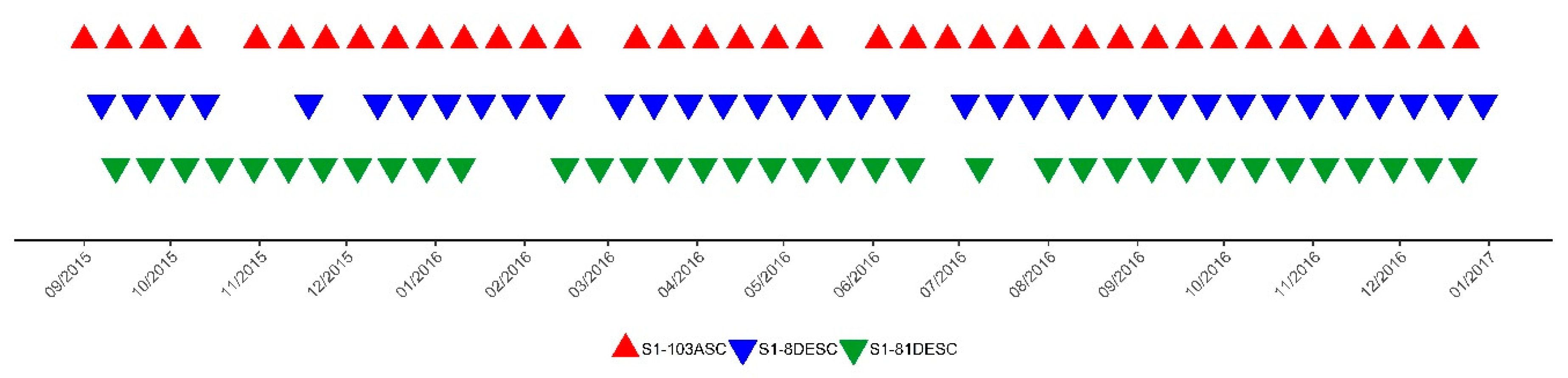
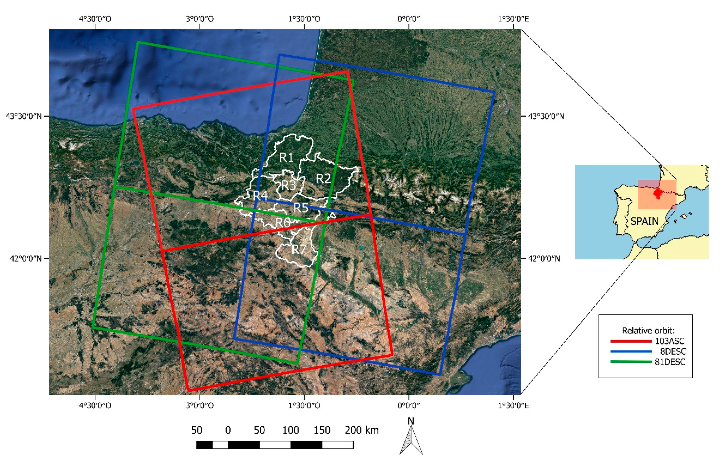
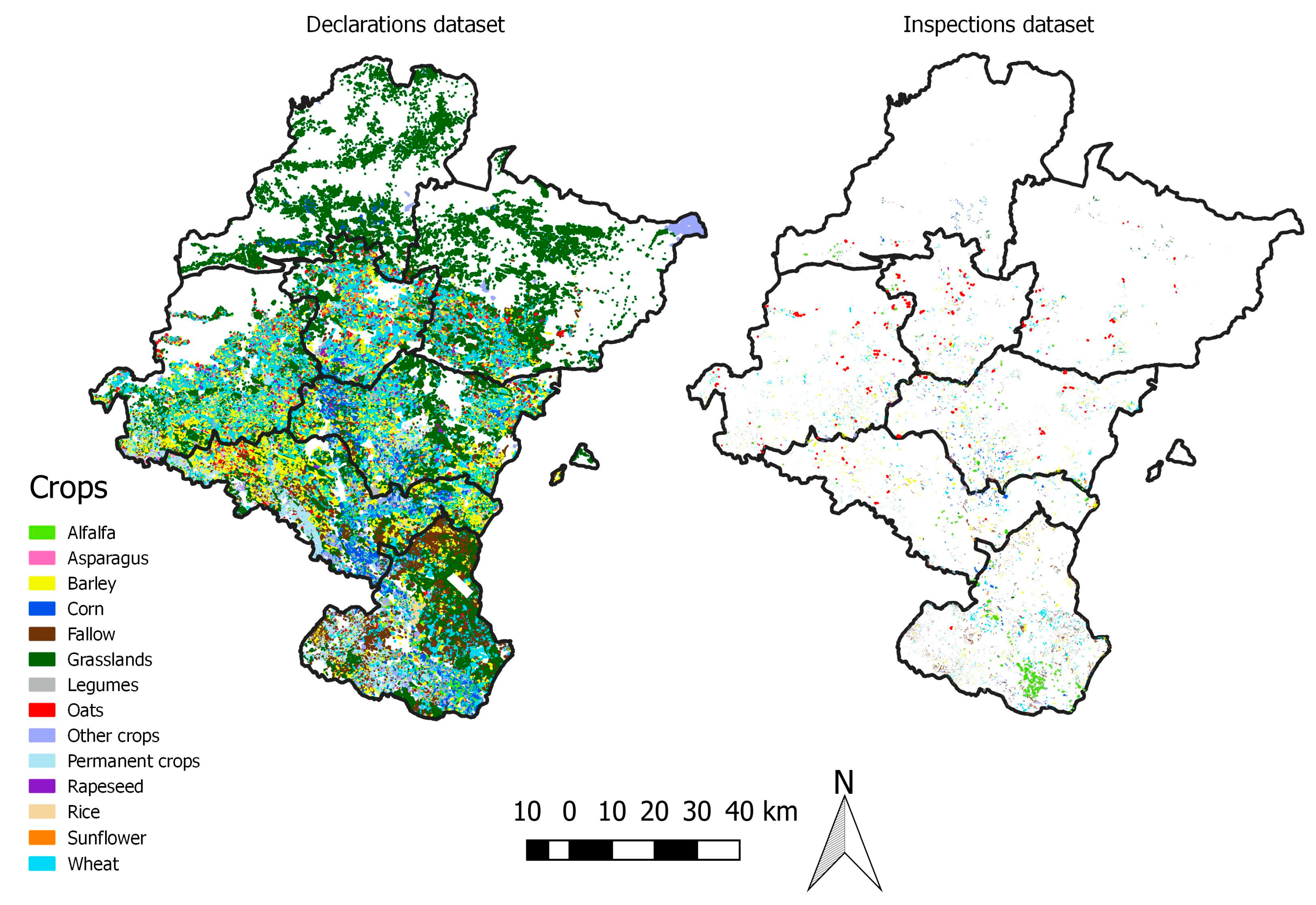
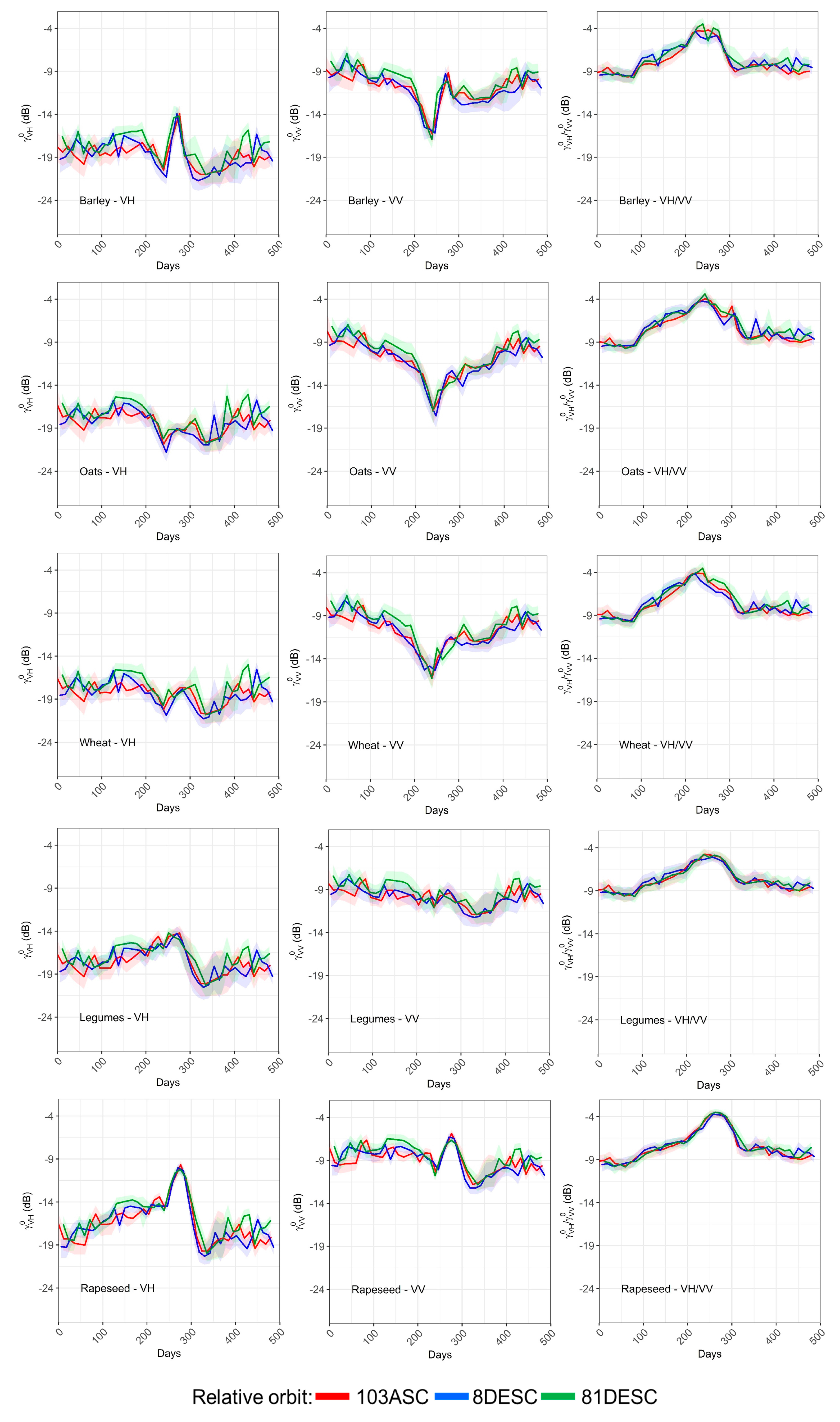
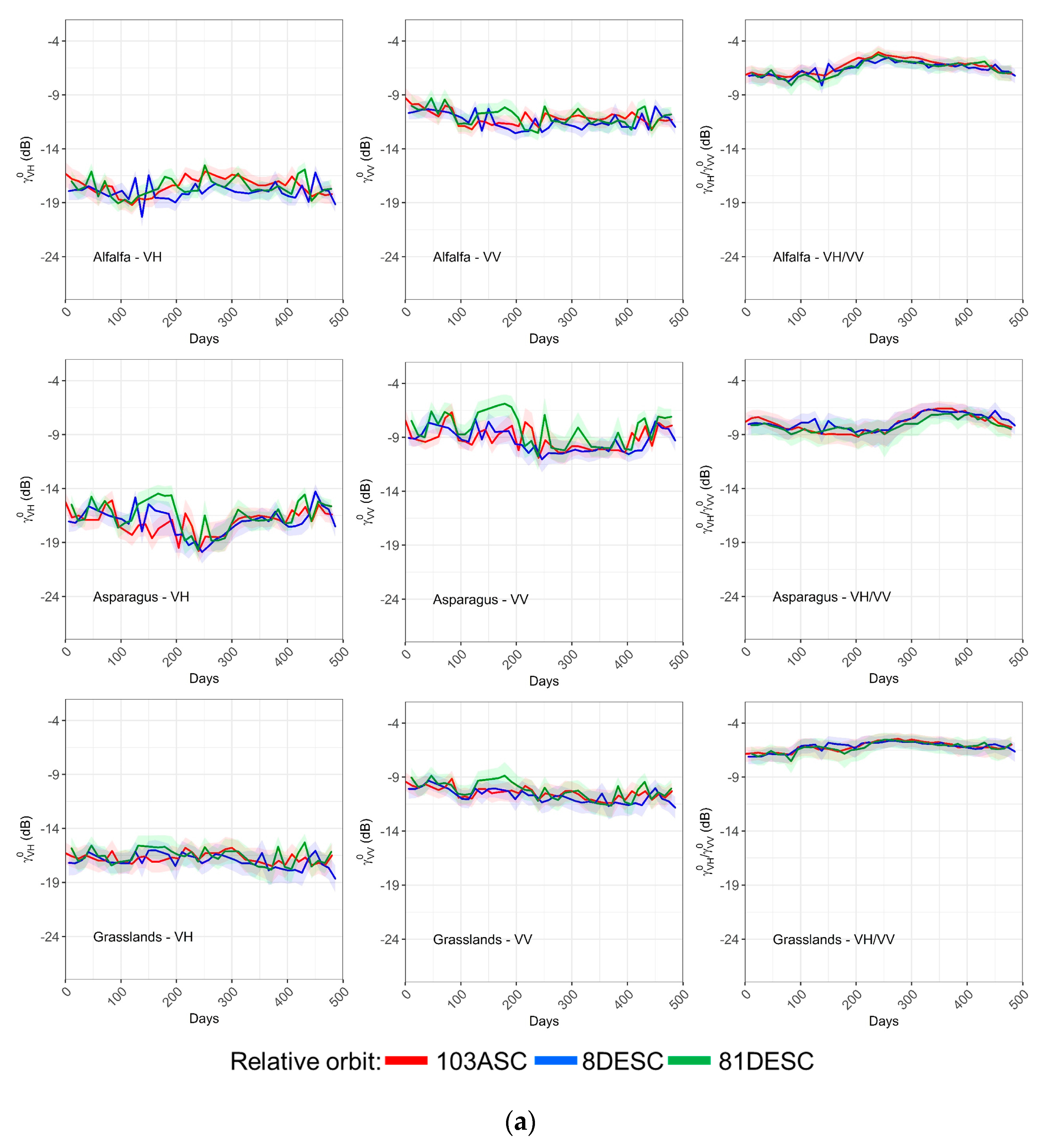
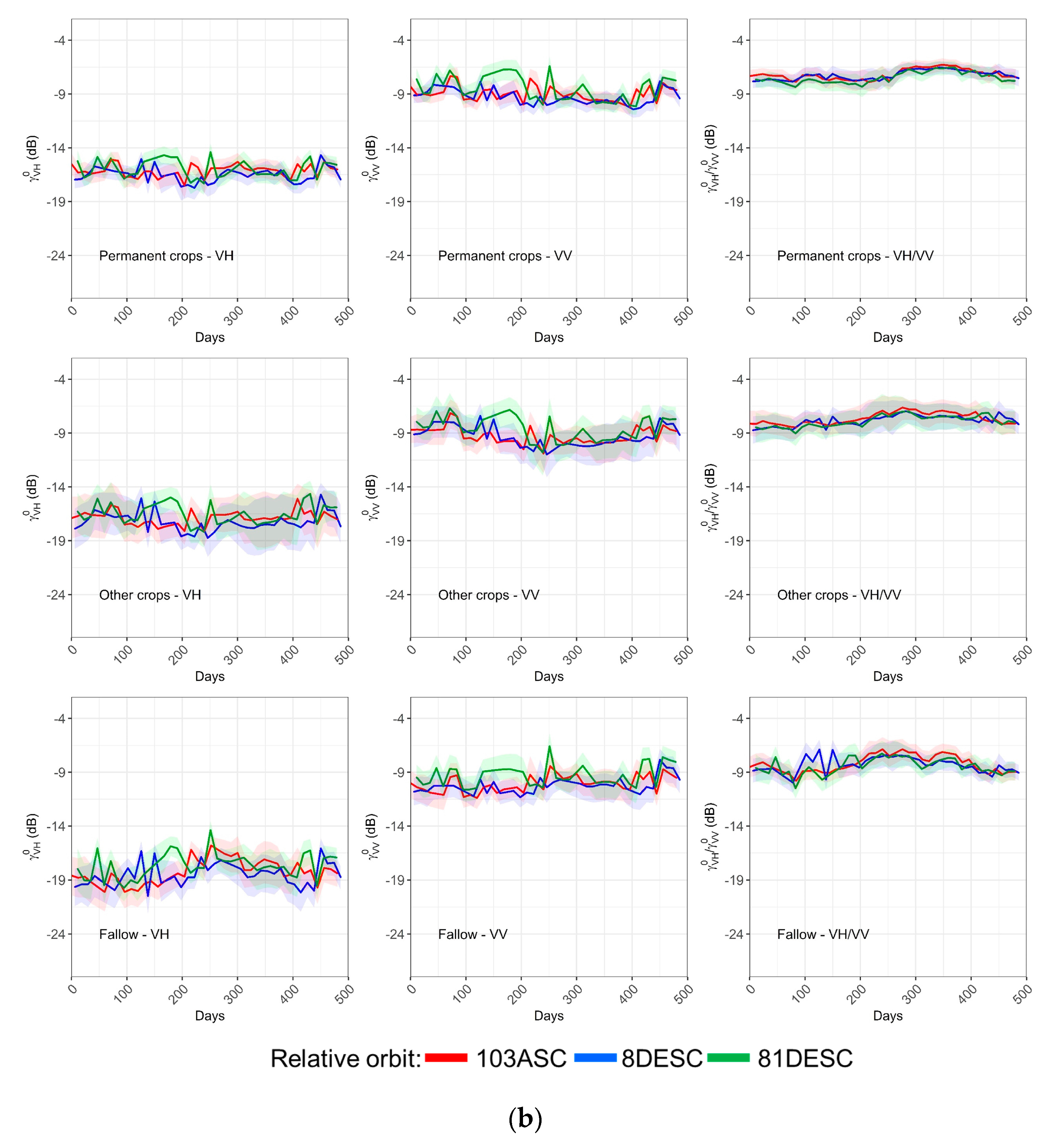
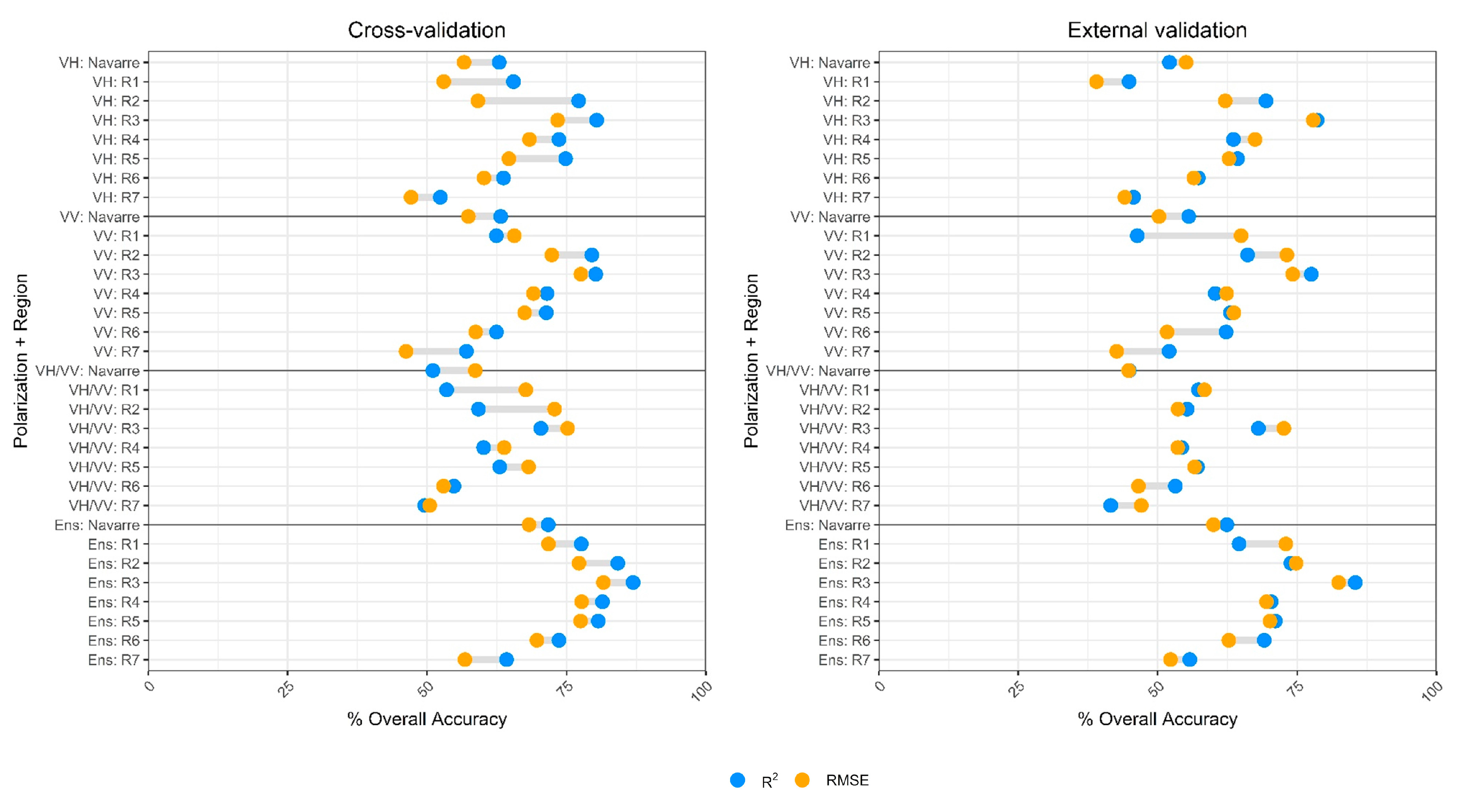
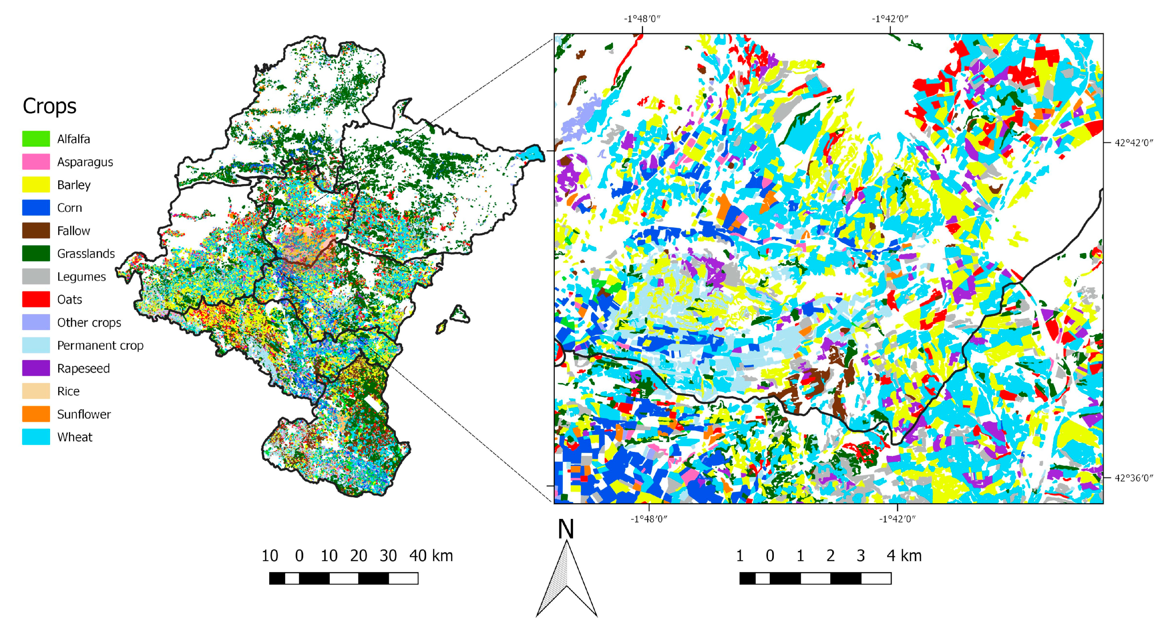
Table 1.
Characteristics of the agricultural regions of Navarre. * Climate classes: O (Oceanic), S (Subalpine), TOM (Transition Oceanic-Mediterranean), M (Mediterranean), CM (Continental-Mediterranean).
Table 1.
Characteristics of the agricultural regions of Navarre. * Climate classes: O (Oceanic), S (Subalpine), TOM (Transition Oceanic-Mediterranean), M (Mediterranean), CM (Continental-Mediterranean).
| Region | Climate | Land Cover (%) | Area (km2) | Elevation (m asl) | |||||
|---|---|---|---|---|---|---|---|---|---|
| Class | Annual Precip. (mm) | Average Temp. (°C) | Rainfed Crops | Irrigated Crops | Forests and Shrubs | Non Productive | |||
| Region 1 | O * | 1700 | 13.8 | 16% | 0% | 81% | 3% | 1903 | 7–1443 |
| Region 2 | S * | 1500 | 8.7 | 14% | 0% | 84% | 2% | 2312 | 225–2428 |
| Region 3 | TOM * | 900 | 12.5 | 47% | 1% | 43% | 9% | 778 | 327–1254 |
| Region 4 | TOM * | 930 | 12.0 | 41% | 2% | 54% | 3% | 1542 | 324–1456 |
| Region 5 | M * | 655 | 12.7 | 44% | 7% | 47% | 2% | 1302 | 304–1260 |
| Region 6 | M * | 350 | 14.0 | 41% | 30% | 25% | 4% | 1226 | 259–652 |
| Region 7 | CM * | 385 | 13.5 | 31% | 33% | 29% | 6% | 1329 | 226–744 |
Table 2.
Ground truth data. Number of agricultural fields and their area in the declarations and inspections datasets for the whole province of Navarre.
Table 2.
Ground truth data. Number of agricultural fields and their area in the declarations and inspections datasets for the whole province of Navarre.
| Crop | Declarations | Inspections | ||||||
|---|---|---|---|---|---|---|---|---|
| Nº of Fields | Area (ha) | Area (%) | Mean Field Area (ha) | Nº of Fields | Area (ha) | Area (%) | Mean Field Area (ha) | |
| Alfalfa | 1747 | 3066 | 1.1% | 1.76 | 397 | 482 | 1.9% | 1.21 |
| Asparagus | 430 | 860 | 0.3% | 2.00 | 61 | 84 | 0.3% | 1.38 |
| Barley | 21,711 | 52,427 | 19.1% | 2.41 | 2705 | 5048 | 20.3% | 1.87 |
| Corn | 3814 | 10,693 | 3.9% | 2.80 | 589 | 1682 | 6.8% | 2.86 |
| Fallow | 11,889 | 23,346 | 8.5% | 1.96 | 3089 | 4785 | 19.2% | 1.55 |
| Grasslands | 25,607 | 81,230 | 29.6% | 3.17 | 512 | 823 | 3.3% | 1.61 |
| Legumes | 3776 | 11,544 | 4.2% | 3.06 | 637 | 1211 | 4.9% | 1.90 |
| Oats | 2969 | 7336 | 2.7% | 2.47 | 268 | 478 | 1.9% | 1.79 |
| Other crops | 3025 | 10,094 | 3.7% | 3.34 | 838 | 1921 | 7.7% | 2.29 |
| Permanent crops | 8329 | 13,342 | 4.9% | 1.60 | 2010 | 2190 | 8.8% | 1.09 |
| Rapeseed | 1250 | 3319 | 1.2% | 2.66 | 226 | 544 | 2.2% | 2.41 |
| Rice | 637 | 1415 | 0.5% | 2.22 | 72 | 125 | 0.5% | 1.73 |
| Sunflower | 799 | 2382 | 0.9% | 2.98 | 102 | 311 | 1.2% | 3.05 |
| Wheat | 20,722 | 53,502 | 19.5% | 2.58 | 2882 | 5216 | 20.9% | 1.81 |
| Total | 106,705 | 274,556 | 100.0% | 2.57 | 14,388 | 24,900 | 100.0% | 1.73 |
Table 3.
Period of time considered for the comparison depending on the crop type.
| Crops | Period of Comparison |
|---|---|
| Barley, legumes, oats, rapeseed and wheat | September 2015 to July 2016 |
| Corn, rice and sunflower | April 2016 to December 2016 |
| Rest of crops | September 2015 to December 2016 |
Table 4.
Mean JM distances for all the pairs of crops for each statistical feature and polarization. The JM distances reported correspond to the average values for the whole period of study.
Table 4.
Mean JM distances for all the pairs of crops for each statistical feature and polarization. The JM distances reported correspond to the average values for the whole period of study.
| Polarization | Max | Min | Mean | Median | SD |
|---|---|---|---|---|---|
| VH | 0.20 | 0.23 | 0.29 | 0.29 | 0.08 |
| VV | 0.17 | 0.23 | 0.29 | 0.29 | 0.06 |
| VH/VV | 0.18 | 0.18 | 0.32 | 0.31 | 0.03 |
Table 5.
F1-score of crops for Ens scheme in Navarre using R2 and RMSE fit metrics.
| Crop Class | F1-Score R2 | F1-Score RMSE |
|---|---|---|
| Alfalfa | 48% | 31% |
| Asparagus | 25% | 22% |
| Barley | 87% | 86% |
| Corn | 78% | 75% |
| Fallow | 70% | 62% |
| Grasslands | 80% | 71% |
| Legumes | 47% | 54% |
| Oats | 42% | 60% |
| Other crops | 12% | 14% |
| Permanent crops | 68% | 58% |
| Rapeseed | 74% | 85% |
| Rice | 85% | 91% |
| Sunflower | 55% | 53% |
| Wheat | 76% | 80% |
Table 6.
Increment (Δ) in crop accuracy (PA, UA and F1-sore) when the stratified regional results are compared to Navarre’s results for Ens scheme (using R2 as the best fit metric).
Table 6.
Increment (Δ) in crop accuracy (PA, UA and F1-sore) when the stratified regional results are compared to Navarre’s results for Ens scheme (using R2 as the best fit metric).
| Crop | Producer’s Accuracy (PA) | User’s Accuracy (UA) | F1-Score | ||||||
|---|---|---|---|---|---|---|---|---|---|
| Navarre | Regions | ΔPA | Navarre | Regions | ΔUA | Navarre | Regions | ΔF1-Score | |
| Alfalfa | 74% | 76% | 2% | 35% | 49% | 14% | 48% | 60% | 12% |
| Asparagus | 60% | 71% | 11% | 16% | 25% | 9% | 25% | 36% | 11% |
| Barley | 90% | 91% | 1% | 85% | 88% | 3% | 87% | 90% | 2% |
| Corn | 75% | 84% | 9% | 81% | 85% | 4% | 78% | 85% | 7% |
| Fallow | 58% | 57% | −2% | 88% | 90% | 2% | 70% | 70% | −1% |
| Grasslands | 71% | 78% | 7% | 92% | 89% | −3% | 80% | 83% | 3% |
| Legumes | 70% | 75% | 6% | 35% | 48% | 13% | 47% | 59% | 12% |
| Oats | 71% | 82% | 11% | 30% | 36% | 6% | 42% | 50% | 8% |
| Other crops | 13% | 19% | 5% | 12% | 25% | 13% | 12% | 21% | 9% |
| Permanent crops | 65% | 72% | 7% | 72% | 72% | 1% | 68% | 72% | 4% |
| Rapeseed | 99% | 97% | −1% | 59% | 70% | 11% | 74% | 82% | 8% |
| Rice | 99% | 99% | 0% | 74% | 85% | 10% | 85% | 91% | 6% |
| Sunflower | 87% | 89% | 1% | 41% | 47% | 6% | 55% | 61% | 6% |
| Wheat | 69% | 80% | 11% | 84% | 85% | 1% | 76% | 82% | 7% |
Table 7.
Confusion matrix of Ens scheme in Navarre (using R2 as the best fit metric). Values are given as a percentage of the total number of fields classified.
Table 7.
Confusion matrix of Ens scheme in Navarre (using R2 as the best fit metric). Values are given as a percentage of the total number of fields classified.

Table 8.
Overall Accuracy for the stratified external validation dataset by field area of Ens scheme (using R2 as the best fit metric).
Table 8.
Overall Accuracy for the stratified external validation dataset by field area of Ens scheme (using R2 as the best fit metric).
| Field Size (ha) | |||
|---|---|---|---|
| <0.5 | 0.5–1 | >1 | |
| Navarre | 51% | 58% | 65% |
| Region 1 | 56% | 66% | 64% |
| Region 2 | 57% | 70% | 75% |
| Region 3 | 75% | 83% | 87% |
| Region 4 | 60% | 65% | 74% |
| Region 5 | 60% | 69% | 72% |
| Region 6 | 62% | 71% | 68% |
| Region 7 | 45% | 51% | 60% |
© 2020 by the authors. Licensee MDPI, Basel, Switzerland. This article is an open access article distributed under the terms and conditions of the Creative Commons Attribution (CC BY) license (http://creativecommons.org/licenses/by/4.0/).
Share and Cite
MDPI and ACS Style
Arias, M.; Campo-Bescós, M.Á.; Álvarez-Mozos, J. Crop Classification Based on Temporal Signatures of Sentinel-1 Observations over Navarre Province, Spain. Remote Sens. 2020, 12, 278. https://0-doi-org.brum.beds.ac.uk/10.3390/rs12020278
AMA Style
Arias M, Campo-Bescós MÁ, Álvarez-Mozos J. Crop Classification Based on Temporal Signatures of Sentinel-1 Observations over Navarre Province, Spain. Remote Sensing. 2020; 12(2):278. https://0-doi-org.brum.beds.ac.uk/10.3390/rs12020278
Chicago/Turabian StyleArias, María, Miguel Ángel Campo-Bescós, and Jesús Álvarez-Mozos. 2020. "Crop Classification Based on Temporal Signatures of Sentinel-1 Observations over Navarre Province, Spain" Remote Sensing 12, no. 2: 278. https://0-doi-org.brum.beds.ac.uk/10.3390/rs12020278
Note that from the first issue of 2016, this journal uses article numbers instead of page numbers. See further details here.