Mapping Landslides on EO Data: Performance of Deep Learning Models vs. Traditional Machine Learning Models


Engineering Geology, Department of Earth Sciences, ETH Zurich, 8092 Zurich, Switzerland
*
Author to whom correspondence should be addressed.
Remote Sens. 2020, 12(3), 346; https://0-doi-org.brum.beds.ac.uk/10.3390/rs12030346
Submission received: 11 December 2019
/
Revised: 9 January 2020
/
Accepted: 16 January 2020
/
Published: 21 January 2020
(This article belongs to the Special Issue Landslide Monitoring, Susceptibility, Hazard Assessment and Prediction with Remotely Sensed Big Data)
Abstract
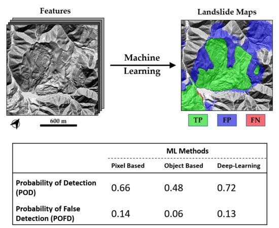
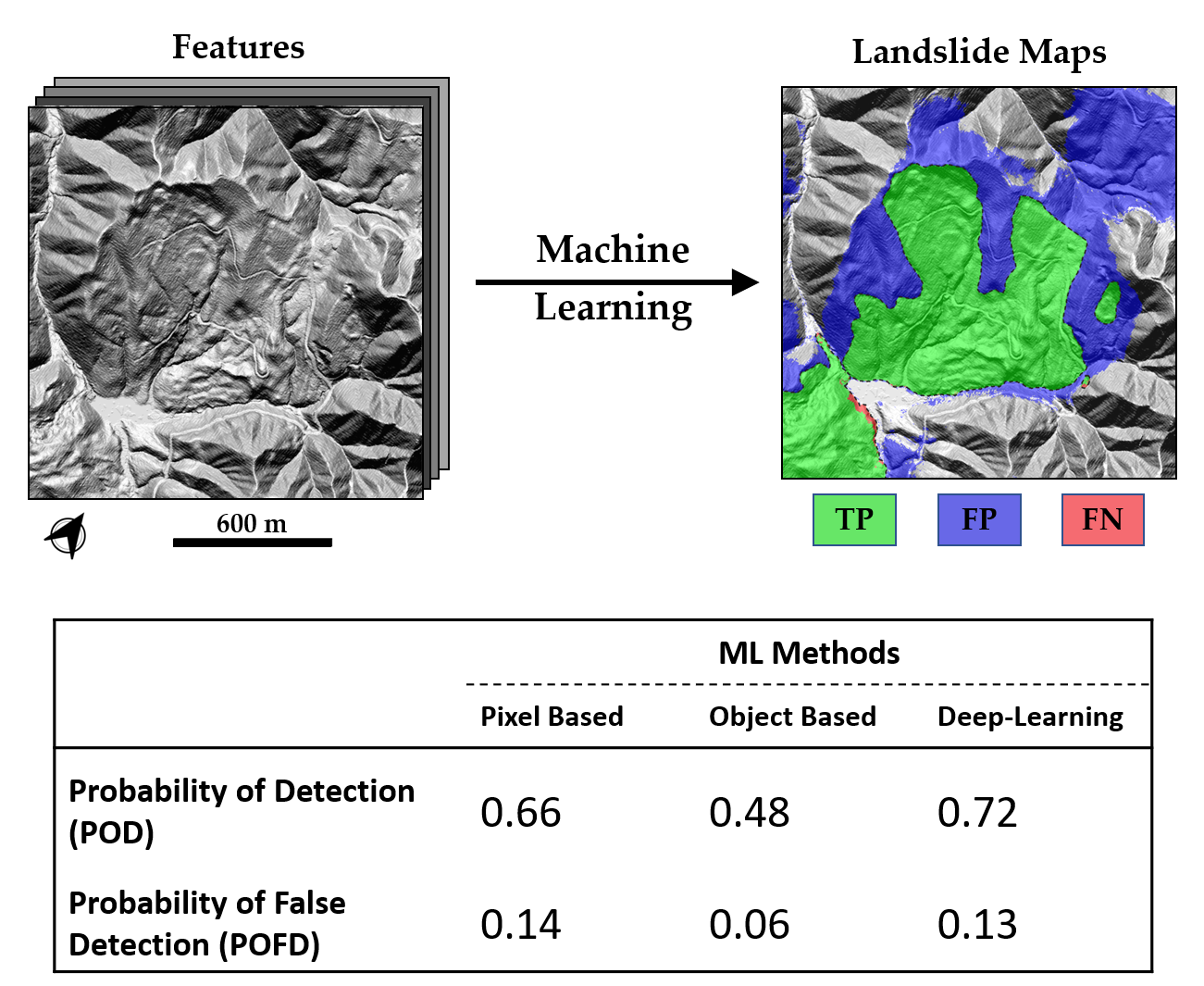
:Mapping landslides using automated methods is a challenging task, which is still largely done using human efforts. Today, the availability of high-resolution EO data products is increasing exponentially, and one of the targets is to exploit this data source for the rapid generation of landslide inventory. Conventional methods like pixel-based and object-based machine learning strategies have been studied extensively in the last decade. In addition, recent advances in CNN (convolutional neural network), a type of deep-learning method, has been widely successful in extracting information from images and have outperformed other conventional learning methods. In the last few years, there have been only a few attempts to adapt CNN for landslide mapping. In this study, we introduce a modified U-Net model for semantic segmentation of landslides at a regional scale from EO data using ResNet34 blocks for feature extraction. We also compare this with conventional pixel-based and object-based methods. The experiment was done in Douglas County, a study area selected in the south of Portland in Oregon, USA, and landslide inventory extracted from SLIDO (Statewide Landslide Information Database of Oregon) was considered as the ground truth. Landslide mapping is an imbalanced learning problem with very limited availability of training data. Our network was trained on a combination of focal Tversky loss and cross-entropy loss functions using augmented image tiles sampled from a selected training area. The deep-learning method was observed to have a better performance than the conventional methods with an MCC (Matthews correlation coefficient) score of and a POD (probability of detection) rate of .
1. Introduction
Landslides are defined as the gravity-driven movement of a mass of rock, debris, or earth down a slope [1]. A sudden slope failure event can be a significant source of economic losses and fatalities when it affects areas of human influence [2]. The World Bank has identified a total land area of 3.7 million square kilometers under risk of landslides, out of which 820 thousand square kilometers are high-risk zones [3]. This affects around 300 million people, which accounts for 5% of the world’s population. Just the non-seismic landslides between 2005 to 2016 are responsible for an underestimated total of 55,997 deaths across the globe [4]. Moreover, the slow-moving unstable slopes hold enough potential to damage or weaken engineering infrastructures like roads, buildings, and dams [5,6]. Occasionally, these instabilities can develop into a rapid-moving catastrophic landslide affecting portions or even entire slopes, often triggered by external factors such as heavy rainfall, earthquakes, volcanic eruptions, and human activities [7]. As the impact of landslides on human lives was proved during last decades, currently its study is an important area in natural hazard research. A lot of work has already been done in studying the mechanics of mass-wasting processes [8] aimed at understanding its relationship with the conditioning factors [9] at identifying hazardous areas and determining the risks involved [10,11].
When a landslide occurs, it changes the topography of the affected area in the form of characteristics surface morphological features, which can be used as a proxy to detect landslide affected slopes [9,12,13]. Maps showing the spatial distribution of past landslides activity and existing slope instabilities are the primary requirement for an effective hazard assessment, risk management, and disaster response. From early days, observing geomorphological features in the field has been the standard procedure to map landslides [14]. Mapping surface features on the field however is a time-consuming process and the scale or location of the phenomena can make it difficult to observe the complete phenomenon at once [13]. After a large catastrophic failure, aerial surveys are often organized for acquiring photographs for stereoscopic aerial photo-interpretation, which complement the field mapping efforts. This provides a synoptic view of large landslides, but conveys no information about the previous state of the ground surface. Today, there is a large constellation of satellites in orbit which systematically acquires and archives Earth Observation (EO) images at high spatial resolution. Visual and semi-automated interpretation of optical satellite images with adequate field validation is currently the most widely used method for making landslide inventories [13,15,16,17]. It is now possible to fetch satellite images from the past for comparative analysis or to study the evolution of an unstable slope. High-resolution Digital Elevation Models (DEM’s) are particularly useful for identifying the morphological features associated with landslides [9,13,18,19,20]. However, most of these observable characteristics markers are post-failure deformation surface features and they do not provide any information about the current state of activity. Depending on the extension of the area of interest and available data, interpretations from the remotely sensed data have important limitations, and require extensive human involvement and include a large degree of subjectivity [21]. This is a major reason that systematic landslide inventory has been compiled for less than 1% of the total slopes present in the land surface [13]. Even if regional landslide catalogs are once mapped, they are often not updated.
The archive of current EO data is increasing exponentially in volume, and the trend is expected to continue in the future due to the planned satellite launches [22,23]. The EO data availability is thus foreseen to rate increase in the order tens of Petabytes per year or more [22], and with such an amount of data it is getting more and more difficult, if not impossible, to analyze all the scenes with manual or semi-automated methods. Hence, the majority of images acquired ends up in archives until it is pulled up for specific investigations. There has been a rapid growth in the application of machine learning across every discipline supported with a complementing increase of digital data and improvement of computing infrastructure. The geoscience community has rapidly adopted machine learning for many applications. There is an ongoing effort towards developing an automated algorithm for mapping of landslides as well. The majority of the work done so far prefers supervised learning approaches, with an assumption that landslides are more likely to occur under conditions similar to those that have caused the past events [12,24,25]. Landslide information of a region, compiled in the past trough manual operation of specialists, can be used to learn patterns from EO data which will further help in automatic identification of landslides in areas which are not yet mapped. In the future, it is foreseen a scenario where it will be possible for a trained algorithm to identify new landslides or even to predict possible locations of slope failure with minimal effort and time.
Geomorphic features resulting from past displacements (for example, scarps, trenches, bulging toes, double ridges) are useful for the identification of landslides. On the other hand, conditioning factors (for example, terrain structure, geology, slope geometry, mean weather conditions, vegetation density, and human-made influences) are the main contributors to the location of landslide formation. Studies that use machine learning algorithms to map landslides from EO data typically have a pre-processing step to derive a broad set of these morphological, hydrological, textural, and spectral features maps. However, many studies have failed to establish a clear distinction between the displacement related features and the conditioning factors. In this work, we collectively refer to displacement related features maps and the conditioning factors maps as “features” or “derived features". These features are used to map “landslides” which we consider to be the areas presenting morphological expressions that can be associated to past and/or recent deformation. Several authors have compiled a brief overview of these features, which are commonly used in the identification of landslides [21,26,27,28] (Table 1). The training process eliminates the requirement of a well-defined physical or numerical model and relies on ad-hoc learning of the relationship between the existing landslide inventory and the derived features. Decision trees (DT) [21,26], artificial neural networks (ANN) [29,30], logistic regressions (LR) [31,32,33], support vector machines (SVM) [29,30,34], discriminant analysis [31,35] are few of the traditional machine learning algorithms which have been popular for mapping landslide and also for mapping landslide susceptibility. Currently, the choice of machine learning methods varies for every study, and there is no consensus for a particular algorithm (Table 2).
Recent advances in Convolutional Neural Networks (CNN), a popular deep-learning architecture, has revolutionized the way to extract information from images. In 2012, Krizhevsky et al. [41] extended the concept of LeNet5 [42] and created the breakthrough AlexNet which won the ImageNet Large Scale Visual Recognition Competition 2012 (ILSVRC). Since then, there has been rapid improvement in learning ability of the CNN architecture to derive complex information from images, which was not previously possible using traditional methods [43,44,45,46]. Deep learning has been aggressively adopted by the remote sensing scientists to extract information from the EO data [23,47]. Bickel et al. [48] have shown significant progress in this direction and were able to detect lunar rockfalls from Lunar Reconnaissance Orbiter Narrow Angle Camera images. Anantrasirichai et al. [49] were able to use CNN for automatic detection of volcanic ground deformation from Sentinel-1 images. In another study, Chen et al. [39] have used CNN to identify areas which have changed in a stack of bi-temporal images, and subsequently used spatio-temporary context analysis to identify landslides. Ghorbanzadeh et al. [29] compared different machine learning methods along with CNN for landslide detection in the higher Himalayas. They observed the results of CNN to be comparable with conventional machine learning methods. Sameen and Pradhan [40] have trained a residual networks (ResNet) on spectral and topographic features to map landslide inventory while comparing different feature merging strategies. However, using semantic segmentation based deep-learning architecture (like U-Net) is expected to outperform a sliding-window CNN for detection of landslides [45].
Today the risk associated with the landslide geohazard is attracting worldwide attention, and management strategies are promoted extensively by large collaborative projects like SafeLand [50], SAFER (Services and Applications For Emergency Response) [7] and BETTER (Big-data Earth observation Technology and Tools Enhancing Research and development) [51]. There is still a requirement for automated rapid mapping of landslides at a regional scale, by learning from the past landslide inventories of the region and its surrounding. In this study, we introduce a new CNN architecture for semantic segmentation of landslides affected regions using information from the high-resolution DEM and optical satellite images. We further compare the performance of this deep-learning approach with conventional machine learning approaches. Section 2 gives an overview of commonly used strategies for mapping landslides using machine learning algorithms, and in Section 3, we introduce the machine learning models used in this study. General information about the selected Douglas County study area and the data sets used for mapping is described in Section 4. A summary of the results obtained from all the applied machine learning approaches are presented in Section 5, which is followed by a short discussion and conclusion in Section 6 and Section 7, respectively.
2. Mapping Landslides on EO with Machine Learning
Training is the most critical step of any machine learning algorithm. Also, training on correctly labeled and large dataset is an important requirement for accurate classification of unseen regions. The training process for landslide mapping starts with splitting the area of training inventory in two separate regions, where one is used to train a machine-learning algorithm, while the other is left to evaluate the performance of the trained model. It is common for the magnitude (area or volume) of landslides to have extremely large variations; hence, the derived features are generated at multiple scales for the success of the classification method [36]. Values sampled from these features using pixel-based (Section 2.1), and object-based (Section 2.2) methods are used as input feature vectors (FVs) for training classical machine learning algorithms. However, in deep-learning methods (Section 2.3), the derived features maps are directly used as an image for training a CNN. A trained model which performs well on the validation area can be further used to map new regions which have not been mapped, provided that the geomorphological and environmental characteristics of the areas are comparable [52].
2.1. Pixel-Based Methods
In the pixel-based methods, the analysis is done by sampling values of derived features over a “fixed-grid” set of points. All the features are treated as a raster, co-registered and re-sampled to a common resolution, which makes it computationally convenient to do a per-pixel analysis. However, pixel-based methods ignore the geometric and contextual information present in the image [21,53,54]. Finding the extent of an existing landslide is difficult using this approach, as a landslide is better represented by a heterogeneous polygon (i.e., a collection of pixels). Detection of landslides activity using image correlation [55,56] and change detection [39,57] are also included in pixel-based methods, but they require a time-series of multi-temporal images.
2.2. Object-Based Methods
In the object-based methods, also known as Object-Based Image Analysis (OBIA) in remote sensing literature, the area of interest is segmented into a group of meaningful homogeneous non-overlapping regions called “super-pixels” or “objects” [58]. This approach assumes that a pixel is very likely to belong to the same class as its neighboring pixels [30]. These objects can be analyzed using spatial, textural, contextual, geometric and spectral characteristics, which are better predictors for identifying landslides [27,38]. A broad set of metrics are calculated for each object and used as an input to the classification algorithms. Most of the reviewed literature using object-based methods use the multiresolution segmentation to extract objects from high-resolution optical images [7,21,58]. But as landslides are hill slope processes, a topography-driven segmentation of the study area can also be meaningful for object-based methods [32,59].
2.3. Deep-Learning Methods
CNN’s have been growing more and more popular in the field of computer vision and image interpretation. These algorithms try to replicate how a human perceives information from an image by learning from a large collection of labeled examples. A trained CNN can extract high-level information from images without the need for explicitly defining specific rules necessary for the task. The availability of large graphics processors with higher memory and faster cores has made it possible to train networks that can learn a significantly larger number of features that are critical in identifying complex patterns in images. The features maps learned in the intermediate layers can also identify past displacement related geomorphic features, which were very difficult to identify using classical satellite image processing methods. Deep-learning is an emerging method in the field of mapping landslides, and to the best of our knowledge, only a few studies have implemented CNN based landslide mapping [29,39,40,60]. Unlike pixel-based and object-based methods, a CNN can directly learn from images, which removes the need for sampling information in the form of numeric FVs.
3. Methodology
Features generated at multiple scales, along with the landslide inventory, are used to train a supervised machine learning model using the three category of methods described in Section 2. The entire process is implemented here in Python programming language with an effort to maintain minimum human input during processing and interpretation. Functions of GDAL [61] and SAGA GIS [62] were used for GIS processing and the machine learning implementation was done using Scikit-learn [63], TensorFlow [64] and Keras [65] libraries.
3.1. Pixel-Based
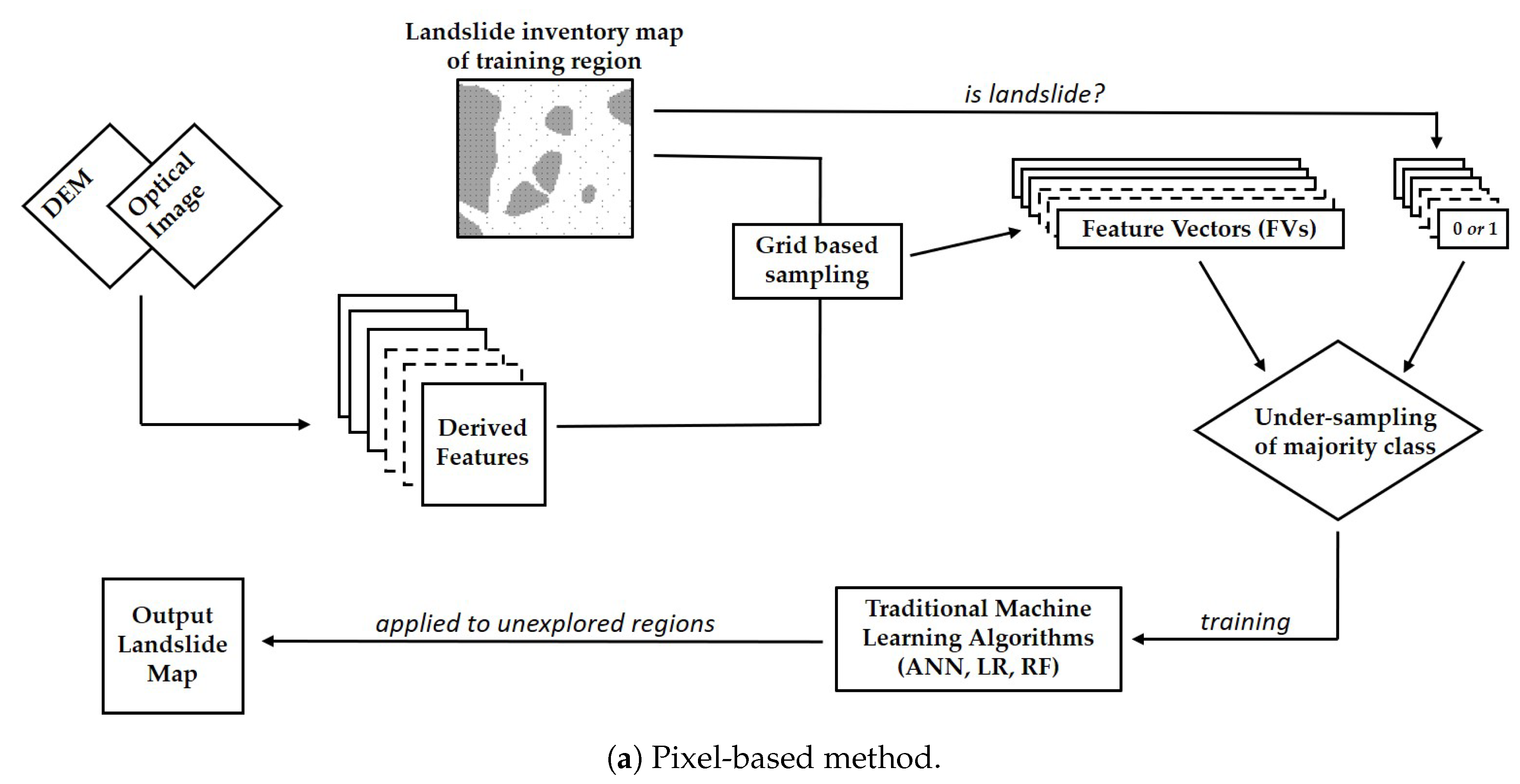
The implementation of pixel-based methods is straightforward. A systematic grid was applied to sample FVs from the conditioning features, which are used as an input for the next steps (Figure 1a). A majority of classification algorithms assume a balanced class distribution [66], and the optimization gets unfavorably biased if the distribution of the training data favors one class over the other. However, landslide inventories are generally biased towards the stable areas. Hence, random under-sampling of the majority class is done to balance the training set. Under-sampling also reduces the number of FVs, which in turn makes the computation faster. Before the final training process, the FVs were standardized by removing the mean and scaling them to unit variance [63].
Three ensemble algorithms, i.e., RF, LR with bagging, and ANN with bagging, were used individually for comparing their performance in the classification of landslide FVs. One hundred DTs were used as base estimators for RF classifier with Gini impurity index as the splitting criteria [67]. Twenty base estimators were used for bagging LR with a regularization strength of 10. Multi-layer perceptron (MLP) with five hidden layers (32, 24, 16, 8, and 16 neurons) and relu activation units was trained with Adam optimizer. The ANN used in this study had 5 of these MLPs as a base estimator for bagging. For clarity, any mention of “LR with bagging” and “ANN with bagging” will be referred to as just “LR” and “ANN” respectively.
3.2. Object-Based
In this method, the first step involves the segmentation of the study area into objects which can be potential candidates for a landslide. A lot of previous works using OBIA for landslide mapping have used high-resolution optical images to segment out the objects. This has worked very well for identifying recent catastrophic events, as there is a distinct visible land cover change associated, for example, loss of vegetation, presence of fresh soil, and deposition of debris. Methods like multiresolution image segmentation and simple linear iterative clustering have been widely used for the segmentation of objects [21,58,68,69].
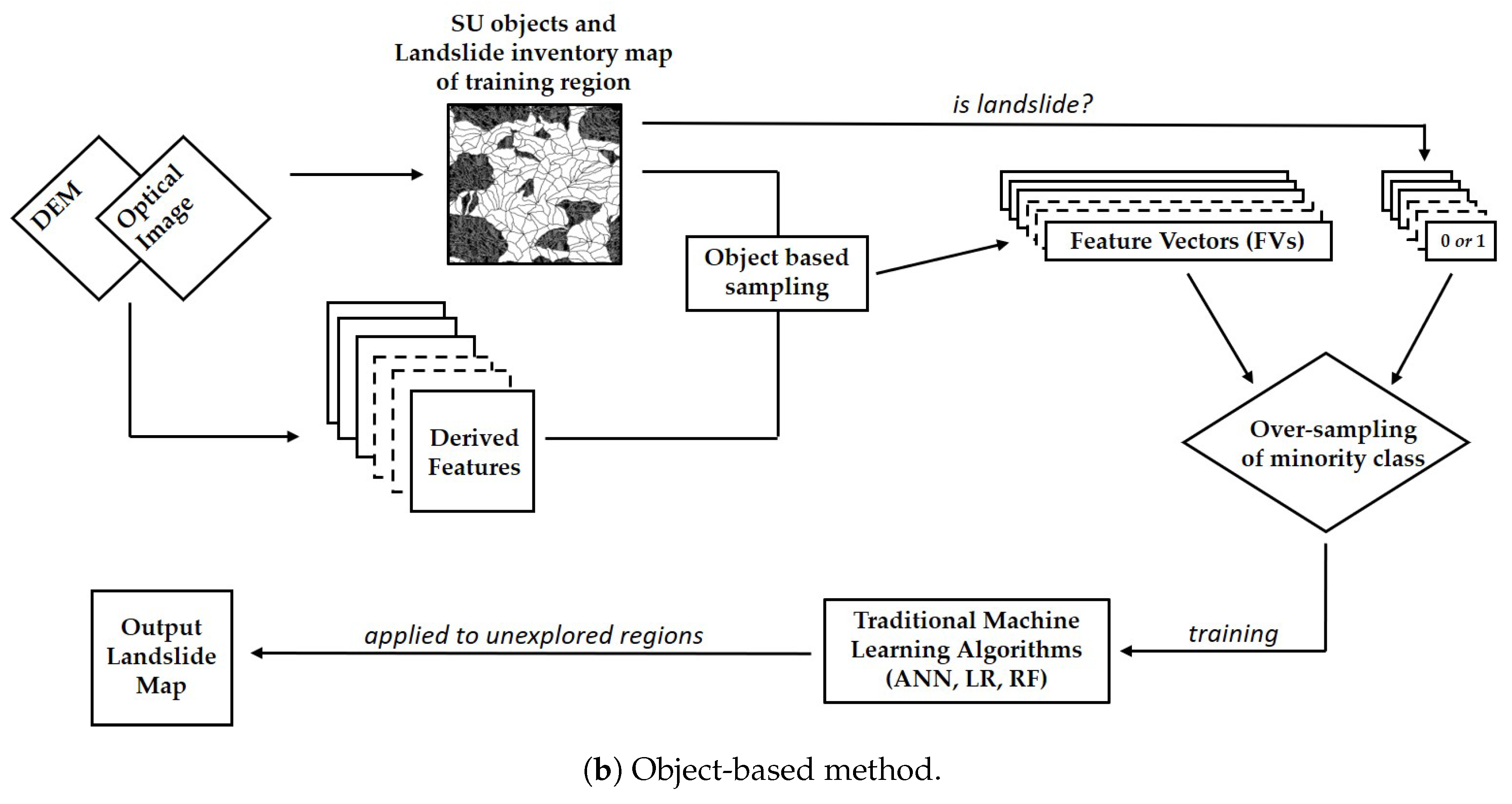
However, when looking for old landslides and/or slow moving landslides, the changes in the land cover are often not very prominent and it gets difficult to distinguish landslide affected slopes from the background in optical images. As the objective of this study is to identify hillslopes which are affected by landslides, it makes sense to segment out the slope facet or “slope units (SUs)” and use it as the object. The use of SUs has been discussed in past works for landslide mapping and susceptibility modeling [12,27,33,59]. Alvioli et al. [33] introduced a method r.slopeunits v1.0 for automated delineation of SUs by iterative subdividing the study area into smaller half basins. In this study, we use this approach to segment out the SUs which are used as objects in the classification process (Figure 1b). SUs which have an 25% overlap with the landslides in the training area were marked as landslides objects. Sampling FVs using object-based methods allow the use of geometric measures, region based statistics and texture metrics to be used in the classification process. The choice and hyper-parameters of the machine learning algorithms remains the same as the pixel-based methods which has already been described in Section 3.1.
3.3. Deep-Learning
Human operators do not rely much on the relationships of the landslide conditioning features. Instead, they typically identify a landslide by visually looking for characteristics surface features in optical images and hillshades of high-resolution DEM [13]. As a CNN is expected to mimic human interpretation of images, a stack of hillshade and optical images will be the primary input to the CNN algorithm. If enough training examples are given, a CNN is expected to learn all the intermediate features required for the classification. As we have limited training examples, we also add a few landslide conditioning features to the input image stack to improve the training of the model.
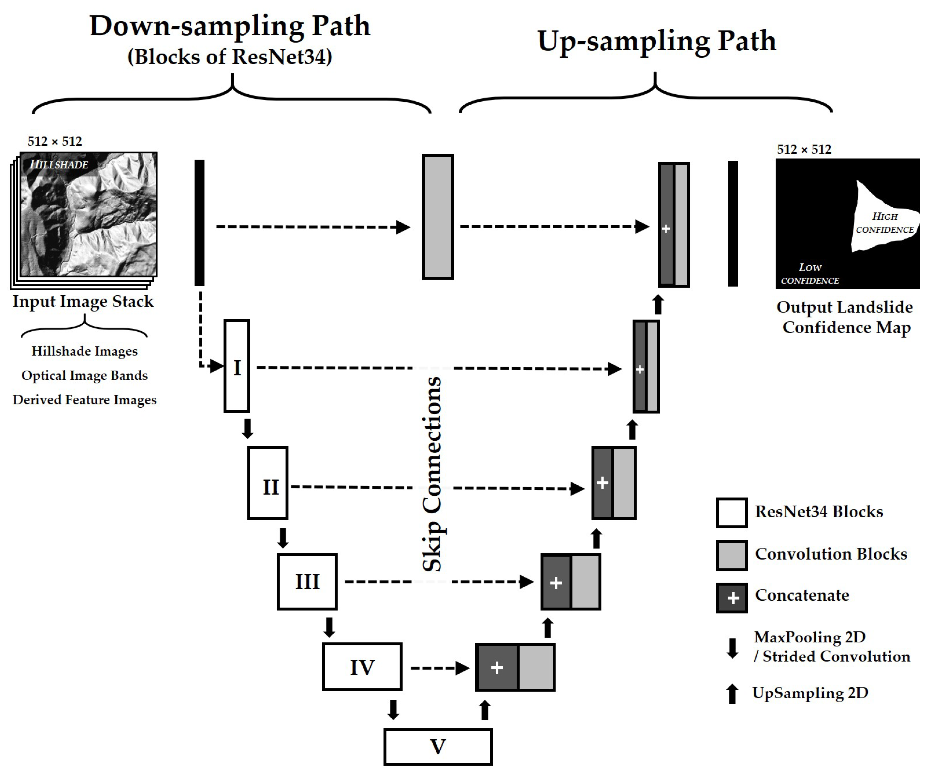
Instead of a standard sliding-window CNN architecture where the down-sampling of the convolutional layer ends in a dense fully-connected layer to give one class label, we propose to use U-net architecture for semantic segmentation of landslide affected regions. U-Net was introduced in 2015 by Ronneberger et al. [45] for segmentation in biomedical images, and has been modified to be used for mapping from satellite images [70,71]. U-Net features the conventional down-sampling path followed by a bottleneck layer and an upsampling path to output a segmentation mask. The skip connections between the down-sampling path and upsampling path recover the spatial information lost during the max pooling operation [72].
ResNet is a very successful CNN architecture for feature extraction in object recognition [44]. We implement a modified U-Net with ResNet34 blocks in the down-sampling path while extracting skip connection at the end of every block for the up-sampling path (Figure 2). The input to the CNN was prepared by generating 512 × 512 tiles of the input image stack and the corresponding landslide image. The current network has more than 33 million trainable parameters, which is difficult to optimize with a small training dataset. Hence, data augmentation techniques have been used to increase the number of training images from the already existing dataset. This was done by generating the input tiles from the training region, an overlap of 50% was used. Also, each of these images were randomly rotated between ±30° and translated by 0% to 10% of the image width during the training process. To handle the class imbalance, images with more than 25% of landslide affected pixels were sampled twice, the second time with a different random augmentation.
Dice similarity coefficient () is a measure of overlap, which has also been widely used for formulating the loss function in semantic segmentation problems [73,74,75,76]. Let G be the ground truth labels and P be the output labels from the network, then is given by:
It can be observed that the score is similar to score, and gives an equal importance to the false positive (FP) and false negative (FN) detections. However, in applications like landslide mapping, FN detections should be minimized. A modified Tversky index (TI), which is a generalization to the DSC, has a coefficient to achieve a better trade-off between precision and recall [75] (Equation (2)). The value of TI can range between 0 and 1, and the CNN is trained by minimizing the loss function defined by Equation (3).
If = , the score simplifies back to score. The value of can be treated as an hyper-parameter of the network and adjusted to increase or decrease the penalty on false negative detections. During the training process, we can decrease the score of well-segmented (and easy to learn) regions to focus the learning on the hard regions with lower score [76,77]. This is done by adding a focusing parameter , to scale down the score where score is high (Equation (4)).
Finally, the modified U-Net with ResNet34 backbone for landslide mapping was trained by minimizing a weighted sum of binary cross-entropy (BCE) loss and . The loss function () is given by:
A small section of training region was kept aside to be used for validation and to track the progress of the training. for the validation set was monitored after every epoch, and the training was stopped when the value of the loss function stopped decreasing for 10 continuous epochs. The weights of every training epoch was saved and the epoch with the best performance in the validation region was finally used for classification.
During the prediction process, we got 512 × 512 tiles as an output from the network with confidence values (between 0 to 1) of finding a landslide. A cut-off threshold of 0.5 is applied to get a binary prediction tile. An overlap-tile strategy was applied for a generating a seamless segmentation map for very large area [45]. From the predicted 512 × 512 segmentation tile, only the center 256 × 256 section was used while stitching the final prediction map to avoid artifacts which are often present at the boundaries.
4. Study Area
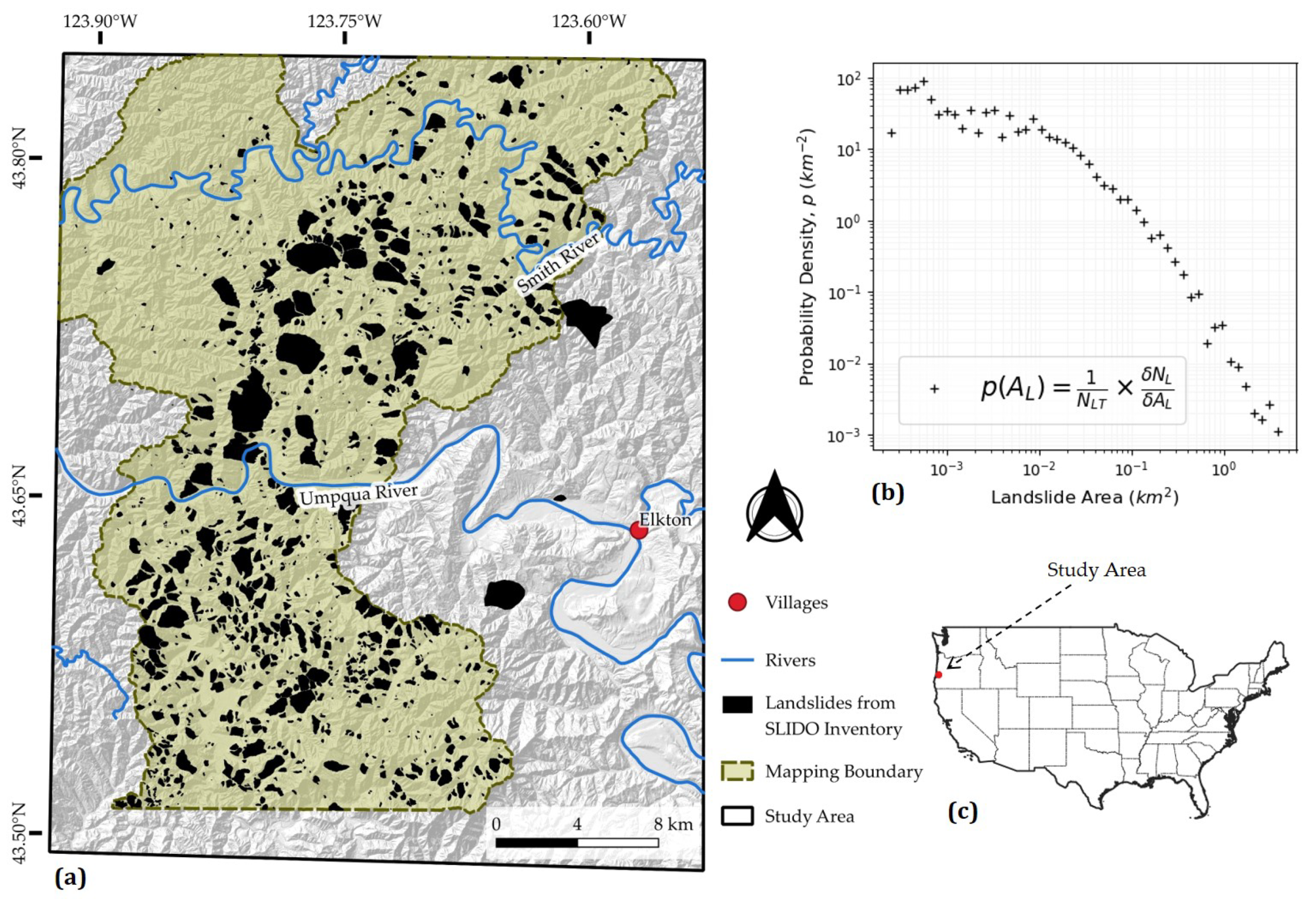
To evaluate the performance of the different ML methods, we selected a study area spread across 1270 km2 between Coos Bay and Eugene in the north western part of Douglas County, Oregon, USA (Figure 3c). It is a mountainous region with elevation ranging from 1 m to 787 m above the sea level. Umpqua and Smith rivers flow westwards into the North Pacific Ocean, which is 22.5 km west of the study area. The geology of the region is mostly sedimentary in origin, and the prominent rock types are turbidite, sandstone and mudstone. Fine-grained and mixed-grained sediments are dominant near the active river channels. The selected study area located in a seismically active region and receives heavy rainfall, which are ideal conditions for triggering landslides [78].
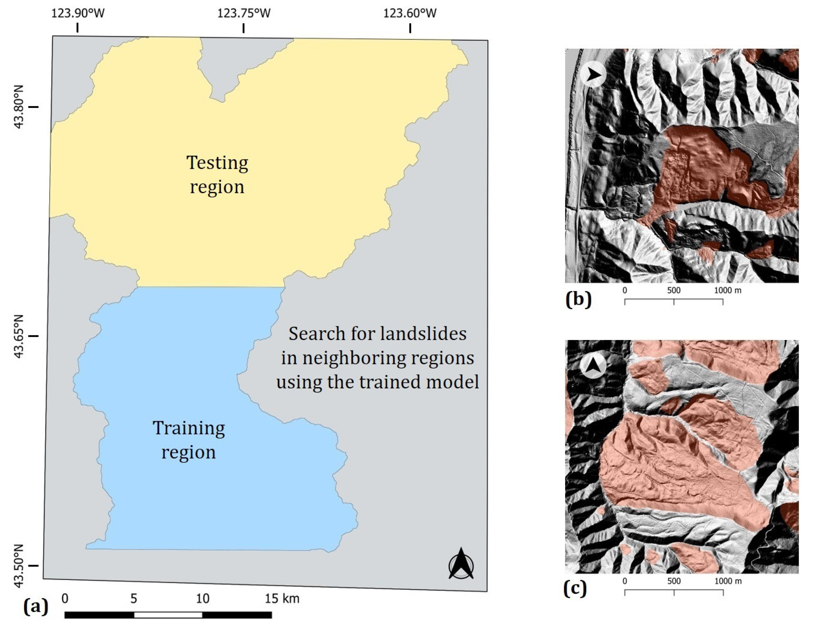
Oregon Department of Geology and Mineral Industries (DOGAMI) maintains a periodically updated Statewide Landslide Information Database for Oregon (SLIDO) [79]. The landslide information in SLIDO has been compiled from multiple published landslide maps due to which the scale of mapping is not consistent across the entire state-wide catalog. A part of our study area was mapped using Lidar images by DOGAMI and Bureau of Land Management (BLM) in 2017 [80] following protocols developed by Burns and Madin [81]. The mapping boundary in Figure 3a shows the extent of the landslide inventory map generated in this study. This inventory has been added to the third release of SLIDO, which we will use for training and testing our machine learning models. We removed rockfalls and debris flows from the inventory as they are morphological very different from the landslides affecting the hill-slopes. All the remaining landslide polygons were rasterized to a resolution of 2 m, and all further analysis was done on this rasterized inventory (Figure 3a). There were 1099 unique landslide features with areas ranging from 252 m2 to 4.63 km2. The landslide magnitude-frequency plot of SLIDO landslide inventory has a rollover at 0.01 km2 (Figure 3b). Figure 4b,c are examples of the surface expression of landslides from the SLIDO inventory on a hillshade layer.
For the training process, landslide inventory has been split into two separate regions (Figure 4a). The landslide inventory from the southern region will be used to train the machine learning models. The held-out northern region, which did not participate in the training process, will be used to validate the performance of the trained model. The trained model can be further applied to expand the surrounding regions which have not been mapped in the 2017 study.
Dataset
For this study, the mapping has been done using a high resolution Lidar DEM and Sentinel-2 cloud-free optical image. Lidar DEM used in this has been made by merging publicly available DOGAMI Lidar Data Quadrangles LDQ-43123-G5 through -G8, LDQ-43123-F5 through -F8, and LDQ-43123-E5 through -E8. Our study area is heavily forested and the bare earth Lidar DEM is particularly useful in observing surface features below the tree cover, which would have been not possible with conventional DEMs [78]. Level-1C Sentinel-2 optical image was downloaded from Copernicus Open Access Hub, and the visible and near-infrared bands at a resolution of 10 m were used in this work. This cloud free image was acquired on 20 October 2018 while the satellite was on a descending track (sensing orbit number 13), and the image footprint covers the entire study area.
The DEM available at a resolution of approximately 1 meter was resampled to 2 m for this study, so that all the surface features from landslides were well preserved while significantly decreasing the data volume and removing artifacts that were present at the original resolution. As a pre-processing step, the input EO data was transformed into a set of characteristics features at multiple resolutions (Table 3). The derived features along with the landslide catalog are converted to raster images, which will be used as an input to the machine learning framework.
5. Results
5.1. Model Assessment Parameters
The trained models for all the three methods are evaluated by individually applying them to the testing region, which was never encountered during the training process. We consider the landslide boundaries from SLIDO inventory to be the ground truth and compare it with the landslide maps generated by the trained models. If a model is able to correctly identify at least 25% of any landslide object in the testing area, we consider it to be detected. To compare the performance of the tested algorithms, a summary of the prediction maps are calculated in the form of a confusion matrix, which includes the true positive, true negative, false positive (FP) and, false negative (FN) values. Based on these values, the accuracy of a model is calculated as follows:
score is the harmonic mean of precision and recall; and like , score also gives equal importance to false positive and false negative detection (Equation (8)). Accuracy and Score works well for performance assessment when working with a balanced dataset, but tends to be misleading in case of class imbalance [82]. On the other hand, Matthews correlation coefficient (MCC) works better to compare on binary classification of imbalanced dataset (Equation (9)). MCC values range between −1 to 1, where a value of 1 represents a perfect classifier, whereas a value of 0 describes a classifier making random guesses.
The probability of detection (POD) and probability of false detection (POFD) are another important set of parameters to be considered while evaluating the performance of the machine learning models [83]:
In the machine learning, POD is also referred to as sensitivity, recall, or true positive rate while POFD is referred to as fall-out or false positive rate. The priority in landslide mapping is to minimize the number of FNs and secondary to limit FPs, which means maximizing POD and minimizing POFD [83]. Higher values of the difference between POD and POFD will indicate a better preforming model. This criteria was also used to select the best weight from all possible weights generated for every epoch in the training process (in Section 3.3).
5.2. Performance Evaluation in the Testing Area
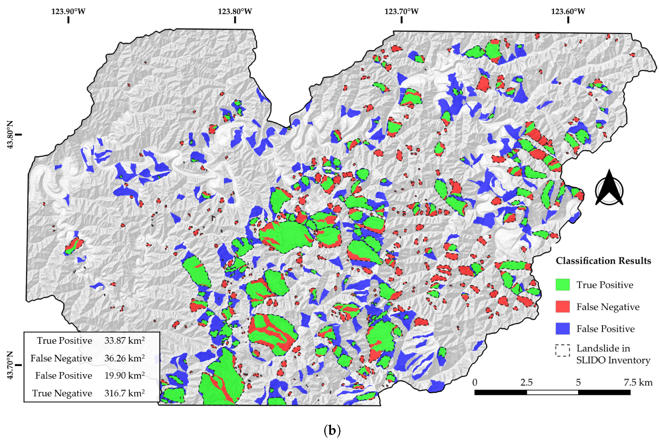
Table 4 and Table 5 summarizes the performance assessment of all tested algorithms. For the pixel-based algorithms, RF and ANN were comparable in detecting the landslides, while LR had the worst performance. All the algorithms showed high false positives, with LR detecting 22.1% of the testing area while RF detected just 12.3% of the testing area. Compared to this, the true positive detection for RF was 8.8% of the testing area and false negative detection was just 4.4% of the total testing area (Figure 5). Post-processing the detection with simple morphological operations could increase the overall classification accuracy. However, we have not considered any post-processing operations in our comparison, but rather focus on the output from the machine learning algorithms. The accuracy values of RF and ANN is above 80%; however, these numbers are misleading as they have been dominated by the true negative detections.
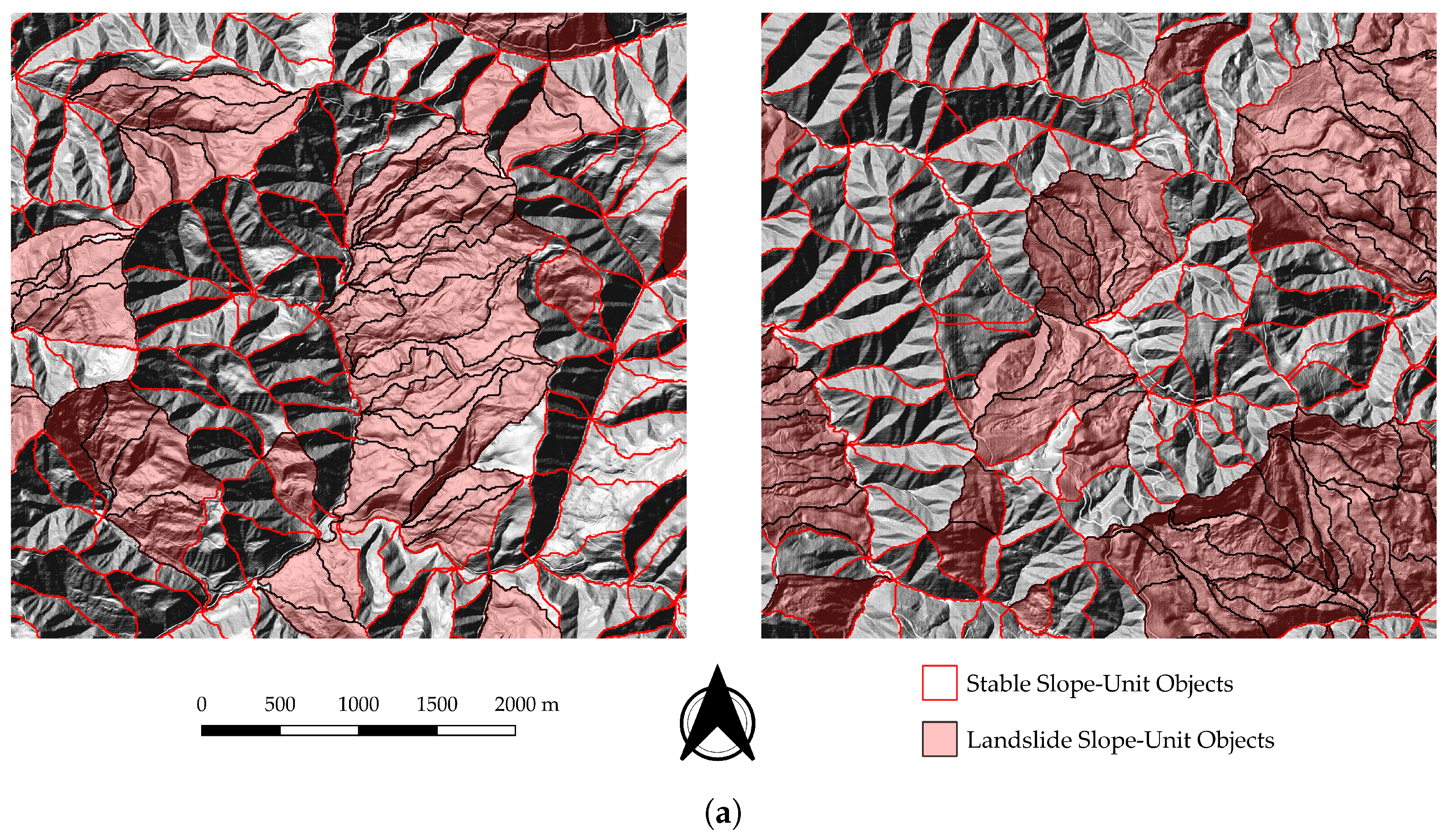
For object-based analysis, the study area was segmented into 10,577 slope units using r.slopeunits v1.0 [33]. The minimum area was 0.1 km2 and the circular variance was 0.1 as the parameter for segmenting the SUs. Figure 6a shows examples of the segmented SUs as an overlay on a hillshade layer. In the testing region, ANN had the best MCC score when compared to LR, RF and all the pixel-based methods. The false positive detection for ANN was 4.9% of the total testing area, while the false negative detection was 8.9% of the total testing area. This method showed the least POFD, but had a significantly low POD.
The modified U-Net with ResNet34 backbone was trained on a stack of hillshade images generated from the DEM at a solar elevation of 45° and an azimuth of 45°, 180°, and 135° along with other features mentioned in Table 3. During the training process with a constant learning rate of , the lowest value achieved for the validation region was 0.475 at the 9th epoch.
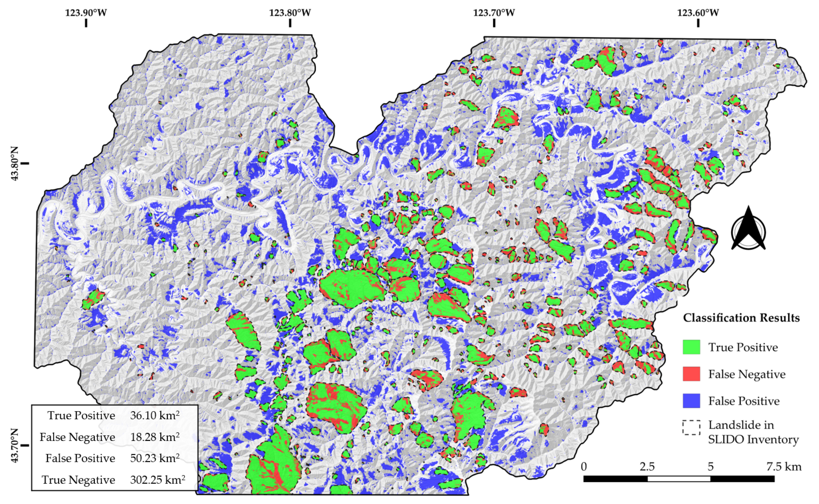
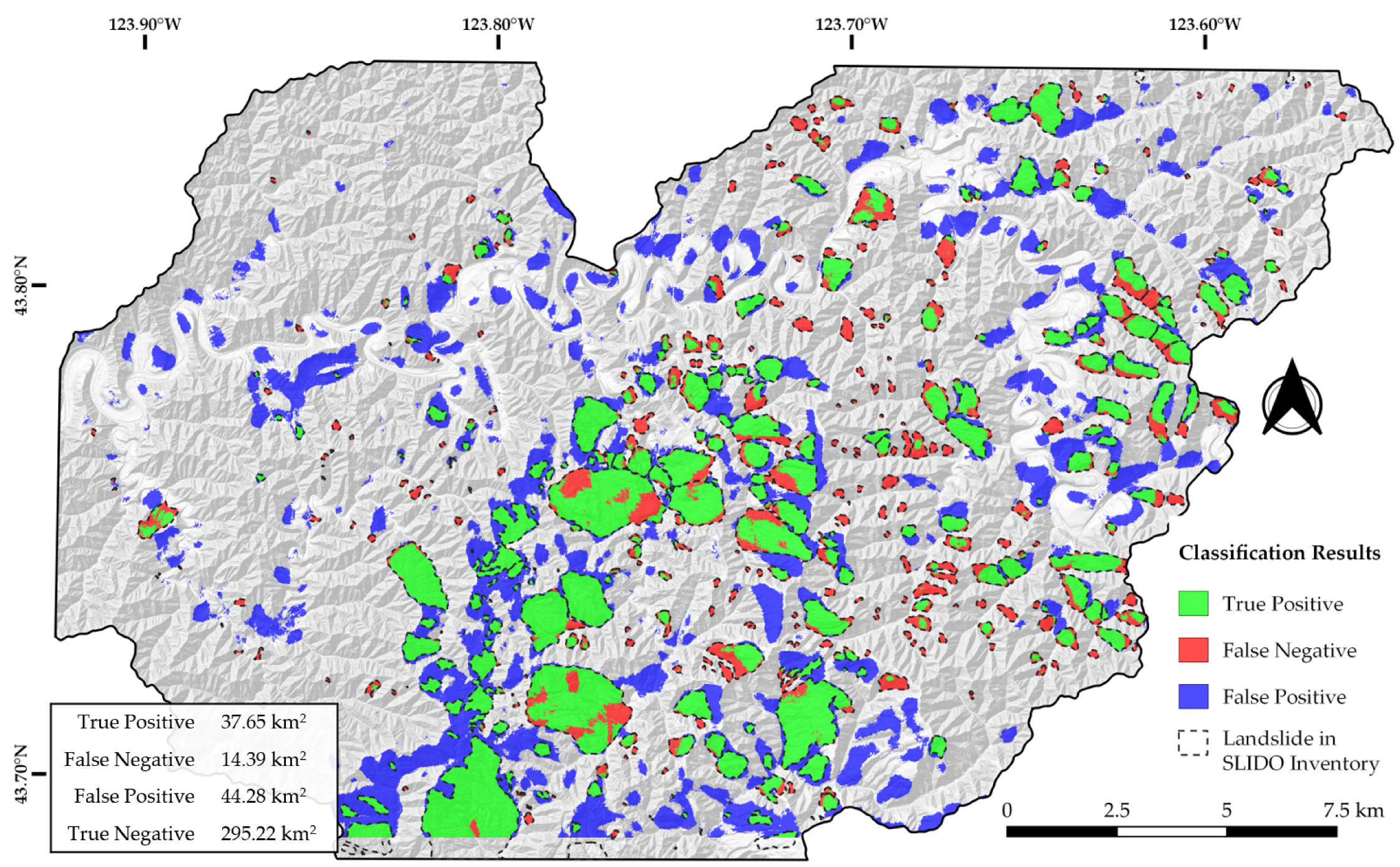
The trained model was applied to the testing region, and the result is shown in Figure 7. This CNN has a better performance when compared to all the previously tested algorithms in terms of MCC value (Table 4 and Table 5). The false positive detection and false negative detection for the CNN was 11.3% and 3.7% of the total testing area respectively. The algorithm missed many small landslides, especially to the east of 123.7°W longitude in Figure 7. Still, the difference of POD and POFD is 0.59 and is higher than the traditional machine learning methods.
6. Discussions
This study supports the observation of Ghorbanzadeh et al. [29] and shows that all the three methods are able to map the landslides in the testing area, with the deep-learning methods performing slightly better than the other two conventional methods. The study area is covered by dense vegetation, and it was difficult to observe landslides from just the optical images. The use of Lidar derived high resolution DEM helped in getting the information of the bare-earth topography, which was critical in mapping the landslides of the region.
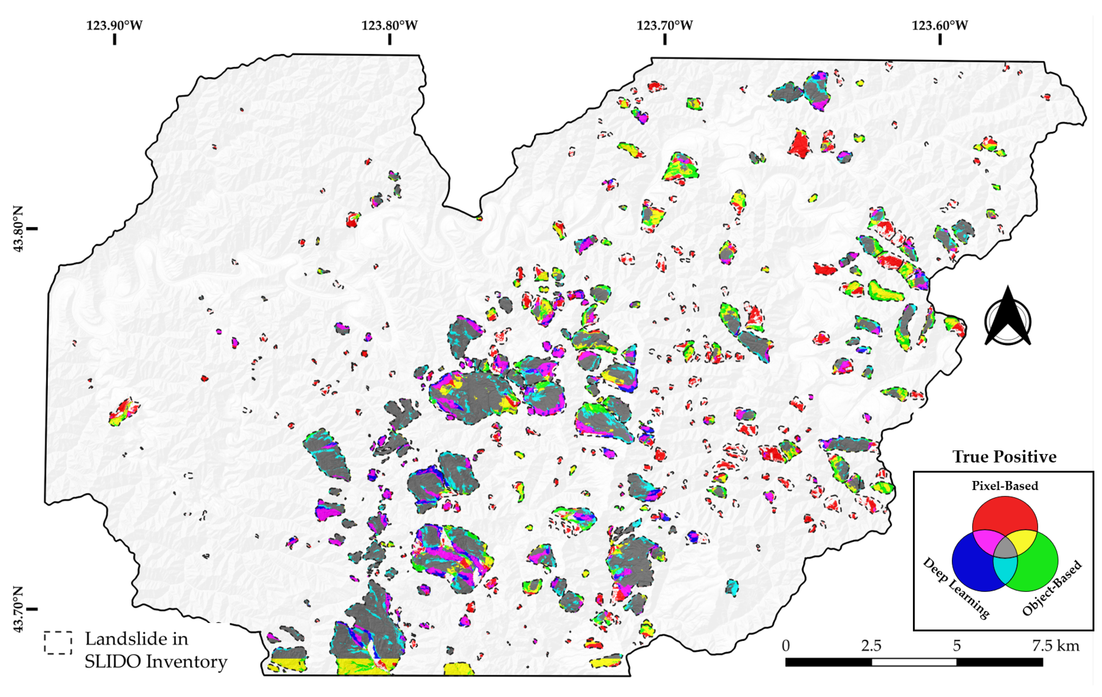
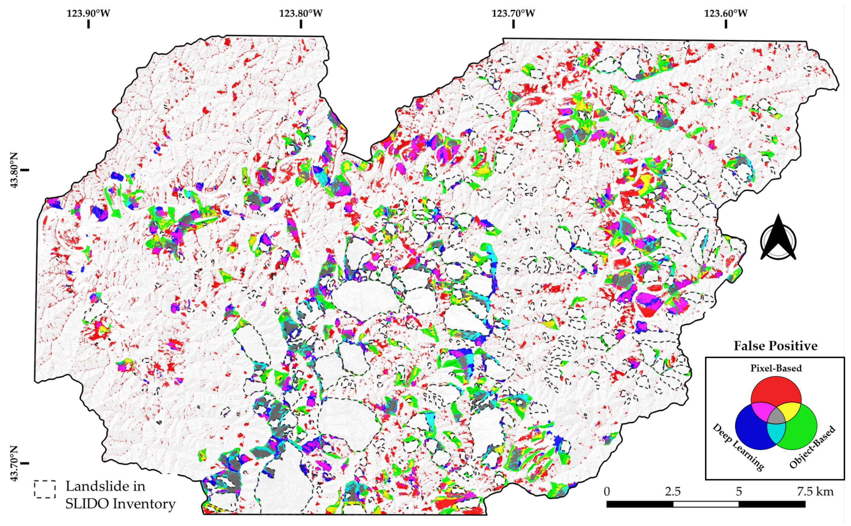
As already defined in Section 5.1, a landslide is considered to be detected only if 25% of its area has been correctly identified. All the three tested methods were able to detect landslides larger than km in the testing region, which is evident by the dominant gray color inside the boundaries of larger landslides in Figure 8. However, correctly detecting the smaller landslides was a problem for all the three methods but the pixel-based method preformed better in detecting them. This can be seen as dominant red color inside the boundaries of smaller landslides in Figure 8. But this does not qualify the pixel-based method to be considered to be a better algorithm as it has a very high POFD (also refer Figure 5 and Table 5). In Figure 9, these false positives of pixel-based method can be observed as scattered red spots all across the testing area. All the methods have difficulties in discriminating individual landslides when they are adjacent and they tend to predict them together as one big landslide area. Because of this the prediction results do not have the correct shape of a standard landslide profile.
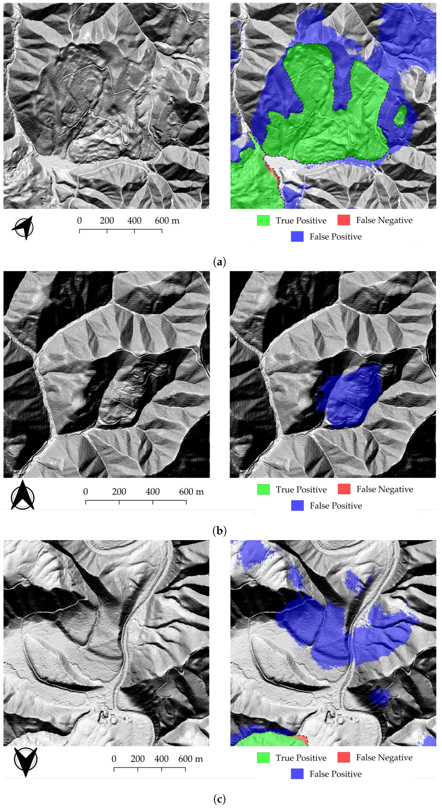
The boundaries of the predicted landslides and landslides in SLIDO database often do not entirely match (See Figure 10a). This is not necessarily a bad result, as human interpretations often have some degree of mismatch while mapping, especially while interpreting the boundaries. The false positives and false negatives areas formed as a consequence of this mismatch contribute in degrading the performance evaluation scores to some extent. On visual inspection, the boundaries of landslides predicted by deep-learning had a close resemblance to a human interpretation of landslides from EO data.
The false positive detections should be taken carefully into account, as they could help us point towards missing information in the landslide inventory used for training. Figure 10b shows once such example of a false positive detection by the deep-learning method in the testing area. Visual analysis show surface features which are comparable to a landslide affected slope, but this information currently missing in the original SLIDO database. These examples show how machine learning methods can be important to update and/or complete existing inventories. However, we also have multiple false positive detections along the Smith River in the north of the testing area, where the surface topography is similar to the example shown in Figure 10c. A possible reason can be the absence of similar surface features in the training region. This example also highlights a very important point, that the training area should have enough variations to cover examples from all possible topographical features which can be present in the mapping area. Similar issues can be reduced by providing more training examples, and/or re-training the network after validation of the results by expert operators.
In the field of hazard management, like landslide mapping, a false alarm has a higher tolerance when compared to a missed alarm [83]. All the tested methods had false negative predictions, which is a cause of concern. This can be controlled by applying a strict threshold to the POFD rates while selecting the best model.
According to the method described in this study (Section 3.3), the prediction of the deep-learning method is tiled and only half of the predicted tile is considered while stitching back the final map. For this reason, the deep-learning methods will not work for prediction near the edge of the EO data. This is strikingly visible in prediction at the bottom regions of testing area (see Figure 7 and Figure 8).
7. Conclusions
The popularity of deep-learning to map landslides from EO images is increasing rapidly [29,40]. Here we approached landslide mapping using CNN as a semantic segmentation task, which was lacking in previous works. This work introduces a U-Net with a ResNet34 feature extraction backbone and compares it with traditional machine learning methods for landslide mapping. We applied our method successfully at a regional scale and show that it outperforms pixel-based and object-based machine learning methods. Similar applications of deep learning based on EO imagery will be very useful in rapid mapping of large areas, which would have been so far a very difficult task to achieve manually. However, we get no indication of the current state of activity on the affected slopes. It would be beneficial to identify the status of activity of landslide affected slopes, which is an important indicator to define landslide hazard potential. Also, post-processing the results with contextual information will help to decrease false positive predictions. Studies for semantic segmentation in other fields have used successfully used conditional random fields to post-process their segmentation results [84], and should also be in future explored for landslide mapping context.
Author Contributions
Conceived the foundation, A.M.; Designed the methods, N.P.; Preformed the experiments, N.P.; Interpretation of results, A.M. and N.P.; Supervision, A.M. and S.L.; Writing the original draft, N.P.; All the co-authors revised the manuscript; Funding Acquisition, A.M. and S.L. All authors have read and agreed to the published version of the manuscript.
Funding
This research was done in the framework of BETTER project (European Union’s Horizon 2020 Research and Innovation Program under grant agreement No. 776280).
Acknowledgments
The authors thank Jordan Aaron from Department of Earth Sciences, ETH Zurich for providing information on the study area. They would also like to thank the two anonymous reviewers for their valuable comments. The use of landslide inventory and lidar images of Oregon, USA was critical for this work and were obtained from repositories maintained by USGS/DOGAMI.
Conflicts of Interest
The authors declare no conflict of interest.
References
- Cruden, D.M. A simple definition of a landslide. Bull. Eng. Geol. Environ. 1991, 43, 27–29. [Google Scholar] [CrossRef]
- Turner, A.K. Social and environmental impacts of landslides. Innov. Infrastruct. Solut. 2018, 3, 70. [Google Scholar] [CrossRef]
- Dilley, M.; Chen, R.S.; Deichmann, U.; Lerner-Lam, A.; Arnold, M.; Agwe, J.; Buys, P.; Kjekstad, O.; Lyon, B.; Yetman, G. Natural Disaster Hotspots: A Global Risk Analysis (English); World Bank: Washington, DC, USA, 2005; pp. 1–132. [Google Scholar]
- Froude, M.J.; Petley, D.N. Global fatal landslide occurrence from 2004 to 2016. Hazards Earth Syst. Sci. 2018, 18, 2161–2181. [Google Scholar] [CrossRef] [Green Version]
- Cooper, A.H. The classification, recording, databasing and use of information about building damage caused by subsidence and landslides. Q. J. Eng. Geol. Hydrogeol. 2008, 41, 409–424. [Google Scholar] [CrossRef] [Green Version]
- Tomás, R.; Abellán, A.; Cano, M.; Riquelme, A.; Tenza-Abril, A.J.; Baeza-Brotons, F.; Saval, J.M.; Jaboyedoff, M. A multidisciplinary approach for the investigation of a rock spreading on an urban slope. Landslides 2018, 15, 199–217. [Google Scholar] [CrossRef] [Green Version]
- Casagli, N.; Cigna, F.; Bianchini, S.; Hölbling, D.; Füreder, P.; Righini, G.; Del Conte, S.; Friedl, B.; Schneiderbauer, S.; Iasio, C.; et al. Landslide mapping and monitoring by using radar and optical remote sensing: Examples from the EC-FP7 project SAFER. Remote Sens. Appl. Soc. Environ. 2016, 4, 92–108. [Google Scholar] [CrossRef] [Green Version]
- Stead, D.; Wolter, A. A critical review of rock slope failure mechanisms: The importance of structural geology. J. Struct. Geol. 2015, 74, 1–23. [Google Scholar] [CrossRef]
- Pike, R.J. The geometric signature: Quantifying landslide-terrain types from digital elevation models. Math. Geol. 1988, 20, 491–511. [Google Scholar] [CrossRef]
- Soeters, R.; van Westen, C.J. Slope instability recognition, analysis and zonation. In Landslides Investigation and Mitigation (Transportation Research Board, National Research Council, Special Report 247); Turner, A.K., Schuster, R.L., Eds.; National Academy Press: Washington, DC, USA, 1996; pp. 129–177. [Google Scholar]
- Van Westen, C.J.; Castellanos, E.; Kuriakose, S.L. Spatial data for landslide susceptibility, hazard, and vulnerability assessment: An overview. Eng. Geol. 2008, 102, 112–131. [Google Scholar] [CrossRef]
- Guzzetti, F.; Carrara, A.; Cardinali, M.; Reichenbach, P. Landslide hazard evaluation: A review of current techniques and their application in a multi-scale study, Central Italy. Geomorphology 1999, 31, 181–216. [Google Scholar] [CrossRef]
- Guzzetti, F.; Mondini, A.C.; Cardinali, M.; Fiorucci, F.; Santangelo, M.; Chang, K.T. Landslide inventory maps: New tools for an old problem. Earth-Sci. Rev. 2012, 112, 42–66. [Google Scholar] [CrossRef] [Green Version]
- Brunsden, D. Landslide types, mechanisms, recognition, identification. In Landslides in the South Wales Coalfield: Proceedings, Symposium, Polytechnic of Wales—1st to 3rd April, 1985; Morgan, C.S., Ed.; Polytechnic of Wales: Cardiff, UK, 1985; pp. 19–28. [Google Scholar]
- Crosta, G.B.; Frattini, P.; Agliardi, F. Deep seated gravitational slope deformations in the European Alps. Tectonophysics 2013, 605, 13–33. [Google Scholar] [CrossRef]
- Roback, K.; Clark, M.K.; West, A.J.; Zekkos, D.; Li, G.; Gallen, S.F.; Chamlagain, D.; Godt, J.W. The size, distribution, and mobility of landslides caused by the 2015 Mw7.8 Gorkha earthquake, Nepal. Geomorphology 2018, 301, 121–138. [Google Scholar] [CrossRef]
- Sauchyn, D.J.; Trench, N.R. Landsat applied to landslide mapping. Photogramm. Eng. Remote Sens. 1978, 44, 735–741. [Google Scholar]
- Leshchinsky, B.A.; Olsen, M.J.; Tanyu, B.F. Contour Connection Method for automated identification and classification of landslide deposits. Comput. Geosci. 2015, 74, 27–38. [Google Scholar] [CrossRef]
- Derron, M.H.; Jaboyedoff, M. LIDAR and DEM techniques for landslides monitoring and characterization. Nat. Hazards Earth Syst. Sci. 2010, 10, 1877–1879. [Google Scholar] [CrossRef]
- Jaboyedoff, M.; Oppikofer, T.; Abellán, A.; Derron, M.H.; Loye, A.; Metzger, R.; Pedrazzini, A. Use of LIDAR in landslide investigations: A review. Nat. Hazards 2012, 61, 5–28. [Google Scholar] [CrossRef] [Green Version]
- Stumpf, A.; Kerle, N. Object-oriented mapping of landslides using Random Forests. Remote Sens. Environ. 2011, 115, 2564–2577. [Google Scholar] [CrossRef]
- Molch, K.; Unterstein, R. DLR—Earth Observation Center—60 Petabytes for the German Satellite Data Archive D-SDA. 2018. Available online: https://www.dlr.de/eoc/en/desktopdefault.aspx/tabid-12632/22039_read-51751 (accessed on 17 December 2018).
- Zhu, X.X.; Tuia, D.; Mou, L.; Xia, G.S.; Zhang, L.; Xu, F.; Fraundorfer, F. Deep Learning in Remote Sensing: A Comprehensive Review and List of Resources. IEEE Geosci. Remote Sens. Mag. 2017, 5, 8–36. [Google Scholar] [CrossRef] [Green Version]
- Huang, F.; Yin, K.; He, T.; Zhou, C.; Zhang, J. Influencing factor analysis and displacement prediction in reservoir landslides—A case study of Three Gorges Reservoir (China). Tehnički Vjesnik 2016, 23, 617–626. [Google Scholar] [CrossRef] [Green Version]
- Varnes, D. Landslide hazard zonation: A review of principles and practice. Nat. Hazards 1984, 3, 61. [Google Scholar] [CrossRef]
- Micheletti, N.; Foresti, L.; Robert, S.; Leuenberger, M.; Pedrazzini, A.; Jaboyedoff, M.; Kanevski, M. Machine Learning Feature Selection Methods for Landslide Susceptibility Mapping. Math. Geosci. 2014, 46, 33–57. [Google Scholar] [CrossRef] [Green Version]
- Reichenbach, P.; Rossi, M.; Malamud, B.D.; Mihir, M.; Guzzetti, F. A review of statistically-based landslide susceptibility models. Earth-Sci. Rev. 2018, 180, 60–91. [Google Scholar] [CrossRef]
- Agliardi, F.; Crosta, G.; Zanchi, A. Structural constraints on deep-seated slope deformation kinematics. Eng. Geol. 2001, 59, 83–102. [Google Scholar] [CrossRef]
- Ghorbanzadeh, O.; Blaschke, T.; Gholamnia, K.; Meena, S.R.; Tiede, D.; Aryal, J. Evaluation of different machine learning methods and deep-learning convolutional neural networks for landslide detection. Remote Sens. 2019, 11, 196. [Google Scholar] [CrossRef] [Green Version]
- Moosavi, V.; Talebi, A.; Shirmohammadi, B. Producing a landslide inventory map using pixel-based and object-oriented approaches optimized by Taguchi method. Geomorphology 2014, 204, 646–656. [Google Scholar] [CrossRef]
- Mondini, A.C.; Guzzetti, F.; Reichenbach, P.; Rossi, M.; Cardinali, M.; Ardizzone, F. Semi-automatic recognition and mapping of rainfall induced shallow landslides using optical satellite images. Remote Sens. Environ. 2011, 115, 1743–1757. [Google Scholar] [CrossRef]
- Tanyas, H.; Rossi, M.; Alvioli, M.; van Westen, C.J.; Marchesini, I. A global slope unit-based method for the near real-time prediction of earthquake-induced landslides. Geomorphology 2019, 327, 126–146. [Google Scholar] [CrossRef]
- Alvioli, M.; Marchesini, I.; Reichenbach, P.; Rossi, M.; Ardizzone, F.; Fiorucci, F.; Guzzetti, F. Automatic delineation of geomorphological slope units with r.slopeunits v1.0 and their optimization for landslide susceptibility modeling. Geosci. Model Dev. 2016, 9, 3975–3991. [Google Scholar] [CrossRef] [Green Version]
- Huang, Y.; Zhao, L. Review on landslide susceptibility mapping using support vector machines. Catena 2018, 165, 520–529. [Google Scholar] [CrossRef]
- Goetz, J.N.; Cabrera, R.; Brenning, A.; Heiss, G.; Leopold, P. Modelling Landslide Susceptibility for a Large Geographical Area Using Weights of Evidence in Lower Austria. In Engineering Geology for Society and Territory; Springer International Publishing: Cham, Switzerland, 2015; Volume 2, pp. 927–930. [Google Scholar] [CrossRef]
- Martha, T.R.; Kerle, N.; Van Westen, C.J.; Jetten, V.; Kumar, K.V. Segment optimization and data-driven thresholding for knowledge-based landslide detection by object-based image analysis. IEEE Trans. Geosci. Remote Sens. 2011, 49, 4928–4943. [Google Scholar] [CrossRef]
- Calvello, M.; Peduto, D.; Arena, L. Combined use of statistical and DInSAR data analyses to define the state of activity of slow-moving landslides. Landslides 2017, 14, 473–489. [Google Scholar] [CrossRef]
- Keyport, R.N.; Oommen, T.; Martha, T.R.; Sajinkumar, K.S.; Gierke, J.S. A comparative analysis of pixel- and object-based detection of landslides from very high-resolution images. Int. J. Appl. Earth Obs. Geoinf. 2018, 64, 1–11. [Google Scholar] [CrossRef]
- Chen, Z.; Zhang, Y.; Ouyang, C.; Zhang, F.; Ma, J. Automated landslides detection for mountain cities using multi-temporal remote sensing imagery. Sensors 2018, 18, 821. [Google Scholar] [CrossRef] [Green Version]
- Sameen, M.I.; Pradhan, B. Landslide Detection Using Residual Networks and the Fusion of Spectral and Topographic Information. IEEE Access 2019, 7, 114363–114373. [Google Scholar] [CrossRef]
- Krizhevsky, A.; Sutskever, I.; Hinton, G.E. ImageNet Classification with Deep Convolutional Neural Networks. In Proceedings of the 25th International Conference on Neural Information Processing Systems (NIPS’12), Lake Tahoe, NV, USA, 3–6 December 2012; Volume 1, pp. 1097–1105. [Google Scholar]
- LeCun, Y.; Bottou, L.; Bengio, Y.; Haffner, P. Gradient-based learning applied to document recognition. Proc. IEEE 1998, 86, 2278–2323. [Google Scholar] [CrossRef] [Green Version]
- Girshick, R.; Donahue, J.; Darrell, T.; Malik, J. Rich feature hierarchies for accurate object detection and semantic segmentation. In Proceedings of the IEEE Computer Society Conference on Computer Vision and Pattern Recognition, Columbus, OH, USA, 23–28 June 2014; pp. 580–587. [Google Scholar] [CrossRef] [Green Version]
- He, K.; Zhang, X.; Ren, S.; Sun, J. Deep Residual Learning for Image Recognition. In Proceedings of the 2016 IEEE Conference on Computer Vision and Pattern Recognition (CVPR), Las Vegas, NV, USA, 27–30 June 2016; pp. 770–778. [Google Scholar]
- Ronneberger, O.; Fischer, P.; Brox, T. U-net: Convolutional networks for biomedical image segmentation. Lect. Notes Comput. Sci. 2015, 9351, 234–241. [Google Scholar] [CrossRef] [Green Version]
- Simonyan, K.; Zisserman, A. Very Deep Convolutional Networks for Large-Scale Image Recognition. In Proceedings of the International Conference on Learning Representations, San Diego, CA, USA, 7–9 May 2015. [Google Scholar]
- Zhang, L.; Zhang, L.; Du, B. Deep learning for remote sensing data: A technical tutorial on the state of the art. IEEE Geosci. Remote Sens. Mag. 2016, 4, 22–40. [Google Scholar] [CrossRef]
- Bickel, V.T.; Lanaras, C.; Manconi, A.; Loew, S.; Mall, U. Automated detection of lunar rockfalls using a Faster Region-based Convolutional Neural Network. In Proceedings of the 2018 AGU Fall Meeting, Washington, DC, USA, 10–14 December 2018. [Google Scholar]
- Anantrasirichai, N.; Biggs, J.; Albino, F.; Hill, P.; Bull, D. Application of Machine Learning to Classification of Volcanic Deformation in Routinely Generated InSAR Data. J. Geophys. Res. Solid Earth 2018, 123, 6592–6606. [Google Scholar] [CrossRef] [Green Version]
- Kalsnes, B.; Nadim, F. SafeLand: Changing pattern of landslides risk and strategies for its management. In Landslides: Global Risk Preparedness; Springer: Berlin/Heidelberg, Germany, 2013; pp. 95–114. [Google Scholar] [CrossRef]
- European Commission. Big-Data Earth Observation Technology and Tools Enhancing Research and Development; BETTER Project|H2020|CORDIS; European Commission: Brussels, Belgium, 2017. [Google Scholar]
- Calvello, M.; Cascini, L.; Mastroianni, S. Landslide zoning over large areas from a sample inventory by means of scale-dependent terrain units. Geomorphology 2013, 182, 33–48. [Google Scholar] [CrossRef]
- Blaschke, T.; Hay, G.J.; Kelly, M.; Lang, S.; Hofmann, P.; Addink, E.; Queiroz Feitosa, R.; van der Meer, F.; van der Werff, H.; van Coillie, F.; et al. Geographic Object-Based Image Analysis—Towards a new paradigm. ISPRS J. Photogramm. Remote Sens. 2014, 87, 180–191. [Google Scholar] [CrossRef] [PubMed] [Green Version]
- Hay, G.J.; Castilla, G. Geographic Object-Based Image Analysis (GEOBIA): A new name for a new discipline. In Object-Based Image Analysis; Springer: Berlin/Heidelberg, Germany, 2008; pp. 75–89. [Google Scholar] [CrossRef]
- Bickel, V.T.; Manconi, A.; Amann, F. Quantitative assessment of digital image correlation methods to detect and monitor surface displacements of large slope instabilities. Remote Sens. 2018, 10, 865. [Google Scholar] [CrossRef] [Green Version]
- Stumpf, A.; Malet, J.P.; Delacourt, C. Correlation of satellite image time-series for the detection and monitoring of slow-moving landslides. Remote Sens. Environ. 2017, 189, 40–55. [Google Scholar] [CrossRef]
- Lu, P.; Qin, Y.; Li, Z.; Mondini, A.C.; Casagli, N. Landslide mapping from multi-sensor data through improved change detection-based Markov random field. Remote Sens. Environ. 2019, 231. [Google Scholar] [CrossRef]
- Baatz, M.; Schäpe, A. Multiresolution Segmentation: An optimization approach for high quality multi-scale image segmentation. In Angewandte Geographische Informations-Verarbeitung, XII; Wichmann Verlag: Berlin, Germany, 2000; pp. 12–23. [Google Scholar]
- Alvioli, M.; Mondini, A.C.; Fiorucci, F.; Cardinali, M.; Marchesini, I. Topography-driven satellite imagery analysis for landslide mapping. Geomat. Nat. Hazards Risk 2018, 9, 544–567. [Google Scholar] [CrossRef] [Green Version]
- Wang, Y.; Fang, Z.; Hong, H. Comparison of convolutional neural networks for landslide susceptibility mapping in Yanshan County, China. Sci. Total. Environ. 2019, 666, 975–993. [Google Scholar] [CrossRef]
- GDAL/OGR contributors. GDAL/OGR Geospatial Data Abstraction Software Library; Open Source Geospatial Foundation: Chicago, IL, USA, 2019. [Google Scholar]
- Conrad, O.; Bechtel, B.; Bock, M.; Dietrich, H.; Fischer, E.; Gerlitz, L.; Wehberg, J.; Wichmann, V.; Böhner, J. System for Automated Geoscientific Analyses (SAGA) v. 2.1.4. Geosci. Model Dev. 2015, 8, 1991–2007. [Google Scholar] [CrossRef] [Green Version]
- Pedregosa, F.; Varoquaux, G.; Gramfort, A.; Michel, V.; Thirion, B.; Grisel, O.; Blondel, M.; Prettenhofer, P.; Weiss, R.; Dubourg, V.; et al. Scikit-learn: Machine Learning in Python. J. Mach. Learn. Res. 2011, 12, 2825–2830. [Google Scholar]
- Abadi, M.; Agarwal, A.; Barham, P.; Brevdo, E.; Chen, Z.; Citro, C.; Corrado, G.S.; Davis, A.; Dean, J.; Devin, M.; et al. TensorFlow: Large-Scale Machine Learning on Heterogeneous Distributed Systems. arXiv 2016, arXiv:1603.04467. [Google Scholar]
- Chollet, F. Keras. 2015. Available online: https://keras.io (accessed on 30 November 2019).
- He, H.; Garcia, E.A. Learning from imbalanced data. IEEE Trans. Knowl. Data Eng. 2009, 21, 1263–1284. [Google Scholar] [CrossRef]
- Breiman, L. Random Forests. Mach. Learn. 2001, 45, 5–32. [Google Scholar] [CrossRef] [Green Version]
- Achanta, R.; Shaji, A.; Smith, K.; Lucchi, A.; Fua, P.; Süsstrunk, S. SLIC Superpixels; EPFL Scientific Publications: Lausanne, Switzerland, 2010; p. 15. [Google Scholar]
- Ludwig, A. Automatisierte Erkennung von Tiefgreifenden Gravitativen Hangdeformationen Mittels Geomorphometrischer Analyse von Digitalen Geländemodellen. Ph.D. Thesis, University of Zurich, Zurich, Switzerland, 2017. [Google Scholar]
- Peng, D.; Zhang, Y.; Guan, H. End-to-End Change Detection for High Resolution Satellite Images Using Improved UNet++. Remote Sens. 2019, 11, 1382. [Google Scholar] [CrossRef] [Green Version]
- Schuegraf, P.; Bittner, K. Automatic Building Footprint Extraction from Multi-Resolution Remote Sensing Images Using a Hybrid FCN. ISPRS Int. J. Geo-Inf. 2019, 8, 191. [Google Scholar] [CrossRef] [Green Version]
- Drozdzal, M.; Vorontsov, E.; Chartrand, G.; Kadoury, S.; Pal, C. The Importance of Skip Connections in Biomedical Image Segmentation. In Deep Learning and Data Labeling for Medical Applications; Springer: Cham, Switzerland, 2016. [Google Scholar]
- Milletari, F.; Navab, N.; Ahmadi, S.A. V-Net: Fully convolutional neural networks for volumetric medical image segmentation. In Proceedings of the 2016 4th International Conference on 3D Vision (3DV 2016), Stanford, CA, USA, 25–28 October 2016; pp. 565–571. [Google Scholar] [CrossRef] [Green Version]
- Sudre, C.H.; Li, W.; Vercauteren, T.; Ourselin, S.; Jorge Cardoso, M. Generalised dice overlap as a deep learning loss function for highly unbalanced segmentations. In Lecture Notes in Computer Science (including subseries Lecture Notes in Artificial Intelligence and Lecture Notes in Bioinformatics); Springer: Cham, Switzerland, 2017; Volume 10553 LNCS, pp. 240–248. [Google Scholar] [CrossRef] [Green Version]
- Salehi, S.S.M.; Erdogmus, D.; Gholipour, A. Tversky loss function for image segmentation using 3D fully convolutional deep networks. In International Workshop on Machine Learning in Medical Imaging; Springer: Cham, Switzerland, 2017. [Google Scholar]
- Wang, P.; Chung, A.C. Focal dice loss and image dilation for brain tumor segmentation. In Lecture Notes in Computer Science (including subseries Lecture Notes in Artificial Intelligence and Lecture Notes in Bioinformatics); Springer: Cham, Switzerland, 2018; Volume 11045 LNCS, pp. 119–127. [Google Scholar] [CrossRef]
- Lin, T.Y.; Goyal, P.; Girshick, R.B.; He, K.; Dollár, P. Focal Loss for Dense Object Detection. In Proceedings of the IEEE International Conference on Computer Vision, Venice, Italy, 22–29 October 2017. [Google Scholar]
- Sharifi-Mood, M.; Olsen, M.J.; Gillins, D.T.; Mahalingam, R. Performance-based, seismically-induced landslide hazard mapping of Western Oregon. Soil Dyn. Earthq. Eng. 2017, 103, 38–54. [Google Scholar] [CrossRef]
- Burns, W.J.; Watzig, R.J. Statewide Landslide Information Database for Oregon; Technical Report; Oregon Department of Geology and Mineral Industries: Portland, OR, USA, 2014.
- Burns, W.; Herinckx, H.; Lindsey, K. Landslide Inventory of Portions of Northwest Douglas County, Oregon: Department of Geology and Mineral Industries, Open-File Report O-17-04, Esri Geodatabase, 4 Map pl., Scale 1:20,000 of Portions of Northwest Douglas County, Oregon; Technical Report; Oregon Department of Geology and Mineral Industries: Portland, OR, USA, 2017.
- Burns, W.J.; Madin, I.P. Protocol for Inventory Mapping of Landslide Deposits from Light Detection and RangIng (Lidar) Imagery; Oregon Department of Geology and Mineral Industries: Portland, OR, USA, 2009; 30p.
- Chicco, D. Ten quick tips for machine learning in computational biology. BioData Min. 2017, 10, 35. [Google Scholar] [CrossRef]
- Brunetti, M.; Melillo, M.; Peruccacci, S.; Ciabatta, L.; Brocca, L. How far are we from the use of satellite rainfall products in landslide forecasting? Remote Sens. Environ. 2018, 210, 65–75. [Google Scholar] [CrossRef]
- Christ, P.F.; Elshaer, M.E.A.; Ettlinger, F.; Tatavarty, S.; Bickel, M.; Bilic, P.; Rempfler, M.; Armbruster, M.; Hofmann, F.; D’Anastasi, M.; et al. Automatic Liver and Lesion Segmentation in CT Using Cascaded Fully Convolutional Neural Networks and 3D Conditional Random Fields. In Proceedings of the International Conference on Medical Image Computing and Computer-Assisted Intervention, Athens, Greece, 17–21 October 2016. [Google Scholar]
Figure 1.
Simplified training architecture for mapping landslides using machine learning.


Figure 2.
U-net architecture with ResNet34 blocks in the down-sampling path.

Figure 3.
(a) The landslide inventory map of the study area extracted from SLIDO database. Mapping boundary shows the spatial extent of inventory mapping done by [80] in 2017. Landslide present outside this boundary are records of past landslides which are present in SLIDO database. This map is in UTM Zone 10N with WGS 84 datum (EPSG:32610). (b) The magnitude-frequency plot of the landslides in the study area, where is the probability density function, is the area of the landslide, is the total number of landslides in the inventory, and is the number of landslides with areas between and . (c) Location overview of the Douglas County study area (marked in red) in Western Oregon, USA. This map is in Pseudo-Mercator with WGS 84 datum (EPSG:3857).

Figure 4.
(a) Partition of the landslide inventory into training and testing region (b,c) Example of landslide from SLIDO database shown in red overlay on top of Lidar DEM derived hillshade. The maps are in UTM Zone 10N with WGS 84 datum (EPSG:32610).
Figure 4.
(a) Partition of the landslide inventory into training and testing region (b,c) Example of landslide from SLIDO database shown in red overlay on top of Lidar DEM derived hillshade. The maps are in UTM Zone 10N with WGS 84 datum (EPSG:32610).

Figure 5.
Result of pixel-based method using Random Forest (applied to testing area). The map is in UTM Zone 10N with WGS 84 datum (EPSG:32610).
Figure 5.
Result of pixel-based method using Random Forest (applied to testing area). The map is in UTM Zone 10N with WGS 84 datum (EPSG:32610).

Figure 6.
(a) Example of SU objects for two section of the study area. The landslide affected SUs have more than 25% of their area overlapping landslides from SLIDO inventory. (b) Result of object-based method using boosted Artificial Neural Networks (applied to testing area). All the maps are in UTM Zone 10N with WGS 84 datum (EPSG:32610).


Figure 7.
Result of deep-learning method using U-net with ResNet34 backbone (applied to testing area). The map is in UTM Zone 10N with WGS 84 datum (EPSG:32610).
Figure 7.
Result of deep-learning method using U-net with ResNet34 backbone (applied to testing area). The map is in UTM Zone 10N with WGS 84 datum (EPSG:32610).

Figure 8.
True positive predictions of all the three machine learning methods (i.e., pixel-based with RF, object-based with ANN and U-Net with ResNet34 backbone) on testing area. As described by the legend in the bottom-right, the primary colors represents the true positive prediction by only one method, while the secondary colors represents the true positive prediction by the combination of two methods. Gray coloured areas are true positive prediction by all the three methods. The map is in UTM Zone 10N with WGS 84 datum (EPSG:32610).

Figure 9.
False positive predictions of all the three machine learning methods (i.e., pixel-based with RF, object-based with ANN and U-Net with ResNet34 backbone) on testing area. As described by the legend in the bottom-right, the primary colors represents the false positive prediction by only one method, while the secondary colors represents the false positive prediction by the combination of two methods. Gray coloured areas are false positive prediction by all the three methods. The map is in UTM Zone 10N with WGS 84 datum (EPSG:32610).

Figure 10.
Closer look on false positives of deep-learning method. The hillshade of TP and FP detected slopes are on the left with the corresponding confusion matrix values as colored overlays on the right. (a) Mismatch in the boundaries of predicted landslide and SLIDO inventory. (b) Possible missing information. (c) Wrong detection. All the maps are in UTM Zone 10N with WGS 84 datum (EPSG:32610).


Table 1.
Some of the commonly used features used in landslides mapping. This list should not be considered complete.
Table 1.
Some of the commonly used features used in landslides mapping. This list should not be considered complete.
| High Resolution DEM | Satellite Images | Geology | Other Sources | |
|---|---|---|---|---|
| Morphological Features | Hydrological Features | Land Cover Features | Geological Features | |
| Slope | Drainage Network | Land Use/Land Cover | Lithology | Rainfall Intensity |
| Elevation | Proximity to Rivers | GLCM Texture Features | Distance to Faults | |
| Aspect | Wetness Index | NDVI | Geo-structural | |
| Curvature | Flow Direction | Distance from Road Network | ||
Table 2.
Review of selected studies in automated mapping of landslides or landslide susceptibility.
| Study | ML Methods | Main Objective | Algorithms Used |
|---|---|---|---|
| Mondini et al. [31] | Pixel-Based | Mapping of Rainfall Induced Landslides | Change detection; LR; LDA; QDA |
| Martha et al. [36] | OBIA | Landslide Detection | Multi-Level Thresholding; k-Means Clustering |
| Stumpf and Kerle [21] | OBIA | Landslide Mapping | RF with an iterative scheme to compensate class imbalance |
| Moosavi et al. [30] | Pixel-Based and OBIA | Landslide Inventory Generation | Taguchi method to optimize ANN and SVM |
| Micheletti et al. [26] | Pixel-Based | Feature Selection; Landslide Susceptibility Mapping | SVM; RF; AdaBoost |
| Goetz et al. [35] | Pixel-Based | Landslide Susceptibility Modeling | Weight of Evidence Model; Generalized additive model; SVM; Penalized LDA with bundling; RF |
| Alvioli et al. [33] | OBIA | Automatic Delineation of Geomorphological Slope Units; Landslide Susceptibility Modeling | LR |
| Calvello et al. [37] | OBIA | Activity Mapping | Statistical multivariate |
| Keyport et al. [38] | Pixel-Based and OBIA | Comparative Analysis of Pixel-Based and OBIA Classification | K-means clustering; Elimination of false positive using object properties |
| Tanyas et al. [32] | OBIA | Rapid Prediction of Earthquake-Induced Landslides | LAND-slide Susceptibility Evaluation software which uses LR |
| Chen et al. [39] | Deep-learning | Identification of landslides using change detection | CNN for change detection; post-processing with STCA |
| Ghorbanzadeh et al. [29] | Deep-learning | Comparison of deep-learning methods | CNN, SVM, ANN, RF |
| Sameen and Pradhan [40] | Deep-learning | Landslide detection | CNN; spectral and topographic feature fusion |
ML: Machine Learning; OBIA: Object-Based Image Analysis; ANN: Artificial Neural Network; SVM: Support Vector Machine; LR: Logistic Regression; LDA: Linear Discriminant Analysis; QDA: Quadratic Discriminant Analysis; RF: Random Forest; ResNet: Residual Networks; CNN: Convolutional Neural Networks.
Table 3.
List of derived features (at multiple resolution ranging from 2 m to 16 m) used for mapping landslide in this study.
Table 3.
List of derived features (at multiple resolution ranging from 2 m to 16 m) used for mapping landslide in this study.
| Source Data | Derived Features | Pixel-Based | Object-Based | Deep-Learning |
|---|---|---|---|---|
| Digital Terrain Model (from LiDAR) | Hillshade | √ | ||
| Slope | √ | √ | √ | |
| Aspect (split into Northness and Eastness) | √ | √ | ||
| Roughness | √ | √ | √ | |
| Curvature | √ | |||
| Valley Depth | √ | √ | ||
| Distance from River Channels | √ | √ | ||
| Wetness Index (as Binary Mask with a threshold) | √ | √ | ||
| Optical Image (Sentinel-2) | NDVI | √ | √ | √ |
| Band Brightness | √ | √ | √ | |
| GLCM Texture | √ |
Table 4.
Accuracy assessment of Machine Learning Algorithms.
| Method | ML Algorithm | Accuracy | F1 Score | MCC |
|---|---|---|---|---|
| Pixel-Based | RF | 83.16% | 0.513 | 0.433 * |
| ANN | 82.96% | 0.502 | 0.42 | |
| LR | 73.00% | 0.383 | 0.276 | |
| Object-Based | ANN | 86.19% | 0.546 | 0.472 * |
| LR | 80.26% | 0.507 | 0.44 | |
| RF | 81.69% | 0.508 | 0.434 | |
| Deep-Learning | U-Net + ResNet34 | 85.02% | 0.562 | 0.495 * |
* Best performing machine learning algorithms which are used for further comparison of landslide mapping methods
Table 5.
The probability of detection (POD) and probability of false detection (POFD) scores for the different machine learning methods.
Table 5.
The probability of detection (POD) and probability of false detection (POFD) scores for the different machine learning methods.
| Method | POD | POFD | (POD-POFD) |
|---|---|---|---|
| Pixel-Based (RF) | 0.66 | 0.14 | 0.52 |
| Object-Based (ANN) | 0.48 | 0.06 | 0.42 |
| Deep-Learning | 0.72 | 0.13 | 0.59 |
© 2020 by the authors. Licensee MDPI, Basel, Switzerland. This article is an open access article distributed under the terms and conditions of the Creative Commons Attribution (CC BY) license (http://creativecommons.org/licenses/by/4.0/).
Share and Cite
MDPI and ACS Style
Prakash, N.; Manconi, A.; Loew, S. Mapping Landslides on EO Data: Performance of Deep Learning Models vs. Traditional Machine Learning Models. Remote Sens. 2020, 12, 346. https://0-doi-org.brum.beds.ac.uk/10.3390/rs12030346
AMA Style
Prakash N, Manconi A, Loew S. Mapping Landslides on EO Data: Performance of Deep Learning Models vs. Traditional Machine Learning Models. Remote Sensing. 2020; 12(3):346. https://0-doi-org.brum.beds.ac.uk/10.3390/rs12030346
Chicago/Turabian StylePrakash, Nikhil, Andrea Manconi, and Simon Loew. 2020. "Mapping Landslides on EO Data: Performance of Deep Learning Models vs. Traditional Machine Learning Models" Remote Sensing 12, no. 3: 346. https://0-doi-org.brum.beds.ac.uk/10.3390/rs12030346
Note that from the first issue of 2016, this journal uses article numbers instead of page numbers. See further details here.