Multispectral Remote Sensing Data Are Effective and Robust in Mapping Regional Forest Soil Organic Carbon Stocks in a Northeast Forest Region in China

Abstract

Accurately mapping the spatial distribution information of soil organic carbon (SOC) stocks is a key premise for soil resource management and environment protection. Rapid development of satellite remote sensing provides a great opportunity for monitoring SOC stocks at a large scale. In this study, based on 12 environmental variables of multispectral remote sensing, topography and climate and 236 soil sampling data, three different boosted regression tree (BRT) models were compared to obtain the most accurate map of SOC stocks covering the forest area of Lvshun District in the Northeast China. Four validation indexes, including mean absolute error (MAE), root mean square error (RMSE), coefficient of determination (R²), and Lin’s concordance correlation coefficient (LCCC) were calculated to evaluate the performance of the three models. The results showed that the full variable model performed the best, except the model using multispectral remote sensing variables. In the full variable model, the regional SOC stocks are primarily determined by multispectral remote sensing variables, followed by topographic and climatic variables, with the relative importance of variables in the model being 63%, 28%, and 9%, respectively. The average prediction results of full variables model and only multispectral remote sensing variables model were 8.99 and 9.32 kg m⁻², respectively. Our results indicated that there is a strong dependence of SOC stocks on multispectral remote sensing data when forest ecosystems have dense natural vegetation. Our study suggests that the multispectral remote sensing variables should be used to map SOC stocks of forest ecosystems in our study region.

1. Introduction

Forest ecosystems are the largest carbon pool in terrestrial ecosystems, which account for nearly half of the global total terrestrial carbon stocks [1]. They also maintain 73% of the global soil carbon pool and 86% of the global vegetation carbon pool, which is of great significance to the global carbon balance [2,3]. Compared with other terrestrial ecosystems, forest ecosystems demonstrate higher productivity and constitute the largest contributor of primary productivity in the biosphere [4]. Accurately estimating the spatial distribution of soil organic carbon (SOC) stocks and clarifying its main controlling factors are of great practical significance in regional carbon management and formulating soil carbon sequestration policies [5]. The spatial distribution pattern of SOC stocks is affected by both natural and human factors [6]. It is a challenging task to accurately predict the SOC stock in the region. Also, due to the high cost for data collection, it is difficult to inventory SOC by intensive sampling.

With the development of remote sensing (RS), global position system (GPS) and geographic information system (GIS) have opened up new approaches for the study of SOC stocks [7]. Those had been widely used in the field of global and regional SOC stocks, spatial distribution difference of organic carbon density and dynamic change of organic carbon [8]. The traditional research on carbon cycle is limited by a small number of measuring points [9]. In contrast, remote sensing data with real-time information can be combined with sampling data to broaden the research scope [10]. A mathematical analysis is used to link the measured data and remote sensing imagery data to estimate SOC [11]. Each point in the remote sensing prediction method has its own pixel characteristic value [4]. After the inversion model is established, the eigenvalues of each pixel are calculated by the model. Different models to build the relationship between multispectral remote sensing data and sampling data have been used to predict SOC stocks [10]. For example, Chen et al. [12] analyzed the potential relationship between the topsoil SOC and the image element values of R, G and B bands of remote sensing images based on the data of 28 sampling points of the study area, and estimated the SOC content using the established logarithmic equation model. Fox et al. [13] collected the digital information of bare soil by means of digital photography system in the Midwest research area of the United States, and obtained the relationship between the Euclidean distance of pixel along the soil line and the content of organic matter in the topsoil. The soil collected by Hill and Schütt [14] was taken back to the laboratory for spectral analysis, and it was found that the characteristics of 0.35 μ m-1.4 μ m spectral band determined the SOC content. Although there are various methods and techniques for SOC stocks estimation, there are few researches based on tree model [8].

Tree-based learning algorithm has high accuracy and is easy to explain [15]. Different from the linear model, the tree-based model can well express the nonlinear relationship [8]. Therefore, tree-based model as a classical machine learning algorithm is widely used in the spatial prediction of soil properties [8,16,17]. In general, it is unrealistic to build a single tree to accurately predict soil properties, so researchers introduce bagging, boosting and random subspace methods into the tree model to improve the model performance [16]. Boosted regression tree (BRT) is based on the traditional classification regression tree algorithm, which generates multiple regression trees by continuous random selection and self-learning, thus improving the stability and prediction accuracy of the model [8]. In the process of operation, a certain amount of data is randomly selected through repeated iterations to analyze the influence of independent variables on dependent variables [17]. The rest of the data is used for cross validation of fit results. Finally, the averages value of the generated multiple regression trees and output is obtained. The model can calculate the relationship between the independent variable and the dependent variable when other independent variables take the mean value or remain unchanged. The biggest advantage of BRT is that there is no need to consider the interaction between independent variables [8]. BRT model can be flexible to deal with linear, polynomial, exponential, logistic, periodic, or general nonlinear problems. As a data mining method, BRT model has many advantages, including its limited number of user-defined parameters and ability to model nonlinear relationships. It also can effectively manage both of qualitative and quantitative variables. The model is also robust when there is an absence of data and outliers and reduces over fitting [7].

With these advantages, the BRT model is widely used in many fields, such as environmental science [18], medicine [19], ecology [20], remote sensing [21], genetics [22], and soil science [7]. For soil science, remote sensing technology is widely used in soil sampling and the characterization of soil properties [23]. Compared with the traditional method of soil type or land type assignment to estimate SOC stocks in the region, multispectral remote sensing data is low-cost, faster and more accurate [24]. Most importantly, there are few researches on the prediction of SOC stocks using the BRT model combined with multispectral remote sensing technology [17].

This study compared three BRT models with different combinations of environmental variables to map the SOC stocks of forest ecological topsoil (0–30 cm) in the coastal area of Northeast China. The special research objectives were to: (1) construct three BRT models based on 236 sampled data and 12 environmental variables to predict SOC stocks; (2) explore potential utilization value in the prediction of SOC stocks, and (3) evaluate the potential application of this method for similar landscape areas.

2. Materials and Methods

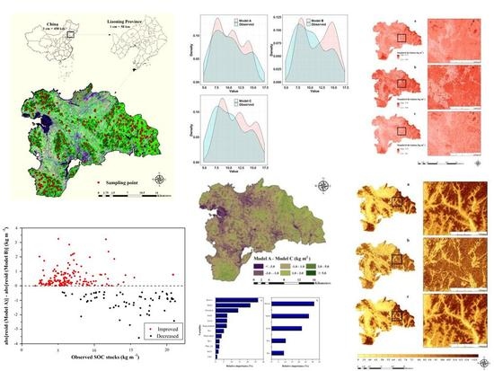
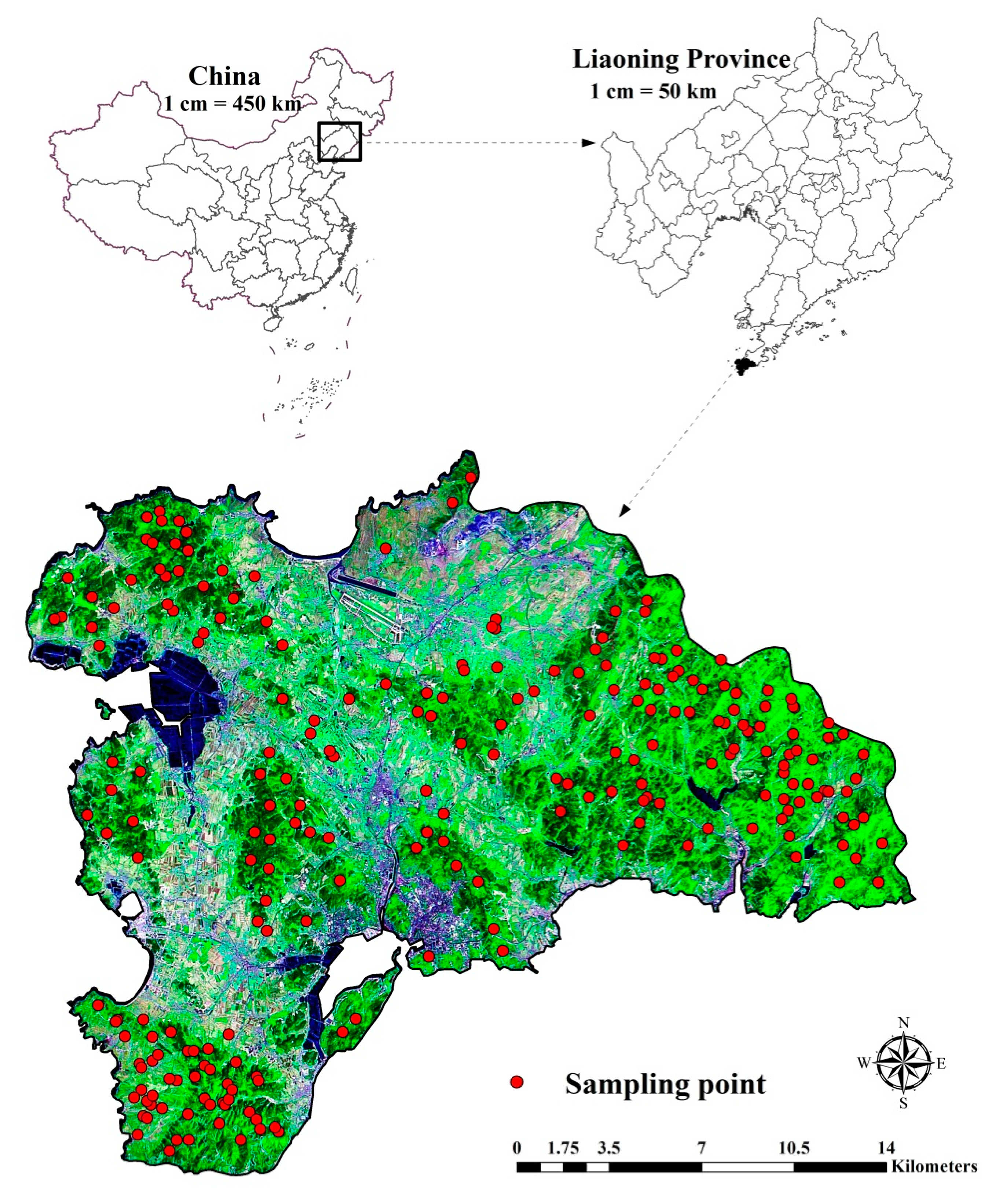
2.1. Study Area

The study area is located in Lushun District (38.72°–38.97°N, 121.08°–121.47°E)), Liaoning Province, Northeast China (Figure 1), and the southernmost part of Liaodong Peninsula. It is a municipal area of Dalian City, with a total area of 512 km². The terrain is low in the southwest and high in the northeast. Its elevation is 0–466 m above sea level. There are a number of geomorphic types in the area including middle and low mountains, hills, platforms, plains, and beaches. Its mean average temperature is 8–11 ℃, which is the warmest area in Northeast China. Its mean annual precipitation is between 550–1000mm, more in the east than in the west, more in the north than in the south, increasing from southwest to northeast. The area is dominated by forests, accounting for 53% of the total area. In addition, it is also a national scenic spot, National Nature Reserve and National Forest Park. Its main plant communities are coniferous forest, coniferous broad-leaved mixed forest, deciduous broad-leaved forest, artificial broad-leaved forest, deciduous broad-leaved shrub, shrub grass, non-zonal vegetation and agricultural vegetation. Its main soil types in this area are Cambisols (59%) and Fluvisols (17%) (World soil resource reference base) [25].

2.2. Sampling Strategy and Experimental Method

Due to the abundant forest area (53.1% of the area) and the limited funding and rough roads, extensive field sampling is impractical. In order to truly and accurately reflect the spatial characteristics of SOC stocks, the purpose sampling method [26] is used to design sampling points in this study. According to the corresponding relationship between soil properties and soil forming environment, the method assumes that the soil formed in a similar environment is similar [27]. The fuzzy c-means clustering method is used to cluster the main environmental factors such as slope gradient, slope aspect, elevation, mean annual temperature, mean annual precipitation and normalized vegetation index. According to the fuzzy membership value of each point in the combination of environmental factors, the representative grid of the corresponding category of environmental combination of each point and the accessibility degree of sample points are determined [28]. Finally, the high representative points are selected as the design sample points in combination with the vegetation type map [27]. Twenty-four clustering results were generated, and 8–10 samples were collected in each category, we obtained a total of 236 points in 2016. In order to determine the bulk density of soil, the undisturbed samples of 100 cm³ cores were collected in the center of soil layer. The samples were numbered and bagged respectively, and brought back to the laboratory for air drying before sample treatment; the bagged soil sample was dried by natural air, weighed, ground and passed through a nylon screen with a diameter of 2 mm. Soil samples were pretreated and measured in the Key Laboratory of agricultural resources and environment of Liaoning Province to determine SOC (Potassium dichromate sulfuric acid digestion method). Cores were dried at 105 ℃ for 48 h for soil bulk density measurement.

2.3. Environmental Data

In this study, 12 environmental variables representing multispectral remote sensing, topography and climate were selected. Since the data were obtained from different departments, we resampled them to raster data with a 30 m spatial resolution in ArcGIS 10.2. High precision environment variable is one of the essential conditions for accurate prediction of SOC stocks. The environment variable with high spatial resolution can provide more detailed attribute information, but the 30 m of spatial resolution is enough to reflect the distribution characteristics of SOC stocks in the area.

2.3.1. Multispectral Remote Sensing Variables

L1T level Landsat-8 imageries were acquired from one image (Path-row: 120-33) downloaded from the United States Geological Survey (USGS) covering the spatial domain of study area from July to September 2016. In order to ensure image quality and avoid the interference of cloud on model prediction, the cloudiness value error of the downloaded image data is controlled within less 10%. The Environment for Visualizing Images (ENVI) Fast Line-of-sight Atmospheric Analysis of Spectral Hypercubes (FLAASH) atmospheric correction method was used to correct the multispectral remote sensing data. We used a bilinear interpolation method to resample these data to raster format with a 30m spatial resolution in ArcGIS 10.2. The bilinear interpolation method takes the distance from the sampling point to the surrounding 4 neighborhood pixels to calculate the grid value. The grid value of the pixel is obtained by interpolation in Y direction (or X direction) and then in X direction (or Y direction). The boundary cleaning and main filtering tools were used to generalize the edges of the regions in the grid. According to the value of the neighborhood in each position, the edge was smoothed by expanding and contracting the boundary, or increasing or reducing the area [29]. The selected multispectral remote sensing variables include green band (B_GREEN) (0.52–0.60 μm), red band (B_RED) (0.63–0.69μm), near-infrared band (B_NIR) (0.77–0.90 μm), normalized difference vegetation Index (NDVI), and soil adjusted vegetation index (SAVI). Three selected bands were attributed to the fact that they could represent the growth and biomass of vegetation, and the images of ground objects were rich, distinct, and well-organized, and were used for vegetation classification and water body recognition [16]. NDVI is widely used in the detection of vegetation growth state, and the closer its value is to 1, the better the vegetation growth. Huete [30] proposed soil adjusted vegetation index (SAVI) based on NDVI and a large number of observation data to reduce the impact of soil background. Huete’s research [30] was conducted for the grassland and cotton fields, when L is 0.5, SAVI had a better effect on eliminating soil reflectance. NDVI and SAVI were calculated as follows:

$$NDVI=\left(B_{NIR}-B_{RED}\right)/\left(B_{NIR}+B_{RED}\right)$$

(1)

$$SAVI=\left(B_{NIR}-B_{RED}\right)\left(1+L\right)/\left(B_{NIR}+B_{RED}+L\right)\mathrm{L}=0.5$$

(2)

where B_NIR and B_RED were expressed as near-infrared band and red band; L is a parameter with the change of vegetation density, the value range is 0–1, the value for this study is set to 0.5.

2.3.2. Topographic Variables

Topographic variables data come from the Shuttle Radar Topography Mission and Digital Elevation Model (SRTM DEM) with a 30 m resolution. Due to the limitation of the accuracy of Space Surveying and mapping, only medium and small scale map data could be produced in the past. SRTM is a joint measurement mission carried out by the National Aeronautics and Space Administration (NASA), the national imaging and Mapping Agency (NIMA) of the United States Department of defense, Italy and Germany. From 11 to 22 February 2000, this survey mission acquired radar image data of about 119 million km² between 60°N and 60°S, covering more than 80% of the global land surface. Five terrain variables are selected in this study. Based on SRTM DEM data, four terrain variables are derived by using Arc GIS 10.2 software, which are elevation, slope gradient, slope aspect, and plan curvature. Topographic wetness index (TWI) is extracted by system for automated geoscientific analysis (SAGA) GIS [31] software.

2.3.3. Climatic Variables

Climate data were obtained from China Meteorological Science Data Sharing Service System (http://cdc.cma.gov.cn/), including MAP and MAT. Through collecting the MAT and MAP of 673 meteorological stations in China in 30 years (from 1980 to 2020 calculated by monthly average value), the raster data with 1 km resolution is generated by Kriging interpolation. Finally, the raster data were resampled to generate a resolution of 30 m by using the nearest neighbor principle, and the altitude data were used to correct it in ArcGIS 10.2.

2.4. Boosted Regression Tree

In this study, the BRT model proposed by Friedman et al. [16] was selected to predict the topsoil SOC stocks of a forest ecosystem in Northeast China. The BRT method had two technical components: boosting technology and regression tree [15]. Regression tree (RT) uses a set of predictive variables to analyze response variables, and applies binary segmentation to fit the simple model to each result part [17]. Boosting technology is to iterate multiple regression trees to make common decisions [7]. When the square error loss function is used, each regression tree drew conclusions and provided residuals of all previous trees, and a current residuals regression tree is obtained by fitting. Regression tree is the accumulation of regression trees generated in the whole iterative process [16]. The BRT model is more accurate and fast through gradient lifting technology and multiple data optimization.

In this study, the BRT model was constructed by “gem” package [32] in R language environment. In BRT model, four parameters required users to set: learning rate (LR), tree complexity (TC), bag fraction (BF), and tree number (TN) [17]. LR represents the contribution of each tree to the growth of the model [16]. TC represents the scale of the control tree and the interaction between variables [8]. BF sets the observation proportion for selecting variables [16]. NT represents the scale of the tree based on the combination of LR and TC [17]. We tested different combinations of LR, TC, BF, and NT. The optimal parameter combination was the one that provided the minimum predictive deviation. Finally, we determined the optimal parameter settings LR, TC, BF, and NT as 0.025, 12, 0.75, and 1200, respectively, so that the model demonstrated the best performance.

2.5. Model Evaluation

In order to evaluate the prediction performance of the three constructed BRT models on the spatial distribution of SOC stocks, we choose a common test method, namely the 10-fold cross validation technology. The dataset was divided into ten parts, nine of which were used as training data and one as test data in turn. In order to evaluate the performance of the BRT model, four indexes are calculated, including error (MAE), root mean square error (RMSE), coefficient of determination (R²) and Lin’s concordance correlation coefficient (LCCC) [33], in R software 3.2.2. Their specific formulae are as follows:

$$MAE=\frac{1}{n}{\displaystyle \sum _{i=1}^n\left|x_i-y_i\right|}$$

(3)

$$RMSE=\sqrt{\frac{1}{n}{\displaystyle \sum _{i=1}^n{\left(x_i-y_i\right)}^2}}$$

(4)

$$R^2=\frac{{\displaystyle \sum _{i=1}^n{\left(x_i-{\overline{y}}_i\right)}^2}}{{\displaystyle \sum _{i=1}^n{\left(y_i-{\overline{y}}_i\right)}^2}}$$

(5)

$$LCCC=\frac{2r{\partial }_x{\partial }_y}{{\partial }_x^2+{\partial }_y^2+{\left(\overline{x}+\overline{y}\right)}^2}$$

(6)

where x_i and y, represent the predicted value and measured value at point i; $\overline{x}$ and $\overline{y}$ are the mean of the predicted and measured values; ∂_x and ∂_y represent the variance of the predicted and measured values; n is the number of sampling sits; r is the correlation coefficient between the predicted value and the measured value.

3. Results

3.1. Descriptive Statistics

The statistical results between SOC stocks and environmental variables at each sampling site are shown in

Table 1. Summary statistics of soil organic carbon (SOC) stocks (0–30 cm) and environmental variables at samples sites.

Category	Property	Unit	Min.	Median	Mean	Max.	SD	Skewness	Kurtosis
Soil	SOC stocks	kg m−2	1.37	9.30	9.07	20.86	3.95	0.37	−0.93
Remote sensing imagery	BGREEN	digital number	0.00	45.72	71.92	217.13	66.14	0.70	−0.93
	BRED	digital number	5.97	182.90	162.89	253.22	68.31	−0.58	−0.84
	BNIR	digital number	0.00	38.77	64.57	218.68	63.73	0.92	−0.43
	NDVI		0.15	0.38	0.40	0.56	0.08	−0.18	0.30
	SAVI		0.12	0.46	0.43	0.77	0.15	−0.43	0.58
Topography	Elevation	m	4.96	52.63	65.51	272.63	49.78	1.66	3.56
	Slope gradient	degree	0.00	6.81	9.33	34.10	8.20	1.03	0.38
	Slope aspect	degree	0.00	223.20	194.53	350.83	101.29	−0.44	−0.94
	Plan_cur		−1.83	0.00	0.03	1.51	0.49	−0.44	2.73
	TWI		2.45	4.27	4.70	10.07	1.51	1.00	1.32
Climate	MAT	degree celsius	9.44	10.43	10.34	10.84	0.23	−1.32	2.73
	MAP	mm	600.95	602.64	606.05	618.14	3.85	1.53	1.85

Notes: SOC, Soil organic carbon; B_GREEN, green band; B_RED, red band 4; B_NIR, near-infrared band; NDVI, normalized difference vegetation index; SAVI, soil adjusted vegetation index; Plan_cur, plan curvature; TWI, topographic wetness index; MAP, mean annual precipitation; MAT, mean annual temperature; SD, standard deviation; Min., minimum; Max., maximum.

. The average value of SOC stocks is 9.07 kg m⁻², and the coefficient of skewness is 0.37 kg m⁻², indicating that SOC presents a slightly skewed distribution. In addition, since SOC stocks are not evenly distributed on both sides of the average values, we Ln-transformed the SOC data s for later modeling and simulation. The SD of the sampling point is 3.95 kg m⁻², and it is lower than the average value.

In order to explore the relationship between Log-SOC stocks and environmental variables, we calculated the Pearson correlation coefficient among them, as shown in

Table 2. Pearson correlation analysis between Ln-transformed SOC stocks and environmental variables based on 236 samples.

Property	SOC Stocks	BGREEN	BRED	BNIR	NDVI	SAVI	Elevation	Slope Gradient	Slope Aspect	Plan_cur	TWI	MAT
BGREEN	−0.57 **
BRED	−0.33 **	0.33 **
BNIR	−0.61 **	0.63 *	0.31 **
NDVI	0.71 **	−0.71 **	0.52 **	−0.47 **
SAVI	0.63 **	−0.63 **	0.44 **	−0.36 **	0.67 **
Elevation	0.70 **	−0.43 **	−0.23 *	−0.49 **	0.17	0.16
Slope gradient	0.68 **	−0.52 **	−0.12	−0.53 **	0.08	0.09	0.63 **
Slope aspect	0.17	−0.06	0.06	−0.14	−0.05	−0.08	0.19	0.17
Plan_cur	0.07	−0.09	−0.08	−0.04	0.14	0.13	0.13	0.05	−0.07
TWI	−0.59 **	0.53 **	0.24 *	0.41 **	−0.06	−0.06	−0.53 **	−0.73 **	−0.21 *	−0.19
MAT	−0.35 **	0.27 **	−0.06	0.21 *	−0.16 *	−0.21 **	−0.37 **	−0.34 **	0.09	0.07	0.21 *
MAP	0.28 **	−0.13	0.22 *	−0.14	0.15 *	0.23 **	0.31 **	0.45 **	0.16	−0.04	−0.27 *	−0.13

Notes: p < 0.05 shown in “*”; p < 0.01 shown in “**”; SOC, Soil organic carbon; B_GREEN, green band; B_RED, red band 4; B_NIR, near-infrared band; NDVI, normalized difference vegetation index; SAVI, soil adjusted vegetation index; Plan_cur, plan curvature; TWI, topographic wetness index; MAP, mean annual precipitation; MAT, mean annual temperature.

. NDVI (r = 0.71), SAVI (r = 0.63), elevation (r = 0.70), slope gradient (r = 0.68), and MAP (r = 0.28) were positively correlated with SOC stocks. Correspondingly, SOC stocks was negatively correlated with B_GREEN (r = −0.57), B_RED (r = −0.33), B_NIR (r = −0.61), TWI (r = −0.59), and MAT (r = −0.35). Surprisingly, the correlation between multispectral remote sensing variables and SOC stocks was significant in this study.

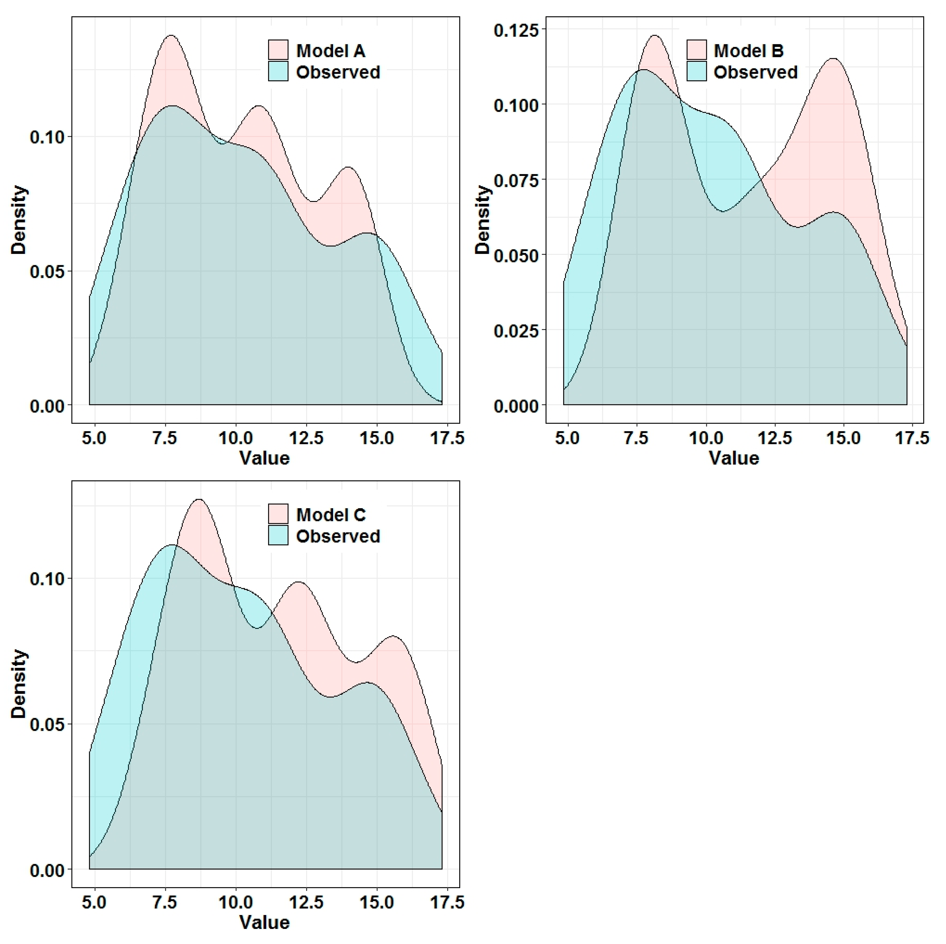
3.2. Model Performance

We compared the spatial prediction performance of three BRT models with different variable combinations to predict the topsoil SOC stocks in Lushun, where is mainly controlled by forest ecosystems. The accuracy verification results are shown in

Table 3. Predictive quality of three boosted regression trees (BRT) models for SOC stocks.

Model	Index	Min.	1st Quartile	Median	Mean	3rd Quartile	Max.
Model A	MAE	0.05	0.06	0.06	0.06	0.06	0.06
	RMSE	0.07	0.07	0.07	0.07	0.08	0.08
	R2	0.64	0.65	0.65	0.65	0.66	0.67
	LUCC	0.86	0.87	0.87	0.87	0.87	0.87
Model B	MAE	0.14	0.15	0.15	0.15	0.15	0.15
	RMSE	0.18	0.19	0.19	0.19	0.19	0.20
	R2	0.51	0.52	0.53	0.53	0.54	0.55
	LUCC	0.70	0.71	0.72	0.72	0.72	0.73
Model C	MAE	0.10	0.10	0.10	0.11	0.11	0.11
	RMSE	0.12	0.13	0.13	0.13	0.13	0.13
	R2	0.59	0.60	0.61	0.61	0.63	0.64
	LUCC	0.80	0.81	0.81	0.81	0.81	0.81

Notes: Model A, full variables model (multispectral remote sensing variables + topographic variable + climatic variables); Model B, only topographic and climatic variables; Model C, only multispectral remote sensing variables; MAE, the mean absolute error; RMSE, the root mean squared error; R², the coefficient of determination; LCCC, Lin’s concordance correlation coefficient.

. Among all models, the full variable model presents the best prediction performance, followed by the only multispectral remote sensing data model, and the finally topographic and climatic variables model, which could explain the spatial variation of 65%, 61%, and 53% SOC stocks in the region, respectively. The results showed that, using the multispectral remote sensing variable, the prediction model (MAE = 0.11, RMSE = 0.13, R² = 0.61, and LUCC = 0.81) could catch up with the full-variable prediction model (MAE = 0.06, RMSE = 0.07, R² = 0.65, and LUCC = 0.87). Model A and Model C were significantly better than model B (no multispectral remote sensing data). The density distribution map of the observed and predicted values of the sampling sites further confirms this finding (Figure 2). Model A and Model C showed a similar distribution trend, while Model C showed a steeper distribution pattern.

In order to further evaluate the performance of the model, we calculated the absolute residuals of Model A and Model B at all sampling sites. We found that only a small part of the sampling sites showed a decreasing trend and showed a small variation (Figure 3). In addition, we subtracted the final prediction results of Model A and Model C using raster calculation module in ArcGIS 10.1, and formed the prediction difference diagram of the two methods. The average and SD values of the difference results were 0.32 kg m⁻² and 4.67 kg m⁻² respectively, which further showed that the difference between Model A and Model C in the prediction of SOC stocks was not obvious in the region.

To further evaluate the prediction potential of multispectral remote sensing variables, we calculated the difference between the spatial mapping results of full variable model and only multispectral remote sensing variables mode (Figure 4). As shown in Figure 4, only some areas showed a downward trend, and the differences between them were slight. In addition, we also calculated the standard deviation (SD) of a hundred iterations of the three models to further evaluate the performance and uncertainty. From Figure 5, it could be seen that all models produce lower SD. The mean SD of Model A, Model B and Model C were 0.17, 0.36, and 0.23 kg m⁻², respectively.

3.3. Relative Importance of Environment Variables

Model A (full environment variable) was iterated 100 times and the mean relative importance (RI) of each environment variable was calculated. For the convenience of analysis, the relative importance of each environment variable was reduced to 100%. From Figure 6a, we found that NDVI, SAVI, B3, elevation, TWI and MAP were the main environmental variables (accounting for 75% of the total relative importance) that affect the spatial variation of SOC stocks in this region. In addition, multispectral remote sensing variables played an important role in Model A (63%), followed by topographic variables (28%) and climatic variables (9%). In addition, in Model C with only multispectral variables, B_GREEN (31%) showed the highest relative importance, followed by NDVI (27%), SAVI (22%), B_NIR (11%), and B_RED (9%) (Figure 6b).

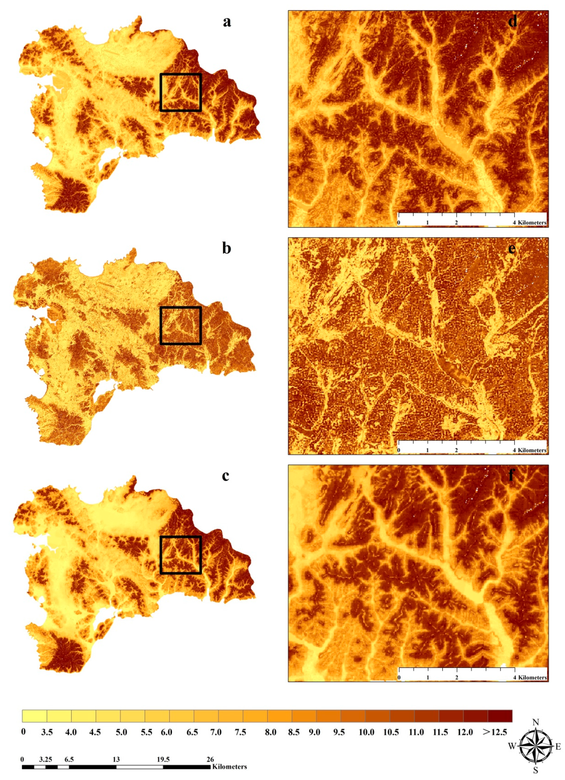
3.4. Spatial Distribution of SOC Stocks

Different from a single linear model, the results of each iteration with the BRT model were different. Therefore, we selected the three BRT models by iterating 100 times and calculating their average values as the final prediction results. Figure 7 showed the final prediction results of the three models. The average prediction results of Model A, Model B, and Model C were 8.99, 10.22, and 9.32 kg m⁻², respectively.

4. Discussion

4.1. Effect of Multispectral Remote Sensing Variables on SOC Stocks

Multispectral remote sensing variables were the powerful and effectual variables in the full variables model, which showed that multispectral remote sensing data can predict forest topsoil SOC stocks, which is consistent with many previous research results [23,24,34,35,36,37,38]. In the Bale Mountains, Ethiopia, Yimer et al. [24] concluded that vegetation was the main source of SOC stocks and affected its distribution, and there was a significant positive correlation between vegetation and SOC stocks, which has been certified in this study (Table 2). B_GREEN and NDVI were efficient variables to characterize vegetation density and biomass, so they were important predictors in predicting of SOC stocks [17]. SAVI is very sensitive to the change of soil background [30]. Many studies showed that there were some potential applications of multispectral remote sensing data in SOC stocks mapping with better natural vegetation coverage areas [7,17,34,35,36,37,38,39]. B_GREEN is a better predictor than NDVI and SAVI in the full variable model, although many scholars considered NDVI was a more effective and powerful predictor [35,37]. Therefore, B_GREEN should be recommended as an influential factor in the future studies, especially in the areas with dense vegetation coverage. In addition, the Pearson correlation coefficients of B_GREEN, NDVI, and SAVI with SOC stocks are −0.57, 0.71, and 0.63, respectively, which indirectly proved that they had potential value in mapping of SOC stocks. In Liaoning Province, China, Qi et al. [7] pointed out that SAVI was a highly effective and powerful predictor in the prediction of topsoil SOC in forest ecosystem. Yang et al. [17] found B_GREEN and NDVI were the most important remote sensing variables in the prediction of topsoil SOC in the Tibetan Plateau. Gomez et al. [38] conducted multispectral remote sensing data were effective to deduce the spatial characteristics information of SOC stocks. Kim and Grunwald [23] also proved that multispectral remote sensing related variables could represent the spatial variability and quantity of soil carbon. In Tanzania, Winowiecki et al. [39] found that the spatial distribution pattern of SOC stocks was closely related to vegetation types and coverage. However, we would like to point out that, due to low-density sampling, the sampling in the study may not be representative. The results might overemphasize the importance of some variables in the model and increased the uncertainty of model prediction.

Terrain related variables are good predictors of SOC stocks in complex terrain change areas [8,17]. As one of the five soil-forming factors [40], topographic variables as a common variable in digital soil mapping (DSM) were selected as the main prediction factor in this study. In the process of SOC stocks prediction, the relative importance of terrain related variable was lower than that of multi spectral remote sensing related variable, which was consistent with previous research results [7,8,17,34]. Yang et al. [17] considered that, in the area with abundant vegetation, the influence of terrain elements on SOC stocks was integrated by remote sensing variables. Elevation had the most important influence on the spatial distribution of SOC stocks among all topographic variables. It was observed that the terrain was highly variable in the region, and the elevation could adjust the role of local microclimate [38]. Our research confirmed that the climate characteristics affected by elevation were significantly correlated with MAP (0.35) and MAT (−0.28)

As the main climatic factors, MAP and MAT were widely used in the spatial simulation of SOC stocks [8,36]. MAP was the fourth most important predictor in the full variable BRT model (Figure 3) and played a more important role than MAT in predicting SOC stocks. In the mountain ecosystem, the hydrothermal condition affected the decomposition and accumulation of organic matter, indirectly impacting the spatial distribution characteristics of SOC stocks in those regions [17]. At the micro-level, the increase of forest productivity means a large amount of input of soil organic matter [37]. However, low temperature will slow down the decomposition rate of SOC. Although SOC stocks had a good correlation with MAP and MAT (Table 2), they were generated by data interpolation of 673 meteorological stations in China. Its spatial resolution was 1000 m, which is too coarse to characterize the spatial distribution of SOC stocks. In contrast, high spatial resolution remote sensing data could improve the spatial distribution characteristics of SOC stocks in the prediction area, because the data contain more detailed, higher resolution vegetation coverage information.

Our research concluded that the multispectral remote sensing data are effective to map SOC stocks in high-density vegetation coverage area. Many studies have a similar conclusion regarding the major controls of SOC distribution [7,34,35,36,37]. For instance, in the Qilian Mountains of China, Yang et al. [17] used three bands of Landsat-5 TM (B_GREEN, B_RED, and B_NIR) and random forest to predict SOC and obtain higher prediction accuracy in the natural field (R² = 0.72). Similarly, we used three multispectral remote sensing bands (B_GREEN, B_RED, and B_NIR), NDVI and SAVI constructed a BRT model to predict the spatial distribution of SOC stocks in this densely covered natural vegetation with a high prediction accuracy.

4.2. Uncertainty in Current Research

The uncertainty of the three BRT model predictions was shown in Figure 5. These results revealed that the BRT model had excellent performance in predicting the spatial distribution of SOC stocks. However, there were still some uncertainties in this study. First, this study was divided into different groups to collect and analyze samples, so there might be sampling errors and experimental errors. Second, all environment variables were resampled to 30 m spatial resolution in ArcGIS 10.2 using a bilinear interpolation method, which will cause some method errors. Third, the accuracy and scale of the environment data obtained from different platforms were different, which resulted in subsequent modeling errors. Finally, this study was limited to the estimation of SOC in the topsoil (0–30 cm) forest, which will lead to the underestimation of SOC stocks in the region. In the forest ecosystem, the SOC stocks were generally stored in the deeper soil.

In addition, despite the success of using multispectral remote sensing data in this study, there were still some aspects worthy of special attention. These include: (1) affected by the terrain and clouds, the high-altitude areas were prone to produce shadows in the process of segmentation, so these reflectivity errors were large in satellite imageries data; (2) terrain variables have proved to be a powerful predictor of the spatial distribution of SOC stocks, especially in the forest ecosystem with obvious terrain change and dense vegetation coverage. Therefore, we recommend that the terrain related variables shall be added to the remote sensing prediction model for future forest organic carbon stock mapping.

Although the environmental conditions, sampling strategies, and sampling methods in this study were different from previous studies, the performance of the BRT model prediction was comparable to those studies. In Denmark, Adhikari et al. [41] used a regression kriging model and 18 environmental variables as predictors to model the vertical distribution of SOC content, and which only explained 23%–43% of SOC content variability. Were et al. [42] used the RF model to predict the SOC stocks and concluded that the RF model could explain 52% of the spatial changes of SOC in an Afromontane landscape. In Liaoning Province of China, Wang et al. [43] used a BRT model and nine environmental variables to predict the spatial distribution of SOC stocks of topsoil forests and could explain 58% of the spatial change of SOC stocks.

5. Conclusions

By comparing three BRT models, the best prediction model of topsoil SOC stocks in Liaoning coastal forest ecosystem was obtained. We found that using multispectral remote sensing variables alone, the model was not inferior to the full variable model, suggesting that using the remote sensing data is efficient and robust for predicting topsoil SOC stocks. The addition of climatic and topographic variables could improve the performance of the prediction model to some extent. In the selection of environmental variables, the use of multispectral remote sensing variables had a high practical significance in the spatial simulation of topsoil SOC stocks. Our study suggests that, in the future mapping of topsoil SOC stocks, especially in the forest ecosystem area with dense vegetation, appropriate multispectral remote sensing variables should be selected. Our accurate mapping of SOC stocks shall have great significance for studying the carbon cycle, soil fertility maintenance, and the ecological environment protection of forest ecosystems in our study region.

References

1. Liski, J.; Perruchoud, D.; Karjalainen, T. Increasing carbon stocks in the forest soils of western Europe. For. Ecol. Manag. 2002, 169, 159–175. [Google Scholar] [CrossRef]
2. Rapalee, G.; Trumbore, S.E.; Davidson, E.A.; Harden, J.W.; Veldhuis, H. Soil carbon stocks and their rates of accumulation and loss in a boreal forest landscape. Glob. Biogeochem. Cy. 1998, 12, 687–701. [Google Scholar] [CrossRef] [Green Version]
3. Fujisaki, K.; Perrin, A.S.; Desjardins, T.; Bernoux, M.; Balbino, L.C.; Brossard, M. From forest to cropland and pasture systems: A critical review of soil organic carbon stocks changes in Amazonia. Glob. Chang. Biol. 2015, 21, 2773–2786. [Google Scholar] [CrossRef] [PubMed] [Green Version]
4. Grinand, C.; Le Maire, G.; Vieilledent, G.; Razakamanarivo, H.; Razafimbelo, T.; Bernoux, M. Estimating temporal changes in soil carbon stocks at ecoregional scale in Madagascar using remote-sensing. Int. J. Appl. Earth Obs. 2017, 54, 1–14. [Google Scholar] [CrossRef]
5. Willaarts, B.A.; Oyonarte, C.; Muñoz-Rojas, M.; Ibáñez, J.J.; Aguilera, P.A. Environmental factors controlling soil organic carbon stocks in two contrasting Mediterranean climatic areas of southern Spain. Land. Degrad. Dev. 2016, 27, 603–611. [Google Scholar] [CrossRef]
6. Conforti, M.; Lucà, F.; Scarciglia, F.; Matteucci, G.; Buttafuoco, G. Soil carbon stock in relation to soil properties and landscape position in a forest ecosystem of southern Italy (Calabria region). Catena 2016, 144, 23–33. [Google Scholar] [CrossRef]
7. Qi, L.; Wang, S.; Zhuang, Q.; Yang, Z.; Bai, S.; Jin, X.; Lei, G. Spatial-temporal changes in soil organic carbon and pH in the Liaoning Province of China: A modeling analysis based on observational data. Sustainability 2019, 11, 3569. [Google Scholar] [CrossRef] [Green Version]
8. Wang, S.; Wang, Q.; Adhikari, K.; Jia, S.; Jin, X.; Liu, H. Spatial-temporal changes of soil organic carbon content in Wafangdian, China. Sustainability 2016, 8, 1154. [Google Scholar] [CrossRef] [Green Version]
9. Ottoy, S.; De Vos, B.; Sindayihebura, A.; Hermy, M.; Van Orshoven, J. Assessing soil organic carbon stocks under current and potential forest cover using digital soil mapping and spatial generalisation. Ecol. Indic. 2017, 77, 139–150. [Google Scholar] [CrossRef]
10. Rasel, S.M.M.; Groen, T.A.; Hussin, Y.A.; Diti, I.J. Proxies for soil organic carbon derived from remote sensing. Int. J. Appl. Earth Obs. 2017, 59, 157–166. [Google Scholar] [CrossRef]
11. Gahlod, N.S.S.; Jaryal, N.; Roodagi, M.; Dhale, S.A.; Kumar, D.; Kulkarni, R. Soil organic carbon stocks assessment in Uttarakhand State using remote sensing and GIS technique. Int. J. Curr. Microbiol. Appl. Sci. 2019, 8, 1646–1658. [Google Scholar] [CrossRef]
12. Chen, F.; Kissel, D.E.; West, L.T.; Adkins, W. Field-scale mapping of surface soil organic carbon using remotely sensed imagery. Soil Sci. Soc. Am. J. 2000, 64, 746–753. [Google Scholar] [CrossRef] [Green Version]
13. Fox, G.A.; Sabbagh, G.J. Estimation of soil organic matter from red and near-infrared remotely sensed data using a soil line Euclidean distance technique. Soil Sci. Soc. Am. J. 2000, 66, 1922–1929. [Google Scholar] [CrossRef]
14. Hill, J.; Schütt, B. Mapping complex patterns of erosion and stability in dry Mediterranean ecosystems. Remote Sens. Enviro. 2000, 74, 557–569. [Google Scholar] [CrossRef]
15. Elith, J.; Leathwick, J.R.; Hastie, T. A working guide to boosted regression trees. J. Anim. Ecol. 2008, 77, 802–813. [Google Scholar] [CrossRef]
16. Friedman, J.; Hastie, T.; Tibshirani, R. Additive logistic regression: A statistical view of boosting. Ann. Stat. 2000, 28, 337–407. [Google Scholar] [CrossRef]
17. Yang, R.M.; Zhang, G.L.; Liu, F.; Lu, Y.Y.; Yang, F.; Yang, F.; Yang, M.; Zhao, Y.G.; Li, D.C. Comparison of boosted regression tree and random forest models for mapping topsoil organic carbon concentration in an alpine ecosystem. Ecol. Indic. 2016, 60, 870–878. [Google Scholar] [CrossRef]
18. Carslaw, D.C.; Taylor, P.J. Analysis of air pollution data at a mixed source location using boosted regression trees. Atmos. Environ. 2009, 43, 3563–3570. [Google Scholar] [CrossRef]
19. Yoon, L.C.; Pedro, J.; Leitão, T.L. Assessment of land use factors associated with dengue cases in Malaysia using Boosted Regression Trees. Spat. Spatio Tempor. Epidemiol. 2014, 10, 75–84. [Google Scholar]
20. De’Ath, G. Boosted trees for ecological modeling and prediction. Ecology 2007, 88, 243–251. [Google Scholar] [CrossRef]
21. Pouteau, R.; Rambal, S.; Ratte, J.P.; Gogé, F.; Joffre, R.; Winkel, T. Downscaling MODIS-derived maps using GIS and boosted regression trees: The case of frost occurrence over the arid Andean highlands of Bolivia. Remote Sens. Environ. 2011, 115, 117–129. [Google Scholar] [CrossRef] [Green Version]
22. Lampa, E.; Lind, L.; Lind, P.M.; Bornefalk-Hermansson, A. The identification of complex interactions in epidemiology and toxicology: A simulation study of boosted regression trees. Environ. Health 2014, 13, 57. [Google Scholar] [CrossRef] [PubMed] [Green Version]
23. Kim, J.; Grunwald, S. Assessment of carbon stocks in the topsoil using random forest and remote sensing images. J. Environ. Qual. 2016, 45, 1910–1918. [Google Scholar] [CrossRef] [PubMed]
24. Yimer, F.; Ledin, S.; Abdelkadir, A. Soil organic carbon and total nitrogen stocks as affected by topographic aspect and vegetation in the Bale Mountains, Ethiopia. Geoderma 2006, 135, 335–344. [Google Scholar] [CrossRef]
25. Schad, P.; Van Huyssteen, C.; Micheli, E. International Soil Classification System for Naming Soils and Creating Legends for Soil Maps; World Reference Base for Soil Resources: Rome, Italy, 2014; Volume 106, pp. 246–385. [Google Scholar]
26. Zhu, A.X.; Yang, L.; Li, B.; Qin, C.; English, E.; Burt, J.E.; Zhou, C.H. Purposive sampling for digital soil mapping for areas with limited data. In Digital Soil Mapping with Limited Data; Hartemink, A.E., McBratney, A.B., de Lourdes, M.-S., Eds.; Springer: Amsterdam, The Netherlands, 2008; Volume 8, pp. 233–245. [Google Scholar]
27. Yang, L.; Zhu, A.; Qin, C.; Li, B.; Pei, T. A soil sampling method based on representativeness grade of sampling points. Acta Pedol. Sin. 2011, 48, 938–946. [Google Scholar]
28. Yang, L.; Zhu, A.; Qin, C.; Li, B.; Pei, T.; Liu, B. Soil property mapping using fuzzy membership-a case study of a study area in Heshan Farm of Heilongjiang Province. Acta Pedol. Sin. 2009, 46, 9–15. [Google Scholar]
29. Sundaresan, A.; Varshney, P.K.; Arora, M.K. Robustness of change detection algorithms in the presence of registration errors. Photogramm. Eng. Rem. Sens. 2007, 73, 375–383. [Google Scholar] [CrossRef]
30. Huete, A.R. A soil-adjusted vegetation index (SAVI). Remote Sens. Enviro. 1988, 25, 295–309. [Google Scholar] [CrossRef]
31. Olaya, V.F. A Gentle Introduction to Saga GIS.; The SAGA User Group eV: Göttingen, Germany, 2004. [Google Scholar]
32. Gbm: Generalized Boosted Regression Models, R Package Version 1.6-3. Available online: http://127.0.0.1:31000/library/gbm/html/gbm-package.html (accessed on 26 November 2007).
33. Lin, L. A concordance correlation coefficient to evaluate reproducibility. Biometrics 1989, 45, 255–268. [Google Scholar] [CrossRef]
34. Wang, B.; Waters, C.; Orgill, S.; Gray, J.; Cowie, A.; Clark, A.; Li Liu, D. High resolution mapping of soil organic carbon stocks using remote sensing variables in the semi-arid rangelands of eastern Australia. Sci. Total Environ. 2018, 630, 367–378. [Google Scholar] [CrossRef]
35. Nyssen, J.; Temesgen, H.; Lemenih, M.; Zenebe, A.; Haregeweyn, N.; Haile, M. Spatial and temporal variation of soil organic carbon stocks in a lake retreat area of the Ethiopian Rift Valley. Geoderma 2008, 146, 261–268. [Google Scholar] [CrossRef]
36. Xu, X.; Liu, W.; Zhang, C.; Kiely, G. Estimation of soil organic carbon stock and its spatial distribution in the Republic of Ireland. Soil Use Manag. 2011, 27, 156–162. [Google Scholar] [CrossRef]
37. Chi, Y.; Shi, H.; Zheng, W.; Sun, J. Simulating spatial distribution of coastal soil carbon content using a comprehensive land surface factor system based on remote sensing. Sci. Total Environ. 2018, 628, 384–399. [Google Scholar] [CrossRef] [PubMed]
38. Gomez, C.; Rossel, R.A.V.; McBratney, A.B. Soil organic carbon prediction by hyperspectral remote sensing and field vis-NIR spectroscopy: An Australian case study. Geoderma 2008, 146, 403–411. [Google Scholar] [CrossRef]
39. Winowiecki, L.; Vågen, T.G.; Huising, J. Effects of land cover on ecosystem services in Tanzania: A spatial assessment of soil organic carbon. Geoderma 2016, 263, 274–283. [Google Scholar] [CrossRef] [Green Version]
40. Jenny, H. Factors of Soil Formation: A System of Quantitative Pedology; Beth, R., Ed.; Soil Science: Philadelphia, PA, USA, 1941; Volume 42, p. 415. [Google Scholar]
41. Adhikari, K.; Hartemink, A.E.; Minasny, B.; Kheir, R.B.; Greve, M.B.; Greve, M.H. Digital mapping of soil organic carbon contents and stocks in Denmark. PLoS ONE 2014, 9, e105519. [Google Scholar] [CrossRef] [PubMed]
42. Were, K.; Bui, D.T.; Dick, Ø.B.; Singh, B.R. A comparative assessment of support vector regression, artificial neural networks, and random forests for predicting and mapping soil organic carbon stocks across an Afromontane landscape. Ecol. Indic. 2015, 52, 394–403. [Google Scholar] [CrossRef]
43. Wang, S.; Zhuang, Q.; Yang, Z.; Yu, N.; Jin, X. Temporal and Spatial Changes of Soil Organic Carbon Stocks in the Forest Area of Northeastern China. Forests 2019, 10, 1023. [Google Scholar] [CrossRef] [Green Version]
Figure 1. Location of the study area and sampling points, which are superimposed on a 30-m resolution remote sensing image.
Remotesensing 12 00393 g001
Figure 2. Density plots of soil organic carbon stocks (kg m−2) derived from three boosted regression trees (BRT) models.
Remotesensing 12 00393 g002
Figure 3. Difference of absolute residual values between full variable model (Model A) and only topographic and climatic variables model (Model B). Decreased: prediction accuracy decreased; Improved: prediction accuracy increased.
Remotesensing 12 00393 g003
Figure 4. Difference map of soil organic carbon stocks (kg m−2) derived from full variable model (Model A) and only multispectral remote sensing variables (Model C).
Remotesensing 12 00393 g004
Figure 5. Standard deviation maps obtained by using three BRT models iterated 100 times. (a) full variables model (Model A); (b) topography and climate variables (Model B); and (c) only multispectral remote sensing variables (Model C); (df) areas covered with black boxes are detailed on the right.
Remotesensing 12 00393 g005
Figure 6. Relative importance of each prediction variable in full variable model (Model A) (a) and only multispectral remote sensing variables (Model C) (b). BGREEN, green band; BRED, red band 4; BNIR, near-infrared band; NDVI, normalized difference vegetation index; SAVI, soil adjusted vegetation index; Plan_cur, plan curvature; TWI, topographic wetness index; MAP, mean annual precipitation; MAT, mean annual temperature.
Remotesensing 12 00393 g006
Figure 7. Distribution maps of topsoil (0–30cm) organic carbon stocks (kg m−2) derived from three boosted regression tree (BRT) models. (a) full variables model (Model A); (b) topography and climate variables (Model B); and (c) only multispectral remote sensing variables (Model C); (df) areas covered with black boxes are detailed on the right.
Remotesensing 12 00393 g007