Article

Discriminative Feature Learning Constrained Unsupervised Network for Cloud Detection in Remote Sensing Imagery

State Key Laboratory of Integrated Service Networks, School of Telecommunications Engineering, Xidian University, Xi’an 710071, China
*
Author to whom correspondence should be addressed.
Submission received: 11 December 2019 / Revised: 15 January 2020 / Accepted: 20 January 2020 / Published: 1 February 2020
(This article belongs to the Special Issue Remote Sensing Image Restoration and Reconstruction)

Abstract

:
Cloud detection is a significant preprocessing step for increasing the exploitability of remote sensing imagery that faces various levels of difficulty due to the complexity of underlying surfaces, insufficient training data, and redundant information in high-dimensional data. To solve these problems, we propose an unsupervised network for cloud detection (UNCD) on multispectral (MS) and hyperspectral (HS) remote sensing images. The UNCD method enforces discriminative feature learning to obtain the residual error between the original input and the background in deep latent space, which is based on the observation that clouds are sparse and modeled as sparse outliers in remote sensing imagery. The UNCD enforces discriminative feature learning to obtain the residual error between the original input and the background in deep latent space, which is based on the observation that clouds are sparse and modeled as sparse outliers in remote sensing imagery. First, a compact representation of the original imagery is obtained by a latent adversarial learning constrained encoder. Meanwhile, the majority class with sufficient samples (i.e., background pixels) is more accurately reconstructed than the clouds with limited samples by the decoder. An image discriminator is used to prevent the generalization of out-of-class features caused by latent adversarial learning. To further highlight the background information in the deep latent space, a multivariate Gaussian distribution is introduced. In particular, the residual error with clouds highlighted and background samples suppressed is applied in the cloud detection in deep latent space. To evaluate the performance of the proposed UNCD method, experiments were conducted on both MS and HS datasets that were captured by various sensors over various scenes, and the results demonstrate its state-of-the-art performance. The sensors that captured the datasets include Landsat 8, GaoFen-1 (GF-1), and GaoFen-5 (GF-5). Landsat 8 was launched at Vandenberg Air Force Base in California on 11 February 2013, in a mission that was initially known as the Landsat Data Continuity Mission (LDCM). China launched the GF-1 satellite. The GF-5 satellite captures hyperspectral observations in the Chinese Key Projects of High-Resolution Earth Observation System. The overall accuracy (OA) values for Images I and II from the Landsat 8 dataset were 0.9526 and 0.9536, respectively, and the OA values for Images III and IV from the GF-1 wide field of view (WFV) dataset were 0.9957 and 0.9934, respectively. Hence, the proposed method outperformed the other considered methods.

Graphical Abstract

1. Introduction

Remote sensing imaging technology such as multispectral (MS) imaging and hyperspectral (HS) imaging can perceive targets or natural phenomena remotely [1,2,3]. Depending on the wide-scale monitoring capability, remote sensing images have been successfully applied to target detection [4], anomaly detection [5], and classification [6]. In [4], the current scenario and challenges of hyperspectral target detection are reviewed. Yuan et al. [5] introduced a method of hyperspectral anomaly detection that uses image pixel selection. Based on deep learning, the method in [6] increases the classification accuracy.
However, due to the significant impact of the atmospheric density and the cloud layer on the image acquisition process, most remote sensing images are inevitably polluted by clouds to different degrees [7], thereby resulting in inaccurate spectral characteristics of targets or natural phenomena, which reduces the exploitability of the image [8]. Consequently, cloud detection is an important preprocessing step for the promotion of the subsequent application and the improvement of the utilization rate of such cloud-contaminated remote sensing images.
Single-image cloud detection methods include threshold-based, machine-learning-based, and deep-neural-network-based methods. Threshold-based methods in traditional modeling are widely used because they are efficient and straightforward. Many cloud detection methods of this type have been proposed. Fisher [9] integrated the morphological features with the threshold-based method to realize cloud and cloud shadow detection in SPOT5 high-resolution geometric (HRG) imagery. A progressive refinement scheme (PRS) was introduced for the detection of cloud regions [10], which firstly utilized a threshold to obtain a coarse cloud detection map. An automatic multi-feature combined (MFC) method [11] was introduced for cloud and cloud shadow detection in GaoFen-1 (GF-1) wide field of view (WFV) imagery, which first implemented threshold segmentation to produce a preliminary cloud mask. Recently, Zhong et al. [12] proposed an improved threshold method that used strict and loose thresholds to produce a cloud detection map. The determination of a suitable threshold for complex surface areas of various cloud types remains challenging.
Most machine learning methods are supervised, such as support vector machine (SVM) [13] and scene learning (SL) [14]. These methods typically require hand-crafted features such as texture features [15] and morphological features [9] as the input of classifiers. It is difficult to capture the characteristics of clouds in complex scenes accurately. While these methods and techniques have made substantial advances [9,13,14,15], they are still far from being automatic and practical. The K-means method is a typical unsupervised cloud detection method [16]—the cloud detection performance of which should be further improved.
More recently, deep neural networks (DNNs) have exhibited strong performances in modeling and generalization from complex datasets [17,18,19,20], which can more accurately capture the characteristics of cloud-contaminated data than traditional methods. Shi et al. [21] and Goff et al. [22] exploited the convolutional neural network (CNN) to define clouds in the super-pixels regions. Ozkan et al. [23] used deep pyramid networks to realize cloud detection from RGB color remote sensing images. On MS images with nine bands from Landsat 8, Zi et al. [24] combined a double-branch principal component analysis network (PCANet) with SVM to achieve accurate cloud detection based on the coarse result that was obtained using a spectral threshold function. Shao et al. [25] extracted multiscale features via a method that was based on CNN for cloud detection. Yang et al. [26] proposed a cloud detection neural network (CDnet) based on CNN by simultaneously exploiting multiscale and global contextual information, preserving score map resolution, and refining object boundaries. Li et al. [27] introduced a multiscale convolutional feature fusion (MSCFF) method for remote sensing images that were captured by various sensors. Most methods using CNN are intended to extract deep characteristics. Experimental results have demonstrated that CNN-based methods can outperform traditional methods in cloud detection. However, these supervised methods depend on manually generated large datasets. It is challenging to produce a reliable training dataset for wide-scale monitoring with millions of pixels. Moreover, these recent CNN-based cloud detection methods were applied on datasets with few spectral bands. When they are applied to HS images with hundreds of bands, they are impractical due to the heavy computational burden and the large memory requirement. Therefore, the development of an unsupervised cloud detection method that can overcome the problem of insufficient training data with strong generalization performance is significant.
In view of this, we propose a discriminative feature learning constrained unsupervised network for cloud detection (UNCD) in MS and HS images. The proposed UNCD method depends on an important observation that clouds are sparse and modeled as sparse outliers [28,29,30]. Adversarial feature learning is conducted on an unsupervised neural network, namely, an autoencoder (AE) [31,32], to extract a compact representation of the original input image in the deep latent space. An image discriminator is introduced to correct image features in order to avoid the generalization of out-of-class features that is caused by the adversarial feature learning. With sufficient training samples, the background can be more distinctively reconstructed than the clouds. Besides, a multivariate Gaussian distribution is adopted to extract a discriminative feature matrix of the background in the latent space; hence, if the dataset contains clouds, the encoder will encourage the learning of the background distribution of the dataset. As a consequence, the residual error between these two lower-dimensional representations is beneficial to cloud detection. We conducted experiments on both MS and HS images and evaluated the performance of the proposed UNCD framework in terms of detection accuracy and generalization.
The contributions of this paper are fourfold:
  • A novel UNCD method is proposed to address the issue of insufficient training data in remote sensing images, especially hyperspectral data, in the field of cloud detection. To the best of our knowledge, in this paper, such an unsupervised adversarial feature learning model is utilized for the first time for MS and HS cloud detection.
  • Latent adversarial learning is introduced such that the AE focuses on extracting a compact representation of the input image in the latent space.
  • An image discriminator is used to prevent the generalization of out-of-class features.
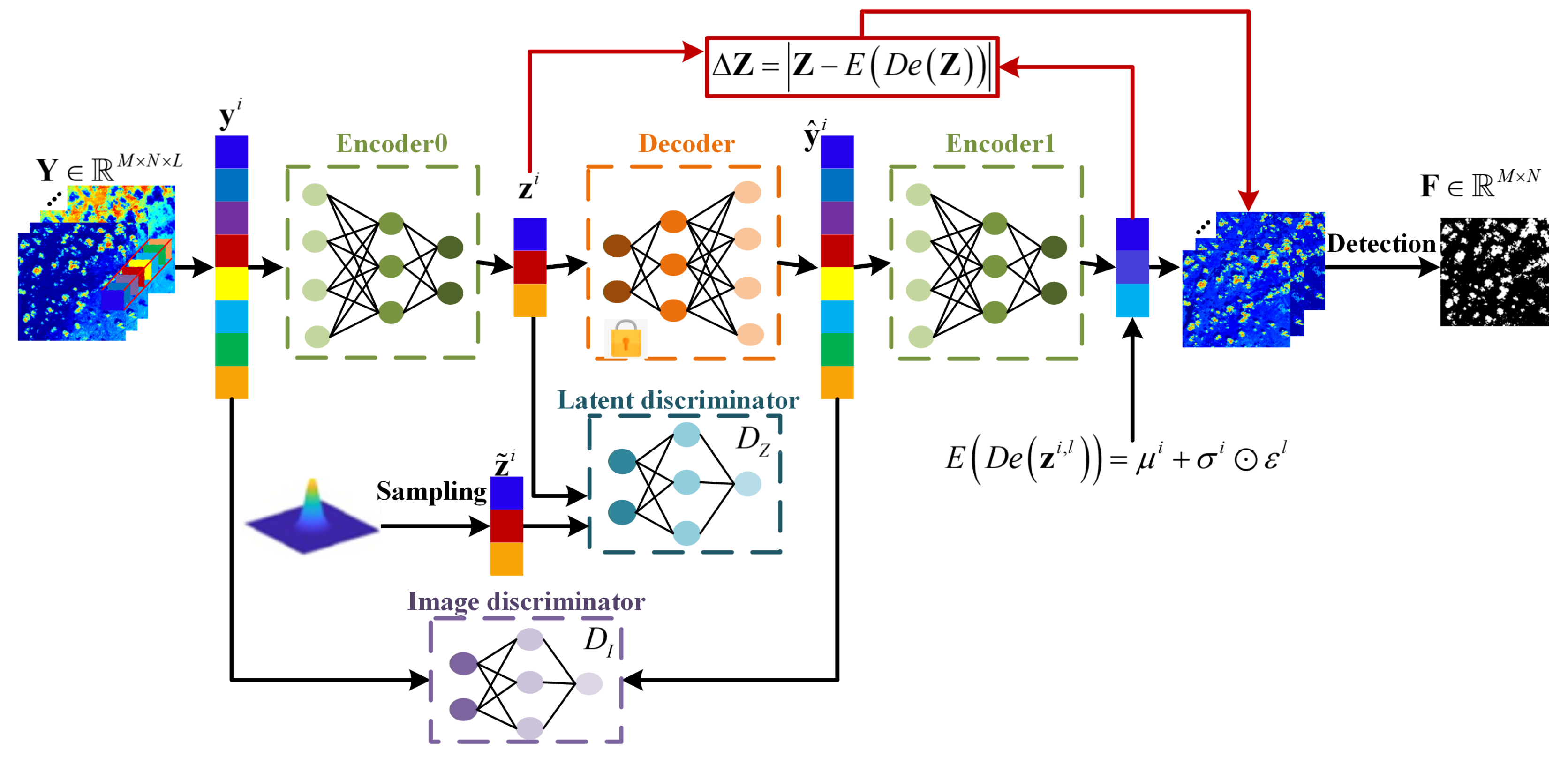
  • A multivariate Gaussian distribution is adopted to extract a discriminative feature matrix of the background in the latent space, and the residual error between the low-dimensional representations of the original and background pixels is beneficial to cloud detection.
The remainder of this paper is organized as follows. In Section 2, AE and adversarial learning models are briefly described. Section 3 introduces the proposed UNCD framework. The experimental results and discussion are presented in Section 4. The discussion of the experimental results is introduced in Section 5. Finally, Section 6 presents the conclusions of this study.

2. Related Work

2.1. Generative Adversarial Network

A generative adversarial network (GAN) is a highly efficient generation model proposed by Goodfellow et al. [33] in 2014. GANs consist of a generator G and a discriminator D, which are trained against each other. The generator G inputs a random data z whose probability distribution is p z z and outputs a data x f a k e = G ( z ) . The discriminator D receives two inputs, real data x with a probability distribution p d a t a x and generated data G ( z ) . The discriminator is trained to identify the real data. Via successive adversarial learning, G generates increasingly many real data. The objective of this adversarial learning process can be expressed as [33]:
min G max D E x p d a t a x log D x + E z p z z log 1 D G z .
Due to its advantages in terms of generation and adversarial learning performance, we constructed a GAN model that is based on an encoder and a decoder for the improved production of discriminative features.

2.2. Variational Autoencoders
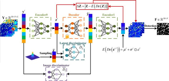
An AE updates the parameters by minimizing the distance between the input data and the reconstructed data, which is an unsupervised neural network. Many extensions that are based on AEs have been proposed and broadly used, one of which is the variational AE (VAE) [32]. The VAE conducts variational inference to match the distribution of the hidden code vector of the AE with a predefined prior distribution. From the perspective of the probabilistic graph model, the encoder and decoder of the VAE can be interpreted as a probabilistic encoder and a probabilistic decoder, which are denoted as p θ ( x | z ) and q ϕ ( z | x ) , respectively [32]. To match the distribution of the hidden code vector z with a predefined prior distribution, variational inference is performed to optimize the variational lower bound on the marginal log-likelihood of each observation. Thus, the objective function of VAE can be expressed as:
v a e = K L q ϕ z x i p θ z + E q ϕ z x i log p θ x i z ,
where x i refers to a sample from the training dataset. The first term is the KL-divergence term, which represents the difference between the distribution of the extracted latent feature samples and the Gaussian distribution. The smaller the difference, the closer the distribution of the extracted latent features is to the Gaussian distribution. The second term is the AE’s reconstruction error, which represents the expectation of the reconstruction error, namely, the gap between the input and the output. The smaller the expected value of the reconstruction error, the closer the output can be to the input. The hidden code vector z is sampled from z i , l = μ i + σ i ε l , where ε l N 0 , I . Both the encoder and the decoder originally leverage the sigmoid function as the nonlinear activation function. Recently, the rectified linear unit (ReLU) [34] has been widely used as the nonlinear activation function.

3. Proposed Method

Figure 1 illustrates the overall framework of our proposed UNCD method. Let Y = y i i = 1 M × N , y i R L × 1 denote an input remote sensing image with M × N spectral vectors, and each spectral vector contains L dimensions. Firstly, the underlying characteristics are extracted by an encoder E and a decoder D e trained via an adversarial approach, thereby yielding a compact representation Z = z i i = 1 M × N , z i R l × 1 , l < L of the redundant remote sensing images. Based on the observation that clouds are sparse and modeled as sparse outliers, some powerful constraints are imposed on the unsupervised neural network for the extraction of a discriminative feature matrix E D e Z of the background, which has the same dimension as Z . Due to the reconstruction ability of AEs and the generation capability of GANs, it is possible to obtain features of the full image and the background in deep latent space, respectively. As a consequence, Z and E D e Z are compact representations of the original image and background, respectively. Specifically, the residual error between Z and E D e Z is beneficial to cloud detection. More details of each step are described as follows.

3.1. Constructing the Residual Error in the Latent Space

The proposed UNCD method relies on two assumptions for cloud detection. One is that the background can be distinguished from the clouds in the latent feature space and most of a remote sensing scene is background, while clouds are sparse. When a remote sensing image Y that contains clouds is input into the network, the network is expected to generate a compact representation of Y and to reconstruct a corresponding background via an unsupervised approach. Consequently, the residual error refers to the deep latent feature space in which the clouds are enhanced, and the background is suppressed:
Δ Z = Z E D e Z .
The encoder learns a mapping from input Y into the deep latent space, which produces a feature matrix Z that preserves the essential information including the clouds and background. Then, Z is input into the decoder D e to reconstruct Y . Since sufficient training samples are available for most of the background and clouds are sparse with limited training samples in a remote sensing scene, the decoder produces small reconstruction error for the background region but relatively large reconstruction error for the clouds. The adversarial leaning terms and physical constraints regarding the characteristics of the cloud-contaminated images are imposed on the network to enhance the capability of discriminative feature learning performance.

3.2. Adversarial Feature Learning Term

Adversarial feature learning is used in the latent space to extract distinctive features. As shown in Figure 1, the encoder0 acts as a generator to produce latent feature variables z i q E 0 y i , which strives to fool the latent discriminator D z with z i p z i sampled from the prior distribution. The latent discriminator D z aims to distinguish between input that comes from the encoder z i q E 0 y i versus that from prior distribution z i p z i . As a consequence, the generator (encoder) E 0 attempts to minimize this objective against the latent discriminator D z that attempts to solve min E 0 max D z L o s s a d v _ z , where L o s s a d v _ z is denoted as:
L o s s a d v _ z = E z i N 0 , I log D z z i + E z i q E 0 y i log 1 D z E 0 y i .
Here, we set the prior distribution z i p z i as multivariate Gaussian distribution to extract feature variables that are more beneficial to cloud detection considering that clouds are sparse and the majority is background.

3.3. Adversarial Image Learning Term

The adversarial feature learning in the previous part may generate out-of-class features due to the capability of GAN to generate new variants. To generate features of the original remote sensing images, we constrain the network by the image discriminator D I to avoid the generation of out-of-class features, as illustrated in Figure 1. Via this approach, the decoder D e and the image discriminator D I are combined into a GAN again, in the training phase of which the decoder D e is changed to a generator to ensure that the generated image can fool the image discriminator D I . The image discriminator D I aims to distinguish whether its input comes from the generator D e or the real input. The optimization problem is to achieve min D e max D I L o s s a d v _ I , where L o s s a d v _ I can be expressed as:
L o s s a d v _ I = E y i p d a t a log D I y i + E z i N 0 , I log 1 D I D e z i .
The first term indicates that the discriminator attempts to maximize the output of the real sample to make it closer to 1. The second term indicates that by optimizing the discriminator, the output to the generated sample becomes closer to zero. At the same time, the generator is optimized, thereby making the output of the discriminator on the generated samples closer to 1.

3.4. Latent Representation of the Background

The Gaussian distribution that is imposed on the network focuses on reconstructing the majority class, namely, the background, with relatively sufficient samples. Consequently, the generated image D e Z with the same size as the input is closer to the background than to the clouds. Due to the strong representational capability of AE, it can still reconstruct the sparse pixels (i.e., the clouds). To further reduce the proportion of clouds in the reconstructed image D e Z , we impose the representation consistency constraint in the deep latent feature space, that is, we enforce the satisfaction of a multivariate Gaussian distribution by E D e Z via an unsupervised approach that better accords with the background characteristics:
L o s s G a u s s = K L q E D e z i D e z i p E D e z i ,
where E D e z i , l = μ i + σ i ε l and ε l N 0 , I . The encoded output of the second encoder is represented by E D e z i , and the output of the first decoder is denoted by D e z i . During the training of encoder1, only the parameters of the encoder are optimized, while the parameters of the decoder D e are kept fixed as, illustrated in Figure 1. E D e z i , l is the projection of the reconstructed spectral vector D e z i in the low-dimensional latent space, which is the enhanced background representation obtained by imposing the representation consistency constraint. Thus, the distinctive residual error for distinguishing between the background and the clouds in the low-dimensional latent space can be calculated via Equation (3), and an example is represented in Figure 2.

3.5. Reconstruction Loss

In a traditional AE network, the input data are encoded by the hidden layers to be decoded correctly in the output. The parameters are selected such that the objective of minimizing the following cost function is realized:
L o s s r = y i y ^ i 2 ,
where y i denotes an input spectral vector with L dimensions and y ^ i denotes the corresponding reconstructed spectral vector. Finally, the combination of the aforementioned losses yields
L o s s = L o s s a d v _ z + L o s s a d v _ I + L o s s G a u s s + L o s s r .
The model is trained and updated via the stochastic gradient descent (SGD) algorithm. When the model loss converges, the parameters, including the weight matrix and the bias, are obtained. According to Figure 2, the compact representation of the original image, Z , contains features of both clouds and background regions, whereas E D e Z can well represent the background information with the clouds restricted. As a consequence, the residual error Δ Z obtained from the pixel-wise difference enhances the clouds while suppressing the background in the lower-dimensional feature space, which facilitates the detection of clouds as shown in Figure 3. Subsequently, an adaptive weighting method that was proposed in our previous work [35,36] is applied on each dimension of the residual error Δ Z to discard redundant information and to construct a comprehensive map, where the structure tensor (ST) is utilized. The ST of the ith dimension in the residual error Δ Z can be defined as [35,36]:
S i = Δ Z i x 2 Δ Z i x Δ Z i y Δ Z i x Δ Z i y Δ Z i y 2 ,
where Δ Z i x = Δ Z i x and Δ Z i y = Δ Z i y represent the derivatives of the ith dimension of the residual error Δ Z along the x and y directions, respectively. Since this structure tensor S i of the ith dimension is a semi-determined matrix, it can be decomposed into [35,36]:
S i = η 1 i η 2 i λ 1 i 0 0 λ 2 i η 1 i η 2 i ,
where λ 1 i and λ 2 i are the non-negative eigenvalues of the ith dimension and η 1 i , η 2 i are the corresponding eigenvectors. The larger eigenvalue is represented by λ 1 i . As discussed in our previous work [35,36], the relative larger eigenvalue can represent the response intensity of each pixel in the corresponding dimension of Δ Z . Therefore, the weight vector for each dimension of Δ Z is calculated from the relative larger eigenvalue. The larger the edge intensity of the ith dimension, the more structural information the ith dimension of Δ Z contains. Consequently, the ith dimension should occupy a larger proportion. The ( i 1 ) th dimension should also occupy a larger proportion. If the larger eigenvalues of all the dimensions are same, all the dimensions will have the same proportion, which is the same as the result obtained with the averaging function. In summary, the weighted residual error Δ Z ^ is calculated as [35,36]:
Δ Z ^ = i = 1 l λ 1 i i = 1 l λ 1 i Δ Z i ,
where l is the dimension of Δ Z . To further consider that the adjacent pixels have high correlations with each other, we utilize a guided filter [37] to move the neighboring pixels to the same object for both the background and clouds. Finally, we use an iterative optimization step to further increase the detection accuracy, namely, we multiply the initial detection map by the residual error Δ Z , and repeat the detection procedure until the following stopping rule is satisfied:
C D f 1 C D f 10 4 ,
where C D f 1 and C D f represent the ( f 1 ) th and fth detection maps, respectively. According to this stopping rule, if the ( f 1 ) th and fth detection maps are highly similar, the iterative optimization will terminate.

3.6. Data Description

3.6.1. Landsat 8 Dataset

The Landsat 8 dataset was made available online https://www.usgs.gov/land-resources/nli/landsat/spatial-procedures-automated-removal-cloud-and-shadow-sparcs-validation, and is widely used to evaluate the cloud detection methods due to its wide coverage and high resolution. This dataset consists of 80 MS remote sensing images, with details described in [38]. The Landsat 8 dataset was collected globally using two instruments: OLI (Operational Land Imager) and TIRS (Thermal Infrared Sensor). We use the data from both of these. All the channels are used for cloud detection. The spatial resolution of each Landsat image is 30 m—that is, each pixel represents information on an area of 900 m 2 . The location of the dataset is global. Each image contains 1000 × 1000 pixels in the spatial domain and ten bands in the spectral domain. The corresponding reference maps are shown in Figure 4.

3.6.2. GF-1 WFV Dataset

The GaoFen-1 (GF-1) satellite was launched by China. Gaofen means “high resolution” in Chinese. Detailed information on the GF-1 satellite and wide field of view (WFV) images are available online http://sendimage.whu.edu.cn/en/resources/mfc-validation-data/. The GF-1 WFV image considered here is a Class 2A product produced via relative radiation correction and system geometry correction. The Class 1A data are the original digital product for regular radiation calibration, while the Class 2A data were generated after system geometry correction, where all pixels are re-sampled to 16-m resolution with 10-bit data. The false-color images and the corresponding reference maps are shown in Figure 5.

3.6.3. GF-5 Hyperspectral Dataset

The GaoFen-5 (GF-5) satellite can capture hyperspectral observations in the Chinese Key Projects of the High-Resolution Earth Observation System. Six payloads were carried on it: an Advanced Hyperspectral Imager (AHSI), a Visual and Infrared Multispectral Imager (VIMI), an Atmospheric Infrared Ultra-Spectral Sounder (AIUS), a Greenhouse Gases Monitoring Instrument (GMI), an Environmental Monitoring Instrument (EMI), and a Directional Polarization Camera (DPC). The spectral coverage of these sensors ranges from ultraviolet to long-wave infrared bands. Two HS images captured by the GF-5 AHSI sensor were used to evaluate the performance of the proposed method. Each image has a size of 430 × 430 × 180 pixels. The false-color images are shown in Figure 6. The reference maps for this dataset have not been published yet.

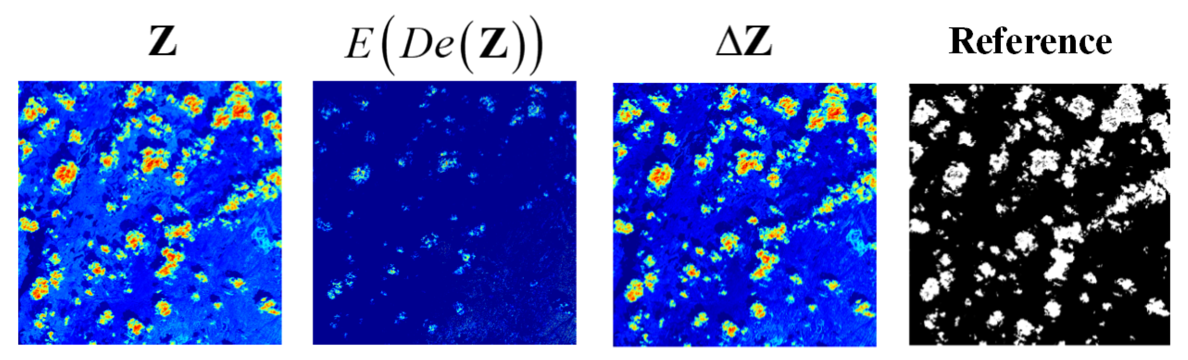
4. Experimental Results

We comprehensively evaluated the proposed method on three real datasets, which included MS and HS images captured by various imaging sensors over various scenes. First, we describe the dataset. Then, we introduce the compared methods and evaluation criterion. Third, we further investigate the performance of the proposed UNCD method, both qualitatively and quantitatively. Finally, we analyze the impact of the network structure on the detection performance.

4.1. Experimental Setting

Due to insufficient samples in the remote sensing imagery, we fixed the depth of our UNCD to 2 to avoid overfitting. Inspired by [39], the number of hidden nodes was fixed to L + 1 , where L is the number of bands of the input remote sensing image. The leaky ReLU (LReLU) was used as the nonlinear activation function with a slope of 0.2 to compress the negative input and retain the negative part of the information to a certain extent. As the number of epochs increases, both the detection performance and the computational complexity increase. Thus, we set the number of epochs to 1000 as a trade-off. The batch size was fixed to the number of pixels in the spatial domain, namely, M × N for each remote sensing image. The learning rate was set to 0.01. The parameters introduced above were set to the default values in our experiments, and they can be tuned by the user for the optimal results.
We conducted experiments on 8 NVIDIA Tesla k80 graphics cards based on a system running Python 3.6.0 and TensorFlow 1.10.0. All compared methods were implemented in MATLAB R2017a.

4.2. Compared Methods and Evaluation Criterion

To evaluate the performance of the proposed UNCD model, several representative cloud detection methods that are frequently cited in the literature, namely, K-means, PRS, SVM, PCANet, and SL, were employed for comparison in terms of both visual effects and quantitative evaluations. The K-means method is a typical unsupervised method. The PRS method yields satisfactory results on several remote sensing images, and is also an unsupervised method. Since the PRS method is only applicable to RGB images, we combined band 4-red, band 3-green, and band 2-blue into RGB images. The SVM, PCANet, and SL methods are supervised learning methods for cloud detection.
To comprehensively evaluate the cloud detection results, the three commonly used evaluation criteria, namely, the area under the curve (AUC) [40] of the receiver operating characteristic (ROC), the overall accuracy (OA), and the kappa coefficient (Kappa), were employed.
The area under the curve (AUC) [40] is widely used in objective evaluation indices. The AUC can identify general trends in the detection performance. The larger the AUC value of the ROC curve, the better the performance. The OA is defined as [41]:
OA = TP + TN TP + TN + FN + FP ,
where true positives (TPs), true negatives (TNs), false positives (FPs) and false negatives (FNs) represent the number of correctly detected cloud pixels, the number of correctly detected non-cloud pixels, the number of false-alarm pixels, and the number of missed cloud pixels, respectively. The kappa coefficient reflects the agreement between a final cloud detection image and the ground-truth map. Compared with the overall accuracy (OA), the kappa coefficients can more objectively reflect the accuracy of the results. The larger the value of the kappa coefficient, the higher the accuracy of the result will be. The kappa coefficient is calculated as [41]:
Kappa = OA P 1 P ,
where
P = ( TP + FP ) ( TP + FN ) ( TP + FP + FN + TN ) 2 + ( FN + TN ) ( FP + TN ) ( TP + FP + FN + TN ) 2 .

4.3. Cloud Detection Results

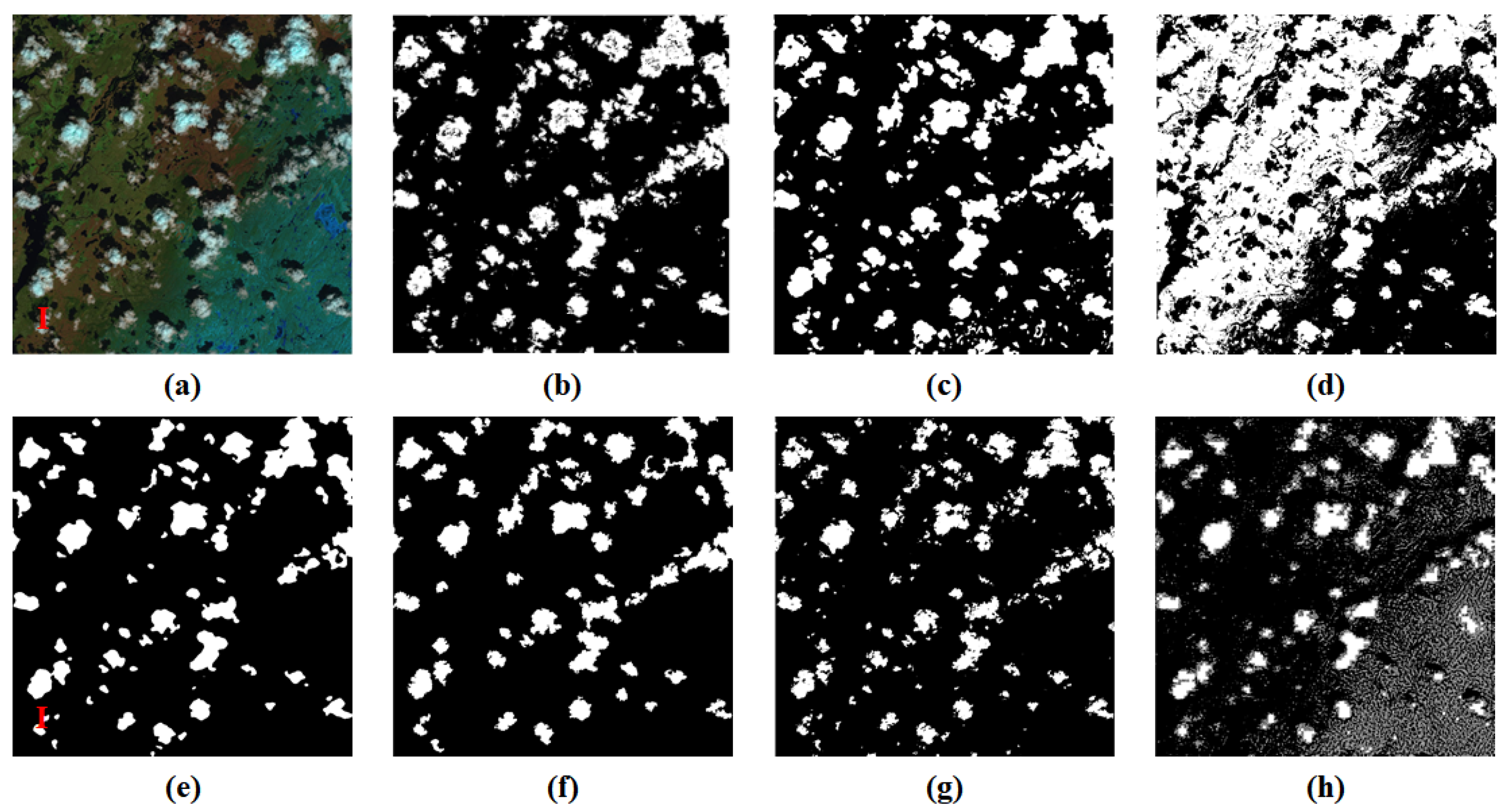
4.3.1. Landsat 8 Dataset Results

The reference maps and the visual cloud detection results that were obtained by the competing methods for two images from the Landsat 8 dataset are shown in Figure 4 and Figure 5. The reference map is published at the same time as the dataset and used together with the data. Moreover, the provider of the dataset marks the annotation. Image I is an example of a case with thin clouds, and Image II is an example of a case with thick clouds. With these two images, we compared our method with K-means, PRS, SVM, PCANet, and SL. We implemented these compared methods via the publicly released codes. According to Figure 4 and Figure 5, the proposed UNCD method caused the smallest visual difference between the reference map and the detection map compared to K-means, PRS, SVM, PCANet, and SL. As illustrated in Figure 4 and Figure 5, the K-means method yielded many noise-like detection results. The PRS method realized minimal improvement for Image I with respect to the K-means method, and thin clouds were undetected in large areas in Image I. The SL method generated some detection mistakes in the image due to the thinness and thickness of the clouds. The PCANet and SVM methods outperformed the K-means, PRS, and SL methods. In particular, the proposed UNCD method could accurately distinguish clouds and complex background scenes. The reason is that the proposed detection method extracts the spectral features of the image while utilizing the spatial background information between adjacent pixels. In comparison to these methods, the advantage of the proposed UNCD method is its robust detection performances for different clouds with different scales in different scenes. The objective evaluations, including AUC, OA, and Kappa obtained by all the considered algorithms, are reported in Table 1, which complies with the visual observation. Concretely, the AUCs obtained by the proposed UNCD method were 0.9543 and 0.9637 for Images I and II, respectively, which are much higher than those obtained by the second-best approach in each case, 0.8485 (PRS method) and 0.8848 (K-means method). The OA and Kappa obtained by the proposed UNCD method were also the highest, and much higher than those obtained by the second-best method.

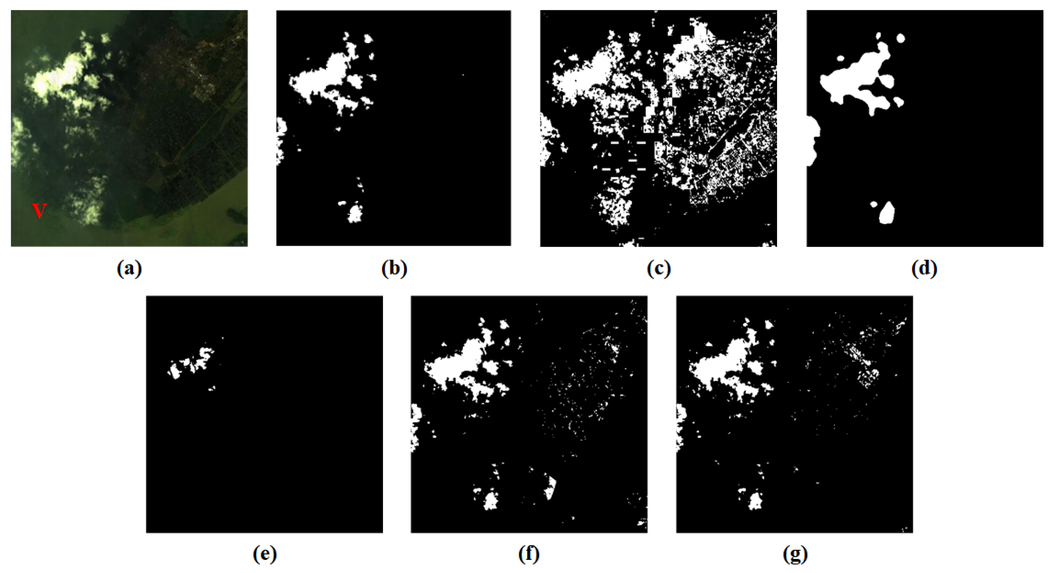
4.3.2. GF-1 WFV Dataset

The reference maps and detection maps obtained by the compared methods are shown in Figure 6 and Figure 7. The detection results obtained by the proposed method were similar to the reference maps, indicating that the proposed method could obtain a satisfactory detection performance. It is apparent that the UNCD method achieved better detection results than the K-means, PRS, PCANet, SVM, and SL methods. For the GF-1 WFV dataset, Table 2 lists the corresponding quantitative metrics. In addition, the competing methods are also reported in Table 2. From Table 2, the AUC values, OA, and Kappa obtained by the proposed UNCD method were the best among the compared methods. The reported OA scores on Images III and IV (0.9957 and 0.9934) obtained by the proposed UNCD method were higher than that obtained by the second-best methods (0.9835 for SVM on Image III and 0.9690 for SL on Image IV).

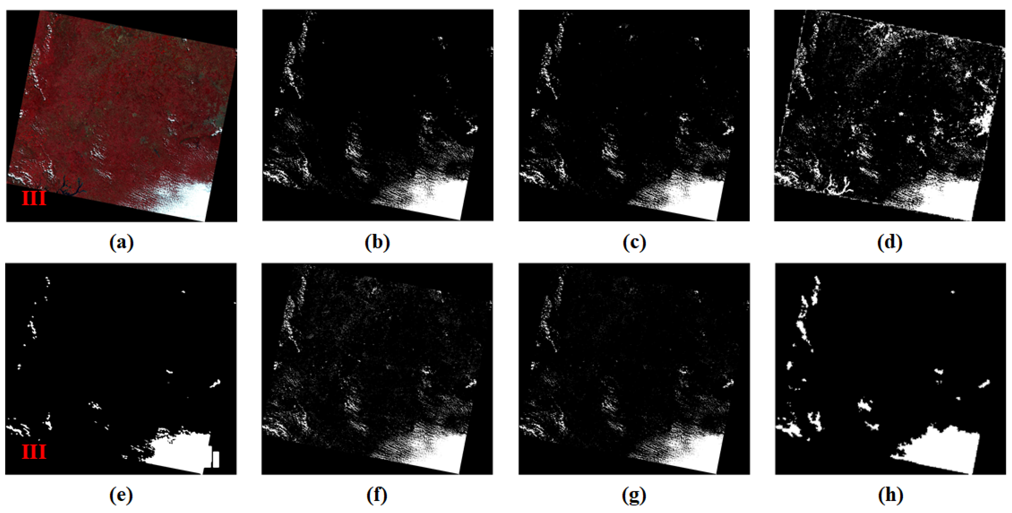
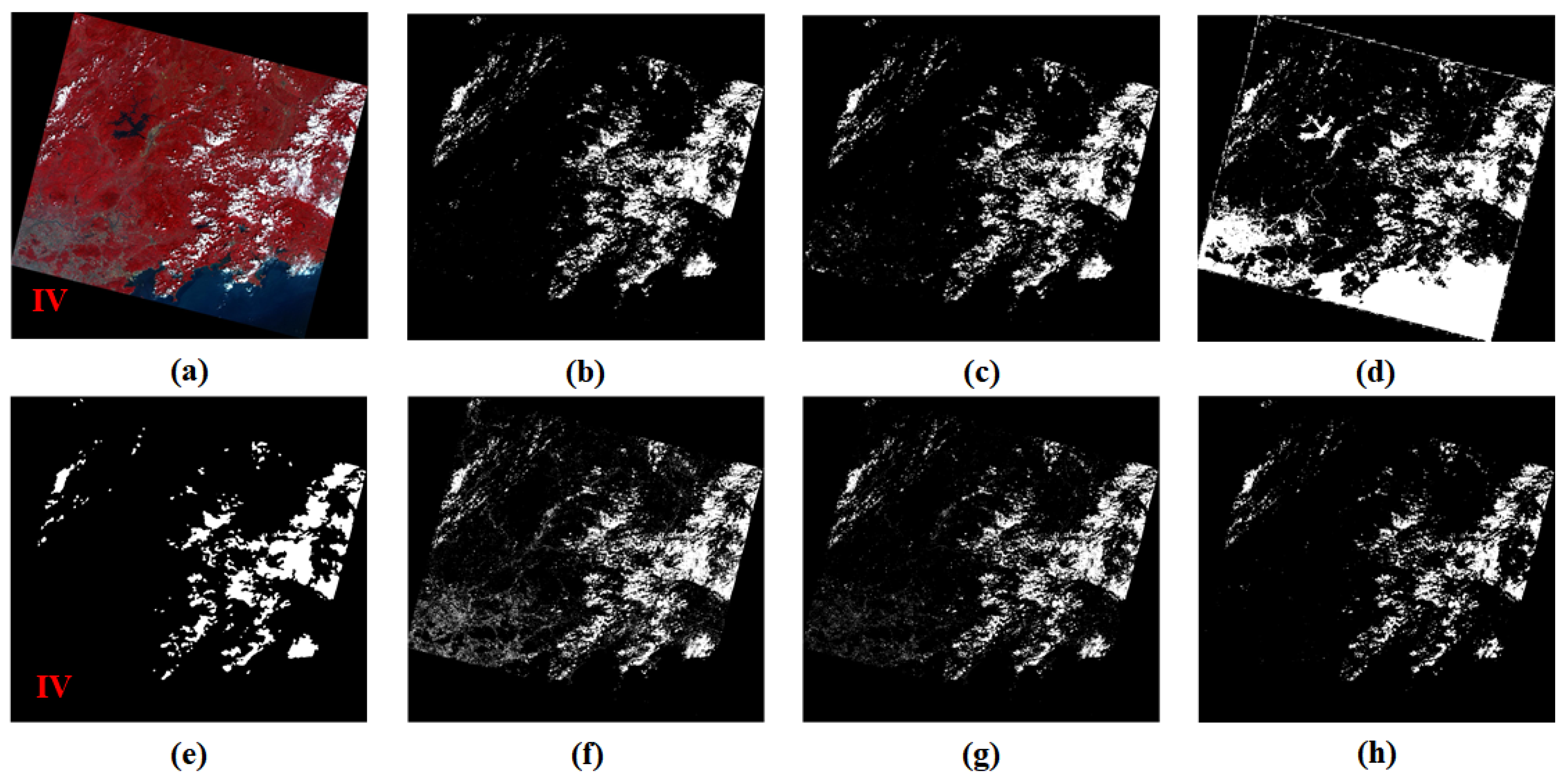
4.3.3. GF-5 Hyperspectral Dataset

The GF-5 dataset was used to evaluate the feasibility of our proposed UNCD method on real hyperspectral data. The cloud detection results are displayed in Figure 8 and Figure 9. Image V in Figure 8 contains large clouds, while Image VI in Figure 9 contains many small clouds. It can be observed that our method was capable of discriminating clouds of different sizes from the background pixels. The K-means method introduced many false positives. PRS and PCANet failed to detect all the clouds. By contrast, the SVM and SL methods had better performance while also generating some detection mistakes. For example, the buildings in Image V were still detected as clouds by the SVM and SL methods.

4.4. Component Analysis

This section analyzes the effects of the significant processing components on the detection performance on each dataset. Since the reference maps of the GF-5 hyperspectral dataset are not publicly available, the objective evaluations could not be obtained for this dataset. Therefore, four remote sensing images coming from the Landsat 8 dataset and the GF-1 WFV dataset were used to evaluate the effect of each component objectively. Three comparison experiments were conducted. In the first experiment, only the AE was considered, which is a basic model for joint encoder–decoder training. The second considered AE with additional adversarial training (a latent feature discriminator). The third utilized the proposed method. The AUC, OA, and Kappa values were calculated as reported in Table 3. The better the detection performance, the higher the AUC, OA, and Kappa values. The AUC values were 0.9254, 0.9025, 0.9436, and 0.9462 for four images when only using AE. When applying the adversarial feature learning, the AUC values were improved to 0.9477, 0.9379, 0.9506, and 0.9689, respectively. When the multivariate Gaussian distribution was introduced, the method yielded the best AUC values, which reached 0.9543, 0.9637, 0.9676, and 0.9860, respectively. Similarly, the other two indicators (i.e., OA and Kappa) also increased. These results demonstrate that each component of the proposed UNCD method has a positive influence on the cloud detection performance.

5. Discussion

According to the values of AUC, OA, and Kappa in Table 1 and Table 2 and the visual observations in Figure 4, Figure 5, Figure 6, Figure 7, Figure 8 and Figure 9 for various types of datasets, compared to several state-of-the-art methods, the proposed UNCD method performed the best in detection according to both the objective evaluation results and the visual observations. The superior performance of the proposed method is due to the latent adversarial learning constrained encoder, the image discriminator, and the multivariate Gaussian distribution in the network architecture. It can be concluded from the component analysis experiments that each part had a positive impact on the detection results. While the proposed UNCD method yielded promising results in cloud detection, several areas were identified during experiments for improvement in future work. It is worthwhile to further utilize the data characteristics of remote sensing images in order to optimize unsupervised networks and to improve the cloud detection performance. In addition, the network architecture can be enhanced by adding some loss functions and constraints.
The OA values of Images I–IV that were obtained by the proposed UNCD method were 0.9526, 0.9536, 0.9957, and 0.9934, respectively. Our method outperformed the second-best method by 1.44%, 5.23%, 1.24%, and 1.96%, respectively. While the performance of our method was the best among the considered methods, there is still room for improvement. Moreover, the accuracy of cloud detection was not high, and there were still many missed detections. However, other comparison methods also have this problem. Meanwhile, the proposed UNCD method is devoted to cloud detection. In the future, we will further realize cloud shadow detection. At the same time, to make the method universal, we will conduct additional experiments on datasets acquired by additional sensors.

6. Conclusions

In this paper, we proposed a discriminative feature learning constrained unsupervised network for cloud detection (UNCD) for remote sensing imagery. The induced latent discriminator, image discriminator, and multivariate Gaussian distribution consider the fact that clouds are sparse and modeled as outliers and realize a discriminative residual map between the original input and the background. Based on the analysis of the strong correlation between adjacent pixels, a guided filter is employed on the residual map to obtain an initial detection map. To further improve the detection performance, an iterative optimization algorithm is introduced which terminates automatically if the stopping condition is satisfied. Extensive experimental results on several datasets demonstrate that the proposed UNCD not only realizes a more favorable detection performance but also generalizes better to different datasets compared with other state-of-the-art methods. Moreover, the OA values for Images III and IV from the GF-1WFV dataset were 0.9957 and 0.9934, respectively. This signifies that our algorithm performwe better than other known algorithms. In future work, we will expand the datasets used for the experiments to improve the performance of the algorithm.

Author Contributions

W.X. conceived and designed the study; J.Y. and J.L. (Jie Lei) performed the experiments and analyzed the result data; W.X. and Y.L. investigated related work; J.Z. and J.L. (Jiaojiao Li) reviewed and edited the manuscript; W.X. wrote the paper. All authors read and approved the manuscript.

Funding

This work was supported in part by the National Natural Science Foundation of China under Grant 61801359, Grant 61571345, Grant 91538101, Grant 61501346, Grant 61502367, and Grant 61701360, in part by the Young Talent fund of University Association for Science and Technology in Shaanxi of China under Grant 20190103, in part by the Special Financial Grant from the China Postdoctoral Science Foundation under Grant 2019T120878, in part by the 111 project under Grant B08038, in part by the joint fund project of NSFC under Grant U1704130, in part by the Fundamental Research Funds for the Central Universities under Grant JB180104, in part by the Natural Science Basic Research Plan in Shaanxi Province of China under Grant 2019JQ153, Grant 2016JQ6023, and Grant 2016JQ6018, in part by the General Financial Grant from the China Postdoctoral Science Foundation under Grant 2017M620440, in part by the Yangtse Rive Scholar Bonus Schemes under Grant CJT160102, and in part by the Ten Thousand Talent Program.

Conflicts of Interest

The authors declare no conflicts of interest.

Abbreviations

The following abbreviations are used in this manuscript:
AHSIAdvanced Hyperspectral Imager
AIUSAtmospheric Infrared Ultra-spectral Sounder
AUCArea under the curve
CDnetCloud detection neural network
CNNConvolutional neural network
DNNDeep neural network
DPCDirectional Polarization Camera
EMIEnvironmental Monitoring Instrument
FNFalse negative
FPFalse positive
GANGenerative adversarial network
GF-1GaoFen-1
GF-5GaoFen-5
GMIGreenhouse Gases Monitoring Instrument
HRGHigh-resolution geometric
HSHyperspectral
KappaKappa coefficient
MSMultispectral
MSCFFMultiscale convolutional feature fusion
OAOverall accuracy
OLIOperational Land Imager
PCANetPrincipal component analysis network
PRSProgressive refinement scheme
ROCReceiver operating characteristic
SGDStochastic gradient descent
SLScene learning
STStructure tensor
SVMSupport vector machine
TPTrue positive
TNTrue negative
TIRSThermal Infrared Sensor
UNCDunsupervised network for cloud detection
VAEVariational autoencoder
VIMIVisual and Infrared Multispectral Imager
WFVWide field of view

References

  1. Lei, J.; Xie, W.; Yang, J.; Li, Y.; Chang, C.I. Spectral-spatial feature extraction for hyperspectral anomaly detection. IEEE Trans. Geosci. Remote Sens. 2019, 57, 8131–8143. [Google Scholar] [CrossRef]
  2. Xie, W.; Shi, Y.; Li, Y.; Jia, X.; Lei, J. High-quality spectral-spatial reconstruction using saliency detection and deep feature enhancement. Pattern Recognit. 2019, 88, 139–152. [Google Scholar] [CrossRef]
  3. Jiang, T.; Li, Y.; Xie, W.; Du, Q. Discriminative reconstruction constrained generative adversarial network for hyperspectral anomaly detection. IEEE Trans. Geosci. Remote Sens. 2020. to be published. [Google Scholar] [CrossRef]
  4. Nasrabadi, N.M. Hyperspectral target detection: An overview of current and future challenges. IEEE Signal Process. Mag. 2014, 31, 34–44. [Google Scholar] [CrossRef]
  5. Yuan, Y.; Ma, D.; Wang, Q. Hyperspectral anomaly detection by graph pixel selection. IEEE Trans. Cybern. 2016, 46, 3123–3134. [Google Scholar] [CrossRef]
  6. Li, Y.; Xie, W.; Li, H. Hyperspectral image reconstruction by deep convolutional neural network for classification. Pattern Recognit. 2017, 63, 371–383. [Google Scholar] [CrossRef]
  7. Zhang, Y.; Rossow, W.B.; Lacis, A.A.; Oinas, V.; Mishchenko, M.I. Calculation of radiative fluxes from the surface to top of atmosphere based on ISCCP and other global data sets: Refinements of the radiative transfer model and the input data. J. Geophys. Res. Atmos. 2004, 109, D19105. [Google Scholar] [CrossRef] [Green Version]
  8. Xie, W.; Li, Y.; Zhou, W.; Zheng, Y. Efficient coarse-to-fine spectral rectification for hyperspectral image. Neurocomputing 2018, 275, 2490–2504. [Google Scholar] [CrossRef]
  9. Fisher, A. Cloud and cloud-shadow detection in SPOT5 HRG imagery with automated morphological feature extraction. Remote Sens. 2014, 6, 776–800. [Google Scholar] [CrossRef] [Green Version]
  10. Zhang, Q.; Xiao, C. Cloud detection of RGB color aerial photographs by progressive refinement scheme. IEEE Trans. Geosci. Remote Sens. 2014, 52, 7264–7275. [Google Scholar] [CrossRef] [Green Version]
  11. Li, Z.; Shen, H.; Li, H.; Xia, G.; Gamba, P.; Zhang, L. Multi-feature combined cloud and cloud shadow detection in GaoFen-1 wide field of view imagery. Remote Sens. Environ. 2017, 191, 342–358. [Google Scholar] [CrossRef] [Green Version]
  12. Zhong, B.; Chen, W.; Wu, S.; Hu, L.; Luo, X.; Liu, Q. A cloud detection method based on relationship between objects of cloud and cloud-shadow for Chinese moderate to high resolution satellite imagery. IEEE J. Sel. Top. Appl.Earth Observat. Remote Sens. 2017, 10, 4898–4908. [Google Scholar] [CrossRef]
  13. Ishida, H.; Oishi, Y.; Morite, K.; Moriwaki, K.; Nakajima, T.Y. Development of a support vector machine based cloud detection method for MODIS with the adjustability to various conditions. Remote Sens. Environ. 2018, 205, 309–407. [Google Scholar] [CrossRef]
  14. An, Z.; Shi, Z. Scene learning for cloud detection on remote-sensing images. IEEE J. Sel. Top. Appl.Earth Observat. Remote Sens. 2015, 8, 4206–4222. [Google Scholar] [CrossRef]
  15. Li, P.; Dong, L.; Xiao, H.; Xu, M. A cloud image detection method based on SVM vector machine. Neurocomputing 2015, 169, 34–42. [Google Scholar] [CrossRef]
  16. Kanungo, T.; Mount, D.M.; Netanyahu, N.S.; Piatko, C.D.; Silverman, R.; Wu, A.Y. An efficient K-means clustering algorithm: Analysis and implementation. IEEE Trans. Pattern Anal. Mach. Intell. 2002, 24, 881–892. [Google Scholar] [CrossRef]
  17. Xie, W.; Jia, X.; Li, Y.; Lei, J. Hyperspectral image super-resolution using deep feature matrix factorization. IEEE Trans. Geosci. Remote Sens. 2019. to be published. [Google Scholar] [CrossRef]
  18. Wu, H.; Prasad, S. Semi-supervised deep learning using pseudo labels for hyperspectral image classification. IEEE Trans. Image Process. 2018, 27, 1259–1270. [Google Scholar] [CrossRef]
  19. Xie, W.; Li, L.; Hu, J.; Chen, D.Y. Trainable spectral difference learning with spatial starting for hyperspectral image denoising. IEEE Trans. Image Process. 2018, 108, 272–286. [Google Scholar] [CrossRef]
  20. Ienco, D.; Pensa, R.G.; Meo, R. A semisupervised approach to the detection and characterization of outliers in categorical data. IEEE Trans. Neural Netw. Learn. Syst. 2017, 28, 1017–1029. [Google Scholar] [CrossRef] [Green Version]
  21. Shi, M.; Xie, F.; Zi, Y.; Yin, J. Cloud detection of remote sensing images by deep learning. In Proceedings of the IEEE International Geoscience and Remote Sensing Symposium (IGARSS), Beijing, China, 10–15 July 2016; pp. 701–704. [Google Scholar]
  22. Goff, M.L.; Tourneret, J.Y.; Wendt, H.; Ortner, M.; Spigai, M. Deep learning for cloud detection. In Proceedings of the International Conference of Pattern Recognition Systems(ICPRS), Fort Worth, TX, USA, 23–28 July 2017; pp. 1–6. [Google Scholar]
  23. Ozkan, S.; Efendioglu, M.; Demirpolat, C. Cloud detection from rgb color remote sensing images with deep pyramid networks. arXiv 2018, arXiv:cs.CV/1801.08706. [Google Scholar]
  24. Zi, Y.; Xie, F.; Jiang, Z. A cloud detection method for Landsat 8 images based on PCANet. Remote Sens. 2018, 10, 877. [Google Scholar] [CrossRef] [Green Version]
  25. Shao, Z.; Pan, Y.; Diao, C.; Cai, J. Cloud detection in remote sensing images based on multiscale features-convolutional neural network. IEEE Trans. Geosci. Remote Sens. 2019, 57, 4062–4076. [Google Scholar] [CrossRef]
  26. Yang, J.; Guo, J.; Yue, H.; Liu, Z.; Hu, H.; Li, K. CDnet: CNN-based cloud detection for remote sensing imagery. IEEE Trans. Geosci. Remote Sens. 2019. to be published. [Google Scholar] [CrossRef]
  27. Li, Z.; Shen, H.; Cheng, Q.; Liu, Y.; You, S.; He, Z. Deep learning based cloud detection for medium and high resolution remote sensing images of different sensors. ISPRS J. Photogramm. Remote. Sens. 2019, 150, 197–212. [Google Scholar] [CrossRef] [Green Version]
  28. Zhang, Y.; Wen, F.; Gao, Z.; Ling, X. A coarse-to-fine framework for cloud removal in remote sensing image sequence. IEEE Trans. Geosci. Remote Sens. 2019. to be published. [Google Scholar] [CrossRef]
  29. Wen, F.; Zhang, Y.; Gao, Z.; Ling, X. Two-pass robust component analysis for cloud removal in satellite image sequence. IEEE Geosci. Remote Sens. Lett. 2018, 15, 1090–1094. [Google Scholar] [CrossRef]
  30. Lorenzi, L.; Melgani, F.; Mercier, G. Missing-area reconstruction in multispectral images under a compressive sensing perspective. IEEE Trans. Geosci. Remote Sens. 2013, 51, 3998–4008. [Google Scholar] [CrossRef]
  31. Makhzani, A.; Shlens, J.; Jaitly, N.; Goodfellow, I.; Frey, B. Adversarial autoencoders. arXiv 2015, arXiv:cs.LG/1511.05644. [Google Scholar]
  32. Kingma, D.P.; Welling, M. Auto-encoding variational bayes. arXiv 2013, arXiv:cs.LG/1312.6114. [Google Scholar]
  33. Goodfellow, I.; Pouget-Abadie, J.; Mirza, M.; Xu, B.; Warde-Farley, D.; Ozair, S.; Courville, A.; Bengio, Y. Generative adversarial nets. In Proceedings of the Advances in Neural Information Processing Systems (NIPS), Montreal, QC, Canada, 8–13 December 2014; pp. 2672–2680. [Google Scholar]
  34. Nair, V.; Hinton, G.E. Rectified linear units improve restricted Boltzmann machines. In Proceedings of the International Conference on Machine Learning, Haifa, Israel, 21–24 June 2010. [Google Scholar]
  35. Xie, W.; Jiang, T.; Li, Y.; Jia, X.; Lei, J. Structure tensor and guided filtering-based algorithm for hyperspectral anomaly detection. IEEE Trans. Geosci. Remote Sens. 2019, 57, 4218–4230. [Google Scholar] [CrossRef]
  36. Xie, W.; Lei, J.; Cui, Y.; Li, Y.; Du, Q. Hyperspectral pansharpening with deep priors. IEEE Trans. Neural Netw. Learn. Syst. 2019. to be published. [Google Scholar] [CrossRef] [PubMed]
  37. He, K.; Sun, J.; Tang, X. Guided image filtering. IEEE Trans. Pattern Anal. Mach. Intell. 2013, 35, 1397–1409. [Google Scholar] [CrossRef] [PubMed]
  38. Hughes, M.J.; Hayes, D.J. Automated detection of cloud and cloud shadow in single-date Landsat imagery using neural networks and spatial post-processing. Remote Sens. 2014, 6, 4907–4926. [Google Scholar] [CrossRef] [Green Version]
  39. Cao, V.L.; Nicolau, M.; McDermott, J. A hybrid autoencoder and density estimation model for anomaly detection. In Proceedings of the IEEE International Parallel Problem Solving from Nature, Edinburgh, Scotland, 17–21 September 2016; pp. 717–726. [Google Scholar]
  40. Ferri, C.; Hernández-Orallo, J.; Flach, P. A coherent interpretation of AUC as a measure of aggregated classification performance. In Proceedings of the International Conference on Machine Learning, Fort Lauderdale, FL, USA, 11–13 April 2011; pp. 657–664. [Google Scholar]
  41. Wang, Q.; Yuan, Z.; Du, Q.; Li, X. GETNET: A General End-to-End 2-D CNN Framework for Hyperspectral Image Change Detection. IEEE Trans. Geosci. Remote Sens. 2019, 57, 3–13. [Google Scholar] [CrossRef] [Green Version]
Figure 1. The detailed description of the proposed unsupervised network for cloud detection (UNCD) in remote sensing imagery.
Remotesensing 12 00456 g001
Figure 2. An example of a residual error map.
Remotesensing 12 00456 g002
Figure 3. Detailed description of the proposed iterative optimization method.
Remotesensing 12 00456 g003
Figure 4. Cloud detection maps of the compared methods: (a) Input images labeled I from the Landsat 8 dataset, (b) reference detection map, (c) proposed, (d) K-means, (e) progressive refinement scheme (PRS), (f) principal component analysis network (PCANet), (g) support vector machine (SVM), and (h) scene learning (SL).
Remotesensing 12 00456 g004
Figure 5. Cloud detection maps of the compared methods: (a) Input images labeled II from the Landsat 8 dataset, (b) reference detection map, (c) proposed, (d) K-means, (e) PRS, (f) PCANet, (g) SVM, and (h) SL.
Remotesensing 12 00456 g005
Figure 6. Cloud detection maps of the compared methods: (a) Input images labeled III from the GaoFen-1 (GF-1) wide field of view (WFV) dataset, (b) reference detection map, (c) proposed, (d) K-means, (e) PRS, (f) PCANet, (g) SVM, and (h) SL.
Remotesensing 12 00456 g006
Figure 7. Cloud detection maps of the compared methods: (a) Input images labeled IV from the GF-1 WFV dataset, (b) reference detection map, (c) proposed, (d) K-means, (e) PRS, (f) PCANet, (g) SVM, and (h) SL.
Remotesensing 12 00456 g007
Figure 8. Cloud detection maps of the compared methods: (a) Input images labeled V from the GF-5 dataset, (b) proposed, (c) K-means, (d) PRS, (e) PCANet, (f) SVM, and (g) SL.
Remotesensing 12 00456 g008
Figure 9. Cloud detection maps of the compared methods: (a) Input images labeled VI from the GF-5 dataset, (b) proposed, (c) K-means, (d) PRS, (e) PCANet, (f) SVM, and (g) SL.
Remotesensing 12 00456 g009
Table 1. The detection performance of different methods on Images I and II from the Landsat 8 dataset. AUC: area under the curve; Kappa: kappa coefficient; OA: overall accuracy. The bold fonts indicate the best results.
Image IProposedK-meansPRSPCANetSVMSL
AUC0.95430.79790.84850.84680.82860.7401
OA0.95260.67450.93910.93590.93430.8448
Kappa0.87190.35450.77470.76460.75030.4814
Image IIProposedK-meansPRSPCANetSVMSL
AUC0.96370.88480.81840.87010.87620.8593
OA0.95360.90620.76680.89620.84090.8821
Kappa0.90160.78990.55600.76590.68450.7365
Table 2. The detection performance of different methods on Images III and IV from the GaoFen-1 (GF-1) wide field of view (WFV) dataset. The bold fonts indicate the best results.
Image IIIProposedK-meansPRSPCANetSVMSL
AUC0.96760.93100.83870.91680.88730.8840
OA0.99570.94910.97260.98150.98350.9661
Kappa0.96360.66460.74340.84030.84580.7261
Image IVProposedK-meansPRSPCANetSVMSL
AUC0.98600.87530.85860.93040.89800.8280
OA0.99340.85850.96230.95910.97430.9690
Kappa0.96300.46210.75510.77320.83380.7743
Table 3. The area under the curve (AUC), overall accuracy (OA) and Kappa for component analysis of UNCD for different datasets. AE: autoencoder. The bold fonts indicate the best results.
AUC
ComponentImage IImage IIImage IIIImage IV
Only AE0.92540.90250.94360.9462
AE with D z 0.94770.93790.95060.9689
Proposed0.95430.96370.96760.9860
OA
ComponentImage IImage IIImage IIIImage IV
Only AE0.92110.87490.99170.9897
AE with D z 0.92480.93100.99220.9923
Proposed0.95260.95360.99590.9934
Kappa
ComponentImage IImage IIImage IIIImage IV
Only AE0.86780.74690.92580.9336
AE with D z 0.85400.85350.93090.9515
Proposed0.87190.90160.96360.9630

