Article

Analysis of the Spatiotemporal Change in Land Surface Temperature for a Long-Term Sequence in Africa (2003–2017)

1
Institute of Agricultural Resources and Regional Planning, Chinese Academy of Agricultural Sciences, Beijing 100081, China
2
School of Physics and Electronic-Engineerring, Ningxia University, Ningchuan 750021, China
3
Civil and Environmental Engineering, University of Connecticut, Storrs, CT 06269, USA
4
State Key Laboratory of Remote Sensing Science, Institute of Remote Sensing and Digital Earth Research, Chinese Academy of Science and Beijing Normal University, Beijing 100101, China
*
Author to whom correspondence should be addressed.
These authors contributed equally to this work and should be considered co-first authors.
Submission received: 27 December 2019 / Revised: 31 January 2020 / Accepted: 1 February 2020 / Published: 3 February 2020

Abstract

:
It is very important to understand the temporal and spatial variations of land surface temperature (LST) in Africa to determine the effects of temperature on agricultural production. Although thermal infrared remote sensing technology can quickly obtain surface temperature information, it is greatly affected by clouds and rainfall. To obtain a complete and continuous dataset on the spatiotemporal variations in LST in Africa, a reconstruction model based on the moderate resolution imaging spectroradiometer (MODIS) LST time series and ground station data was built to refactor the LST dataset (2003–2017). The first step in the reconstruction model is to filter low-quality LST pixels contaminated by clouds and then fill the pixels using observation data from ground weather stations. Then, the missing pixels are interpolated using the inverse distance weighting (IDW) method. The evaluation shows that the accuracy between reconstructed LST and ground station data is high (root mean square er–ror (RMSE) = 0.84 °C, mean absolute error (MAE) = 0.75 °C and correlation coefficient (R) = 0.91). The spatiotemporal analysis of the LST indicates that the change in the annual average LST from 2003–2017 was weak and the warming trend in Africa was remarkably uneven. Geographically, “the warming is more pronounced in the north and the west than in the south and the east”. The most significant warming occurred near the equatorial region in South Africa (slope > 0.05, R > 0.61, p < 0.05) and the central (slope = 0.08, R = 0.89, p < 0.05) regions, and a nonsignificant decreasing trend occurred in Botswana. Additionally, the mid-north region (north of Chad, north of Niger and south of Algeria) became colder (slope > −0.07, R = 0.9, p < 0.05), with a nonsignificant trend. Seasonally, significant warming was more pronounced in winter, mostly in the west, especially in Mauritania (slope > 0.09, R > 0.9, p < 0.5). The response of the different types of surface to the surface temperature has shown variability at different times, which provides important information to understand the effects of temperature changes on crop yields, which is critical for the planning of agricultural farming systems in Africa.

Graphical Abstract

1. Introduction

Land surface temperature (LST) is an important parameter related to surface–atmosphere interactions [1,2] and plays a key role in different scientific studies, such as monitoring drought [3] and ecological, agricultural [4], and meteorological processes on the Earth’s surface [5]. Therefore, LST data can be used as an input for many models at both regional and global scales to improve and refine global hydroclimatic and meteorological prediction models [6]. Developing countries, including those in underdeveloped regions such as Africa, are highly vulnerable to climate change [7]. The effects of climate change in Africa have become evident due to the considerable restraints on resources [8]. LST is the most important parameter that drives surface heat processes and the energy balance [9]. The driving forces behind the increasing LST include heat release from anthropogenic activities, the loss of vegetation cover, solar radiation, and drought and climate change at the local, regional and global scales [10,11]. LST data in most remote areas are conventionally collected by meteorological stations. However, such stations cannot provide sufficient spatial coverage due to their sparse distribution [12]. Therefore, to maintain the spatial continuity of LST data from these stations, various geostatistical interpolation approaches, such as kriging interpolation and inverse distance weighting (IDW) modified by digital elevation model (DEM) data, have been applied [13].
LST derived from thermal infrared (TIR) remote sensing is becoming more applicable and preferred than ground station measurements over large-scale areas. Among the available TIR sensors, the moderate resolution imaging spectroradiometer (MODIS) is widely used to estimate LST due to its high observation frequency (four times per day) and accuracy [14]. The eight-day composite MODIS LST product is preferable to the daily LST product because of its improved proportion of valid LST pixels, which still contain considerable undetected cloud artifacts caused by patchy clouds [15]. However, the LST data obtained from satellites are highly sensitive to and affected by unfavorable atmospheric disturbances, which result in numerous data gaps with poor-quality values from undetected pixels due to cloud contamination [16].
On a global scale, the annual average cloud fraction can exceed 65% [17]. Therefore, it is essential for LST applications to reconstruct pixels contaminated by noise such as clouds. Reconstruction techniques can effectively recover missing information and improve the usability of deteriorated LST data. For instance, Metz et al. [18] developed a new and completely gap-free time series of LST data from new MODIS LST data collection six products by employing emissivity and elevation as the independent variables for temporal and spatial interpolation. These methods for estimating missing MODIS LST data using only LST data exploit the similarity and interdependence of the characteristics of the accessible spatiotemporally neighboring pixels. It is therefore evident that these techniques have the benefits of simplicity and reliability. As an additional predictor, Neteler et al. [19] used DEM data to reconstruct nine years of MODIS LST information based on temperature gradients and achieved accurate outcomes in mountainous areas. An alternative method to reconstructing time series has also been proposed by Metz et al. [18], who combined temporal and spatial interpolation and designated emissivity and elevation as covariates for spatial interpolation. Fan et al. [20] used various auxiliary maps to reconstruct LST information in flat and comparatively fragmented landscape areas, including land cover, NDVI and MODIS band 7 maps. Other comparable methods are also supported by the use of many variables that affect LST, such as topography and precipitation [21].
Furthermore, geostatistical methods that depend on spatial correlations of neighboring cloud-free pixels, such as the kriging method [19,22], were used for LST reconstruction. In fact, these interpolation methods have limitations for large scales covered by clouds with a large number of pixels without data. For this reason, additional spatial methods have been developed to reconstruct the missing pixel values, using regression models and a network-based IDW [23,24]. Meanwhile, cloudy areas often become unclear through the use of spatial and temporal interpolation methods were discovered to resort to the multi-temporal information. In addition, some spatio-temporal methods were developed to optimally use spatial and temporal information and to overcome the conditions of a dense cloud layer [25,26,27]. For instance, Pede and Mountrakis [25], report that the spatiotemporal method rebuilt the cloudy LST in the MODST LST more effectively than the temporary interpolation, even with an extremely dense cloud layer (>80%), regardless of the time of day or season.
Africa covers a large area with a heterogeneous landscape and complex climatic conditions. The number of meteorological observation stations is small, so remote sensing data is more suitable for understanding the variation in LST in Africa over the last 15 years. To analyze the spatiotemporal changes in the LST over Africa, the reconstruction model was developed to eliminate poor-quality pixels and generate a continuous MODIS surface temperature dataset. The dataset was built based on neighboring pixels have significant similarities combined with ground weather observation site data that are proportional to the distance between them under the help of air temperature from Climatic Research Unit (CRU). The land surface temperature data from ground stations combined with assimilation data from CRU were applied to validate the surface temperature data after reconstruction. The long-term sequence dataset was used to analyze the spatiotemporal variations in LST over Africa at the interannual, seasonal, and monthly scales, which can reflect changes in surface temperature and be useful for drought studies and food safety analyses.

2. Materials and Methods
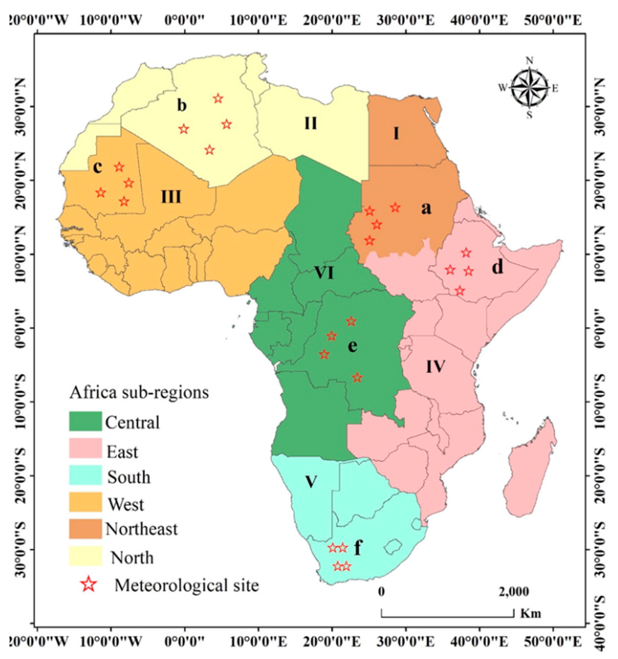
2.1. Study Area

Africa ranks among the largest continents in the world in terms of geographical vastness. Specifically, Africa has an area of approximately 30.3 million km2 and covers 6% of the Earth’s total surface area and 20% of the Earth’s land area. Africa has a variety of climatic conditions, ranging from tropical humid to arid climates. The desert/arid region covers half of the northern and savanna plains, and rainforest regions cover the central and southern areas. Of all continents, Africa is the warmest, and the Sahara Desert covers approximately 60% of the total land area in Africa [28]. With increases in climate variability and a warming trend in sub-Saharan Africa, an increase in the seasonal mean temperature has been recorded [29]. Temperature change is a major driver of vegetation dynamics and influences the distribution of crop species and vegetation [30,31].
According to the United Nations geographic classification scheme, Africa was classified into five subregions (northern, western, central or middle, eastern and southern). The southern subregion is the smallest, and this subregion (10%) is very small compared to the northern region, which covers 27% of the total area [32]. To obtain more detail about the characteristics of LST in Africa, we classified North Africa into two regions (North Africa and northeastern Africa); thus, in this study, six subregions were used for the analysis of the LST (Figure 1). Subregion I represents northeastern Africa, where a desert-type climate is predominant across the areas south of the Mediterranean. The climate characteristics of northeastern Africa are arid, and temperatures often surpass 38 °C in Egypt; in Sudan, the mean annual temperature is approximately 26.7 °C, and annual rainfall events occur between June and September, with a total precipitation of 254 mm. The variation in climate is very conducive to the growth of crops, making the northeast region one of Africa’s most important grain- and cash crop-producing areas. Subregion II represents North Africa and spans from south of Sudan to east of the Atlas Mountains. The region is dominated by a temperate monsoon climate and high temperatures in Sahara countries such as Libya. In this region, most countries (e.g., Algeria) depend on irrigation agriculture because of limited rainfall. In Algeria, agriculture contributes to 25% of the economy, and less than 14% of the total land area there is suitable for agriculture. Subregion III represents West Africa, which includes 16 countries from Mauritania to Togo, where dry and hot continental air masses and wet equatorial air masses strongly impact the climate. Monsoon rain in summer is affected by the transport of equatorial wet air across the Atlantic Ocean [33]. The Guinean Highlands have more precipitation than the lowlands at the same latitude, ranging from 1600 mm to 165 mm. However, maximum temperatures can reach above 40 °C. Deforestation is the most prominent environmental issue that dominates West Africa, where the rate of deforestation is the highest. Subregion IV represents East Africa, which is a typical equatorial region. The topography is represented by high land, and the metrological conditions are typical of rainy conditions in equatorial regions, where the Rwenzori Mountains and Ethiopian Highlands create strong winds. Surprisingly, East Africa is cool and dry across its latitudes. Notably, the coast of Somalia has experienced drought for many years. In East Africa, rainfall and temperature are influenced by El Niño events, except for the areas in the humid coastal belt, which have a moderate maximum temperature of approximately 25 °C. Subregion V represents South Africa, where the conditions are dominated by temperatures below 20 °C because the area is located between the Atlantic Ocean and the Indian Ocean. The weather during the warm season in this subregion is influenced by the El Niño–Southern Oscillation (ENSO). During an El Niño phase, the weather in South Africa is hot and dry, and La Niña phases are accompanied by cool and wet conditions. Subregion VI represents Central Africa, which has rainforest conditions (along the equator) with climate conditions ranging from warm to hot with very high humidity. Notably, the heaviest rainfall in Africa is recorded in this area, which contains 89.3% of the total swamp forest and lowland humid areas in Africa. This region has dense vegetation that is key to Africa’s climate and environment.

2.2. MODIS Data

MODIS data are used worldwide to support scientific studies of a broad range of land and ocean phenomena [34,35]. MODIS LST data produced from two satellites, Terra and Aqua that were launched in 1999 and 2002 respectively, are available twice daily. Terra passes over the equator at 10:30 and 22:30 from north to south, and Aqua passes the equator at 13:30 and at 1:30 from south to north. The satellites are maneuvered in a near-polar, sun-synchronous orbit at an altitude of 705 km, each providing global surface temperature data with high accuracy and quality [36].
In this study, monthly data (MOD11C3/MYD11C3) from the Terra and Aqua satellites that were available for the period of 2003–2017 were used, and quality control (QC) layers were used to ensure the reliability of each LST pixel. The National Aeronautics and Space Administration (NASA) provided the daytime and nighttime surface temperatures in the collection 6 data series provided in 2017 [37]. The cloud-contaminated LST pixels in collection 6 were removed from the level 2 swath product (geophysical product that remains in latitude and longitude orientation) and level 3 daily and eight-day products (geophysical product that has been temporally and or spatially manipulated). Additionally, pixels influenced by other variables (e.g., particles, aerosols, and varying sun angles) that affected the accuracy of the data at a spatial resolution of 0.05° × 0.05° (more than 5000 m at the equator) were removed.
The MODIS products were re-projected to the WGS-84 datum and geographic coordinate system using the MODIS Projection Tool (MRT) for nearest neighbor resampling, and the data format was transformed to TIFF format. For the day and night LST data layers that were selected using ArcGIS (10.2), the LST was converted from Kelvin to Celsius.

2.3. Ground Observation Data

Meteorological observation sites data in Africa is very scarce, because of that we have to use temperature data from CRU time series dataset version 4.03 from 2003 to 2017 (https://crudata.uea.ac.uk/cru/data/temperature). We calculate the difference between the MODIS land surface temperature product and the air temperature from CRU in the vicinity of the weather in clear day conditions, and use the difference as a correction for air temperature data from CRU under cloud condition, and then interpolate it into the remote sensing temperature product. These enhanced CRU datasets used as inputs in the reconstruction model to fill the gaps associated with MODIS LST data missing values and enhance the data quality. Furthermore, we extracted the LST values by using a similar previous method at the locations of meteorological stations to validate the MODIS LST data (Figure 1). The 24 meteorological stations selected for verification were located in the most critical countries based on cooling and warming trends (Figure 1), which were not used in the reconstruction procedure. Elevation data at a 1-km spatial resolution were available from the NASA Space Shuttle Radar Terrain Mission V4.1 (SRTM) for the reconstruction of cloud-contaminated data.

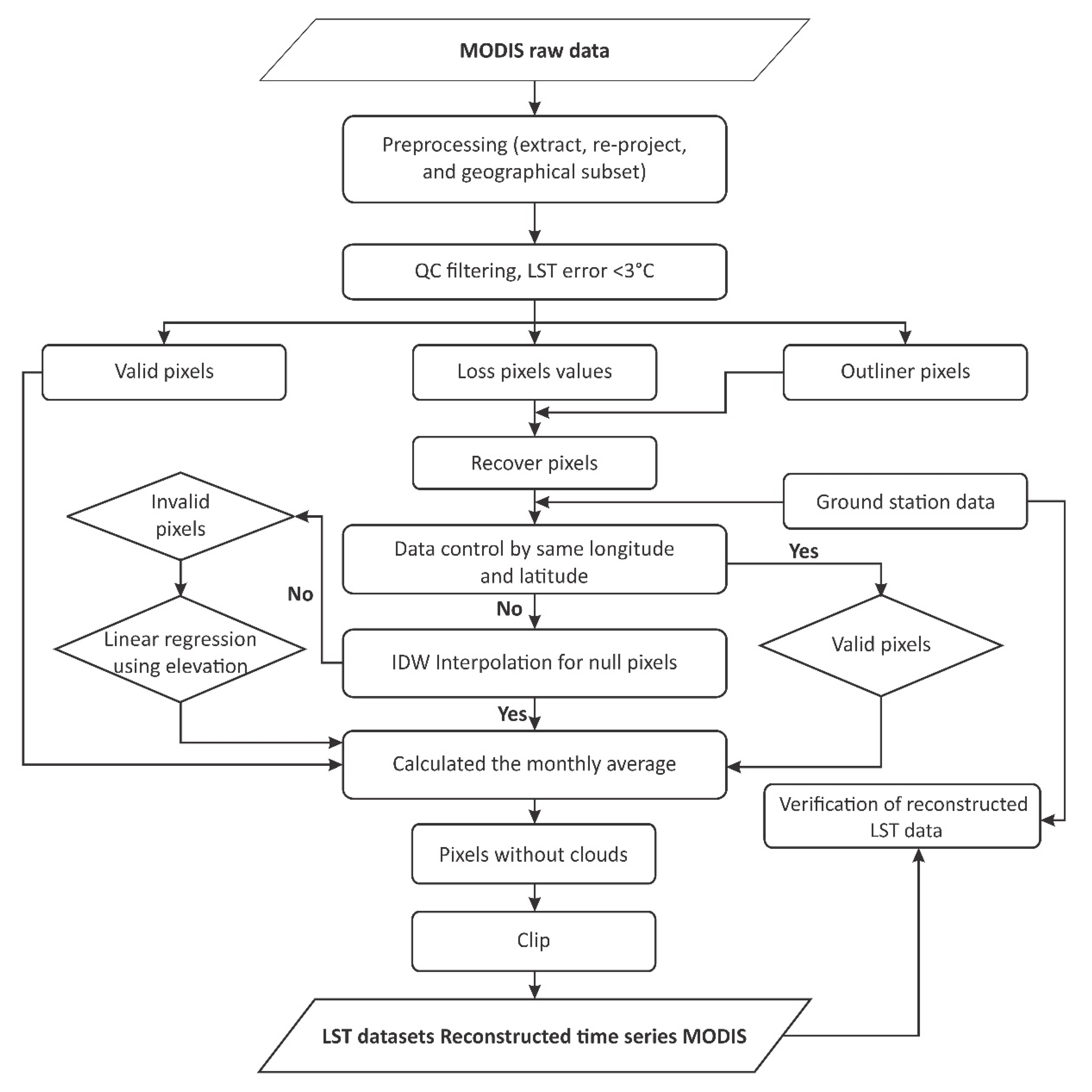
2.4. LST Data Reconstruction Method

In this study, we present a reconstruction model that is dependent on meteorological station data (Figure 2). The procedures used in this model include four main steps. First, to obtain valid data, we used the QC layer for filtering to determine the null and contaminated pixel values (i.e., the missing and poor-quality pixels) and applied the enhanced ground station data including modified ground surface temperature by using air temperature from CRU (see Section 2.3) at the same longitude and latitude to fill the null pixels. Then, the IDW method was used to interpolate contaminated pixels using valid pixels from the direct filling gaps. Finally, after interpolation, we used linear regression to fill the data in the invalid pixels.

2.5. LST Pixel Filtering

LST time series data retrieved from thermal infrared bands often contain invalid data due to contamination from various types of noise. Therefore, these values must be identified and filtered. To remedy this issue, a reliable method for removing low-quality pixels was applied using the data QC information for each MODIS LST product. All pixels with an LST error <3 °C were filtered using the appropriate MODIS LST QC level (quality indicator levels in the MODIS LST HDF files) [38,39]. To ensure high data quality, we filtered and eliminated inferior pixels using QC labels. After filtering using the QC layer, the spatial distribution pattern of invalid data was displayed after the quality of the Terra and Aqua satellite LST data were filtered, as shown in Figure 3. The data are shown in Figure 3. These LST data for February 2017 and August 2017 represent the missing night time values during autumn months, day time values during summer months and the distribution of some low-quality pixel values. As shown in Figure 3a,c, the coverage of low-quality pixels was 18.14% for Terra and 8.1% for Aqua. There are many missing values in North Africa in summer, and in winter, the rain forest zones in Central Africa, South Africa, and Ethiopia have many missing values, as these areas are affected by extensive rainfall during these seasons.

2.6. LST Data Recovery

First, a traditional method was employed using ground station data to fill the null pixels in MODIS LST data at the same location. The mean values for the valid ground-based LST data were used to fill the pixels with null LST values influenced by cloud cover, and these filled pixels were marked. Then, because of weather station data were not enough the IDW method based on neighboring pixels was applied to interpolate contaminated pixels using valid pixels from the direct areas around gaps, which is the underlying assumption of IDW. IDW is very flexible and most common spatial interpolation method than other interpolation methods, if there are ridges in a different elevation profile and climate zone, then this is the appropriate method. The value at a non-sampled point is a weighted average of the values at the nearby measured points, the weights are generally the inverse distance squared, the nearest measured points are defined as those located within a given distance or the nearest n-points [40,41]. This method assumes that the neighboring pixels have significant similarities that are proportional to the distance between each pixel and the target pixel (reverse function), and we used weighted average of three surrounding pixels. The accuracy of this method mainly depends on the number and quality of neighboring pixels.
Z 0 = i = 1 N Z i . d i n i = 1 N d i n
where Z 0 = the estimated (reconstructed) LST value of a null pixel I, Z i = the weight average of three neighboring known pixel value at target point I, i = a target pixel null value, d i = the weight average distance between the three known pixels value with unknown pixel value, n = the coefficient used to define the weight based on distance, and N = the total number of estimations.

2.7. Estimation of Invalid Pixel Values

Then, we used a linear regression formula between LST and elevation to retrieve unknown LST values that did not have enough neighboring pixels with known values. The linear regression relationships for unknown pixel values were constructed based on scanning each pixel in the image with a sliding window to obtain empty pixel values and the neighboring pixel values. We used a small window size ( 50 × 50   Km 2 ) that covered approximately 2500 km2, which is an appropriate size for identifying cloud effects and more sensitive than larger windows [42]. If the neighbors of the target pixel (null value) are valid and at least 15% of the LST pixels in the window are valid, the scanning and estimation step continues until there are no null pixel values in the image. The null pixel values were estimated using the following equation [43]:
V = L × ρ i + φ
where V is an LST value estimated via interpolation (units: °C), ρ is the elevation (units: m), L is the assessed regression coefficient of the elevation considering the LST, and φ is the predicted intercept.

2.8. Validation

The accuracy of the reconstructed LST was assessed based on a set of statistical metrics, including the correlation coefficient (R), root mean square error (RMSE), and mean absolute error (MAE). The equations of these statistical measures are as follows:
R = i = 1 n (   x i x ) ( y i y ) (   x i x ) 2 ( y i y ) 2
where R is the correlation coefficient, x i is reconstructed data, y i is ground station data from the ith year, x is the overall average of the reconstructed data and y is the average of the ground station data for the study period (15 years). In this case, R ranges from −1 to +1.
M A E = i = 1 n [ x i y i ] n
R M S E = i = 1 n ( x i y i ) 2 2
where n is the number of study period years (15 years), y i represents the reconstructed pixel values, and x i represents the station values. The RMSE is an indicator that reflects the bias in the mean and spatial variance. The MAE reflects the error magnitude, and low values indicate excellent performance [44].

2.9. Mean LST

After generating a high-precision monthly dataset, Africa’s LST was calculated from MODIS data to determine the month and year that were the warmest and coldest to help estimate seasonal changes in Africa. The mean daily temperatures at different satellite overpass times (t) (1:30, 10:30, 13:30, and 22:30) were calculated using the following equation:
L m i z = 1 n p = 1 p = n L S i z
where L m i represents the mean LST of pixel i at time z and p is a specific day of the year. The mean LST in Africa at time z was calculated using the following equation.
L m z = 1 n p = 1 p = n j = 1 j = m S ( i ) S L p i Z
where L m z is the mean LST at time z, i is the specific day of the month, p is the pixel index, and S ( i ) is the area weighting function. S L p i Z is the LST at a certain time (1:30, 10:30, 13:30, or 22:30) of each month. The monthly mean LST at time t in Africa during the study period was computed using the following equation.
L m = ( L m 1 : 30 + L m 10 : 30 + L m 13 : 30 + L m 22 : 30 ) / 4
where L m is the mean LST. The warmest and coldest months from 2003 to 2017 were May and September, respectively. In this study, the overall Africa seasons were classified based on Northern Hemisphere seasons, because more than about two-thirds of Africa located in Northern Hemisphere. The classification based on three months per season as follows: spring (end of March, April, May, and June), Summer (end of June, July, August, and September), Autumn (end of September, October, November, and December), and Winter (end of December, January, February, and March).

2.10. Trend Analysis of Change (Slope) and the Correlation Coefficient (R)

In this study, to investigate the significant upward and downward trend of annual and monthly LST time series the nonparametric Mann Kendall test [45,46] was used in Africa for the period 2003–2017. In addition, the homogeneity of LST data is examined in order to identify break points in the middle time series using the Pettit test method [47]. These two methods have been proved to be a very useful tool to quantify the significance and magnitude of change in hydroclimatic data. The methodologies of these statistical tests are broadly documented [48,49,50].
The changes in the trends of various time series (monthly, seasonally, and yearly) were considered to evaluate the variations in the spatiotemporal patterns of the MODIS LST based on Equation (9). The monthly time series were transformed into a yearly time series. The time series for each pixel had a length of n = 15, spanning from 2003 to 2017. The rate of change was applied to estimate the regional trend using linear regression with the effects of the constant bias inherent in the data considered negligible [51,52,53,54,55]. Thus, we assessed the interannual variations in LST from the slope [51,55]. Equation (10) [56] was used to compute the LST time series correlation coefficient (R) from 2003 to 2017 at different time scale annually, monthly, seasonally, and day and night.
S = n Y = 1 n ( Y × W m Y ) Y = 1 n Y Y = 1 n W m Y n Y = 1 n Y 2 ( Y = 1 n Y ) 2
R = n Y = 1 n ( Y × W Y ) Y = 1 n Y Y = 1 n W Y n Y = 1 n Y 2 ( Y = 1 n Y ) 2 × n Y = 1 n W Y 2 ( Y = 1 n W Y ) 2
where n is the range of the study period; Y is the number of years ( Y = 1, 2, 3 … n, in this paper, where n = 15); and W Y represents the LST in year Y . Notably, W Y is computed from Aqua and Terra. When the slope value approaches 0, there are no significant changes in the trend. A slope > 0 indicates an increasing trend, and a slope < 0 represents a decreasing trend [57]. The R-value extends from negative to positive correlations (−1 to +1). An R-value < 0 indicates that the LST is negatively correlated with the time series, and an R-value > 0 suggests that the LST is positively correlated with the time series. The significance of the trend was evaluated using the F-Test (CORRCOEF- function) at each pixel, and a p-value less than 0.05 was considered statistically significant.

3. Results

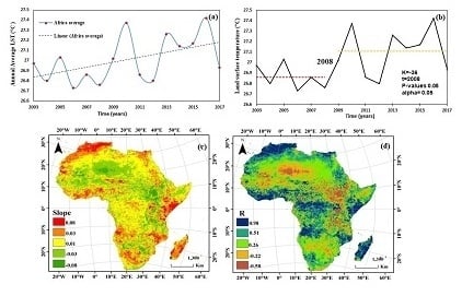
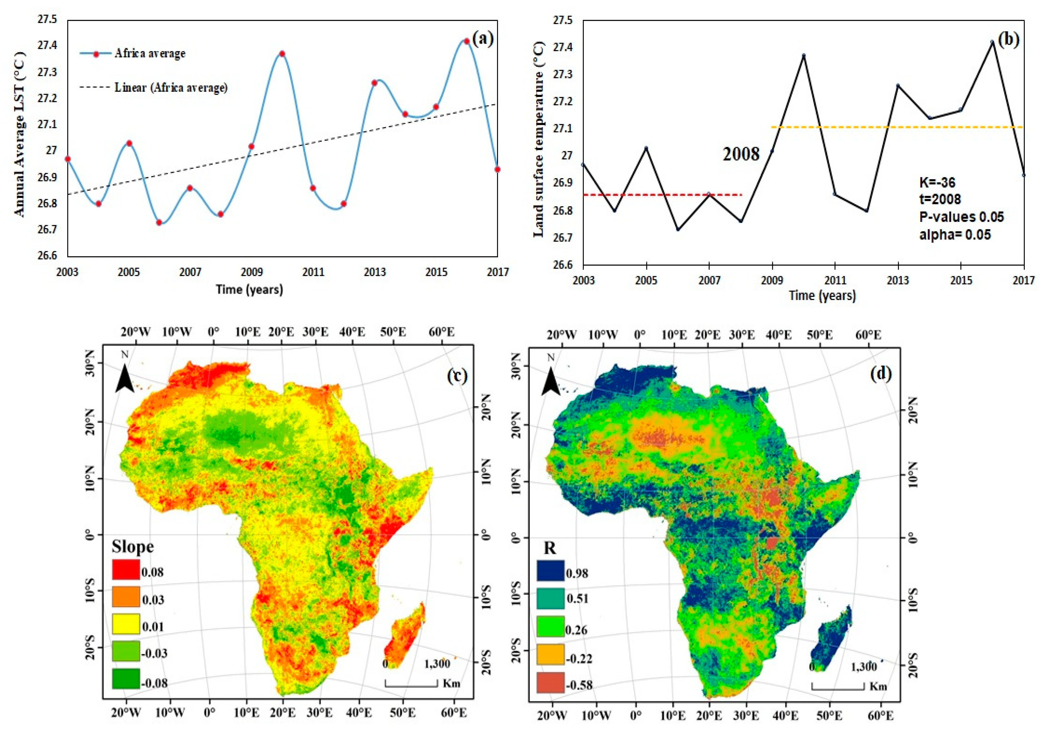
3.1. Annual Change Analysis

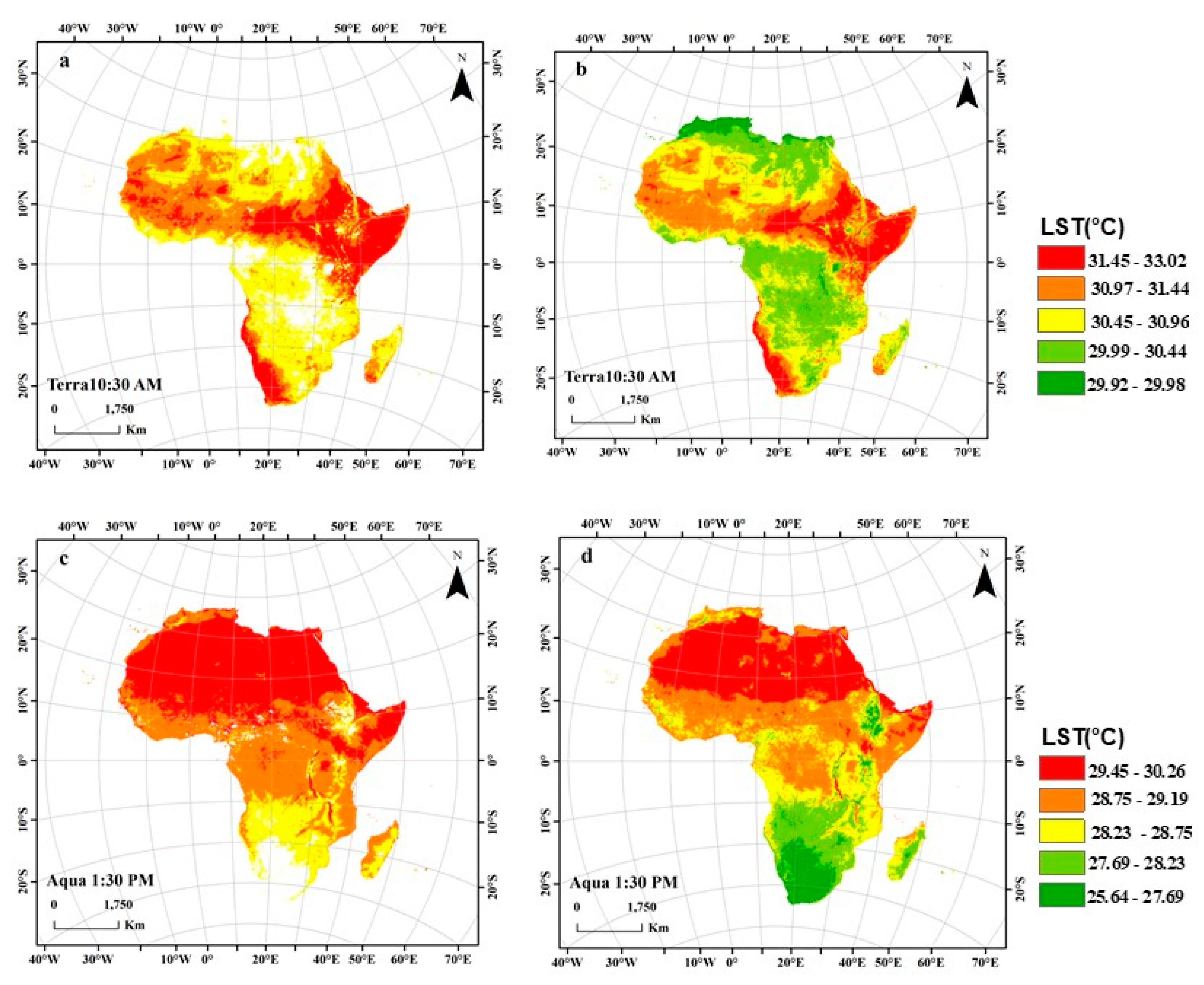
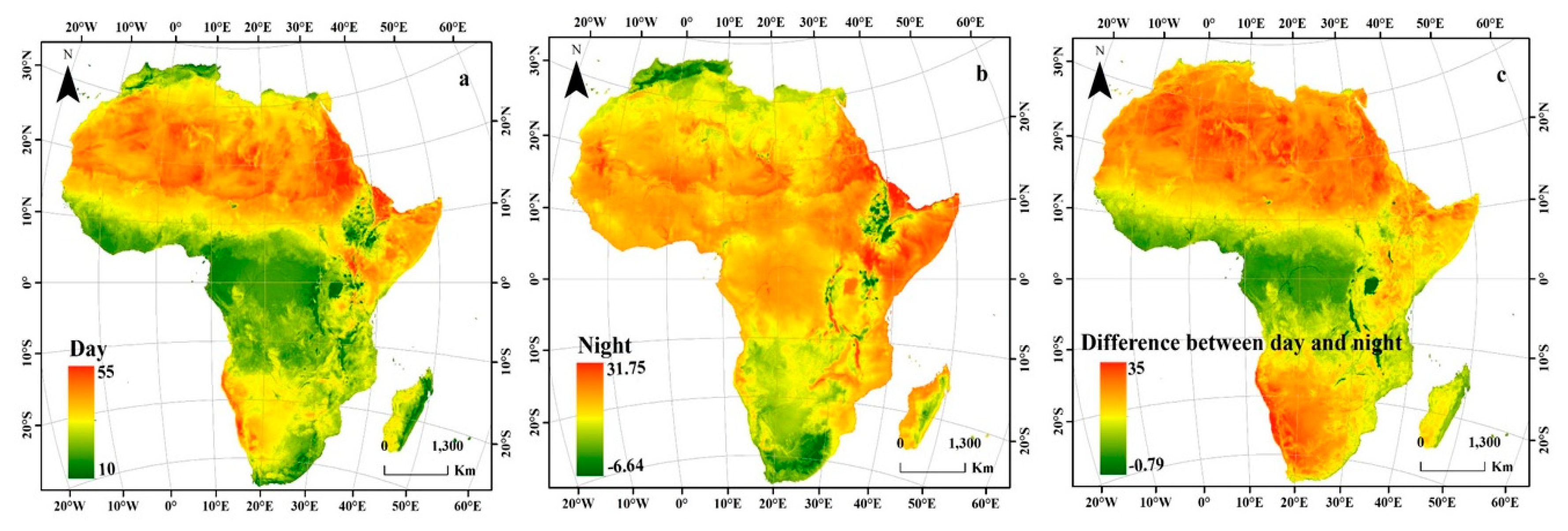
3.1.1. Average LST Change

To understand the overall LST trend we calculate the average of each year, Mann-Kendall test performed to verify a significant upward or downward trend, and used the Pettitt test to demonstrate change occurred in Africa, over the period from 2003–2017. The mean annual LST (°C) was found to vary across the continent during this period, as shown in Figure 4a. The coldest year was 2006 (26.73 °C), and the warmest year was 2016 (27.42 °C). The coldest and the warmest years differed by approximately 0.69 °C. We show the main reasons for the decrease in the LST in 2016, which could be due to the El Niño event [58]. The annual trends of mean temperature by the Mann–Kendall test are given in Table 1. In can be observed that trends for LST time series were statistically significant at α = 0.05 level of significance. LST series show upward and downward trends throughout the study period, while overall trend Z with positive value means the trend is increasing. However, Pettit’s procedure (Figure 4b) shows that the significant upward shift for mean temperature has occurred since 2008. The slowdown in global warming has been greatly affected by the El Niño/Southern Oscillation (ENSO) [59]. In recent years, one of the most important reasons for the increase in temperature and the deceleration of climate change has been the cooling of the La Niña stage during the evolution of ENSO. Additionally, other natural activities, such as volcanic eruptions and solar activities, have increased the surface temperature [60]. The regional distribution of the LST trend (Figure 4c), the correlation coefficient (Figure 4d) and the significance of the trend (Supplementary Figure S1) in each subregion were calculated on an annual basis to determine the spatiotemporal variation. The LST displayed the highest significant warming trend in many countries in northwestern regions, but negative trends occurred in some eastern and southern regions; moreover, the positive trend in the mountains was greater than that in wetland areas, such as those surrounding Lake Victoria. The increase in trends with high significance covers 56% (from >99%*** to >90%*) of highland areas, such as the Atlas Mountains and the Ethiopian Plate, as well as Burkina Faso.
In contrast, the desert zone, especially the northern region (Chad and Niger) and the southern region in Botswana, was mainly characterized by a nonsignificant decrease in LST during the study period (Supplementary Figure S1). The LST trend was nonsignificant and reflected cooling in the regions of Sahara countries such as Algeria and Sudan and regions around water resources such as Lake Victoria (Figure 4c). A warming trend was observed in the Atlas Mountains near the Mediterranean Sea, Madagascar and the tip of southern Africa near the Indian Ocean, with a significantly higher trend than other areas. The frequency distribution of the percentage of the area in Africa that experienced a warming trend (slope > 0.1) accounted for 76.56% of the total area in highland regions, such as the Atlas Mountains, Ethiopia Plateau, and Central Africa (savanna zones and forests land). In contrast, 23.44% of countries displayed a cooling trend (slope < −0.1), and the area with a significant cooling pattern (slope > −0.07) covered 6.17% of the total area and was mainly concentrated in mid-to-northern Africa.
In 2016, due to a decline in precipitation during winter and early spring in northern Africa (north of the Atlas Mountains and along the Mediterranean coast of Algeria and Tunisia), the LST experienced significant warming. However, a nonsignificant decrease (slope > −0.08), which contributed to the African cooling trend, was observed in the northeastern region of Africa (subregion I). We observed widespread and relatively strong cooling and nonsignificant cooling in most of the region near the Red Sea Mountains (slope > −0.06, R > 0.8, p < 0.05). Attention should be paid to the countries in the northeast because they produce important commercial grain products (sorghum, wheat, millet, etc.) and cash crops (cotton, gum arabic, and sesame). Furthermore, 24% of the land in Sudan is cultivated, and it is the most important producing country, representing 17% of the grain production in Africa, with sorghum accounting for 45% of the total cultivated land. Intensified low temperatures could cause insufficient heat accumulation during the crop growing period, which would reduce the crop yield. Moreover, if this rapid cooling continues in the northeast region, it will pose a great threat to agricultural manufacturing and regional economic growth. The relevant agricultural sectors should be aware of the possible effects, and suitable preventive and regulatory measures should be taken.
In the North Africa region (subregion II), the mean slope value was 0.03, and the spatial variations in LST exhibited interesting characteristics: the trend was opposite on either side of the Atlas Mountains and in North Africa (slope > −0.07, R > −0.8, p < 0.05, Figure 4c,d), except in the highlands of the Atlas Mountains where the slope was high and change was significant at >99%** (slope > 0.085, R > 0.8, p < 0.05). Furthermore, Mount Toubkal to the east of the Atlas Mountains has a high elevation and exhibited an upward trend (Figure 4).
In West Africa (subregion III), the climate was similar in the northwest African part of the Sahara and the savanna zones. A slight but significant LST trend was observed in southern West Africa (slope < −0.16, R < −0.88 P > 0.05, Figure 4c,d), which suffered from a decline in vegetation in the last half of the 20th century, especially in Senegal [61]. Deforestation along the southern coast of West Africa can cause a significant reduction in rainfall and affect monsoon circulation. This process can also increase the frequency and intensity of drought, resulting in the degradation of fragile local vegetation, the shrinking of oasis areas and an increase in the vulnerability of the ecological environment. Finally, due to the sparse vegetation south of the West region, such as in Nigeria, there is a need for increased ecological engineering, such as the Three-North Shelterbelt Program. Furthermore, an increase in vegetation cover is conducive to increasing the soil water content, which can improve local land desertification and ever-expanding soil erosion. Additionally, in terms of vegetation, the regulation of greenhouse gases and evapotranspiration at the local scale could generate positive feedback on the stability of surface temperatures.
In the eastern Africa region (subregion IV), we observed significant warming in coastal areas such as Somalia, and Madagascar is of great interest (slope > 0.06 R > 0.8, p < 0.05, Figure 4b–d; high significance of >99%***, Supplementary Figure S1). The significant warming trend in East Africa in recent years may be related to increasing global sea surface temperatures [62]. East Africa is considered the main region for African water resources. For instance, Dutra et al. [63] indicated that a strong La Niña event was the main cause of the 2010–2011 drought in Horn Africa. Tierney et al. [64] also suggested that the recent drought experienced in the Horn of Africa was partly due to the prevailing La Niña conditions in the tropical Pacific, and the authors noted that rainfall variability in eastern Africa was driven by the Indian Ocean through the alteration of the local Walker circulation. Moreover, many problems, such as forest fires, deforestation, urban expansion, mining activities, and land degradation, have occurred in these areas.
The trend in Central Africa (subregion VI, Figure 4c,d) exhibited almost no change (slope > 0.07, R > 0.8, p = 0.05) and low significance > 90*, which may be due to deforestation and increased greenhouse gases. Forests are capable of decreasing the LST [65,66,67]. The forests in Central Africa are the second-largest rainforest block on the planet and the key to the global environment. In South Africa (subregion V) (Figure 4c,d), the trend in the southwest significantly increased (slope > 0.08, R > 0.89, p < 0.05, Figure 4c,d), and a nonsignificant decreasing trend was observed in Botswana. Therefore, surface warming has mainly occurred in the Sahara in Africa, as urbanization has influenced the regional temperature [68].

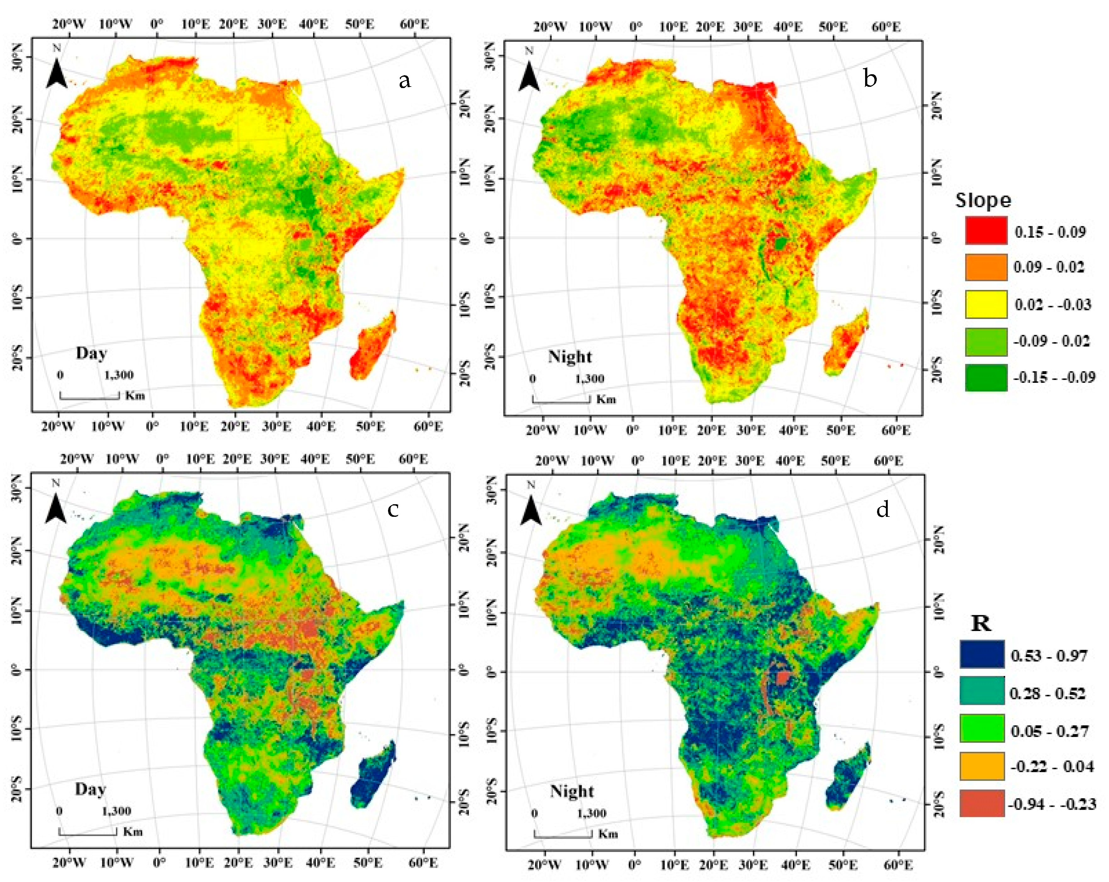
3.1.2. Daytime and Night Time Change Analysis

To further investigate the LST variations in detail over Africa, the daytime and nighttime LST trends were analyzed, as shown in Figure 5, along with the significance of outputs (Figure S2). The results in Figure S2 show that the night time trend is more significant (>99% ***) than the daytime trend, with highly significant increasing trends of 8.14% and 3.23%, respectively. However, during the day, the nonsignificant cooling trends were concentrated in East Africa near the Red Sea, Horn of Africa, Nile, African lakes and rainforest zone in Central Africa (Figure 5, Supplementary Figure S2). The frequency distribution of significant warming trends during the day with slopes > 0.076 covered 22.5% of the entire region, especially in Sierra Leone and Liberia, with a significance of >99%***. At night, the warming trends were highly significant (slope < −0.07, R < 0.8, significant trend > 99%**) in areas close to the Atlas Mountains, near the outlet of the Nile River basin, in the Namibian Desert and in Madagascar.
However, at night, the heat released by the surface is absorbed while most heat is radiated back to space by the atmosphere. In the highlands during the warm period, the trend decreased during the day and increased at night, which suggests that the warmest temperature occurred at night [69]. This variation in LST from day to night is indicative of human activities and solar characteristics during the daytime [70].

3.1.3. Analysis of the Diurnal Temperature Difference

During the day, the distribution of LST varied with surface irradiance as a function of the solar zenith angle [71]. Figure 6 shows the spatial distribution of the average daytime and nighttime LSTs and the difference in LST between day and night. We found a significant spatial variation gradient in LST. Notably, the highest LST occurred during the day (Figure 6a) in North, West, and East Africa in desert areas (32 °C to more than 40 °C) but not in the low-latitude areas south of the tropics; however, this trend differed at night. The Sahara in North Africa has enormous potential for generating solar energy, as Africa is considered the warmest continent in the world. The relatively high albedo of the Sahara Desert makes it warmer than other areas due to high solar radiation during the day. In areas with high levels of sunlight, such as the Sahara, frequent changes in temperature often occur due to warming and cooling when the local albedo changes [72]. In the Atlas Mountains, the nocturnal LST at high elevations decreased from south to north, and the spatial variation approximately reflected the five subregions. This result also suggests that the temperature changes are significantly related to the proximity to the equator. Figure 6c shows that the largest diurnal difference in LST is mainly concentrated in the highland areas above 25 °C. The high values of the daily differences between day and night LST are mainly concentrated in the desert areas of North Africa and South Africa to the west above 35 °C, as shown in Figure 6. The lowest daily LST difference occurred at the low latitudes of Central Africa (~29 °C) over lakes such as Victoria and on the southeast coast (Madagascar). The high heat capacity of water reduces the diurnal temperature range in relation to that of the surrounding landscape, with a counterintuitive relationship with albedo. Low heat absorption during the day due to high albedo should reduce energy availability at night, as demonstrated in the Sahara area [73].

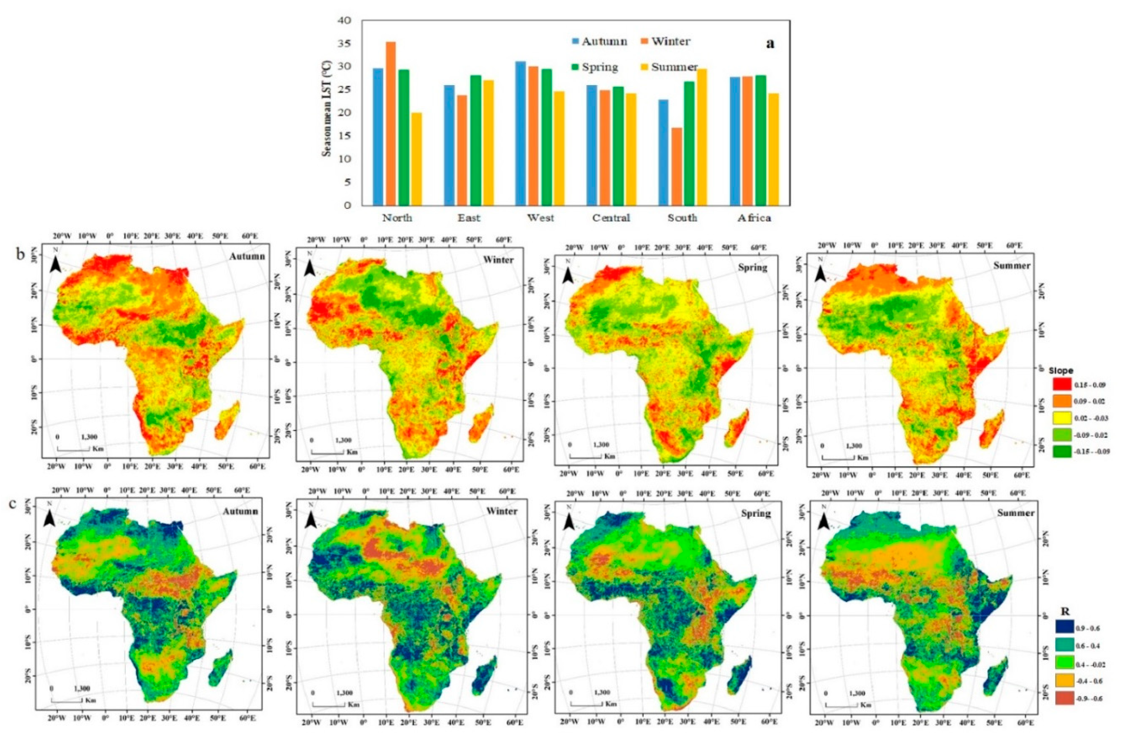
3.2. Seasonal Change Analysis

Based on the classification of the areas in the Northern Hemisphere, seasonal variations have a significant effect on LST across Africa. The mean seasonal LST of the African continent changed significantly (see Figure 7a, Supplementary Figure S3). Overall, our results indicate the average LST was lowest in summer with high significance from >99%*** to >95%** over 32.5% of the continent, especially in southern Africa (29.54 °C); the main reason for this trend is the variation in the seasonal temperature. The maximum temperature of 29.47 °C was observed in the winter season in western Africa.
In the winter season, the frequency distribution of the warming trend (slope > 0.05) covered 67.67% of the areas observed to be warm, which was significantly higher than that in the other seasons (45.6% of the total area displayed a significant trend). Therefore, winter represents an important time for the changes in the annual average, as the LST increases during winter. The most notable warming trend occurred in the western region (subregion III), especially in Mauritania (slope > 0.09, R > 0.58), and the trend was significant at >99%***. In particular, these large-scale rapid warming trends in winter should be noted. Among these trends, the LST increased in the northwest region, specifically in the central and western areas (most of the surface slopes > 0.07, R > 0.51, and significance > 95**) and in coastal areas near the Atlantic. In Madagascar (slope > 0.08, R > 0.72, and high significance levels ranging from >99%*** to >95%**), the LST increased considerably due to the increase in the temperature of the Indian Ocean. Across West Africa, the temperature increases occurred in combination with the increase in global temperatures over the past five decades [74]. However, the effects of global warming on precipitation in West Africa are difficult to assess in a climate that has been highly volatile over multiple time scales.
In the spring, a nonsignificant trend covered most of Africa (49.15%) (Figure S3), and a warming trend dominated in subregions I, III, and VI. Additionally, in northern Africa (subregion II), limited cooling was noted, with the exception of the warming of the Atlas Mountains. In the central region (subregion VI), the Atlas Mountains and Madagascar showed dramatic warming trends, where the slope was greater than 0.05 (see Figure 7b), which explains why the temperature changes in the Indian Ocean are still unclear [75]. In addition, in eastern Africa (IV), spring was noted to be the most warmed season, with a nonsignificant trend, and a negative and highly significant trend was detected in other seasons. There was rapid warming in the western Horn of Africa (slope > 0.06, R = 0.68, and mostly nonsignificant). Temperature increases have an effect on forest growth and productivity and can alter the LST, increase the drought risk, aggravate seasonal degradation, and reduce water availability. Moreover, the risk of forest fire is increased by drought, which is fueled by shrubs and dry trees.
As indicated in Figure 7 and Supplementary Figure S3, in the summer season across the country, a significant warming trend was noted. In Northeast Africa (subregion I), the trend decreased and was nonsignificant, including in south Egypt and south Sudan (slope < −0.09 and R < 0.8), and increased near the coast of the Red Sea (slope < 0.09 and R < 0.8, and with a significant trend > 99%***). In these areas, the months from December to February correspond to the end of the growing season. In North Africa (subregion II), the connection between climate change and rising temperatures may reduce the coverage of arable land, shorten vegetation periods and reduce crop yields. In the autumn season, the trend in West Africa (subregion III) increased slightly (slope > 0.07, R > 0.59, and highly significant trend from >99%*** and >95%**) and decreased in Mauritania with a nonsignificant trend. Significant trends were observed in southern countries in the Sahel Belt, such as Nigeria. Nigeria, however, is in a region with a high risk of drought, and as the temperature across Nigeria increased from 1971–2012 [76], precipitation decreased by 20% from 1901–2000 [77]. The lack of reports of devastating droughts over the past few decades underscores the need to understand how recent climate changes have affected droughts in Africa.

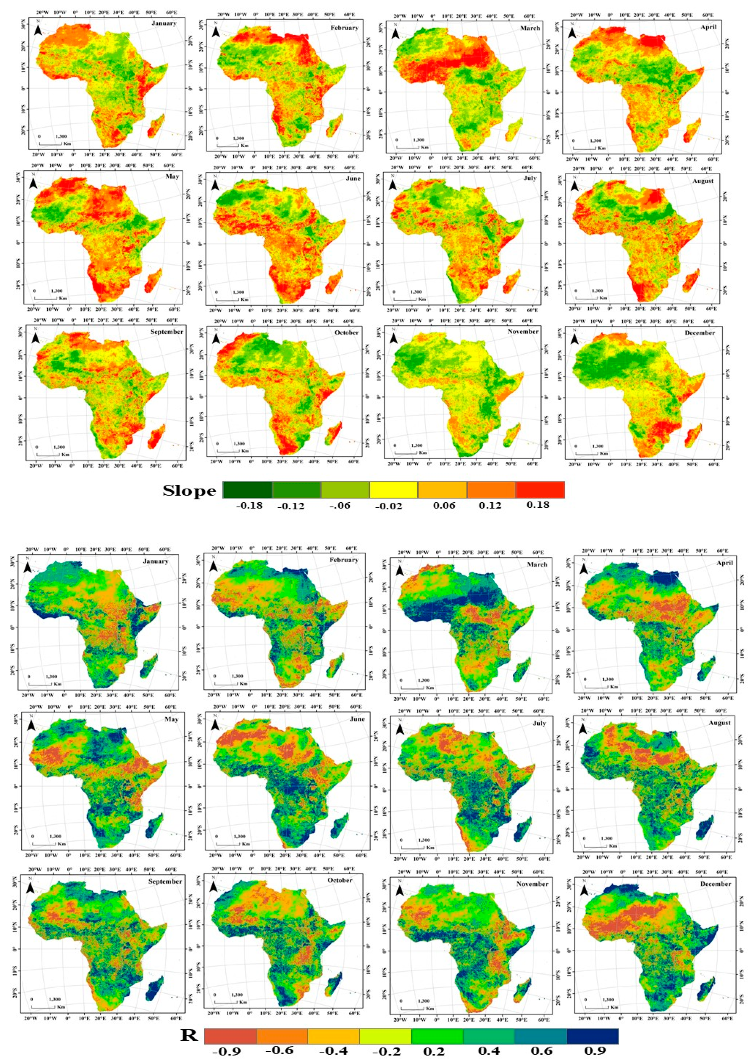
3.3. Monthly Average Change Analysis

An analysis of the overall monthly trend and average monthly changes in LST from 2003 to 2017 is presented in Table 1 and Figure 8, respectively, and the significance of the trend is shown in Figure S4. The Mann Kendall test used to investigate a significant upward or downward monthly trend throughout the study period was varied, within different levels of significance. It can be seen that all the 12 months showed an increasing trend for monthly mean temperature, with a total of two months having statistical significance α = 0.05 (June* and July*), and 0.01 of September**.
The warming trend was significant, especially in the months of April, May, August, and September. The maximum warming trend and significance level were observed in May (slope > 0.07, significance was >99%***), and 83% and 64% of the areas exhibited warming and significant trends, respectively. Relatively significant warming (slope > 0.08, significant trend > 99%***) occurred in the highlands of North Africa, the coastal areas and the northeast. In September, the temperatures were relatively high, with a warming trend in 69% of the study area and a significant trend in 72% of the area. The mountains in Africa are concentrated in the northwest, and the Atlas Mountains experienced significant warming. In the warmer months with significant trends; however, there was no significant cooling trend. The broadest cooling trend was widespread close to the water resource and coastal areas of Africa, with a nonsignificant trend. In the northeast, the cooling trend began in November, December, and January in South and Central Africa. The monthly changes in LST from 2003 to 2017, which were recorded in May and September, showed a strong upward and significant trend. In West Africa and the highlands, the trend was obviously increasing and highly significant at >99%***. The results are consistent with those of Sylla et al., and such extreme increases are mainly due to intense variations in the local water cycle [78]. In addition, the lack of rainfall and increasing drought have significantly influenced the temperature changes in West Africa [79]. The warmest temperatures have had a major negative impact on the major crops in Africa, such as corn and sorghum [80].

3.4. Validation

Different methods have been used to reconstruct LST and exhibited good performance in filling missing pixels, as has been validated by various studies [42,56,81]. In this study, the dataset was verified using independent in situ measurements that were not used in the reconstruction model (Figure 1 in Section 2.1). Therefore, all ground-based LST data were used to check the accuracy of the rebuilt data in regions with drastic changes (see Figure 9 for more information). Six countries were selected based on warming and cooling trends as critical zones. These countries include the four most important warming countries (Figure 9a–d) and the two most important cooling countries (Figure 9e,f). We used the correlation coefficient (R), the RMSE, and the MAE to evaluate the accuracy of the new LST data model. The correlation coefficient (R) of all stations varied from 0.84 to 0.96 with an average of 0.90. The RMSE ranged from 0.81 °C to 1.55 °C with an average of 1.10 °C. By comparison, a large RMSE between the ground-based LST and rebuilt LST occurred in some locations in South Africa (Figure 9, Region f), where the temperature is impacted by the complex terrain and forest areas. The MAE varied from 0.56 °C to 1.11 °C with an average of 0.75 °C. This result indicates that the reconstructed MODIS LST dataset, due to the high consistency with in situ information, is robust and accurate. The main areas used for the review are cases where the local heating/cooling frequency of the LST changes more than the overall rate and the theoretical error rate is larger than that in other regions. In addition, the examples show that the reconstruction model proposed here is efficient in the most likely error domains. As the temperature data are further adjusted to better reflect the general temperature trend, the trends in other regions should become more accurate. Therefore, we believe that this approach can guarantee the accuracy of LST data.
To obtain a better understanding of the credibility of the information, the accuracy of the seasonal predictions was assessed. In the six main areas (Figure 1), the MAE values of the ground-based LST data and the respective LST data were used to assess the seasonal variations, as shown in Table 2. The summer season has the largest average MAE of 1.14 °C, followed by spring with a value of 1.08 °C. In addition, the MAE values at some of the sites were substantially higher in the summer than in the other seasons. These sites were mainly located in West Africa (Mauritania), which may be due to the complicated and variable terrain there, wide range of climatic variations, and the influence of the Ethiopian Plateau in the western region. These values were comparatively low in four other areas, including Sudan, Algeria, Congo, and South Africa. The winter MAE ranged from 0.08 °C to 3.52 °C with an average of 1.03 °C. Moreover, the distribution of MAE varied greatly between the eastern and western regions at the seasonal scale. For all stations in the eastern typical zones (i.e., key zone (a) in northeast region (I) and key zone (b) in the North Africa region (I)), the maximum MAE values occurred in summer, and the highest values at most sites in the western region occurred during the summer (i.e., the remaining four zones). Additionally, a comparison of the results suggests that the mean MAE of the ground-based observation data and the LST data in the eastern region was significantly higher than that recorded in the western region (mean 1.42 °C in eastern region I and 0.98 °C in western region III). In the eastern region, the spatial heterogeneity of temperature due to the complex terrain may be the cause of large errors.
The verification results demonstrate that the dataset is in reasonable agreement with the station measurements, indicating that the cloud cover interference was well resolved. The accuracy and spatial and temporal continuity of this dataset are significantly improved compared to that for the monthly MODIS original data. We believe that this dataset can be used in research on the regional ecological environment and for monitoring agrometeorological disasters. In a few practical applications, such as urban heat island monitoring, our current data may not be able to provide sufficient detail due to the coarse resolution, and this issue should be improved in future work.

4. Discussion

The issue of climate change in Africa is well worth studying. Temperature changes are key factors influencing and controlling climate change in certain identifiable ways. Africa is certainly a developing continent, hence, many countries do not have enough weather stations. Consequently, a lack of weather stations leads to poor data coverage and the inability to record temperature changes across the continent. Researchers reported that remote sensing data may be a reliable alternative to compensate for this shortage [82]. In this study, the spatiotemporal changes in LST in Africa for 15 years were investigated using long-term sequences of MODIS data. This study we reconstructed LST dataset for Africa from 2003 to 2017 based on a ground-measured temperature dataset and ground weather station data from the Terra and Aqua MODIS satellites. To analyze the spatiotemporal variations in LST, we reconstructed a model based on an LST time series and ground station data and recreated the LST record. Then, the MODIS LST reconstructed data was analyzed to provide a detailed description of the significant patterns of LST. The dataset was used to examine the regional characteristics and variations in LST at the monthly, seasonal and interannual scales. The LST displayed a slight upward trend (76.56% for warming and approximately 23.44% for cooling, with 56% of the trends being significant). The strongest significant warming trend was observed in the south, followed by the trends in the Atlas Mountains and western East Africa (Madagascar). The impacts of human activities, such as urbanization, industrial and agricultural development, deforestation and wildfires, had a tremendous effect on warming. However, this trend was more pronounced in fast-growing urban areas such as South Africa and in areas with abundant water resources. Additionally, a nonsignificant cooling trend was observed in other parts of Africa; the north became noticeably colder (slope < −0.07, R > −0.85), and there was a slight cooling trend in West Africa (slope < 0). Moreover, the temperature during the nighttime changed more significantly than that during the day, which may be closely related to the changes in solar radiation and the release of large amounts of greenhouse gases by human activities.
Different surface types at different times react to different temperature changes. Our results suggest that the LST was high during the day, as solar radiation is a major source of heat, leading to a massive increase in LST (Figure 5). In contrast, the source of heat at night comes from the heat trapped during the day. Therefore, the trend during the day decreased and the trend at night increased in the highlands, with a strong correlation between nighttime and daytime patterns [69]. This information helps to better understand local warming and climate regimes, which are important in shaping agricultural production.
Earth rotation is the determining factor for seasonal change. The rotation of the Earth influences the monsoon changes, ocean currents, and other factors. Our results showed that there were significant differences in the LST trends in different seasons. The warming trend in winter was the most significant compared to that in the other three seasons, especially in West Africa (Mauritania, see Figure 8), the Atlas Mountains, the Ethiopian Plateau region, and the Sahel due to low rainfall (July, August, September, and October). Studies by Leroux et al. [83] showed the same results, as the winter season was warmer than the other seasons. In the summer and spring seasons, the green areas (savannas and forests) and coastal areas are affected by temperature decreases due to evapotranspiration. The results are in agreement with those of Kebiao et al. [84], who reported that an increase in green space lowered the surface temperature of the land. Similar results showed that the rate at which the temperature changed in the Sahara differed from that in other areas due to the lack of vegetation and water scarcity, which confirms the possible relationship between temperature and green space and the direct influence on climate change [80].
Overall, the temperature in the Sahara region is moderate and the temperature change rate between day and night was recorded to be between low and medium trends. The most significant month seems to be September, however, except for the Sahara region, the trend of surface temperature changes across Africa is increasing. This study reveals that the Sahara region has an impact on surface to show increased or decreased trend of LST which can explain and define the relationship between LST and vegetation.
In controlled environmental studies, the rate of phonology increases with increasing temperature, and it does not affect vegetation biomass compared to normal temperatures. The warmest temperature has a large negative impact on the main crop yield in Africa such as maize and sorghum [50]. The reduction in vegetation cover results an increased production of atmospheric carbon dioxide and there is an interaction among vegetation, evaporation, and carbon dioxide, since green land work regulates the temperature and carbon dioxide in the atmosphere. In the warmest time (months, seasons, and years) vegetation degradation led to elevated temperatures and carbon dioxide, consequently, the rate of increase in carbon dioxide causes global warming. Based on the results obtained in this study, we may opine and consider the change in surface temperature to be critical, which is important for predicting the consequences that the globe might face in the wake of climate change. Therefore, remote sensing technology provides data, basically covering the African continent.
Critical LST changes are important for predicting the consequences that could be faced globally in the context of climate change events in Africa. In African countries, there are regular droughts due to insufficient rainfall and high temperatures. When we summarized the LST trend from 2003 to 2017, we observed significant changes in some regions of Africa, including the hottest and coldest years on record, differences between day and night, and seasonal changes. In addition to climate change, decreasing vegetation coverage in Africa, which is mainly caused by drought and population growth, is increasing the LST. Without radical decentralization measures, however, it will be difficult to prevent or reverse the urbanization process in forest areas as population and economic growth spur the demand for natural resources [85,86]. The implementation of sustainable development and growth management strategies can help to limit the reduction in forest areas.

5. Conclusions

Analyzing the spatiotemporal changes in LST is important for understanding the distribution of warming trends. The spatiotemporal changes in LST were investigated using a long-term sequence of MODIS data in Africa (2003–2017) in this study. This pixel reconstruction process has hardly been applied in Africa on such a scale to analyze the spatiotemporal changes in LSTs. An approach for reconstructing LST was used to get long-term sequence LST data over Africa based on IDW interpolator and liner regression model. The results of the spatiotemporal analysis of the overall annual average LST showed that the LST fluctuated and that the warming trend in Africa was remarkably heterogeneous. LST time series with high spatial and temporal resolutions are crucial for various applications. As a crucial environmental factor and an important indicator of climate change, the LST in Africa is increasing gradually. The results suggest that 2016 was a highly significant warming year and 2006 was a nonsignificant cold year. A highly significant warming trend was generally observed at the diurnal, seasonal, and monthly time scales. However, the most significant warming LST trend occurred near the equator in the south and central regions. These significant trends imply increased LSTs despite the fact that LSTs have varied interannual and spatially. At the diurnal scale, the LST was typically increased during the day in mid-North Africa compared with the trends in the annual and seasonal periods. Spatially, a highly significant warming trend was identified in the winter season, especially in Mauritania.
Moreover, LST changes are key factors that influence and control climate change in different ways. Thus, government agencies and climate-relevant organizations must pay particular attention to the changes in the LST to characterize climate change. Urbanization and population growth are also part of the cause of LST change, in addition to climate change. Without radical decentralization measures, however, it will be difficult to prevent or reverse the urbanization of forest areas, as population and economic growth increase the need for natural resources.

Supplementary Materials

The following are available online at https://0-www-mdpi-com.brum.beds.ac.uk/2072-4292/12/3/488/s1, Figure S1: Significance of the spatial distribution of annual LST trends in Africa from 2003 to 2017, Figure S2: Spatial dynamics of the significant diurnal variations in diurnal LST change from 2003 to 2017, Figure S3: Significance of the spatial distribution of seasonal LST trends from 2003 to 2017, Figure S4: Significance of the spatial distribution of monthly LST trends in Africa from 2003 to 2017.

Author Contributions

N.N. and K.M. conceived the research; N.N. wrote the manuscript; N.N. and K.M. edited the manuscript; and N.N., K.M. and Z.Y. contributed to the data analyses. All authors have read and agreed to the published version of the manuscript.

Funding

This research was funded by the National Key R&D Program Key Project (Global Meteorological Satellite Remote Sensing Dynamic Monitoring, Analysis Technology and Quantitative Application Method and Platform Research (2018YFC1506502) & Multi-source meteorological data fusion technology research and product development (2018YFC1506602)), the National Natural Science Foundation of China (41571427) and the Open Fund of State Key Laboratory of Remote Sensing Science (Grant no. OFSLRSS201910).

Acknowledgments

The authors would like to thank the National Aeronautics and Space Administration (NASA) for their support with the LST products and elevation data.

Conflicts of Interest

The authors declare no conflicts of interest.

References

  1. Tan, J.; Noureldeen, N.; Mao, K.; Shi, J.; Li, Z. Deep learning convolutional neural network for the retrieval of land surface temperature from AMSR2. Sensors 2019, 19, 2987. [Google Scholar] [CrossRef] [PubMed] [Green Version]
  2. Li, Z.; Tang, B.; Wu, H.; Ren, H.; Yan, G.; Wan, Z.; Trigo, I.F.; Sobrino, J.A. Satellite-derived land surface temperature: Current status and perspectives. Remote Sens. Environ. 2013, 131, 14–37. [Google Scholar] [CrossRef] [Green Version]
  3. Arnon, K.; Nurit, A.; Rachel, T.P.; Martha, A.; Marc, I.F.; Garik, G.; Gutman; Natalya, P.; Alexander, G. Use of NDVI and land surface temperature for drought assessment: Merits and limitations. J. Clim. 2009, 23, 618–633. [Google Scholar] [CrossRef]
  4. Beurs, K.M.D.; Henebry, G.M. Land surface phenology, climatic variation, and institutional change: Analyzing agricultural land cover change in Kazakhstan. Remote Sens. Environ. 2004, 89, 497–509. [Google Scholar] [CrossRef]
  5. Kumar, K.S.; Bhaskar, P.U.; Padmakumari, K. Estimation of land surface temperature to study urband heat island effect using landsat ETM + image. Int. J. Eng. Sci. Technol. 2012, 4, 771–778. [Google Scholar]
  6. Dash, P.; Göttsche, F.M.; Olesen, H.; Fischer, F.S. Land surface temperature and emissivity estimation from passive sensor data: Theory and practice-current trends. Int. J. Remote Sens. 2010, 37–41. [Google Scholar] [CrossRef]
  7. Laura, P. Climate change impacts on agriculture across Africa. Oxford Res. Encycl. Environ. Sci. 2017, 1–35. [Google Scholar] [CrossRef]
  8. Serdeczny, O.; Adams, S.; Coumou, D.; Hare, W.; Perrette, M. Climate change impacts in Sub-Saharan Africa: From physical changes to their social repercussions. Reg. Environ. Chang. 2016, 17. [Google Scholar] [CrossRef]
  9. Itai, K.; Francesco, N.; Coull, B.A.; Schwartz, J. Predicting spatiotemporal mean air temperature using MODIS satellite surface temperature measurements across the Northeastern USA. Remote Sens. Environ. 2014, 150. [Google Scholar] [CrossRef]
  10. Guo, Z.; Wang, S.D.; Cheng, M.M.; Shu, Y. Assess the effect of different degrees of urbanization on land surface temperature using remote sensing images. Procedia Environ. Sci. 2012, 8, 962–969. [Google Scholar] [CrossRef] [Green Version]
  11. Yuan, X.; Wang, W.; Cui, J.; Meng, F.; Kurban, A. Vegetation changes and land surface feedbacks drive shifts in local temperatures over Central. Sci. Rep. 2017, 3–10. [Google Scholar] [CrossRef] [PubMed] [Green Version]
  12. Meyer, H.; Katurji, M.; Appelhans, T.; Müller, M.U.; Nauss, T.; Roudier, P.; Zawar-Reza, P. Mapping daily air temperature for Antarctica based on MODIS LST. Remote Sens. 2016, 8, 732. [Google Scholar] [CrossRef] [Green Version]
  13. Ozelkan, E.; Bagis, S.; Ozelkan, E.C. Spatial interpolation of climatic variables using land surface temperature and modified inverse. Int. J. Remote 2015, 36. [Google Scholar] [CrossRef]
  14. Justice, C.O.; Vermote, E.; Townshend, J.R.G.; Defries, R.; Roy, D.P.; Hall, D.K.; Salomonson, V.V.; Privette, J.L.; Riggs, G.; Strahler, A.; et al. The Moderate Resolution Imaging Spectroradiometer (MODIS): Land remote sensing for global change research. IEEE Trans. Geosci. Remote Sens. 1998, 36, 1228–1249. [Google Scholar] [CrossRef] [Green Version]
  15. Hengl, T.; Heuvelink, G.B.M. Spatio-temporal prediction of daily temperatures using time-series of MODIS LST images. Theor. Appl. Climatol. 2012, 265–277. [Google Scholar] [CrossRef] [Green Version]
  16. Wan, Z. New refinements and validation of the collection-6 MODIS land-surface temperature/emissivity product. Remote Sens. Environ. 2014, 140, 36–45. [Google Scholar] [CrossRef]
  17. Mao, K.B.; Yuan, Z.J.; Zuo, Z.Y.; Xu, T.R.; Shen, X.Y.; Gao, C.Y. Changes in global cloud cover based on remote sensing data from 2003 to 2012. Chin. Geogr. Sci. 2019, 29, 306–315. [Google Scholar] [CrossRef] [Green Version]
  18. Metz, M.; Andreo, V.; Neteler, M. A new fully gap-free time series of land surface temperature from MODIS LST Data. Remote Sens. 2017, 9, 1333. [Google Scholar] [CrossRef] [Green Version]
  19. Neteler, M. Estimating daily land surface temperatures in mountainous environments by reconstructed MODIS LST data. Remote Sens. 2010, 2, 333–351. [Google Scholar] [CrossRef] [Green Version]
  20. Fan, X.; Liu, H.; Liu, G.; Li, S. Reconstruction of MODIS land-surface temperature in a flat terrain and fragmented landscape. Int. J. Remote Sens. 2014, 37–41. [Google Scholar] [CrossRef]
  21. He, J.; Zhao, W.; Li, A.; Wen, F.; Yu, D. The impact of the terrain effect on land surface temperature variation based on Landsat-8 observations in mountainous areas. Int. J. Remote Sens. 2018, 40, 1–20. [Google Scholar] [CrossRef]
  22. Lyon, S.W.; Rasmus, S.; Stendahl, J. Using landscape characteristics to define an adjusted distance metric for improving kriging interpolations. Int. J. Geogr. Inf. Sci. 2010, 37–41. [Google Scholar] [CrossRef] [Green Version]
  23. Yu, W.; Nan, Z.; Wang, Z.; Chen, H.; Wu, T.; Zhao, L. An effective interpolation method for MODIS land surface temperature on the Qinghai–Tibet plateau. IEEE J. Sel. Top. Appl. Earth Obs. Remote Sens. 2015, 8, 4539–4550. [Google Scholar] [CrossRef]
  24. Shiode, N.; Shiode, S. Street-level spatial interpolation using network-based IDW and ordinary kriging. Trans. Gis. 2011, 15, 457–477. [Google Scholar] [CrossRef]
  25. Pede, T.; Mountrakis, G. An empirical comparison of interpolation methods for MODIS 8-day land surface temperature composites across the conterminous Unites States. ISPRS J. Photogramm. Remote Sens. 2018, 142, 137–150. [Google Scholar] [CrossRef]
  26. Wang, Z.; Peng, B.; Zhou, W. Reconstructing spatial–temporal continuous MODIS land surface temperature using the DINEOF method. J. Appl. Remote Sens. 2017. [Google Scholar] [CrossRef]
  27. Evgenieva, T.; Iliev, I.; Kolev, N.; Sobolewski, P.; Pieterczuk, A. Optical characteristics of aerosol determined by cimel, prede, and microtops ii sun photometers over belsk, poland. In Proceedings of the 15th International School on Quantum Electronics: Laser Physics and Applications, Bourgas, Bulgaria, 15–19 September 2008; Volume 7027, pp. 1–8. [Google Scholar] [CrossRef]
  28. Khalid, I.E.F.; Randall, S.; Christopher, C.B.; Philip, E.D.P.; Manola, B.; Thomas, C.P.; Gianpaolo, M.; Vinicio, P.; Pierre, B.; José, L.S.; et al. World meteorological organization assessment of the purported world record 58°C temperature extreme at El Azizia, Libya (13 September 1922). Am. Meteorol. Soc. 1997. [Google Scholar] [CrossRef]
  29. Measho, S.; Chen, B.; Trisurat, Y.; Pellikka, P.; Guo, L. Spatio-temporal analysis of vegetation dynamics as a response to climate variability and drought patterns in the Semiarid Region, Eritrea. Remote Sens. 2019, 11, 724. [Google Scholar] [CrossRef] [Green Version]
  30. Martin, T. Climate change impacts: Vegetation. Encycl. Life Sci. 2009. [Google Scholar] [CrossRef]
  31. Na-u-dom, T.; Mo, X.; Garcίa, M. Assessing the climatic effects on vegetation dynamics in the Mekong river basin. Environments 2017, 4, 17. [Google Scholar] [CrossRef] [Green Version]
  32. Sedami, A.; Yevide, I.; Bingfang, W.U.; Xiubo, Y.U.; Xiaosong, L.I.; Yu, L.I.U.; Jian, L.I.U. Building African ecosystem research network for sustaining local ecosystem goods and services. Chin. Geogr. Sci. 2015, 25, 414–425. [Google Scholar] [CrossRef] [Green Version]
  33. Abdrabo, M.; Ama, E.; Lennard, C.; Adelekan, I.O. Chapter 22 Africa. In Climate Change 2014: Impacts, Adaptation, and Vulnerability. Part B: Regional Aspects. Contribution of Working Group II to the Fifth Assessment Report; Cambridge Univ. Press: Cambridge, UK; New York, NY, USA, 2014; pp. 1199–1265. [Google Scholar]
  34. Kaufman, Y.J.; Herring, D.D.; Ranson, K.J.; Collatz, G.J. Earth observing system AM1 mission to Earth. IEEE Trans. Geosci. Remote Sens. 1998, 36, 1045–1055. [Google Scholar] [CrossRef]
  35. Ban, H.; Kwon, Y.; Shin, H.; Ryu, H.; Hong, S. Flood monitoring using satellite-based RGB composite imagery and refractive index retrie val in visible and near-infrared bands. Remote Sens. 2017, 9, 313. [Google Scholar] [CrossRef] [Green Version]
  36. Vancutsem, C.; Ceccato, P.; Dinku, T.; Connor, S.J. Evaluation of MODIS land surface temperature data to estimate air temperature in different ecosystems over Africa. Remote Sens. Environ. 2010, 114, 449–465. [Google Scholar] [CrossRef]
  37. Kilpatrick, K.A.; Podestá, G.; Walsh, S.; Williams, E.; Halliwell, V.; Szczodrak, M.; Brown, O.B.; Minnett, P.J.; Evans, R. A decade of sea surface temperature from MODIS. Remote Sens. Environ. 2015, 165, 27–41. [Google Scholar] [CrossRef]
  38. Benali, A.; Carvalho, A.C.; Nunes, J.P.; Carvalhais, N.; Santos, A. Remote sensing of environment estimating air surface temperature in Portugal using MODIS LST data. Remote Sens. Environ. 2012, 124, 108–121. [Google Scholar] [CrossRef]
  39. Metz, M.; Rocchini, D.; Neteler, M. Surface temperatures at the continental scale: Tracking changes with remote sensing at unprecedented detail. Remote Sens. 2014, 6, 3822–3840. [Google Scholar] [CrossRef] [Green Version]
  40. Lecture Notes for MEA592 Geospatial Analysis and Modeling. Available online: https://ncsu-geoforall-lab.github.io/geospatial-modeling-course/resources/interpolation_notes.pdf (accessed on 12 August 2019).
  41. Attorre, F.; Alfo, M.; De Sanctis, M.; Bruno, F. Comparison of interpolation methods for mapping climatic and bioclimatic variables at regional scale. Int. J. Climatol. 2007, 1843, 1825–1843. [Google Scholar] [CrossRef] [Green Version]
  42. Ke, L.; Song, C.; Ding, X. Reconstructing complete MODIS LST based on temperature gradients in Northeastern Qinghai-Tibet plateau. Int. Geosci. Remote Sens. Symp. 2012, 3505–3508. [Google Scholar] [CrossRef]
  43. Yan, Y.B.; Mao, K.B.; Shi, J.C.; Piao, S.L.; Shen, X.Y.; Dozier, J.; Liu, Y.; Ren, H.L.; Bao, Q. Driving factors of LST anomalous changes in North America in 2002-2018. Sci. Rep. 2019. under review. [Google Scholar]
  44. Res, C.; Willmott, C.J.; Matsuura, K. Advantages of the mean absolute error (MAE) over the root mean square error (RMSE) in assessing average model performance. Clim. Res. 2005, 30, 79–82. [Google Scholar]
  45. Mann, H.B. Nonparametric tests against trend. Econometrica 1945, 13, 245–259. [Google Scholar] [CrossRef]
  46. Kendall, M.G. Rank Correlation Methods, 4th ed.; Charles Griffin: London, UK, 1975; p. 212. [Google Scholar]
  47. Pettitt, A.N. A Non-parametric to the Approach Problem. Appl. Stat. 1979, 28, 126–135. [Google Scholar] [CrossRef]
  48. Salarijazi, M.; Adib, A.; Daneshkhah, A. Trend and change-point detection for the annual stream-flow series of the Karun River at the Ahvaz hydrometric station. Afr. J. Agric. Res. 2012, 7, 4540–4552. [Google Scholar] [CrossRef] [Green Version]
  49. Partal, T.; Kahya, E. Trend analysis in Turkish precipitation data. Hydrol. Process. 2011, 2026, 2011–2026. [Google Scholar] [CrossRef]
  50. Omer, A.; Wang, W.G.; Basheer, A.K.; Yong, B. Integrated assessment of the impacts of climate variability and anthropogenic activities on river runoff: A case study in the Hutuo River Basin, China. Hydrol. Res. 2017, 416–430. [Google Scholar] [CrossRef] [Green Version]
  51. Taylor, P.; Stow, D.; Daeschner, S.; Hope, A.; Douglas, D.; Petersen, A.; Myneni, R.; Oechel, W. Variability of the seasonally integrated normalized difference vegetation index across the north slope of Alaska in the 1990s. Int. J. Remote Sens. 2003, 24, 37–41. [Google Scholar] [CrossRef]
  52. Stow, D.; Daeschner, S.; Hope, A.; Douglas, D.; Myneni, R.; Zhou, L. Spatial-temporal trend of seasonally-integrated normalized difference vegetation index as an indicator of changes in Arctic Tundra vegetation in the early 1990s. Int. Geosci. Remote Sens. Symp. 2001, 1, 7031–7033. [Google Scholar] [CrossRef]
  53. Li, Q.; Ma, M.; Wu, X.; Yang, H. Snow cover and vegetation - induced decrease in global albedo from 2002 to 2016. JGR Atmos. 2016, 124. [Google Scholar] [CrossRef] [Green Version]
  54. Tan, C.; Ma, M.; Kuang, H. Spatial-temporal characteristics and climatic responses of water level fluctuations of global major lakes from 2002 to 2010. Remote Sens. 2017, 9, 150. [Google Scholar] [CrossRef] [Green Version]
  55. Tan, C.; Guo, B.; Kuang, H.; Yang, H. Lake area changes and their influence on factors in arid and semi-arid regions along the Silk road. Remote Sens. 2018, 10, 595. [Google Scholar] [CrossRef] [Green Version]
  56. Zhao, B.; Mao, K.; Cai, Y.; Shi, J.; Li, Z.; Qin, Z.; Meng, X. A combined Terra and Aqua MODIS land surface temperature and meteorological station data product for China from 2003–2017. Earth Syst. Sci. 2019. under review. [Google Scholar] [CrossRef] [Green Version]
  57. Chen, Z.; Yin, Q.; Li, L.; Xu, H. Ecosystem Health Assessment by Using Remote Sensing Derived Data: A case study of terrestrial region along the coast in Zhejiang province. In Proceedings of the 2010 IEEE International Geoscience and Remote Sensing Symposium, Honolulu, HI, USA, 25–30 July 2010. [Google Scholar]
  58. Ampou, E.E.; Johan, O.; Menkes, C.E.; Niño, F.; Birol, F.; Ouillon, S. Coral mortality induced by the 2015–2016 El-Niño in Indonesia: The effect of rapid sea level fall. Biogeosciences 2017, 14, 817–826. [Google Scholar] [CrossRef] [Green Version]
  59. Garfinkel, C.I.; Butler, A.H. Reviews of geophysics the teleconnection of El Niño southern oscillation to the Stratosphere. Rev. Geophys. 2018, 57, 5–47. [Google Scholar] [CrossRef] [Green Version]
  60. Anet, J.G.; Muthers, S.; Rozanov, E.V.; Raible, C.C.; Stenke, A.; Shapiro, A.I.; Brönnimann, S. Impact of solar versus volcanic activity variations on tropospheric temperatures and precipitation during the Dalton Minimum. Clim. Past 2014, 10, 921–938. [Google Scholar] [CrossRef] [Green Version]
  61. Tappan, G.G.; Sall, M.; Wood, E.C.; Cushing, M. Ecoregions and land cover trends in Senegal. J. Arid Environ. 2004, 59, 427–462. [Google Scholar] [CrossRef]
  62. Williams, A.P.; Funk, C. A westward extension of the warm pool leads to a westward extension of the Walker circulation, drying eastern Africa. Clim. Dyn. 2011, 37, 2417–2435. [Google Scholar] [CrossRef] [Green Version]
  63. Dutra, E.; Magnusson, L.; Wetterhall, F.; Cloke, H.L.; Balsamo, G.; Pappenberger, F. The 2010–2011 drought in the Horn of Africa in ECMWF reanalysis and seasonal forecast products. Int. J. Climatol. 2013, 1729, 1720–1729. [Google Scholar] [CrossRef] [Green Version]
  64. Dyn, C.; Hoell, A.; Funk, C. Indo-Pacific sea surface temperature influences on failed consecutive rainy seasons over eastern Africa. Int. J. Clim. Dyn. 2013, 43. [Google Scholar] [CrossRef]
  65. Ming, X.; Brian, L. Temperature and its variability in oak forests in the southeastern Missouri Ozarks. Clim. Res. 1997, 8, 209–223. [Google Scholar]
  66. Rustad, L.; Campbell, J.; Dukes, J.S.; Huntington, T.; Lambert, K.F.; Mohan, J.; Rodenhouse, N. Changing climate, changing forests: The impacts of climate change on forests of the Northeastern United States and Eastern Canada. US For. Serv. 2011. [Google Scholar] [CrossRef] [Green Version]
  67. Fang, Y.; Zou, X.; Lie, Z.; Xue, L. Variation in organ biomass with changing climate and forest characteristics across Chinese forests. Forests 2018, 9, 521. [Google Scholar] [CrossRef] [Green Version]
  68. Jiang, J.; Tian, G. Analysis of the impact of land use / land cover change on land surface temperature with remote sensing. Procedia Environ. Sci. 2010, 2, 571–575. [Google Scholar] [CrossRef] [Green Version]
  69. Phan, T.N. Land surface temperature variation due to changes in elevation in Northwest Vietnam. Climate 2018, 6, 28. [Google Scholar] [CrossRef] [Green Version]
  70. Matuszko, D.; Stanisław, W. Relationship between sunshine duration and air temperature. Int. J. Climatol. 2015, 3653, 3640–3653. [Google Scholar] [CrossRef]
  71. Jin, Z.; Charlock, T.P.; Rutledge, K.; Stamnes, K.; Wang, Y. Analytical solution of radiative transfer in the coupled atmosphere—Ocean system with a rough surface. Opt. Soc. Am. 2006, 45, 7443–7455. [Google Scholar] [CrossRef]
  72. Tian, L.; Zhang, Y.; Zhu, J. Decreased surface albedo driven by denser vegetation on the Tibetan Plateau. Environ. Res. Lett. 2014, 9. [Google Scholar] [CrossRef]
  73. Liu, W. Seasonal and diurnal characteristics of land surface temperature and major explanatory factors in Harris County, Texas. Sustainability 2017, 9, 2324. [Google Scholar] [CrossRef] [Green Version]
  74. Nelson, M.I.; Njouom, R.; Viboud, C.; Niang, M.N.D.; Kadjo, H.; Ampofo, W.; Adebayo, A.; Diop, O.M. Multiyear persistence of 2 pandemic A / H1N1 In fluenza Virus Lineages in West Africa. J. Infect. Dis. 2014, 210, 121–125. [Google Scholar] [CrossRef] [Green Version]
  75. Mao, K.B.; Ma, Y.; Tan, X.L.; Shen, X.Y.; Liu, G.; Li, Z.L.; Chen, J.M.; Xia, L. Global surface temperature change analysis based on MODIS data in recent twelve years. Adv. Sp. Res. 2017. [Google Scholar] [CrossRef] [Green Version]
  76. Abatan, A.A.; Abiodun, B.J.; Lawal, K.A. Trends in extreme temperature over Nigeria from percentile-based threshold indices. Int. J. Climatol. 2016, 2540, 2527–2540. [Google Scholar] [CrossRef]
  77. Oguntunde, P.G.; Abiodun, B.J.; Lischeid, G. Rainfall trends in Nigeria, 1901–2000. J. Hydrol. 2011, 411, 207–218. [Google Scholar] [CrossRef]
  78. Sylla, M.B.; Gaye, A.T.; Jenkins, G.S. On the fine-scale topography regulating changes in atmospheric hydrological cycle and extreme rainfall over west Africa in a regional climate model projections. Int. J. Geophys. 2012, 2012. [Google Scholar] [CrossRef]
  79. Dyn, C.; Ibrahim, B.; Karambiri, H.; Barbe, L. Changes in rainfall regime over Burkina Faso under the climate change conditions simulated by 5 regional climate models. Clim. Dyn. 2013. [Google Scholar] [CrossRef] [Green Version]
  80. Hat, J.L.; Prueger, J.H. Temperature extremes: Effect on plant growth and development. Weather Clim. Extrem. 2015, 10, 4–10. [Google Scholar] [CrossRef] [Green Version]
  81. Kang, J. Reconstruction of MODIS land surface temperature products based on multi-temporal information. Remote Sens. 2018, 10, 1112. [Google Scholar] [CrossRef] [Green Version]
  82. Xu, T.R.; He, X.L.; Bateni, S.M.; Auligne, T.; Liu, S.M.; Xu, Z.W.; Zhou, J.; Mao, K.B. Mapping regional turbulent heat fluxes via variational assimilation of land surface temperature data from polar orbiting satellites. Remote Sens. Environ. 2019, 221, 444–461. [Google Scholar] [CrossRef]
  83. Leroux, L.; Bégué, A.; Lo, D.; Jolivot, A.; Kayitakire, F. Driving forces of recent vegetation changes in the Sahel: Lessons learned from regional and local level analyses. Remote Sens. Environ. 2017, 191, 38–54. [Google Scholar] [CrossRef] [Green Version]
  84. Mao, K.B.; Chen, J.M.; Li, Z.L.; Ma, Y.; Song, Y.; Tan, X.L.; Yang, K.X. Global water vapor content decreases from 2003 to 2012: An analysis based on MODIS data. Chin. Geogr. Sci. 2017, 27, 1–7. [Google Scholar] [CrossRef] [Green Version]
  85. Town, D.T.; Gondar, S.; Halefom, A.; Teshome, A.; Sisay, E.; Ahmad, I. Dynamics of land use and land cover change using remote sensing and GIS: A Case Study of. J. Geogr. Inf. Syst. 2018, 165–174. [Google Scholar] [CrossRef] [Green Version]
  86. Xu, T.R.; Guo, Z.X.; Liu, S.M.; He, X.L.; Meng, Y.Y.; Xu, Z.W.; Xia, Y.L.; Xiao, J.F.; Zhang, Y.; Ma, Y.F.; et al. Evaluating different machine learning methods for upscaling evapotranspiration from flux towers to the regional scale. J. Geophys. Res. Atmos. 2018, 123, 8674–8690. [Google Scholar] [CrossRef]
Figure 1. The study area is divided into six subregions (I, II, III, IV, V, VI), and the red stars represent the meteorological sites used for validation in six critical countries (a: Sudan, b: Algeria, c: Mauritania d: Ethiopia, e: Congo, and f: South Africa).
Remotesensing 12 00488 g001
Figure 2. Flowchart showing a summary of the method used to fill the gaps in the MODIS LST data.
Remotesensing 12 00488 g002
Figure 3. Spatial distribution of reconstructed missing values for February 2017 and August 2017 from the Terra and Aqua satellites: (a,c) original LST data; (b,d) data after interpolation (areas of invalid data are shown in white).
Remotesensing 12 00488 g003
Figure 4. Spatial distributions of annual LST in Africa: (a) mean LST, (b) Pettitt test, (c) slope, (d) correlation coefficient from 2003 to 2017.
Remotesensing 12 00488 g004
Figure 5. Spatial patterns of interannual LST changes (slope) (a) during the day and (b) at night, and correlation coefficients for (c) day and (d) night.
Remotesensing 12 00488 g005
Figure 6. Spatiotemporal patterns in the average LSTs over Africa at (a) daytime, (b) nighttime, (c) and the difference between day and night LSTs.
Remotesensing 12 00488 g006
Figure 7. Seasonal LST (°C): (a) mean, (b) slope, and (c) R from 2003 to 2017.
Remotesensing 12 00488 g007
Figure 8. The monthly variations (slope) and correlation coefficients (R) of LST from 2003 to 2017.
Remotesensing 12 00488 g008
Figure 9. Comparison of the monthly data from ground stations in different countries and the monthly MODIS LST data ((a) Sudan, (b) Algeria, (c) Mauritania, (d) Ethiopia, (e) Congo, and (f) South Africa).
Remotesensing 12 00488 g009
Table 1. Mann–Kendall statistics for mean land surface temperature in Africa during 2003–2017.
Time SeriesTest ZSignificateTime SeriesTest ZSignificate
January0.49 July2.329*
February0.395 August1.536
March1.09 September2.82**
April0.098 October0.74
May1.54 November0.59
June2.083*December0.099
Annual1.68*
** Significant at α = 0.01, * Significant at α = 0.05.
Table 2. The MAEs of the ground stations in six typical zones (Unit °C).
Region CategoryRegionKey ZoneIDSpringSummerAutumnWinter
INortheast Regiona626400.612.234.60.77
Northeast Regiona626501.23.50.670.54
Northeast Regiona626600.854.010.930.24
Northeast Regiona627210.560.060.761.23
IINorth Africa Regionb606110.512.020.660.9
North Africa Regionb606200.190.410.160.29
North Africa Regionb606402.810.340.330.11
North Africa Regionb606800.090.90.081.3
IIIWest Africa Regionc614370.713.210.40.26
West Africa Regionc614990.445.010.092.43
West t Africa Regionc616124.330.720.451.02
West Africa Regionc616300.294.230.40.61
IVEast Africa Regiond638200.170.80.323.02
East Africa Regiond638320.152.80.20.33
East Africa Regiond638620.260.230.060.57
East Africa Regiond638940.491.20.550.43
VSouth Africa Regione684243.260.031.070.94
South Africa Regione684380.360.670.821.3
South Africa Regione685122.010.080.290.92
South Africa Regione685380.230.430.263.52
VICentral Africa Regionf646010.730.864.60.77
Central Africa Regionf647090.611.020.770.08
Central Africa Regionf647500.170.491.130.21
Central Africa Regionf648600.360.40.892.93
Average 0.891.480.851.03

