Multi-Scale Evaluation of Drone-Based Multispectral Surface Reflectance and Vegetation Indices in Operational Conditions

 , , , , and
Abstract
:
1. Introduction
- What is the performance of MCA sensors with regards to measuring surface reflectance?
- (a)
- What is the accuracy of MCA derived hemispherical-conical reflectance factors? (hemispherical-conical reflectance factors (HCRF), following the terminology by [24])
- (b)
- How is HCRF accuracy influenced by the type of calibration procedure followed?
- (c)
- How consistent are HCRF products spatially and over varying vegetation cover?
- What is the performance of MCA sensors with regards to deriving vegetation indices?
- (a)
- How consistent are VI products spatially and over varying vegetation cover?
- (b)
- Are the MCA derived VIs comparable to VIs derived from similar bands of coarser spatial resolution data captured close in time (HyPlant, Sentinel 2)?
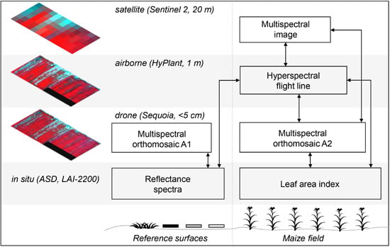
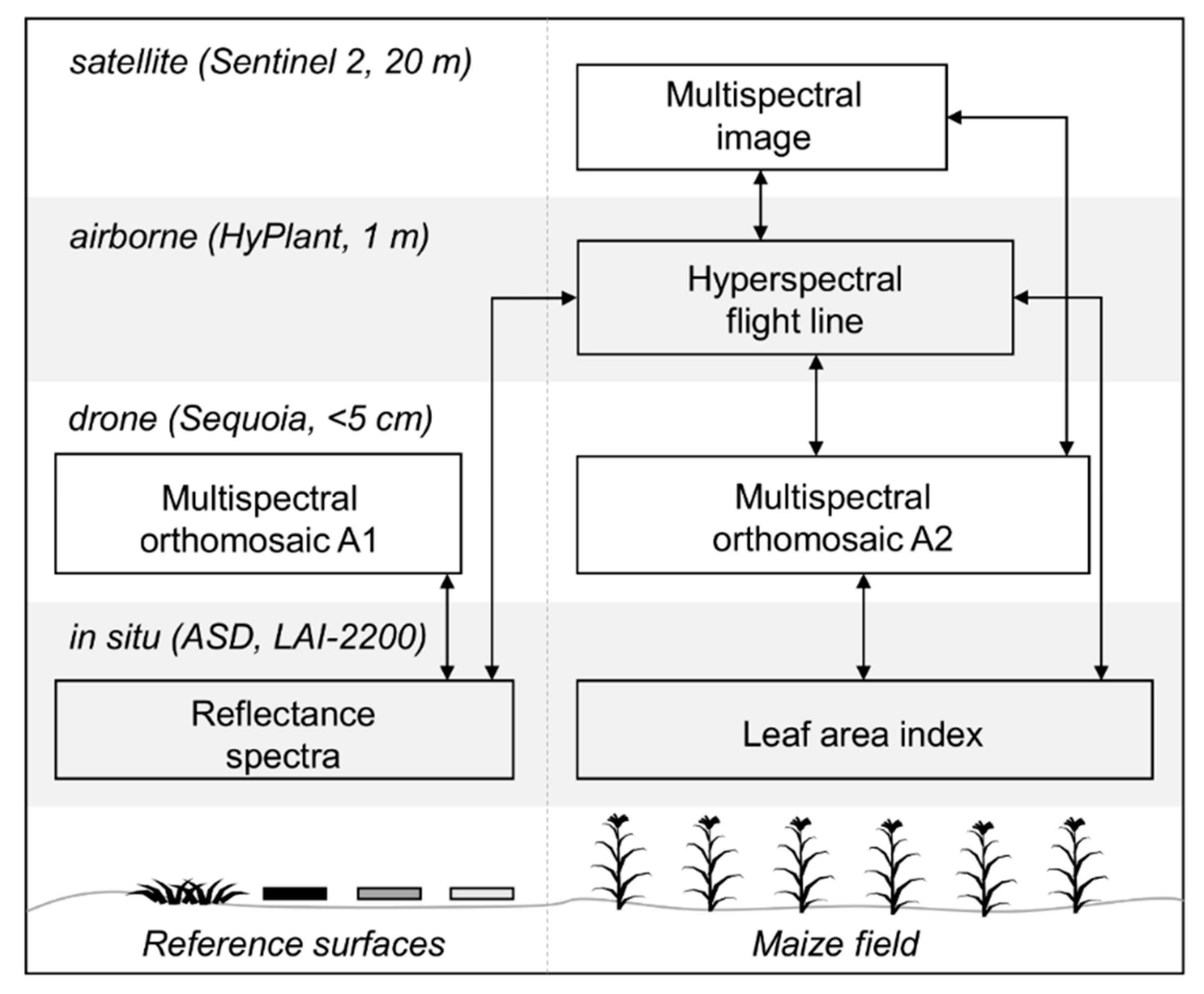
2. Materials and Methods
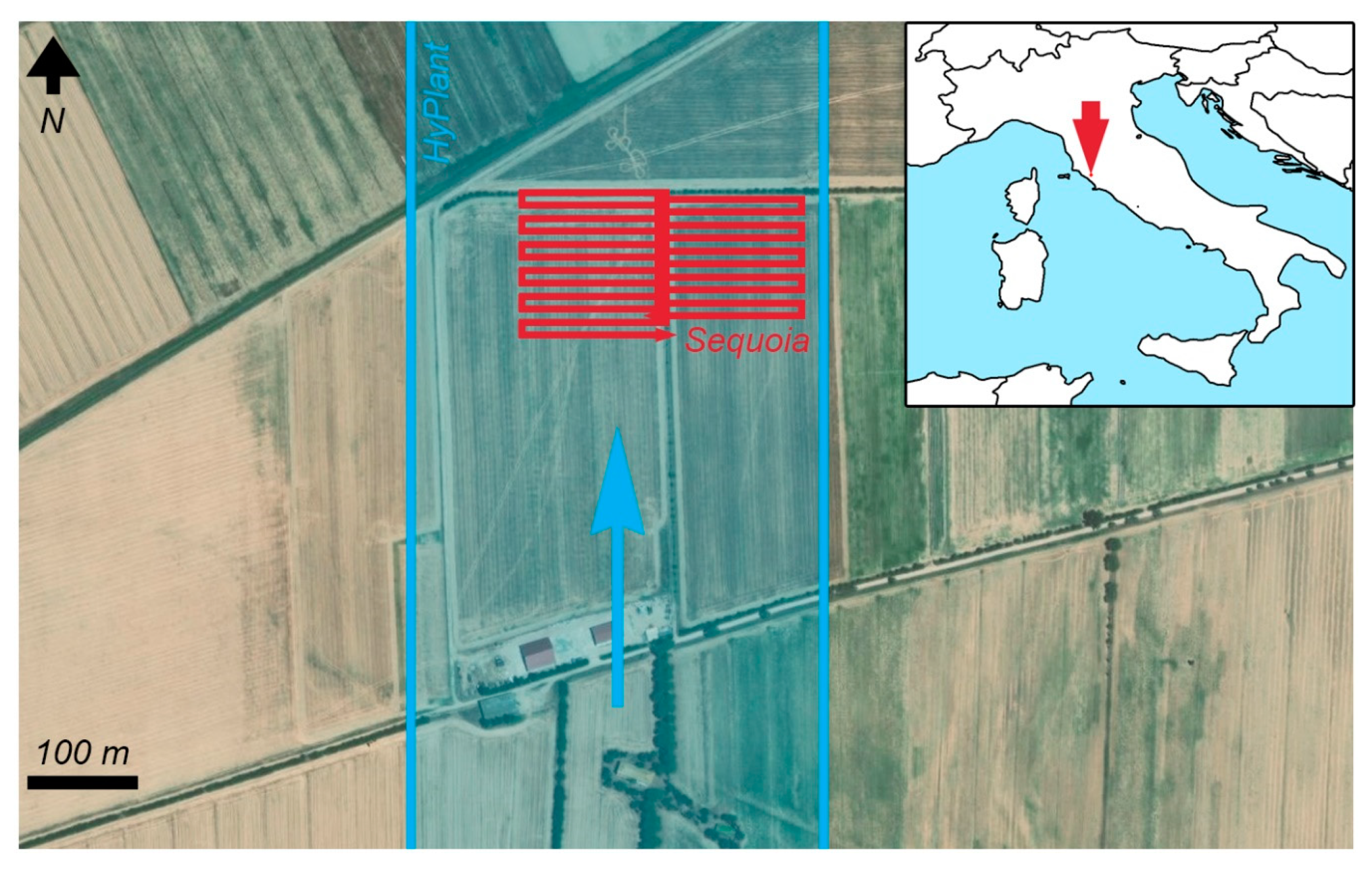
2.1. Study Site
2.2. Image Data
2.3. Field Measurements
2.3.1. Field Spectral Measurements for Calibration and Validation
2.3.2. Leaf Area Index Measurements
2.4. Image Data Processing
2.4.1. Surface Reflectance from Drone Image Data
2.4.2. Vegetation Index Products
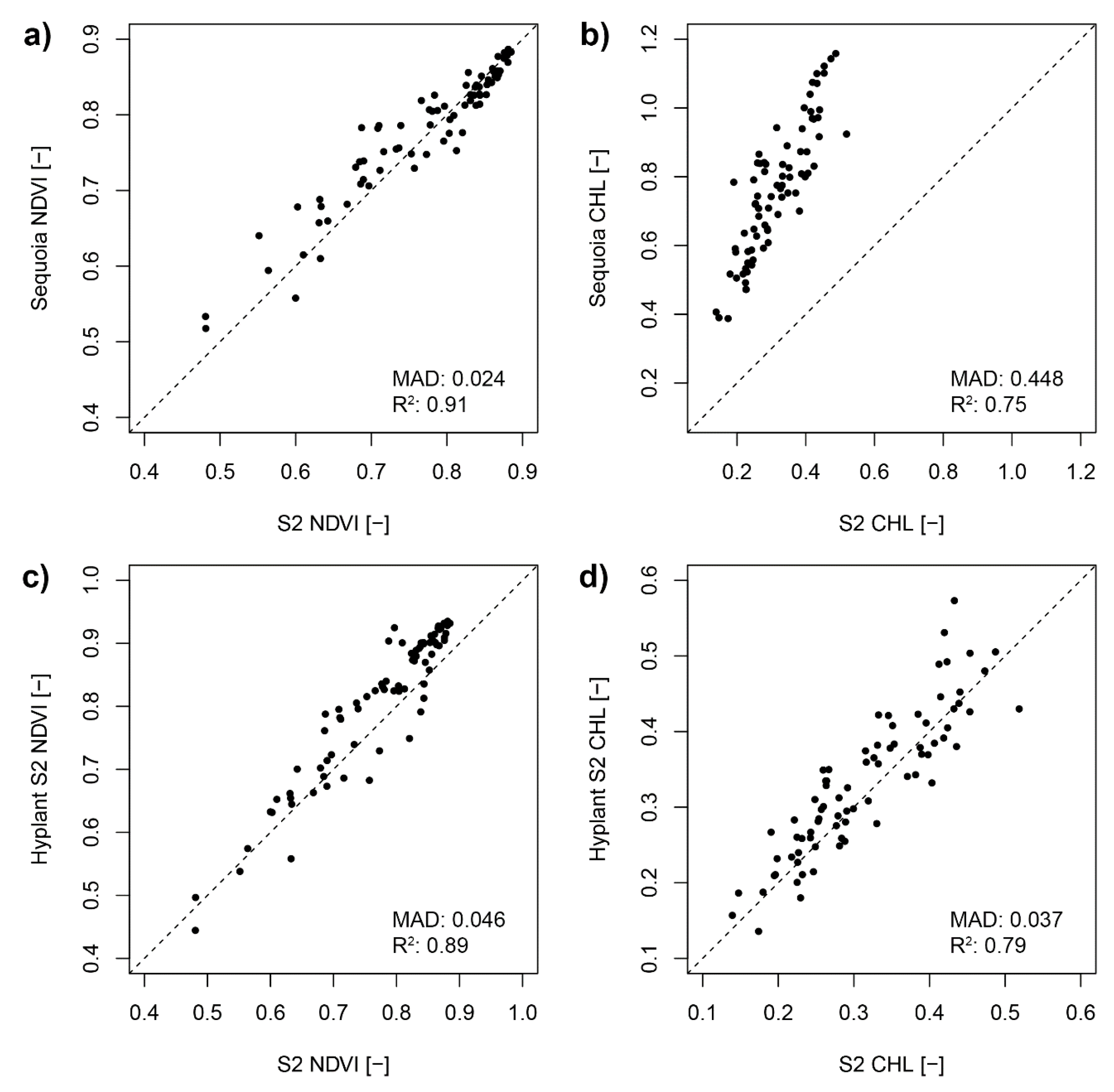
2.4.3. Multi-Scale HCRF and VI Intercomparison
3. Results
3.1. HCRF Products
3.1.1. Reference Target Validation of Drone Derived HCRF
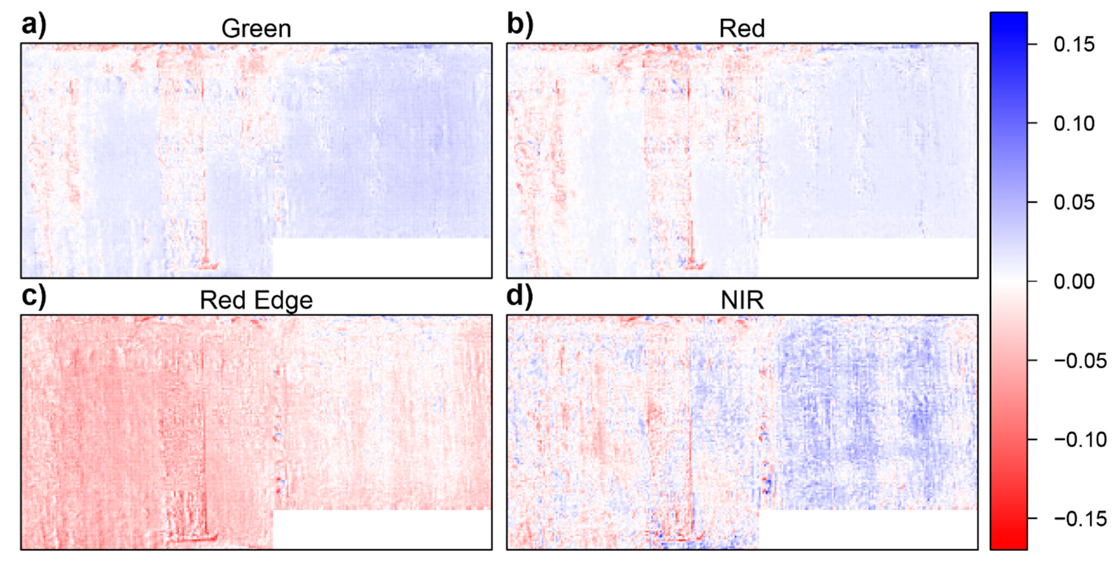
3.1.2. Spatial Comparison between Airborne and Drone Derived Surface Reflectance
3.2. Vegetation indices
4. Discussion
4.1. HCRF Accuracy
4.2. Multi-Scale VI Consistency and Sensitivity
5. Conclusions
Author Contributions
Funding
Acknowledgments
Conflicts of Interest
Appendix A. Simulations


| MAD between Sequoia Band Resampled Values and HyPlant to Sequoia Band Resampled Values | LAI Series (0.5–10) | Chlorophyll Content Series (0–100 µg/cm2) |
|---|---|---|
| Green | 0.0002 | 0.0001 |
| Red | 5.2631 × 10⁻⁶ | 1.6583 × 10⁻⁶ |
| Red edge | 0.0001 | 6.4832 × 10⁻⁵ |
| NIR | 5.7975 × 10⁻⁵ | 2.0239 × 10⁻⁵ |
References
- Gitelson, A.A.; Viña, A.; Ciganda, V.; Rundquist, D.C.; Arkebauer, T.J. Remote estimation of canopy chlorophyll content in crops. Geophys. Res. Lett. 2005, 32, 1–4. [Google Scholar] [CrossRef] [Green Version]
- Tucker, C.J.; Vanpraet, C.L.; Sharman, M.J.; Van Ittersum, G. Satellite remote sensing of total herbaceous biomass production in the senegalese sahel: 1980–1984. Remote Sens. Environ. 1985, 17, 233–249. [Google Scholar] [CrossRef]
- Gamon, J.A.; Somers, B.; Malenovský, Z.; Middleton, E.M.; Rascher, U.; Schaepman, M.E. Assessing Vegetation Function with Imaging Spectroscopy. Surv. Geophys. 2019, 40, 489–513. [Google Scholar] [CrossRef] [Green Version]
- Gamon, J.A. Reviews and Syntheses: Optical sampling of the flux tower footprint. Biogeosciences 2015, 12, 4509–4523. [Google Scholar] [CrossRef] [Green Version]
- Gamon, J.A.; Cheng, Y.; Claudio, H.; MacKinney, L.; Sims, D.A. A mobile tram system for systematic sampling of ecosystem optical properties. Remote Sens. Environ. 2006, 103, 246–254. [Google Scholar] [CrossRef]
- Hilker, T.; Coops, N.C.; Nesic, Z.; Wulder, M.A.; Black, A.T. Instrumentation and approach for unattended year round tower based measurements of spectral reflectance. Comput. Electron. Agric. 2007, 56, 72–84. [Google Scholar] [CrossRef]
- Anderson, K.; Gaston, K.J. Lightweight unmanned aerial vehicles will revolutionize spatial ecology. Front. Ecol. Environ. 2013, 11, 138–146. [Google Scholar] [CrossRef] [Green Version]
- Berni, J.A.J.; Zarco-Tejada, P.J.; Suárez, L.; Fereres, E. Thermal and narrowband multispectral remote sensing for vegetation monitoring from an unmanned aerial vehicle. IEEE Trans. Geosci. Remote Sens. 2009, 47, 722–738. [Google Scholar] [CrossRef] [Green Version]
- Garzonio, R.; di Mauro, B.; Colombo, R.; Cogliati, S. Surface reflectance and sun-induced fluorescence spectroscopy measurements using a small hyperspectral UAS. Remote Sens. 2017, 9, 472. [Google Scholar]
- Duffy, J.P.; Cunliffe, A.M.; DeBell, L.; Sandbrook, C.; Wich, S.A.; Shutler, J.D.; Myers-Smith, I.H.; Varela, M.R.; Anderson, K. Location, location, location: Considerations when using lightweight drones in challenging environments. Remote Sens. Ecol. Conserv. 2017, 4, 7–19. [Google Scholar] [CrossRef]
- Assmann, J.J.; Kerby, J.T.; Cunliffe, A.M.; Myers-smith, I.H. Vegetation monitoring using multispectral sensors—Best practices and lessons learned from high latitudes. J. Unmanned Veh. Syst. 2019, 7, 54–75. [Google Scholar] [CrossRef] [Green Version]
- Johansen, K.; Raharjo, T.; McCabe, M.F. Using multi-spectral UAV imagery to extract tree crop structural properties and assess pruning effects. Remote Sens. 2018, 10, 854. [Google Scholar] [CrossRef] [Green Version]
- Manuel Fernández-Guisuraga, J.; Sanz-Ablanedo, E.; Suárez-Seoane, S.; Calvo, L. Using Unmanned Aerial Vehicles in Postfire Vegetation Survey Campaigns through Large and Heterogeneous Areas: Opportunities and Challenges. Sensors 2018, 18, 586. [Google Scholar] [CrossRef] [PubMed] [Green Version]
- Nebiker, S.; Lack, N.; Abächerli, M.; Läderach, S. Light-weight multispectral uav sensors and their capabilities for predicting grain yield and detecting plant diseases. Int. Arch. Photogramm. Remote Sens. Spat. Inf. Sci. ISPRS Arch. 2016, 2016, 963–970. [Google Scholar] [CrossRef]
- Wang, S.; Garcia, M.; Ibrom, A.; Bauer-gottwein, P. Temporal interpolation of land surface fluxes derived from remote sensing—Results with an Unmanned Aerial System. Hydrol. Earth Syst. Sci. 2019, 1–27. [Google Scholar] [CrossRef] [Green Version]
- Kelcey, J.; Lucieer, A. Sensor correction of a 6-band multispectral imaging sensor for UAV remote sensing. Remote Sens. 2012, 4, 1462–1493. [Google Scholar] [CrossRef] [Green Version]
- Damm, A.; Guanter, L.; Verhoef, W.; Schläpfer, D.; Garbari, S.; Schaepman, M.E. Impact of varying irradiance on vegetation indices and chlorophyll fluorescence derived from spectroscopy data. Remote Sens. Environ. 2015, 156, 202–215. [Google Scholar] [CrossRef]
- Bendig, J.; Yu, K.; Aasen, H.; Bolten, A.; Bennertz, S.; Broscheit, J.; Gnyp, M.L.; Bareth, G. Combining UAV-based plant height from crop surface models, visible, and near infrared vegetation indices for biomass monitoring in barley. Int. J. Appl. Earth Obs. Geoinf. 2015, 39, 79–87. [Google Scholar] [CrossRef]
- Miura, T.; Huete, A.R.; Yoshioka, H. Evaluation of sensor calibration uncertainties on vegetation indices for MODIS. IEEE Trans. Geosci. Remote Sens. 2000, 38, 1399–1409. [Google Scholar] [CrossRef]
- Gevaert, C.M.; Suomalainen, J.; Tang, J.; Kooistra, L. Generation of Spectral-Temporal Response Surfaces by Combining Multispectral Satellite and Hyperspectral UAV Imagery for Precision Agriculture Applications. IEEE J. Sel. Top. Appl. Earth Obs. Remote Sens. 2015, 8, 3140–3146. [Google Scholar] [CrossRef]
- Van Leeuwen, W.J.D.; Orr, B.J.; Marsh, S.E.; Herrmann, S.M. Multi-sensor NDVI data continuity: Uncertainties and implications for vegetation monitoring applications. Remote Sens. Environ. 2006, 100, 67–81. [Google Scholar] [CrossRef]
- Easterday, K.; Kislik, C.; Dawson, T.; Hogan, S.; Kelly, M. Remotely Sensed Water Limitation in Vegetation: Insights from an Experiment with Unmanned Aerial Vehicles (UAVs). Remote Sens. 2019, 11, 1853. [Google Scholar] [CrossRef] [Green Version]
- Padró, J.C.; Muñoz, F.J.; Ávila, L.Á.; Pesquer, L.; Pons, X. Radiometric correction of Landsat-8 and Sentinel-2A scenes using drone imagery in synergy with field spectroradiometry. Remote Sens. 2018, 10, 1687. [Google Scholar] [CrossRef] [Green Version]
- Schaepman-Strub, G.; Schaepman, M.E.; Painter, T.H.; Dangel, S.; Martonchik, J.V. Reflectance quantities in optical remote sensing-definitions and case studies. Remote Sens. Environ. 2006, 103, 27–42. [Google Scholar] [CrossRef]
- Beck, H.E.; Zimmermann, N.E.; McVicar, T.R.; Vergopolan, N.; Berg, A.; Wood, E.F. Present and future köppen-geiger climate classification maps at 1-km resolution. Sci. Data 2018, 5, 1–12. [Google Scholar] [CrossRef] [Green Version]
- Rascher, U.; Alonso, L.; Burkart, A.; Cilia, C.; Cogliati, S.; Colombo, R.; Damm, A.; Drusch, M.; Guanter, L.; Hanus, J.; et al. Sun-induced fluorescence—A new probe of photosynthesis: First maps from the imaging spectrometer HyPlant. Glob. Chang. Biol. 2015, 21, 4673–4684. [Google Scholar] [CrossRef] [Green Version]
- Siegmann, B.; Alonso, L.; Celesti, M.; Cogliati, S.; Colombo, R.; Damm, A.; Douglas, S.; Guanter, L.; Hanuš, J.; Kataja, K.; et al. The high-performance airborne imaging spectrometer HyPlant—From raw images to top-of-canopy reflectance and fluorescence products: Introduction of an automatized processing chain. Remote Sens. 2019, 11, 2760. [Google Scholar] [CrossRef] [Green Version]
- Facchi, A.; Baroni, G.; Boschetti, M.; Gandolfi, C. Comparing Optical and Direct Methods for Leafarea Index Determination in a Maize Crop. J. Agric. Eng. 2010, 41, 33. [Google Scholar]
- Baret, F.; Weiss, M.; Allard, D.; Garrigues, S.; Leroy, M.; Jeanjean, H.; Fernandes, R.; Myneni, R.; Privette, J.; Morisette, J. VALERI: A network of sites and a methodology for the validation of medium spatial resolution land satellite products. Remote Sens. Environ. 2005, 76, 36–39. [Google Scholar]
- Parrot Parrot Sequoia Application Notes. Available online: https://forum.developer.parrot.com/t/parrot-announcement-release-of-application-notes/5455 (accessed on 2 February 2020).
- Fallet, C.; Domenzain, L.M. Necessary Steps for the Systematic Calibration of A Multispectral Imaging System to Achieve A Targetless Workflow in Reflectance Estimation: A Study of Parrot SEQUOIA for Precision Agriculture. In Proceedings of the Algorithms and Technologies for Multispectral, Hyperspectral, and Ultraspectral Imagery XXIV, Orlando, FL, USA, 17–19 April 2018; p. 42. [Google Scholar]
- Smith, G.M.; Milton, E.J. The use of the empirical line method to calibrate remotely sensed data to reflectance. Int. J. Remote Sens. 1999, 20, 2653–2662. [Google Scholar] [CrossRef]
- Jakob, S.; Zimmermann, R.; Gloaguen, R. The Need for Accurate Geometric and Radiometric Corrections of Drone-Borne Hyperspectral Data for Mineral Exploration: MEPHySTo—A Toolbox for Pre-Processing Drone-Borne Hyperspectral Data. Remote Sens. 2017, 9, 88. [Google Scholar] [CrossRef] [Green Version]
- Fawcett, D.; Anderson, K. Investigating Impacts of Calibration Methodology and Irradiance Variations on Lightweight Drone-Based Sensor Derived Surface Reflectance Products. In Proceedings of the Remote Sensing for Agriculture, Ecosystems, and Hydrology XXI, Strasbourg, France, 9–11 September 2019. [Google Scholar]
- Tu, Y.-H.; Phinn, S.; Johansen, K.; Robson, A. Assessing Radiometric Correction Approaches for Multi-Spectral UAS Imagery for Horticultural Applications. Remote Sens. 2018, 10, 1684. [Google Scholar] [CrossRef] [Green Version]
- Gitelson, A.A.; Wardlow, B.D.; Keydan, G.P.; Leavitt, B. An evaluation of MODIS 250-m data for green LAI estimation in crops. Geophys. Res. Lett. 2007, 34, 2–5. [Google Scholar] [CrossRef]
- D’Odorico, P.; Gonsamo, A.; Damm, A.; Schaepman, M.E. Experimental evaluation of sentinel-2 spectral response functions for NDVI time-series continuity. IEEE Trans. Geosci. Remote Sens. 2013, 51, 1336–1348. [Google Scholar] [CrossRef]
- Gilliot, J.-M.; Michelin, J.; Faroux, R.; Domenzain, L.M.; Fallet, C. Correction of in-flight luminosity variations in multispectral UAS images, using a luminosity sensor and camera pair for improved biomass estimation in precision agriculture. Proc. SPIE Int. Soc. Opt. Eng. 2018, 10664, 1066405. [Google Scholar]
- Stow, D.; Nichol, C.J.; Wade, T.; Assmann, J.J.; Simpson, G.; Helfter, C. Illumination Geometry and Flying Height Influence Surface Reflectance and NDVI Derived from Multispectral UAS Imagery. Drones 2019, 3, 55. [Google Scholar] [CrossRef] [Green Version]
- Ji, H.; Wang, K. Robust image deblurring with an inaccurate blur kernel. IEEE Trans. Image Process. 2012, 21, 1624–1634. [Google Scholar] [CrossRef]
- Adler, K. Radiometric Correction of Multispectral Images Collected by A UAV for Phenology Studies; Lund University: Lund, Sweden, 2018. [Google Scholar]
- Hakala, T.; Markelin, L.; Honkavaara, E.; Scott, B.; Theocharous, T.; Nevalainen, O.; Näsi, R.; Suomalainen, J.; Viljanen, N.; Greenwell, C.; et al. Direct reflectance measurements from drones: Sensor absolute radiometric calibration and system tests for forest reflectance characterization. Sensors 2018, 18, 1417. [Google Scholar] [CrossRef] [Green Version]
- Thome, K.; Smith, N.; Scott, K. Vicarious Calibration of MODIS Using Railroad Valley Playa. In Proceedings of the International Geoscience and Remote Sensing Symposium (IGARSS), IEEE, Yokohama, Japan, 9–13 July 2001; Volume 3, pp. 1209–1211. [Google Scholar]
- Revill, A.; Florence, A.; MacArthur, A.; Hoad, S.; Rees, R.; Williams, M. The Value of Sentinel-2 Spectral Bands for the Assessment of Winter Wheat Growth and Development. Remote Sens. 2019, 11, 2050. [Google Scholar] [CrossRef] [Green Version]
- Aasen, H.; Bolten, A. Multi-temporal high-resolution imaging spectroscopy with hyperspectral 2D imagers – From theory to application. Remote Sens. Environ. 2018, 205, 374–389. [Google Scholar] [CrossRef]
- Hakala, T.; Suomalainen, J.; Peltoniemi, J.I. Acquisition of bidirectional reflectance factor dataset using a micro unmanned aerial vehicle and a consumer camera. Remote Sens. 2010, 2, 819–832. [Google Scholar] [CrossRef] [Green Version]
- Román, M.O.; Gatebe, C.K.; Schaaf, C.B.; Poudyal, R.; Wang, Z.; King, M.D. Variability in surface BRDF at different spatial scales (30 m–500 m) over a mixed agricultural landscape as retrieved from airborne and satellite spectral measurements. Remote Sens. Environ. 2011, 115, 2184–2203. [Google Scholar] [CrossRef] [Green Version]
- Toulios, L.; Dercas, N.; Psomiadis, E.; Kavvadias, A.; Chanioti, M.; Tsitouras, A. Unmanned Aerial Vehicle (UAV) Data Analysis for Fertilization Dose Assessment. In Proceedings of the Remote Sensing for Agriculture, Ecosystems, and Hydrology XIX, Warsaw, Poland, 12–14 September 2017; Volume 1042121, p. 78. [Google Scholar]
- Berra, E.F.; Gaulton, R.; Barr, S. Assessing spring phenology of a temperate woodland: A multiscale comparison of ground, unmanned aerial vehicle and Landsat satellite observations. Remote Sens. Environ. 2019, 223, 229–242. [Google Scholar] [CrossRef]
- Matese, A.; Toscano, P.; Di Gennaro, S.F.; Genesio, L.; Vaccari, F.P.; Primicerio, J.; Belli, C.; Zaldei, A.; Bianconi, R.; Gioli, B. Intercomparison of UAV, aircraft and satellite remote sensing platforms for precision viticulture. Remote Sens. 2015, 7, 2971–2990. [Google Scholar] [CrossRef] [Green Version]
- Hakala, T.; Honkavaara, E.; Saari, H.; Mäkynen, J.; Kaivosoja, J.; Pesonen, L.; Pölönen, I. Spectral Imaging From Uavs Under Varying Illumination Conditions. ISPRS Int. Arch. Photogramm. Remote Sens. Spat. Inf. Sci. 2013, XL-1/W2, 189–194. [Google Scholar] [CrossRef] [Green Version]
- Jacquemoud, S.; Verhoef, W.; Baret, F.; Bacour, C.; Zarco-Tejada, P.J.; Asner, G.P.; François, C.; Ustin, S.L. PROSPECT + SAIL models: A review of use for vegetation characterization. Remote Sens. Environ. 2009, 113, S56–S66. [Google Scholar] [CrossRef]
- Atzberger, C.; Richter, K. Spatially constrained inversion of radiative transfer models for improved LAI mapping from future Sentinel-2 imagery. Remote Sens. Environ. 2012, 120, 208–218. [Google Scholar] [CrossRef]


| Dataset Descriptor | Sensor | Acquisition Time | Ground Sampling Distance (GSD) | Bandwidth | Spectral Range |
|---|---|---|---|---|---|
| Sequoia A1 | Parrot Sequoia | 6th July 2018 16:07 (UTC+2) | 4.15 cm | 10–40 nm | 550–790 nm |
| Sequoia A2 (F2A + F2B) | Parrot Sequoia | 7th July 2018 11:50 to 12:20 (UTC+2) | 4.71 cm | 10–40 nm | 550–790 nm |
| HyPlant | HyPlant dual-channel module | 7th July 2018 12:32 (UTC+2) | 1 m | 3–4 nm | 380–2500 nm |
| S2 | Sentinel 2A MultiSpectral Instrument | 8th July 2018 12:10 (UTC+2) | 20 m | 18–45 nm | 440–2200 nm |
| Calibration Method | MAD Green | MAD Red | MAD Red Edge | MAD NIR |
|---|---|---|---|---|
| Single panel calibration | 0.029 (13.63% *) | 0.023 (11.11% *) | 0.019 (7.53% *) | 0.033 (11.95% *) |
| ELM with 0 intercept | 0.02 (9.69% *) | 0.027 (13.18% *) | 0.023 (8.76% *) | 0.027 (11.21% *) |
| ELM with modified 0 intercept | 0.009 (4.19% *) | 0.025 (12.29% *) | 0.02 (8.87% *) | 0.036 (14.75% *) |
| Calibration Method | MAD Green | MAD Red | MAD Red Edge | MAD NIR |
|---|---|---|---|---|
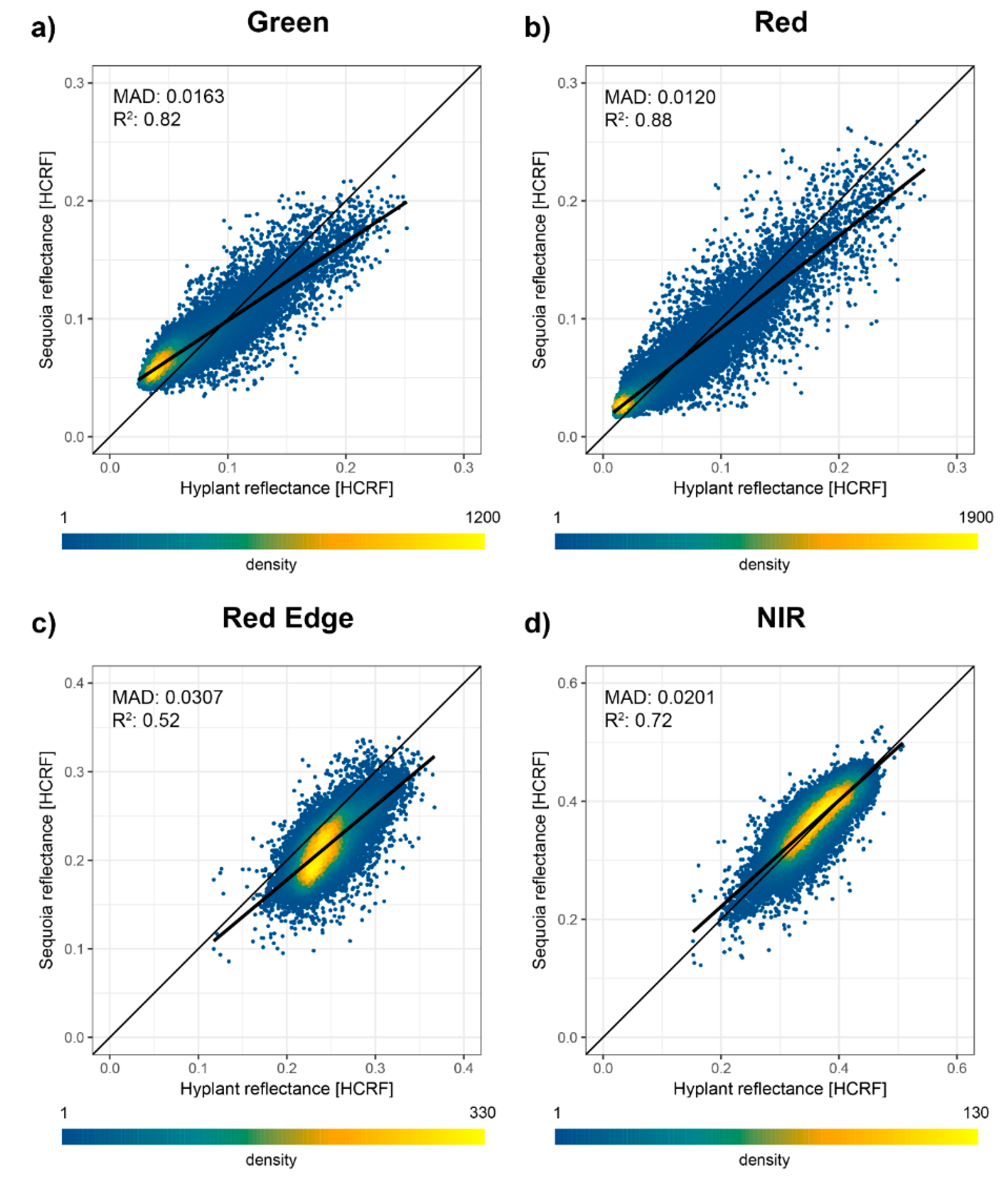
| Single panel calibration | 0.0163 (25.39% *) | 0.0120 (26.10% *) | 0.0307 (12.56% *) | 0.0201 (5.61% *) |
| ELM, 0 intercept | 0.0177 (27.58% *) | 0.0117 (25.45% *) | 0.0194 (7.94% *) | 0.0360 (10.05% *) |
| ELM, modified 0 intercept | 0.0118 (18.38% *) | 0.0110 (23.93% *) | 0.0539 (22.05% *) | 0.0479 (13.37% *) |
| Validation Surface | Error Green | Error Red | Error Red Edge | Error NIR |
|---|---|---|---|---|
| 0.05 HCRF (Black) | 0.0044 (9.61% *) | 0.0045 (10.19% *) | 0.0036 (7.95% *) | 0.0038 (8.35% *) |
| 0.4 HCRF (Grey) | 0.0097 (2.20% *) | 0.0071 (1.62% *) | 0.0017 (0.39% *) | 0.0001 (0.03% *) |
| 0.7 HCRF (White) | −0.0181 (−2.53% *) | −0.0155 (−2.22% *) | −0.0178 (−2.58% *) | −0.0152 (−2.24% *) |
| Calibration Method | MAD NDVI | MAD CHL |
|---|---|---|
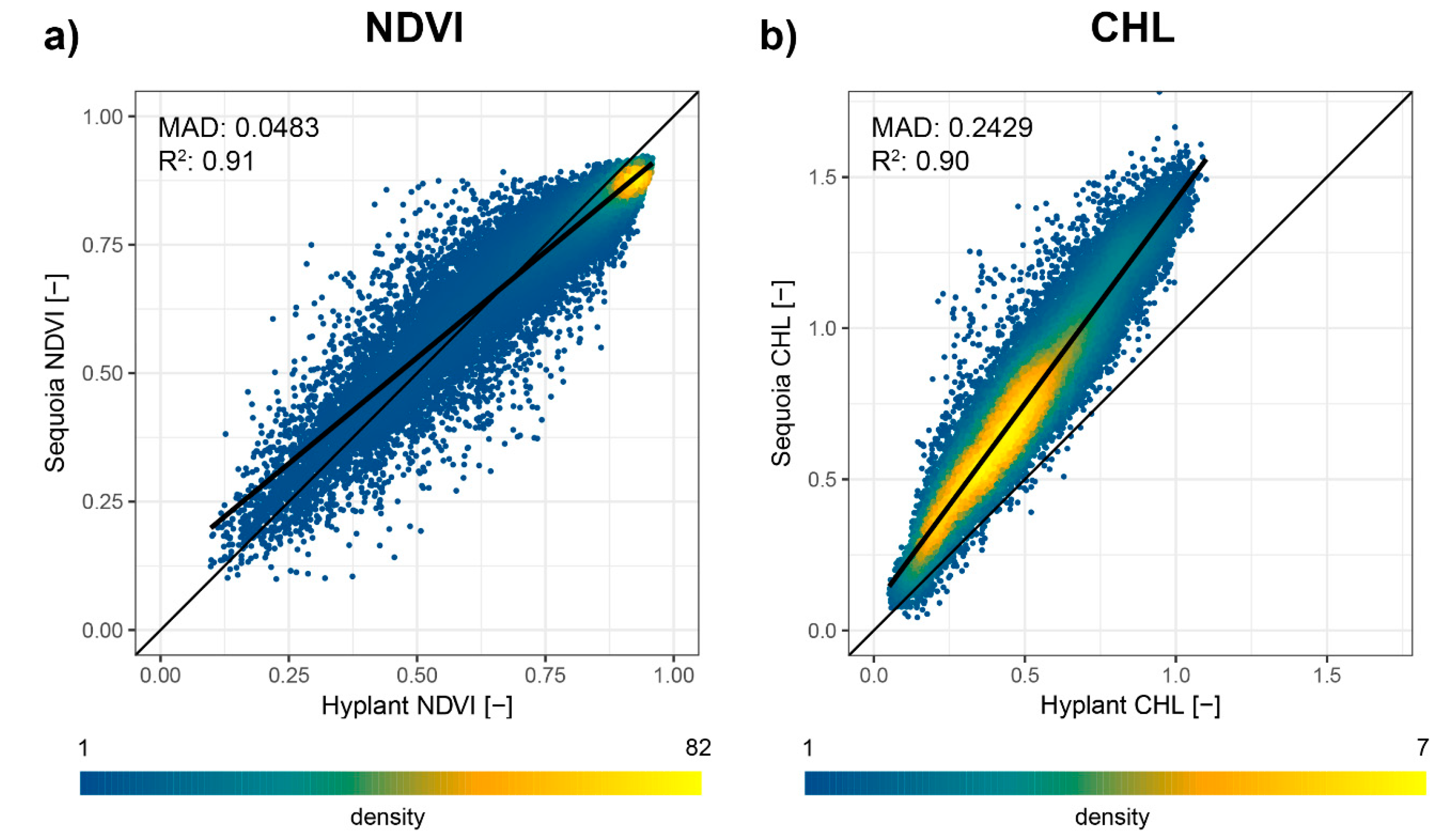
| Single panel calibration | 0.0483 (6.20% *) | 0.2429 (50.97% *) |
| ELM, 0 intercept | 0.0468 (6.01% *) | 0.2227 (46.73% *) |
| ELM, 0 intercept, minimum subtracted | 0.0387 (4.97% *) | 0.2069 (43.42% *) |
© 2020 by the authors. Licensee MDPI, Basel, Switzerland. This article is an open access article distributed under the terms and conditions of the Creative Commons Attribution (CC BY) license (http://creativecommons.org/licenses/by/4.0/).
Share and Cite
Fawcett, D.; Panigada, C.; Tagliabue, G.; Boschetti, M.; Celesti, M.; Evdokimov, A.; Biriukova, K.; Colombo, R.; Miglietta, F.; Rascher, U.; et al. Multi-Scale Evaluation of Drone-Based Multispectral Surface Reflectance and Vegetation Indices in Operational Conditions. Remote Sens. 2020, 12, 514. https://0-doi-org.brum.beds.ac.uk/10.3390/rs12030514
Fawcett D, Panigada C, Tagliabue G, Boschetti M, Celesti M, Evdokimov A, Biriukova K, Colombo R, Miglietta F, Rascher U, et al. Multi-Scale Evaluation of Drone-Based Multispectral Surface Reflectance and Vegetation Indices in Operational Conditions. Remote Sensing. 2020; 12(3):514. https://0-doi-org.brum.beds.ac.uk/10.3390/rs12030514
Chicago/Turabian StyleFawcett, Dominic, Cinzia Panigada, Giulia Tagliabue, Mirco Boschetti, Marco Celesti, Anton Evdokimov, Khelvi Biriukova, Roberto Colombo, Franco Miglietta, Uwe Rascher, and et al. 2020. "Multi-Scale Evaluation of Drone-Based Multispectral Surface Reflectance and Vegetation Indices in Operational Conditions" Remote Sensing 12, no. 3: 514. https://0-doi-org.brum.beds.ac.uk/10.3390/rs12030514