Statistical Applications to Downscale GRACE-Derived Terrestrial Water Storage Data and to Fill Temporal Gaps

 ,
,  , , ,
, , ,
Abstract
:
1. Introduction
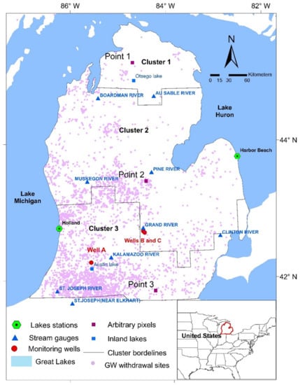
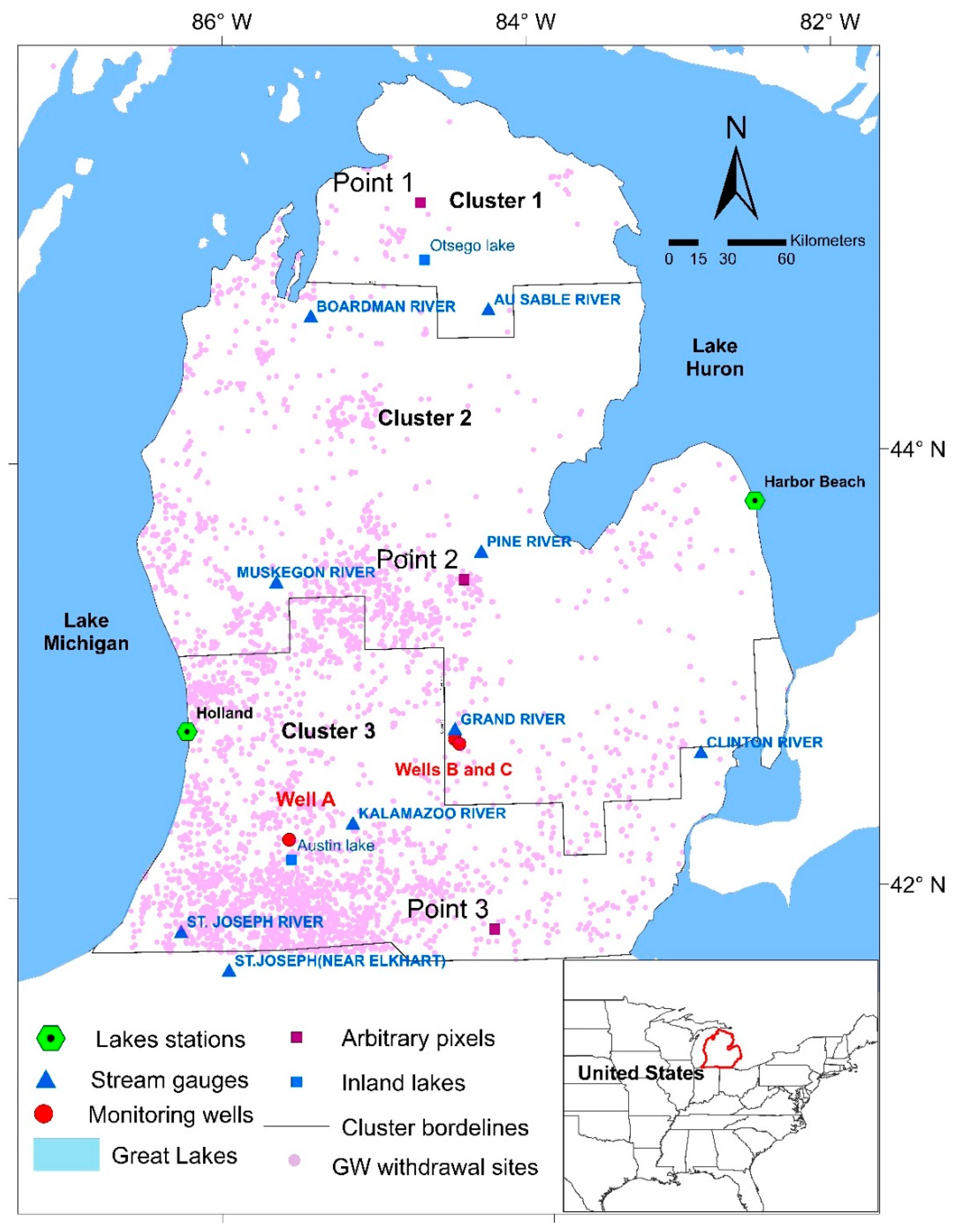
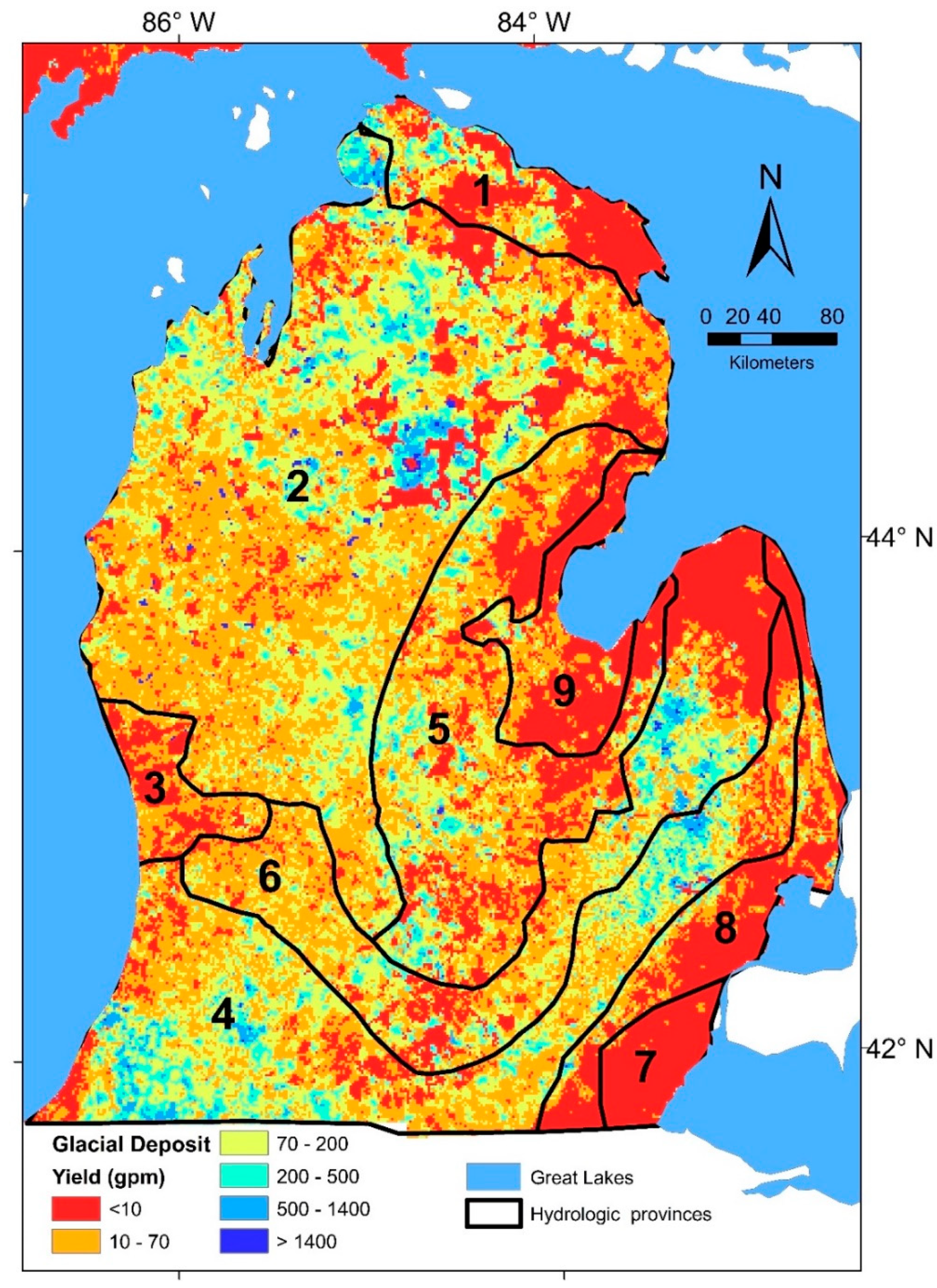
2. Overview of the Study Area
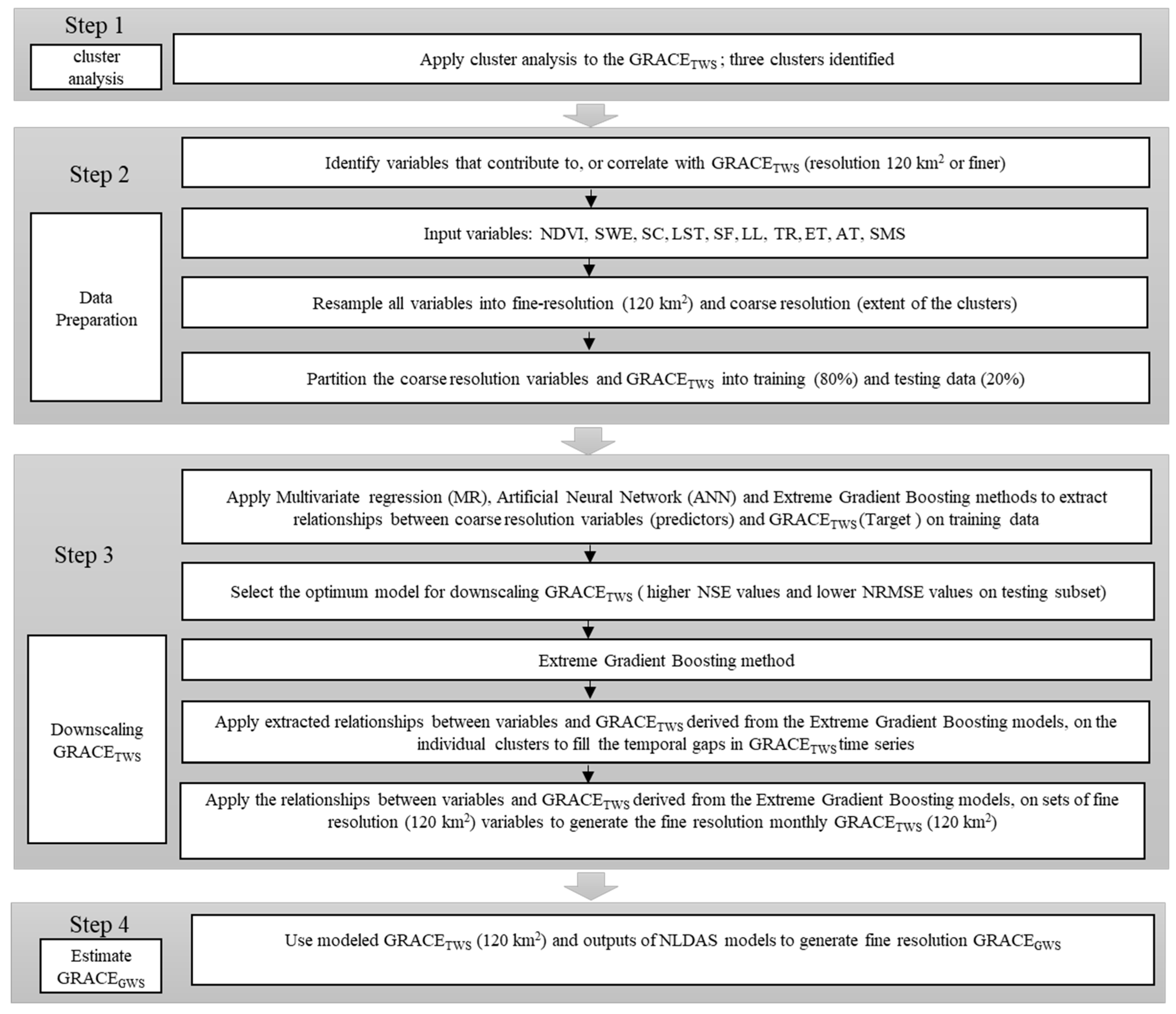
3. Methodology
3.1. Cluster Analysis
3.2. Identification of Variables that Correlate with and/or Control GRACETWS
3.2.1. GRACE-Derived TWS
3.2.2. NDVI
3.2.3. Snow Cover (SC)
3.2.4. Stream Flow (SF)
3.2.5. Lake Levels (LL)
3.2.6. Land Surface Temperature (LST)
3.2.7. Rainfall, Snow Water Equivalent, Soil Moisture, Air Temperature, and Evapotranspiration
3.3. Construction, Evaluation, and Selection of an Optimum Model for Downscaling
3.3.1. MR Models
3.3.2. ANN
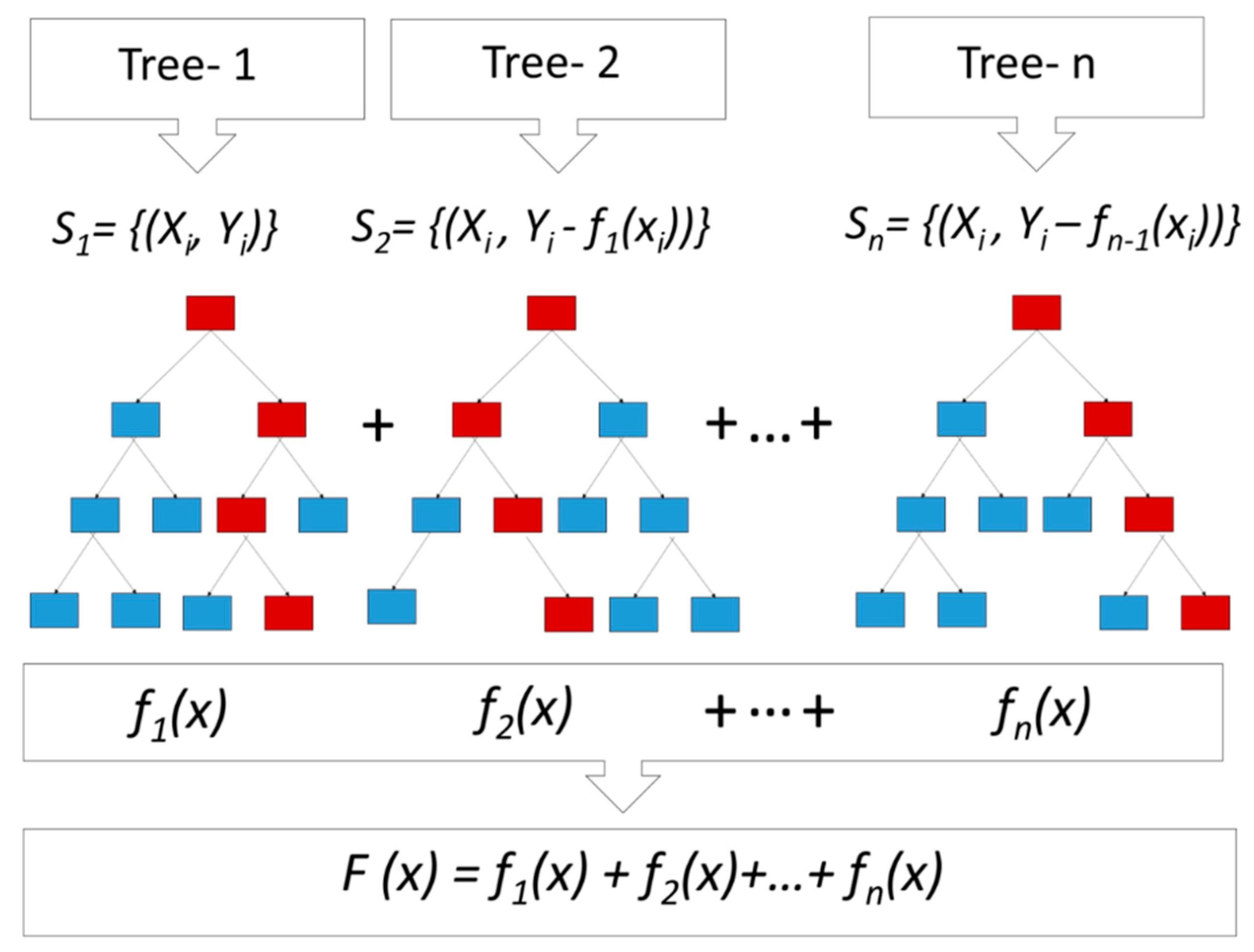
3.3.3. XGBoost
- Calculate the negative gradients of J with respect to F(Xi), which is .
- Fit a regression tree, , to negative gradients .
- Let our new F(Xi) be F(Xi) + , where is the step size in our algorithm to reach the estimated minimum of .
3.3.4. Selection of Optimum Statistical Model and Gap Filling
3.4. Extraction of Temporal Groundwater Storage Using Outputs of Land Surface Models
Sources and Propagation of Errors
4. Results
4.1. Cluster Analysis
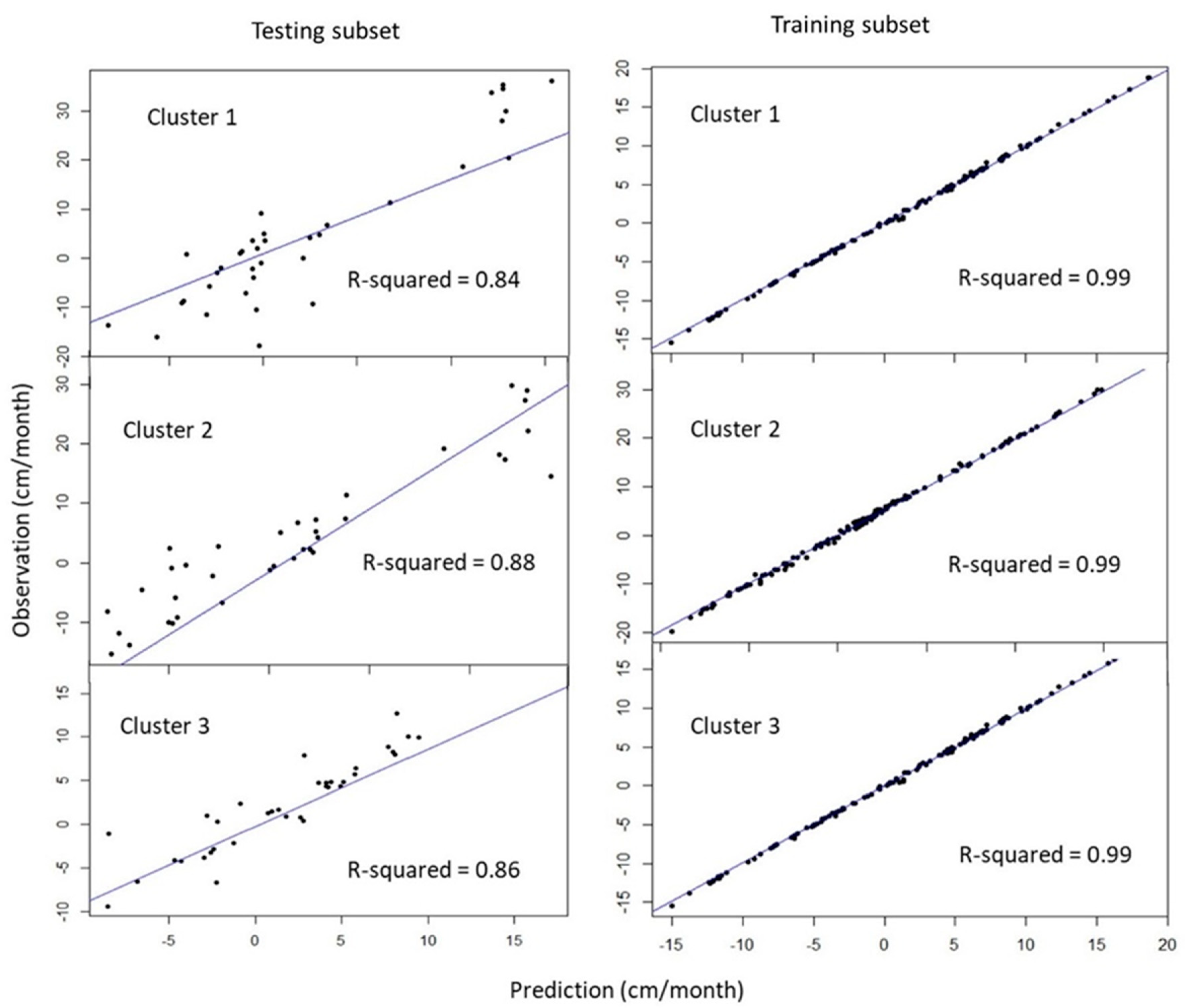
4.2. Evaluation and Comparison of the Models
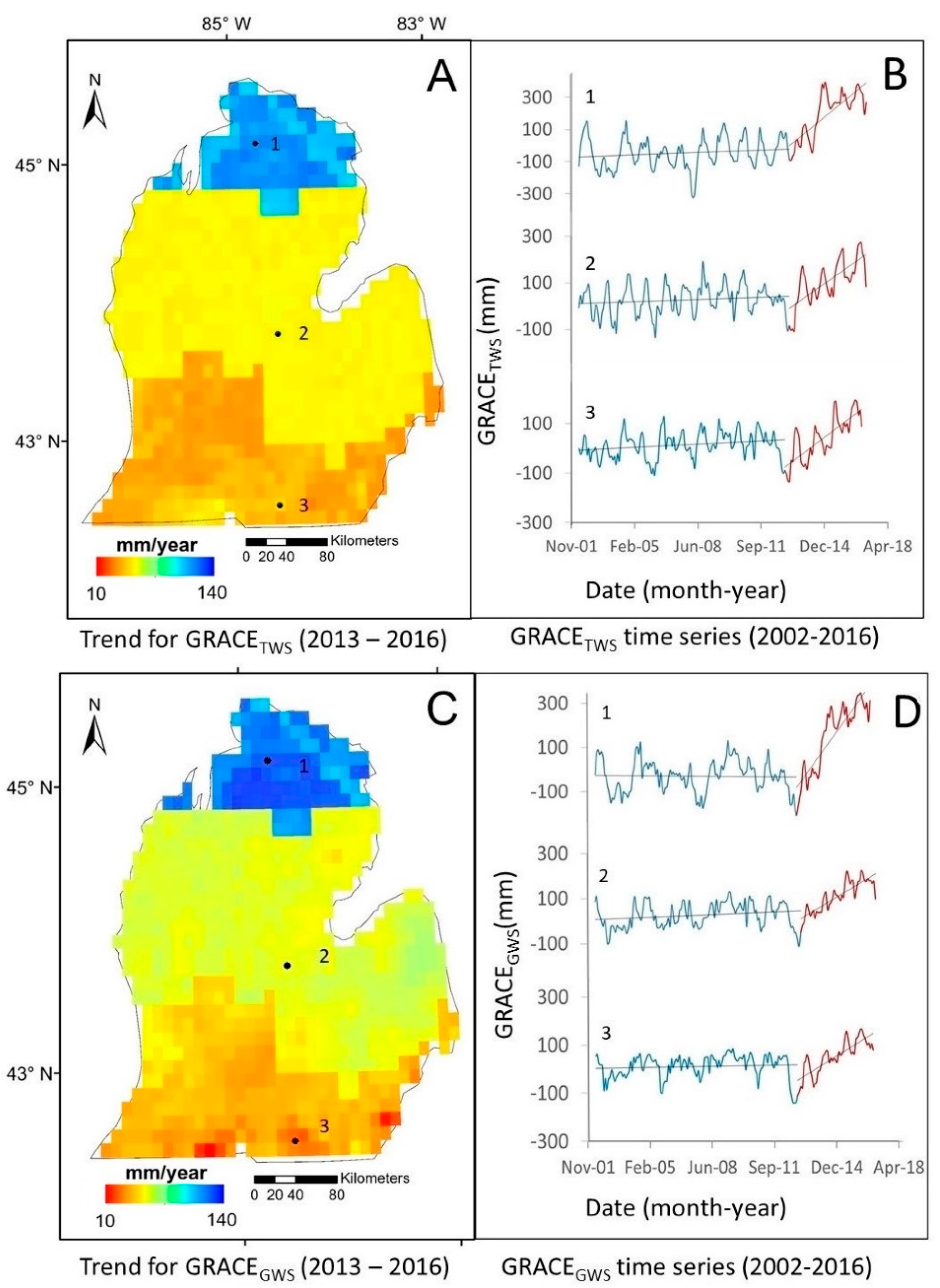
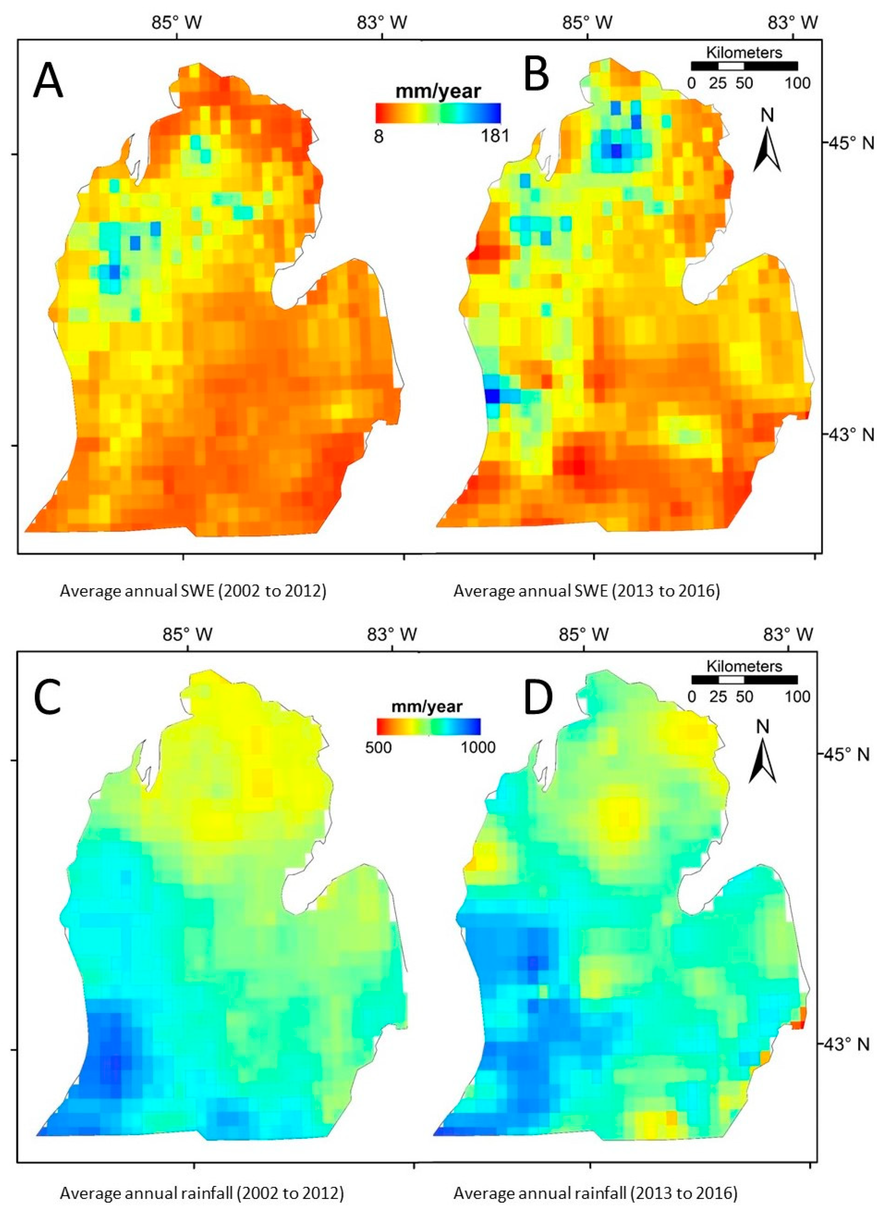
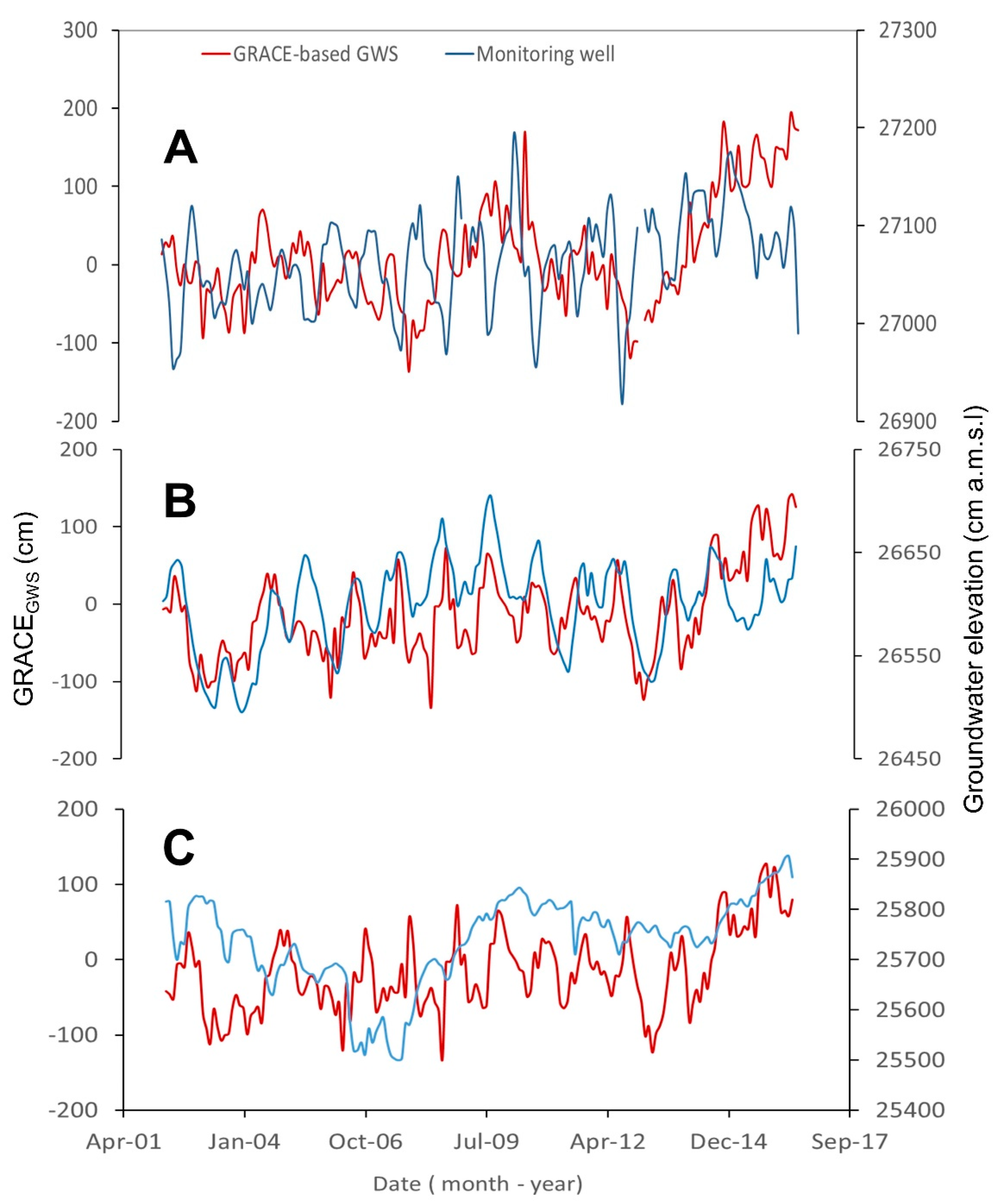
4.3. Factors Controlling the TWS and GWS Variations over the Study Area
5. Discussion
6. Conclusions
Author Contributions
Funding
Conflicts of Interest
References
- Tapley, B.D.; Bettadpur, S.; Ries, J.C.; Thompson, P.F.; Watkins, M.M. GRACE measurements of mass variability in the earth system. Science 2004, 305, 503–505. [Google Scholar] [CrossRef] [PubMed] [Green Version]
- Tapley, B.D.; Bettadpur, S.; Watkins, M.; Reigber, C. The Gravity Recovery and Climate Experiment: Mission Overview and Early Results. Geophys. Res. Lett. 2004, 31, L09607. [Google Scholar] [CrossRef] [Green Version]
- Ahmed, M.; Sultan, M.; Wahr, J.; Yan, E. The Use of GRACE Data to Monitor Natural and Anthropogenic Induced Variations in Water Availability across Africa. Earth-Sci. Rev. 2014, 136, 289–300. [Google Scholar] [CrossRef]
- Abdelmohsen, K.; Sultan, M.; Ahmed, M.; Save, H.; Elkaliouby, B.; Emil, M.; Yan, E.; Abotalib, A.Z.; Krishnamurthy, R.V.; Abdelmalik, K. Response of Deep Aquifers to Climate Variability. Sci. Total Environ. 2019, 677, 530–544. [Google Scholar] [CrossRef]
- Abdelmalik, K.W.; Abdelmohsen, K. GRACE and TRMM Mission: The Role of Remote Sensing Techniques for Monitoring Spatio-Temporal Change in Total Water Mass, Nile Basin. J. Afr. Earth Sci. 2019, 160. [Google Scholar] [CrossRef]
- Othman, A.; Sultan, M.; Becker, R.; Alsefry, S.; Alharbi, T.; Gebremichael, E.; Alharbi, H.; Abdelmohsen, K. Use of Geophysical and Remote Sensing Data for Assessment of Aquifer Depletion and Related Land Deformation. Surv. Geophys. 2018, 39, 543–566. [Google Scholar] [CrossRef] [Green Version]
- Sultan, M.; Sturchio, N.C.; Alsefry, S.; Emil, M.K.; Ahmed, M.; Abdelmohsen, K.; AbuAbdullah, M.M.; Yan, E.; Save, H.; Alharbi, T.; et al. Assessment of Age, Origin, and Sustainability of Fossil Aquifers: A Geochemical and Remote Sensing-Based Approach. J. Hydrol. 2019, 576, 325–341. [Google Scholar] [CrossRef]
- Feng, W.; Zhong, M.; Lemoine, J.-M.; Biancale, R.; Hsu, H.-T.; Xia, J. Evaluation of Groundwater Depletion in North China Using the Gravity Recovery and Climate Experiment (GRACE) Data and Ground-Based Measurements. Water Resour. Res. 2013, 49, 2110–2118. [Google Scholar] [CrossRef]
- Rodell, M.; Velicogna, I.; Famiglietti, J.S. Satellite-Based Estimates of Groundwater Depletion in India. Nature 2009, 460, 999–1002. [Google Scholar] [CrossRef] [Green Version]
- Scanlon, B.R.; Longuevergne, L.; Long, D. Ground Referencing GRACE Satellite Estimates of Groundwater Storage Changes in the California Central Valley, USA. Water Resour. Res. 2012, 48, W04520. [Google Scholar] [CrossRef] [Green Version]
- Castellazzi, P.; Longuevergne, L.; Martel, R.; Rivera, A.; Brouard, C.; Chaussard, E. Quantitative Mapping of Groundwater Depletion at the Water Management Scale Using a Combined GRACE/InSAR Approach. Remote Sens. Environ. 2018, 205, 408–418. [Google Scholar] [CrossRef]
- Wahr, J.; Swenson, S.; Zlotnicki, V.; Velicogna, I. Time-Variable Gravity from GRACE: First Results. Geophys. Res. Lett. 2004, 31, L11501. [Google Scholar] [CrossRef] [Green Version]
- Wahr, J.; Swenson, S.; Velicogna, I. Accuracy of GRACE Mass Estimates. Geophys. Res. Lett. 2006, 33, L06401. [Google Scholar] [CrossRef] [Green Version]
- Rodell, M.; Houser, P.R.; Jambor, U.; Gottschalck, J.; Mitchell, K.; Meng, C.-J.; Arsenault, K.; Cosgrove, B.; Radakovich, J.; Bosilovich, M.; et al. The Global Land Data Assimilation System. Bull. Am. Meteorol. Soc. 2004, 85, 381–394. [Google Scholar] [CrossRef] [Green Version]
- Chen, J.L.; Rodell, M.; Wilson, C.R.; Famiglietti, J.S. Low Degree Spherical Harmonic Influences on Gravity Recovery and Climate Experiment (GRACE) Water Storage Estimates. Geophys. Res. Lett. 2005, 32, L14405. [Google Scholar] [CrossRef] [Green Version]
- Atkinson, P.M. Downscaling in Remote Sensing. Int. J. Appl. Earth Obs. Geoinf. 2013, 22, 106–114. [Google Scholar] [CrossRef]
- Zaitchik, B.F.; Rodell, M.; Reichle, R.H.; Zaitchik, B.F.; Rodell, M.; Reichle, R.H. Assimilation of GRACE Terrestrial Water Storage Data into a Land Surface Model: Results for the Mississippi River Basin. J. Hydrometeorol. 2008, 9, 535–548. [Google Scholar] [CrossRef]
- Houborg, R.; Rodell, M.; Li, B.; Reichle, R.; Zaitchik, B.F. Drought Indicators Based on Model-Assimilated Gravity Recovery and Climate Experiment (GRACE) Terrestrial Water Storage Observations. Water Resour. Res. 2012, 48, W07525. [Google Scholar] [CrossRef] [Green Version]
- Sahoo, A.K.; De Lannoy, G.J.M.; Reichle, R.H.; Houser, P.R. Assimilation and Downscaling of Satellite Observed Soil Moisture over the Little River Experimental Watershed in Georgia, USA. Adv. Water Resour. 2013, 52, 19–33. [Google Scholar] [CrossRef]
- Shokri, A.; Walker, J.P.; Dijk, A.I.J.M.; Pauwels, V.R.N. On the Use of Adaptive Ensemble Kalman Filtering to Mitigate Error Misspecifications in GRACE Data Assimilation. Water Resour. Res. 2019, 55, 7622–7637. [Google Scholar] [CrossRef] [Green Version]
- Shokri, A.; Walker, J.P.; Dijk, A.I.J.M.; Pauwels, V.R.N. Performance of Different Ensemble Kalman Filter Structures to Assimilate GRACE Terrestrial Water Storage Estimates Into a High-Resolution Hydrological Model: A Synthetic Study. Water Resour. Res. 2018, 54, 8931–8951. [Google Scholar] [CrossRef]
- Landerer, F.W.; Swenson, S.C. Accuracy of Scaled GRACE Terrestrial Water Storage Estimates. Water Resour. Res. 2012, 48, W04531. [Google Scholar] [CrossRef]
- Schoof, J.T. Statistical Downscaling in Climatology. Geogr. Compass 2013, 7, 249–265. [Google Scholar] [CrossRef] [Green Version]
- Le Roux, R.; Katurji, M.; Zawar-Reza, P.; Quénol, H.; Sturman, A. Comparison of Statistical and Dynamical Downscaling Results from the WRF Model. Environ. Model. Softw. 2018, 100, 67–73. [Google Scholar] [CrossRef]
- Hou, Y.-K.; Chen, H.; Xu, C.-Y.; Chen, J.; Guo, S.-L.; Hou, Y.-K.; Chen, H.; Xu, C.-Y.; Chen, J.; Guo, S.-L. Coupling a Markov Chain and Support Vector Machine for At-Site Downscaling of Daily Precipitation. J. Hydrometeorol. 2017, 18, 2385–2406. [Google Scholar] [CrossRef] [Green Version]
- Jin, Y.; Ge, Y.; Wang, J.; Heuvelink, G.; Wang, L. Geographically Weighted Area-to-Point Regression Kriging for Spatial Downscaling in Remote Sensing. Remote Sens. 2018, 10, 579. [Google Scholar] [CrossRef] [Green Version]
- Miro, M.; Famiglietti, J. Downscaling GRACE Remote Sensing Datasets to High-Resolution Groundwater Storage Change Maps of California’s Central Valley. Remote Sens. 2018, 10, 143. [Google Scholar] [CrossRef] [Green Version]
- So, B.-J.; Kim, J.-Y.; Kwon, H.-H.; Lima, C.H.R. Stochastic Extreme Downscaling Model for an Assessment of Changes in Rainfall Intensity-Duration-Frequency Curves over South Korea Using Multiple Regional Climate Models. J. Hydrol. 2017, 553, 321–337. [Google Scholar] [CrossRef]
- Joshi, D.; St-Hilaire, A.; Ouarda, T.; Daigle, A. Statistical Downscaling of Precipitation and Temperature Using Sparse Bayesian Learning, Multiple Linear Regression and Genetic Programming Frameworks. Can. Water Resour. J./Rev. Can. Des Ressour. Hydr. 2015, 40, 392–408. [Google Scholar] [CrossRef]
- Ezzine, H.; Bouziane, A.; Ouazar, D.; Hasnaoui, M.D. Downscaling of TRMM3B43 Product Through Spatial and Statistical Analysis Based on Normalized Difference Water Index, Elevation, and Distance From Sea. IEEE Geosci. Remote Sens. Lett. 2017, 14, 1449–1453. [Google Scholar] [CrossRef]
- Chadwick, R.; Coppola, E.; Giorgi, F. An Artificial Neural Network Technique for Downscaling GCM Outputs to RCM Spatial Scale. Nonlinear Process. Geophys. 2011, 18, 1013–1028. [Google Scholar] [CrossRef]
- Vu, M.T.; Aribarg, T.; Supratid, S.; Raghavan, S.V.; Liong, S.-Y. Statistical Downscaling Rainfall Using Artificial Neural Network: Significantly Wetter Bangkok? Theor. Appl. Climatol. 2016, 126, 453–467. [Google Scholar] [CrossRef]
- Sun, A.Y. Predicting Groundwater Level Changes Using GRACE Data. Water Resour. Res. 2013, 49, 5900–5912. [Google Scholar] [CrossRef]
- Yin, W.; Hu, L.; Zhang, M.; Wang, J.; Han, S.-C. Statistical Downscaling of GRACE-Derived Groundwater Storage Using ET Data in the North China Plain. J. Geophys. Res. Atmos. 2018, 123, 5973–5987. [Google Scholar] [CrossRef]
- Seyoum, W.; Kwon, D.; Milewski, A. Downscaling GRACE TWSA Data into High-Resolution Groundwater Level Anomaly Using Machine Learning-Based Models in a Glacial Aquifer System. Remote Sens. 2019, 11, 824. [Google Scholar] [CrossRef] [Green Version]
- Tayyebi, A.; Smidt, S.; Pijanowski, B. Long-Term Land Cover Data for the Lower Peninsula of Michigan, 2010–2050. Data 2017, 2, 16. [Google Scholar] [CrossRef] [Green Version]
- Census Bureau, U. Income, Poverty, and Health Insurance Coverage in the United States. 2009. Available online: https://www.census.gov/prod/2010pubs/p60-238.pdf (accessed on 15 November 2019).
- Grannemann, N.G.; Hunt, R.J.; Nicholas, J.R.; Reilly, T.E.; Winter, T.C. The Importance of Ground Water in the Great Lakes Region; Water-Resources Investigations Report 00–4008; US Geological Survey: Reston, VA, USA, 2000.
- Rheaume, S.J. Hydrologic Provinces of Michigan; Water-Resources Investigations Report 91–4120; US Geological Survey: Lansing, MI, USA, 1991.
- Vugrinovich, R. Patterns of Regional Subsurface Fluid Movement in the Michigan Basin. Available online: https://www.michigan.gov/documents/deq/GIMDL-OFR866_302614_7.pdf (accessed on 15 November 2019).
- Groundwater Inventory and Mapping Project Summary and Status—September. 2004. Available online: http://mrwa.org/wp-content/uploads/repository/Exec_Summ_Final_081805.pdf (accessed on 15 November 2019).
- Dhanachandra, N.; Manglem, K.; Chanu, Y.J. Image Segmentation Using K-Means Clustering Algorithm and Subtractive Clustering Algorithm. Procedia Comput. Sci. 2015, 54, 764–771. [Google Scholar] [CrossRef] [Green Version]
- Tibshirani, R.; Walther, G.; Hastie, T. Estimating the Number of Clusters in a Data Set via the Gap Statistic. J. R. Stat. Soc. Ser. B (Stat. Methodol.) 2001, 63, 411–423. [Google Scholar] [CrossRef]
- Save, H.; Bettadpur, S.; Tapley, B.D. High-Resolution CSR GRACE RL05 Mascons. J. Geophys. Res. Solid Earth 2016, 121, 7547–7569. [Google Scholar] [CrossRef]
- Save, H.; Bettadpur, S.; Tapley, B.D. Reducing Errors in the GRACE Gravity Solutions Using Regularization. J. Geod. 2012, 86, 695–711. [Google Scholar] [CrossRef]
- Watkins, M.M.; Wiese, D.N.; Yuan, D.N.; Boening, C.; Landerer, F.W. Improved Methods for Observing Earth’s Time Variable Mass Distribution with GRACE Using Spherical Cap Mascons. J. Geophys. Res. B Solid Earth 2015, 120, 2648–2671. [Google Scholar] [CrossRef]
- Luthcke, S.B.; Sabaka, T.J.; Loomis, B.D.; Arendt, A.A.; McCarthy, J.J.; Camp, J. Antarctica, Greenland and Gulf of Alaska Land-Ice Evolution from an Iterated GRACE Global Mascon Solution. J. Glaciol. 2013, 59, 613–631. [Google Scholar] [CrossRef]
- Rodell, M.; Famiglietti, J.S.; Wiese, D.N.; Reager, J.T.; Beaudoing, H.K.; Landerer, F.W.; Lo, M.H. Emerging Trends in Global Freshwater Availability. Nature 2018, 557, 651–659. [Google Scholar] [CrossRef] [PubMed]
- Scanlon, B.R.; Zhang, Z.; Save, H.; Sun, A.Y.; Schmied, H.M.; Van Beek, L.P.H.; Wiese, D.N.; Wada, Y.; Long, D.; Reedy, R.C.; et al. Global Models Underestimate Large Decadal Declining and Rising Water Storage Trends Relative to GRACE Satellite Data. Proc. Natl. Acad. Sci. USA 2018, 115, E1080–E1089. [Google Scholar] [CrossRef] [Green Version]
- Luthcke, S.B.; Rowlands, D.D.; Lemoine, F.G.; Klosko, S.M.; Chinn, D.; McCarthy, J.J. Monthly Spherical Harmonic Gravity Field Solutions Determined from GRACE Inter-Satellite Range-Rate Data Alone. Geophys. Res. Lett. 2006, 33, L02402. [Google Scholar] [CrossRef]
- Ahmed, M.; Sultan, M.; Wahr, J.; Yan, E.; Milewski, A.; Sauck, W.; Becker, R.; Welton, B. Integration of GRACE (Gravity Recovery and Climate Experiment) Data with Traditional Data Sets for a Better Understanding of the Time-Dependent Water Partitioning in African Watersheds. Geology 2011, 39, 479–482. [Google Scholar] [CrossRef] [Green Version]
- Scanlon, B.R.; Zhang, Z.; Save, H.; Wiese, D.N.; Landerer, F.W.; Long, D.; Longuevergne, L.; Chen, J. Global Evaluation of New GRACE Mascon Products for Hydrologic Applications. Water Resour. Res. 2016, 52, 9412–9429. [Google Scholar] [CrossRef]
- Ahmed, M.; Abdelmohsen, K. Quantifying Modern Recharge and Depletion Rates of the Nubian Aquifer in Egypt. Surv. Geophys. 2018, 39, 729–751. [Google Scholar] [CrossRef]
- The Land Processes Distributed Active Archive Center. Available online: https://lpdaac.usgs.gov/data/ (accessed on 15 November 2019).
- Van Leeuwen, W.J.D.; Orr, B.J.; Marsh, S.E.; Herrmann, S.M. Multi-Sensor NDVI Data Continuity: Uncertainties and Implications for Vegetation Monitoring Applications. Remote Sens. Environ. 2006, 100, 67–81. [Google Scholar] [CrossRef]
- National Snow and Ice Data Center. Available online: https://nsidc.org/ (accessed on 15 November 2019).
- Frappart, F.; Ramillien, G.; Ronchail, J. Changes in Terrestrial Water Storage versus Rainfall and Discharges in the Amazon Basin. Int. J. Climatol. 2013, 33, 3029–3046. [Google Scholar] [CrossRef] [Green Version]
- Prakash, S.; Gairola, R.M.; Papa, F.; Mitra, A.K. An Assessment of Terrestrial Water Storage, Rainfall and River Discharge over Northern India from Satellite Data. Curr. Sci. 2014, 107, 1582–1586. [Google Scholar] [CrossRef]
- Nikzad Tehrani, E.; Sahour, H.; Booij, M.J. Trend Analysis of Hydro-Climatic Variables in the North of Iran. Theor. Appl. Climatol. 2019, 136, 85–97. [Google Scholar] [CrossRef]
- USGS Current Conditions for Michigan_Streamflow. Available online: https://waterdata.usgs.gov/mi/nwis/current/?type=flow (accessed on 15 November 2019).
- NOAA Tides and Currents. Available online: https://tidesandcurrents.noaa.gov/ (accessed on 15 November 2019).
- MODIS/Aqua Land-Surface Temperature/Emissivity Monthly Global 0.05Deg CMG-LAADS DAAC. Available online: https://ladsweb.modaps.eosdis.nasa.gov/missions-and-measurements/products/MYD11C3/ (accessed on 15 November 2019).
- Wang, W.; Liang, S.; Meyers, T. Validating MODIS Land Surface Temperature Products Using Long-Term Nighttime Ground Measurements. Remote Sens. Environ. 2008, 112, 623–635. [Google Scholar] [CrossRef]
- Mitchell, K.E.; Lohmann, D.; Houser, P.R.; Wood, E.F.; Schaake, J.C.; Robock, A.; Cosgrove, B.A.; Sheffield, J.; Duan, Q.; Luo, L.; et al. The Multi-institution North American Land Data Assimilation System (NLDAS): Utilizing Multiple GCIP Products and Partners in a Continental Distributed Hydrological Modeling System. J. Geophys. Res. Atmos. 2004, 109, D07S90. [Google Scholar] [CrossRef] [Green Version]
- NASA- GES DISC. Available online: https://disc.gsfc.nasa.gov/datasets?keywords=NLDAS (accessed on 15 November 2019).
- Xu, T.; Guo, Z.; Xia, Y.; Ferreira, V.G.; Liu, S.; Wang, K.; Yao, Y.; Zhang, X.; Zhao, C. Evaluation of Twelve Evapotranspiration Products from Machine Learning, Remote Sensing and Land Surface Models over Conterminous United States. J. Hydrol. 2019, 578, 124105. [Google Scholar] [CrossRef]
- Xia, Y.; Mitchell, K.; Ek, M.; Sheffield, J.; Cosgrove, B.; Wood, E.; Luo, L.; Alonge, C.; Wei, H.; Meng, J.; et al. Continental-Scale Water and Energy Flux Analysis and Validation for the North American Land Data Assimilation System Project Phase 2 (NLDAS-2): 1. Intercomparison and Application of Model Products. J. Geophys. Res. Atmos. 2012, 117, D03109. [Google Scholar] [CrossRef]
- Xia, Y.; Mitchell, K.; Ek, M.; Cosgrove, B.; Sheffield, J.; Luo, L.; Alonge, C.; Wei, H.; Meng, J.; Livneh, B.; et al. Continental-Scale Water and Energy Flux Analysis and Validation for North American Land Data Assimilation System Project Phase 2 (NLDAS-2): 2. Validation of Model-Simulated Streamflow. J. Geophys. Res. Atmos. 2012, 117, D03110. [Google Scholar] [CrossRef]
- Xia, Y.; Sheffield, J.; Ek, M.B.; Dong, J.; Chaney, N.; Wei, H.; Meng, J.; Wood, E.F. Evaluation of Multi-Model Simulated Soil Moisture in NLDAS-2. J. Hydrol. 2014, 512, 107–125. [Google Scholar] [CrossRef]
- Sheffield, J.; Pan, M.; Wood, E.F.; Mitchell, K.E.; Houser, P.R.; Schaake, J.C.; Robock, A.; Lohmann, D.; Cosgrove, B.; Duan, Q.; et al. Snow Process Modeling in the North American Land Data Assimilation System (NLDAS): 1. Evaluation of Model-simulated Snow Cover Extent. J. Geophys. Res. Atmos. 2003, 108. [Google Scholar] [CrossRef] [Green Version]
- Mo, K.C.; Chen, L.-C.; Shukla, S.; Bohn, T.J.; Lettenmaier, D.P. Uncertainties in North American Land Data Assimilation Systems over the Contiguous United States. J. Hydrometeorol. 2012, 13, 996–1009. [Google Scholar] [CrossRef]
- Henn, B.; Newman, A.J.; Livneh, B.; Daly, C.; Lundquist, J.D. An Assessment of Differences in Gridded Precipitation Datasets in Complex Terrain. J. Hydrol. 2018, 556, 1205–1219. [Google Scholar] [CrossRef]
- Nash, J.E.; Sutcliffe, J.V. River Flow Forecasting through Conceptual Models Part I—A Discussion of Principles. J. Hydrol. 1970, 10, 282–290. [Google Scholar] [CrossRef]
- Moriasi, D.N.; Arnold, J.G.; Van Liew, M.W.; Bingner, R.L.; Harmel, R.D.; Veith, T.L. Model Evaluation Guidelines for Systematic Quantification of Accuracy in Watershed Simulations. Trans. ASABE 2007, 50, 885–900. [Google Scholar] [CrossRef]
- Hocking, R.R. A Biometrics Invited Paper. The Analysis and Selection of Variables in Linear Regression. Biometrics 1976, 32, 1. [Google Scholar] [CrossRef]
- Zolfaghari, A.; Izadi, M. Burst Pressure Prediction of Cylindrical Vessels Using Artificial Neural Network. J. Press. Vessel Technol. 2019, PVT-19-1142. [Google Scholar] [CrossRef]
- Gholami, V.; Booij, M.J.; Nikzad Tehrani, E.; Hadian, M.A. Spatial Soil Erosion Estimation Using an Artificial Neural Network (ANN) and Field Plot Data. Catena 2018, 163, 210–218. [Google Scholar] [CrossRef]
- Mohaghegi, S.; Del Valle, Y.; Venayagamoorthy, G.K.; Harley, R.G. A Comparison of PSO and Backpropagation for Training RBF Neural Networks for Identification of a Power System with Statcom. In Proceedings of the 2005 IEEE Swarm Intelligence Symposium, Pasadena, CA, USA, 8–10 June 2005; pp. 391–394. [Google Scholar]
- Rumelhart, D.E.; Hinton, G.E.; Williams, R.J. Learning Representations by Back-Propagating Errors. Nature 1986, 323, 533–536. [Google Scholar] [CrossRef]
- De’ath, G. Boosted Trees for Ecological Modeling and Prediction. Ecology 2007, 88, 243–251. [Google Scholar] [CrossRef]
- Friedman, J.H. Greedy Function Approximation: A Gradient Boosting Machine. Ann. Stat. 2001, 29, 1189–1232. [Google Scholar] [CrossRef]
- Mason, L.; Bartlett, P.; Baxter, J.; Frean, M. Boosting Algorithms as Gradient Descent. In Advances in Neural Information Processing Systems 12; MIT Press: Cambridge, MA, USA, 2000; p. 1098. [Google Scholar]
- Chen, T.; Guestrin, C. XGBoost: A Scalable Tree Boosting System. In Proceedings of the 22nd ACM SIGKDD International Conference on Knowledge Discovery and Data Mining, New York, NY, USA, 13–17 August 2016; pp. 785–794. [Google Scholar]
- Castle, S.L.; Thomas, B.F.; Reager, J.T.; Rodell, M.; Swenson, S.C.; Famiglietti, J.S. Groundwater Depletion during Drought Threatens Future Water Security of the Colorado River Basin. Geophys. Res. Lett. 2014, 41, 5904–5911. [Google Scholar] [CrossRef] [Green Version]
- Voss, K.A.; Famiglietti, J.S.; Lo, M.; de Linage, C.; Rodell, M.; Swenson, S.C. Groundwater Depletion in the Middle East from GRACE with Implications for Transboundary Water Management in the Tigris-Euphrates-Western Iran Region. Water Resour. Res. 2013, 49, 904–914. [Google Scholar] [CrossRef] [PubMed] [Green Version]
- Fisher, R.A. Statistical Methods for Research Workers; Springer: New York, NY, USA, 1992; pp. 66–70. [Google Scholar] [CrossRef]
- Alin, A. Multicollinearity. Wiley Interdiscip. Rev. Comput. Stat. 2010, 2, 370–374. [Google Scholar] [CrossRef]
- Gronewold, A.D.; Bruxer, J.; Durnford, D.; Smith, J.P.; Clites, A.H.; Seglenieks, F.; Qian, S.S.; Hunter, T.S.; Fortin, V. Hydrological Drivers of Record-Setting Water Level Rise on Earth’s Largest Lake System. Water Resour. Res. 2016, 52, 4026–4042. [Google Scholar] [CrossRef] [Green Version]
- Andersen, T.; Carstensen, J.; Hernández-García, E.; Duarte, C.M. Ecological Thresholds and Regime Shifts: Approaches to Identification. Trends Ecol. Evol. 2009, 24, 49–57. [Google Scholar] [CrossRef] [Green Version]
- Krabbenhoft, D.P.; Bowser, C.J.; Anderson, M.P.; Valley, J.W. Estimating Groundwater Exchange with Lakes: 1. The Stable Isotope Mass Balance Method. Water Resour. Res. 1990, 26, 2445–2453. [Google Scholar] [CrossRef]
- Krabbenhoft, D.P.; Webster, K.E. Transient Hydrogeological Controls on the Chemistry of a Seepage Lake. Water Resour. Res. 1995, 31, 2295–2305. [Google Scholar] [CrossRef]
- Wiese, D.; Argus, D.; Yuan, D.; Landerer, F. Combining satellite gravimetry and in-situ GNSS measurements to improve spatial resolution of mass flux estimates. In Proceedings of the GRACE Science Team Meeting (GSTM), Pasadena, CA, USA, 8–10 October 2019. [Google Scholar]


| Variable Name | Format | Resolution | Source |
|---|---|---|---|
| NDVI | raster | (0.05° × 0.05°) | MODIS |
| Snow cover | raster | (0.05° × 0.05°) | MODIS |
| Land surface temperature | raster | (0.05° × 0.05°) | MODIS |
| Total precipitation | raster | (0.125° × 0.125°) | NLDAS |
| Air temperature | raster | (0.125° × 0.125°) | NLDAS |
| Soil moisture | raster | (0.125° × 0.125°) | NLDAS |
| Lakes Level | numerical | N/A | NOAA |
| Streamflow | numerical | N/A | USGS |
| Evapotranspiration | raster | (0.125° × 0.125°) | NLDAS |
| Cluster | ΔTWS (mm/year) | ΔSMS (mm/year) | ΔSWE (mm/year) | ΔGWS (mm/year) |
|---|---|---|---|---|
| 1 | 16.2 ± 5 | 0.3 ± 0.0 | 0.1 ± 0.0 | 15.8 ± 5 |
| 2 | 14.4 ± 5.2 | 0.0 ± 0.0 | 0.7 ± 0.0 | 13.7 ± 5.2 |
| 3 | 8.8 ± 3.4 | −0.7 ± 0.0 | 0.1 ± 0.0 | 9.5 ± 3.4 |
| Performance Rating | NSE | NRMSE |
|---|---|---|
| Very Good | NSE ≥ 0.75 | NRMSE ≤ 0.5 |
| Good | NSE ≥ 0.65 and < 0.75 | NRMSE > 0.50 and ≤ 0.60 |
| Satisfactory | NSE ≥ 0.50 and < 0.65 | NRMSE > 0.60 and ≤ 0.70 |
| Unsatisfactory | NSE < 0.5 | NRMSE > 0.70 |
| Method | Cluster 1 | Cluster 2 | Cluster 3 | ||||
|---|---|---|---|---|---|---|---|
| Coefficients | Uncertainty (%) | Coefficients | Uncertainty (%) | Coefficients | Uncertainty (%) | ||
| Extreme Gradient Boosting | R-squared | 0.84 | 16 | 0.88 | 12 | 0.86 | 14 |
| NSE | 0.84 | 16 | 0.87 | 13 | 0.85 | 15 | |
| NRMSE | 0.4 | 40 | 0.35 | 35 | 0.38 | 38 | |
| Average Uncertainty (%) | 24 | 20 | 22.3 | ||||
| Ranking * | VG | VG | VG | ||||
| Artificial Neural Networks | R-squared | 0.6 | 40 | 0.84 | 16 | 0.86 | 16 |
| NSE | 0.25 | 75 | 0.84 | 16 | 0.82 | 18 | |
| NRMSE | 0.85 | 85 | 0.4 | 40 | 0.42 | 42 | |
| Average Uncertainty (%) | 66.7 | 24 | 25.3 | ||||
| Ranking | US | VG | VG | ||||
| Multivariate Regression | R-squared | 0.72 | 28 | 0.76 | 24 | 0.85 | 15 |
| NSE | 0.6 | 4 | 0.75 | 25 | 0.83 | 17 | |
| NRMSE | 0.62 | 62 | 0.48 | 48 | 0.4 | 40 | |
| Average Uncertainty (%) | 31.3 | 32.3 | 24 | ||||
| Ranking * | S | VG | VG | ||||
| Cluster1 | Cluster2 | Cluster3 | Lake Level | |
|---|---|---|---|---|
| Cluster1 | 1 | |||
| Cluster2 | 0.41 | 1 | ||
| Cluster3 | 0.66 | 0.56 | 1 | |
| Lake Level | 0.74 | 0.43 | 0.58 | 1 |
| Variables | |||||||
|---|---|---|---|---|---|---|---|
| Clusters | Total Precipitation | Temperature | NDVI | Soil Moisture | Lake Michigan Level | Streamflow | Evapotranspiration |
| 1 | 5.1 (1) * | 1.4 | 2.2 (1) | 13.3 (2) | 69.6 (1) | 6.1 (1) | 1.3 (2) |
| 2 | 3.1 (3) | 1.4 (3) | 0.00 | 1.6 (1) | 68.6 (2) | 23.0 (1) | 1.6 (2) |
| 3 | 3.7 (1) | 0.00 | 3.6 (2) | 38.7 (1) | 48.1 (2) | 5.9 | 0.0 |
© 2020 by the authors. Licensee MDPI, Basel, Switzerland. This article is an open access article distributed under the terms and conditions of the Creative Commons Attribution (CC BY) license (http://creativecommons.org/licenses/by/4.0/).
Share and Cite
Sahour, H.; Sultan, M.; Vazifedan, M.; Abdelmohsen, K.; Karki, S.; Yellich, J.A.; Gebremichael, E.; Alshehri, F.; Elbayoumi, T.M. Statistical Applications to Downscale GRACE-Derived Terrestrial Water Storage Data and to Fill Temporal Gaps. Remote Sens. 2020, 12, 533. https://0-doi-org.brum.beds.ac.uk/10.3390/rs12030533
Sahour H, Sultan M, Vazifedan M, Abdelmohsen K, Karki S, Yellich JA, Gebremichael E, Alshehri F, Elbayoumi TM. Statistical Applications to Downscale GRACE-Derived Terrestrial Water Storage Data and to Fill Temporal Gaps. Remote Sensing. 2020; 12(3):533. https://0-doi-org.brum.beds.ac.uk/10.3390/rs12030533
Chicago/Turabian StyleSahour, Hossein, Mohamed Sultan, Mehdi Vazifedan, Karem Abdelmohsen, Sita Karki, John A. Yellich, Esayas Gebremichael, Fahad Alshehri, and Tamer M. Elbayoumi. 2020. "Statistical Applications to Downscale GRACE-Derived Terrestrial Water Storage Data and to Fill Temporal Gaps" Remote Sensing 12, no. 3: 533. https://0-doi-org.brum.beds.ac.uk/10.3390/rs12030533