Optimized Segmentation Based on the Weighted Aggregation Method for Loess Bank Gully Mapping

Abstract

The Chinese Loess Plateau suffers severe gully erosion. Gully mapping is a fundamental task for gully erosion monitoring in this region. Among the different gully types in the Loess Plateau, the bank gully is usually regarded as the most important source for the generation of sediment. However, approaches for bank gully extraction are still limited. This study put forward an integrated framework, including segmentation optimization, evaluation and Extreme Gradient Boosting (XGBoost)-based classification, for the bank gully mapping of Zhifanggou catchment in the Chinese Loess Plateau. The approach was conducted using a 1-m resolution digital elevation model (DEM), based on unmanned aerial vehicle (UAV) photogrammetry and WorldView-3 imagery. The methodology first divided the study area into different watersheds. Then, segmentation by weighted aggregation (SWA) was implemented to generate multi-level segments. For achieving an optimum segmentation, area-weighted variance (WV) and Moran’s I (MI) were adopted and calculated within each sub-watershed. After that, a new discrepancy metric, the area-number index (ANI), was developed for evaluating the segmentation results, and the results were compared with the multi-resolution segmentation (MRS) algorithm. Finally, bank gully mappings were obtained based on the XGBoost model after fine-tuning. The experiment results demonstrate that the proposed method can achieve superior segmentation compared to MRS. Moreover, the overall accuracy of the bank gully extraction results was 78.57%. The proposed approach provides a credible tool for mapping bank gullies, which could be useful for the catchment-scale gully erosion process.

1. Introduction

Gully erosion is the most serious form of soil erosion, and is considered as a significant indicator of land degradation [1,2]. The Loess Plateau of China is known for its serious gully erosion area and representative gully terrain [3,4,5]. Gully erosion contributes between 60% and 90% of total sediment production on agricultural land in the hilly–gully region of the Loess Plateau [6,7]. Gully erosion and gullies are closely linked, and the morphological features of gullies can provide basic information to determine the magnitude of gully erosion, monitoring and predicting its development process [6,8,9]. Accurately mapping gully features is therefore essential for controlling gully erosion [3]. There are three main gully types in the Chinese Loess Plateau: hillslope gullies, bank gullies and floor gullies [7,10,11]. Among these gully types, the bank gully is usually developed rapidly with a short–deep morphology, and regarded as the most important source for the generation of sediment yield and the main threat to upland areas [9,11]. This makes bank gully identification crucial.

Due to the development of new data acquisition techniques, the method for bank gully mapping changed from traditional labor-intensive field investigations to remote sensing-based methods [7]. Among the different platforms for obtaining remote sensing data, unmanned aerial vehicles (UAVs) are of particular interest as an efficient and flexible data acquisition platform, especially for catchment-scale studies, due to their flexibility and high accuracy [12,13]. Additionally, with the increasing spatial resolution of acquired data sets, object-based image analysis (OBIA) has been widely explored for gully feature mapping [13,14,15]. Currently, existing studies have already demonstrated that OBIA combined with UAVs can be a reliable surveying tool for gully feature mapping [15,16]. However, difficulties in mapping bank gullies still exist among current studies. Bank gullies often occupy a small area and are distributed at the boundaries between interfluves and valleys, which make the extraction procedure more dependent on high resolution data, including digital elevation models (DEMs) and imagery [7,10,11,17]. Moreover, due to the diverse and irregular morphologies of bank gullies, the topographic information derived from high-resolution DEMs needs to be exploited, instead of using imagery alone, in order to achieve satisfactory results when mapping bank gullies [17]. Besides, the OBIA framework, including the segmentation strategy and the classification method, also needs to consider their unique characteristics.

Image segmentation, as the first step in OBIA, can directly impact the gully feature extraction results. It can be categorized into two groups: region-based methods, and graph-based methods [18,19,20,21]. Region-based methods aim to merge neighboring pixels or segments until all pixels within segments meet the given global homogeneous standard for the segmentation. The most commonly used region-based segmentation method is multi-resolution segmentation (MRS), which is implemented in eCognition software [16,18,22]. To achieve an appropriate segmentation, users need prior knowledge of the inherent properties of the geographic classes and may need to use trial and error attempts to find an appropriate parametrization, which makes the region-based method subjective and parameter-sensitive [22]. Compared with region-based methods, graph-based methods can reduce human interventions [20]. These methods firstly treat an image as a weighted undirected graph, and then use different graph partitioning strategies to achieve the segmentation result [23]. However, commonly used partitioning methods, including graph matching [24], normalized cut [25], random walker [26], the min-cut/max-flow algorithm [27] and so forth, can only generate a single scale of segments. Different from these methods, segmentation by weighted aggregation (SWA) can adaptively produce multiple levels of segments with few pre-defined parameters [21,28,29,30]. In addition, this method can automatically partition graphs iteratively from the bottom-up, from finer levels to coarser levels, according to the similarities of multiple features, and then produce an acceptable segmentation by refining the boundaries based on top-down properties at coarser levels. SWA was not only tested and evaluated with digital photos in a computer vision field, but also adopted to segment remote sensing images, and was shown to achieve satisfactory results [20,21].

After image segmentation, bank gully extraction is then carried out with segments as the basic processing units. Hence, segmentation optimization is needed after the multiple-level segments are generated using SWA. Currently, a lot of automatic methods have been put forward to deal with this issue, such as the local variance (LV) [19] and global score (GS) methods [31]. However, they neglect to consider the category’s impact on the segmentation level selection [32]. Apart from these methods, some studies have used spatial overlap-based and feature-based ways to optimize segmentations [31,33]. Although these methods have comprehensively considered the influencing factor of the segmentation level, they still need reference data sets and can be easily influenced by parameters [20,31,34]. Therefore, they are relatively difficult to use in practical applications [35,36]. Further, the existing methods cannot easily be used to extract bank gullies because these methods do not take into consideration the topographic characteristics, and the distribution pattern of bank gullies is significantly different from other geographic entities. The watershed is considered as the fundamental unit with landform characteristics [37]. Due to spatial heterogeneity, gullies in different watersheds usually present obvious differences in shape, size, and distribution patterns [8]. Therefore, watershed extraction will be used in this study to divide the image into local regions at first. After that, in each sub-watershed, the segmentation level will be optimized based on the multiple-level segments generated by using SWA.

The selection of an appropriate classifier is another important part of the OBIA framework. Generally, machine learning (ML) algorithms are considered to be effective methods for remote sensing image classification and object recognition [38]. Among existing ML algorithms, XGBoost (Extreme Gradient Boosting) is a strong and highly effective CART-like tree boosting method [39], and usually outperforms benchmark classifiers such as random forest (RF). It has a powerful regularization ability to reduce overfitting, and has the capacity to undertake parallel computation on a single machine, making it much more efficient than existing similar gradient boosting frameworks. As a state of the art ML classifier, XGBoost has been successfully used for mapping purposes in remote sensing, such as for urban landcover classification [38,39]. However, the potential of XGBoost in mapping gully features has not yet been fully explored.

Current studies concerning gully feature extraction based on OBIA are mainly focused on gully-affected area extraction [12,14,15,16]. Although some studies started to get involved in mapping bank gullies [17], problems still remain and primarily appears as follows. Firstly, the segmentation techniques are usually carried out with region-based methods, e.g., the MRS method, which is parameter sensitive. Secondly, existing methods lack effective optimized strategies and prefer to use a global scale, with which it is difficult to achieve a satisfactory segmentation. Thirdly, the question of how to use a state of the art classifier and the information from high resolution data sets still needs to be explored further. Therefore, the objective of this paper is to develop an integrated approach, including multi-level segmentation generation, optimization and ML-based classification for mapping bank gullies using a UAV-based DEM and satellite imagery from WorldView-3. To fulfill this objective, the following contributions are made. (1) We combined the SWA method and a watershed-based unsupervised segmentation optimization strategy to achieve ideal segments. (2) We fine-tuned and trained the XGBoost model by integrating spectral information from WorldView-3 imagery and topographic information from the UAV-based DEM for bank gully mapping. The developed method is expected to provide potential information for controlling and monitoring gully erosion.

2. Materials and Methods

2.1. Study Area and Data

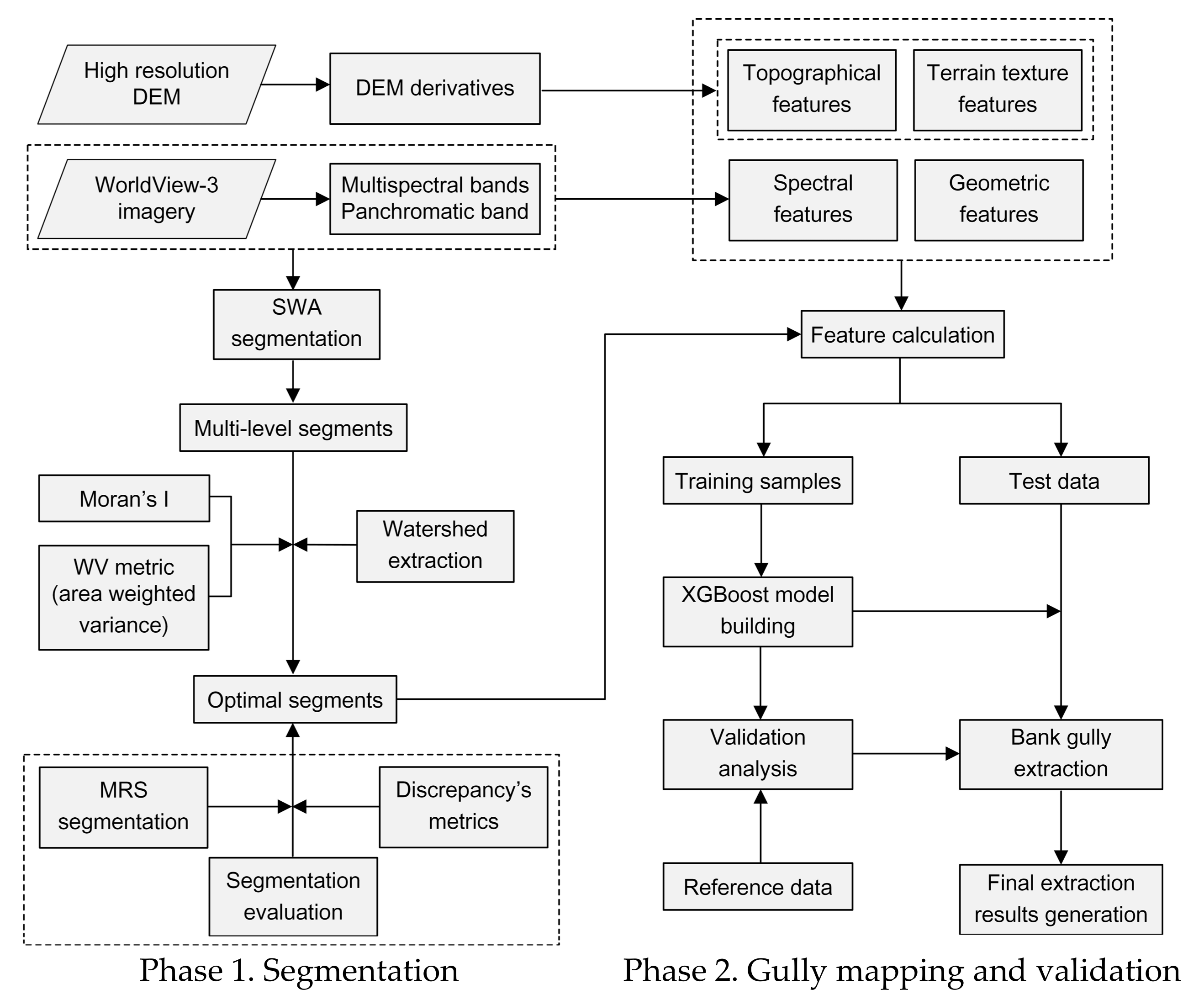
The study site is located in Ansai County, which is in the central part of the Loess Plateau, and belongs to the typical hilly–gully region (Figure 1a). The study area is part of the Zhifanggou catchment and covers an area of 2.33 km² with varying elevation between 1131 m and 1416 m (Figure 1b). It has a semi-arid climate with mean annual precipitation of 528.5 mm and mean temperature of 8.8 °C [9,40,41]. The vegetation coverage has been extremely recovered due to the implementation of the Grain for Green Project since 1999 [7,9,10]. The dominantly tree species in the study area include Robinia pseudoacacia, Caragana intermedia, Hippophae rhamnoides, Sophora viciifolia, Artemisia gmelinii, Artemisia giraldii, Lespedeza davurica and Bothriochloa ischaemun [9,41]. This area has suffered serious soil erosion, which has generated many intensely developed bank gullies in the total area [9], which can be seen in Figure 1c.

In this study, a high-resolution DEM and imagery were used to extract the bank gullies. The DEM, with a 1-m resolution, was generated by using unmanned aerial vehicles (UAVs) and digital aerial photogrammetry [16]. In this study, an MD4-1000 microdrone was applied, which can fly for approximately 45 min at 15 m/s with a recommended payload of 0.80 kg. This microdrone, mounted with a Sony ILCE-7R digital camera system equipped with a 50 mm zoom lens, was able to take pictures of 7360 × 4912 pixels. For the DEM acquisition, two main procedures including outdoor surveying and indoor image processing were carried out.

For the outdoor survey, two steps were needed, namely image acquisition and a ground control survey. (1) Image acquisition: The flight plan was firstly designed by using Waypoint navigation software. Then the images were captured during one flight with an average 60% and 70% overlap in flight strip and flight direction, respectively. The total flight time was 25 min and the flight height was nearly 90 m above ground level. (2) Ground control survey: In this study, two kinds of ground control points (GCPs) were collected, which were 3 base control points (BCPs) and 53 photo control points (PCPs), to maintain the horizontal and vertical accuracies. Each BCP was measured for about 1.5 h by using the Topcon HIPER II G in static mode to build the GPS network for the entire study area. PCP collection was conducted based on Trimble real-time kinematic (RTK) GPS. For the indoor image processing, aerial triangulation was firstly executed for collecting the true positions and orientations of the images. This process was performed by using Trimble’s Info 6.0. After that, the DEM was generated based on MapMatrix 4.0. Then, the DEM at 1 m resolution was finally generated by eliminating buildings and vegetation. Further details of the data acquisition process are described in Liu et al. [16]. To examine the accuracy of the DEM, 37 independent check points (ICPs) were acquired and measured during the outdoor survey. The RMSE value was used to evaluate the vertical and horizontal accuracy. The vertical and horizontal RMSEs in the study area were 0.339 m and 0.187 m, respectively.

Alongside the high-resolution DEM, WorldView-3 Imagery was employed in this research. This imagery contained three visible bands and one near-infrared band with a 1.24 m resolution, and one panchromatic band at a spatial resolution of 0.31 m [17]. An extensive field investigation was accomplished in March 2016 to understand the morphological and distribution pattern of the bank gullies. Then, 110 reference polygons (Figure 2) were manually constructed based on the knowledge from the field investigation, WorldView-3 Imagery and expert knowledge. The reference data set was used for the accuracy assessment, for evaluating both the segmentation accuracy and bank gully extraction accuracy.

2.2. Methods

The proposed bank gully extraction method contained two phases: 1. Segmentation, and 2. Gully mapping and validation. Each processing phase had three steps. For the segmentation phase, the first step was multi-level segment generation. In this step, multispectral bands (three visible bands and one near-infrared band) and panchromatic band were chosen as the input data set. Then, the SWA method was employed to obtain multi-level segments from different segmentation levels. The next step was to optimize the segmentation. The watershed-based segmentation level optimization strategy was utilized by considering both between-segment heterogeneity and within-segment homogeneity, using Moran’s I and WV (area weighted variance) metrics. After that, in the third step of this phase, the segmentation quality was evaluated by using the discrepancy method, and the ANI (area-number index) metric was then proposed by considering both geometric and arithmetic discrepancies. After obtaining the optimal segments, the second phase was initiated, focused on gully extraction and validation. In the first step of this phase, the features, including the spectrum, topography, terrain texture and geometry, were calculated for each segment. The training samples and test data sets were generated in accordance with the watershed boundary. Then, the XGBoost model was trained in the next step. Finally, the bank gully was extracted in the last step.

An overview of the proposed framework is shown in Figure 3.

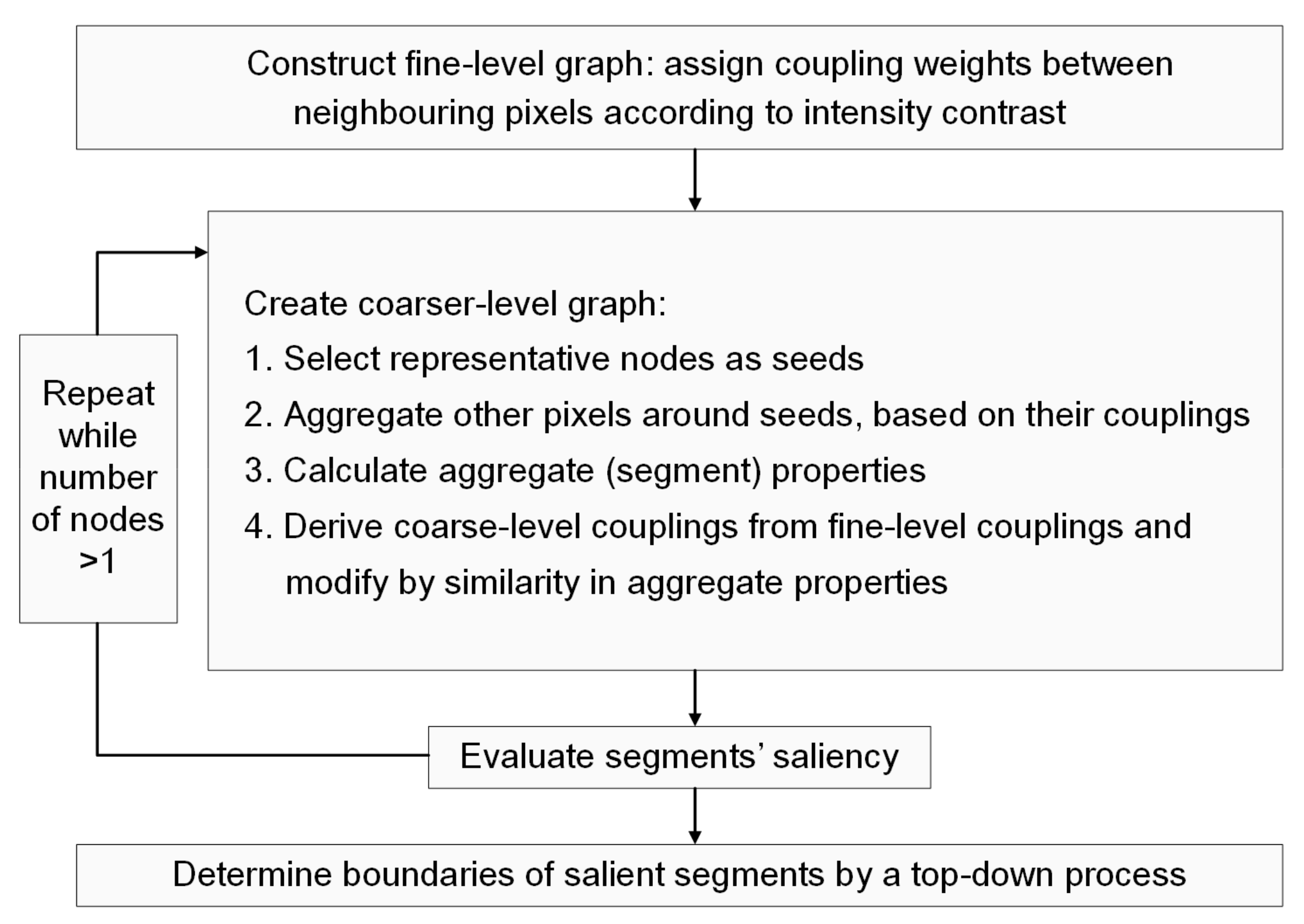
2.2.1. Generating Multi-Level Segments by SWA

The SWA method was first proposed by Sharon et al. [28,29,30] for segmenting natural images hierarchically and efficiently. As shown in Figure 4, it contains four main steps: (1) Fine-level graph construction: In this step, each pixel/segment is treated as a node in a graph, connected with its neighbors in terms of their similarities. (2) Coarser-level graph creation: The coarsening step recursively aggregates to reduce the number of nodes from the finer-level to the coarser-level until only one node is left on the graph, thus generating a pyramid of graphs with larger aggregates of pixels/segments in the coarser levels. After each coarsening process, each new aggregate is formed by multiscale measurements, including the intensities and statistics of textures. All of these measurements are calculated recursively and subsequently used to affect the coupling between neighboring aggregates. (3) Saliency of segments evaluation: The saliency here is defined as the ratio between the within- and between-segment similarities. This ratio is used to find an appropriate segmentation in each level. (4) Determining boundaries of salient segments by a top-down process.

The SWA method is made highly efficient by introducing algebraic multigrid solvers (AMSs) that can reduce the normalized-cut minimization problem in a non-iterative manner [31,32]. The computational complexity of the SWA algorithm is only logarithmic with the number of pixels in the image on a parallel computer.

The consideration of the topographic information has a limited contribution for improving segmentation accuracy, based on our previous knowledge [17]. Therefore, a panchromatic band image combined with another three visible bands and one near-infrared band were selected in this study to feed into SWA for obtaining the multi-level segmentation results.

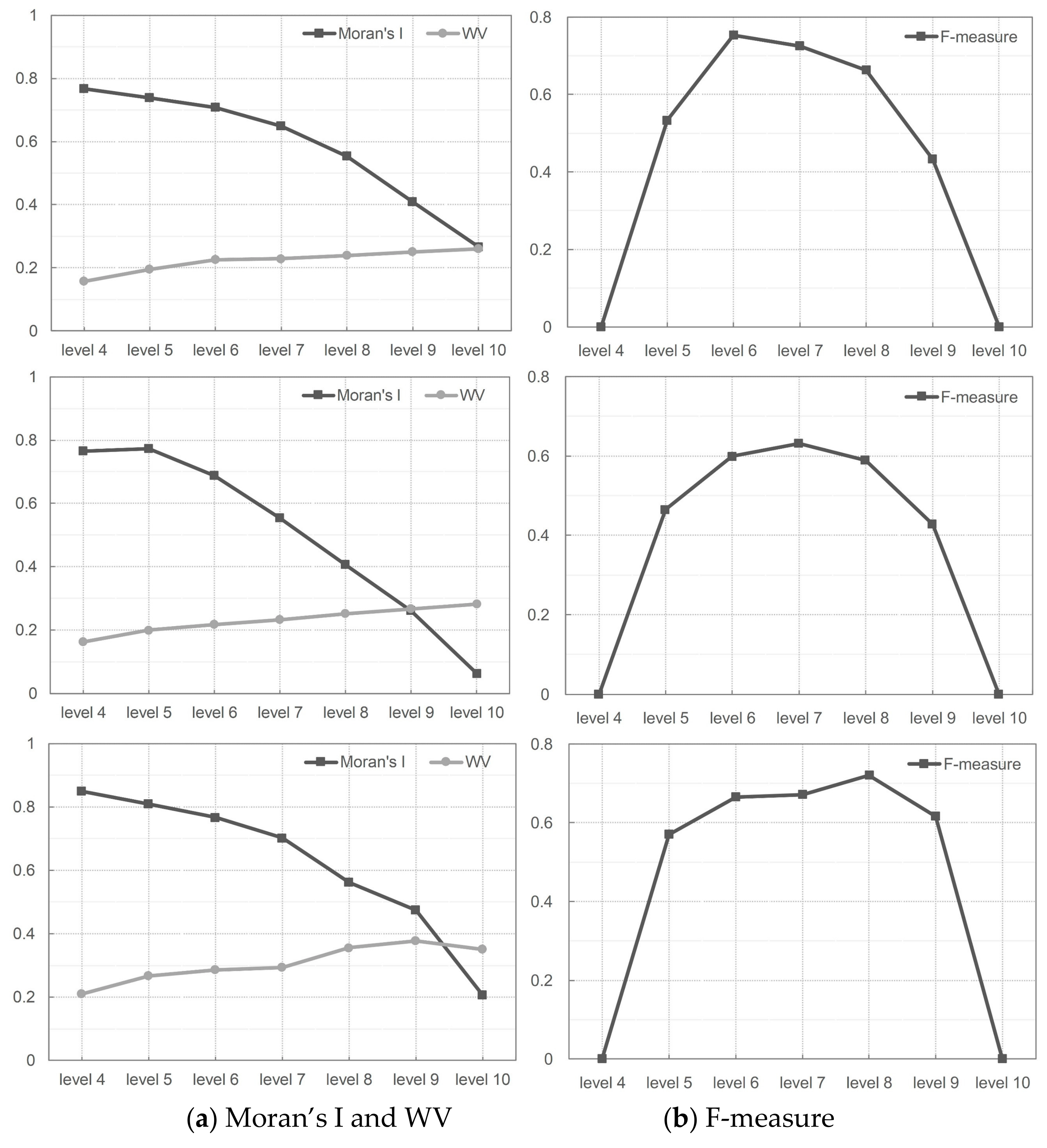
2.2.2. Segmentation Optimization and Evaluation

In this paper, the segmentation optimization strategy first regarded the watershed as the basic processing unit. After that, numbers of sub-watersheds were extracted by following steps. (1) Filled sinks: Sinks were filled based on the DEM [41]. (2) Stream network extraction: Grid-based networks were delineated on the basis of the flow direction calculated by using the D8 algorithm [42] and flow accumulation [41]. (3) Watershed extraction: Based on the flow direction matrix and stream network [43], watersheds were finally extracted with a 0.16 km² threshold. This threshold was automatically determined by following the method of Wu et al. [44]. These processing procedures were fully implemented in the ArcHydro model so that the sub-watersheds could be easily extracted automatically. Finally, 18 sub-watersheds were extracted. Four of them were employed as the training area, and the remaining fourteen sub-watersheds were used for validation. Each sub-watershed had its own segmentation level.

Johnson and Xie [31] pointed out that the issue of whether segments are homogenous and significantly different from neighboring regions should be taken into consideration in order to achieve a good segmentation. To meet these requirements, segmentation level selection should consider both between-segment heterogeneity and within-segment homogeneity [32,45]. In this study, these criteria were measured by employing the commonly used Global Moran’s I (MI) and area-weighted variance (WV) [45,46]. Lower WV values indicate segmentation levels that have a higher within-segment homogeneity, while lower MI values reflect a lower similarity between neighboring segments’ spectral values, which is desirable for a segmentation level [46,47]. The calculations for MI and WV follow the previous paper by Johnson et al. [46].

As mentioned previously, when the MI and WV values of one segmentation are simultaneously higher or lower than those of another, it is easy to determine which is the better segmentation. However, if one segmentation has a higher MI but lower WV, it is difficult to select a better segmentation. Therefore, to find a final optimized segmentation level, the MI and WV values need to be combined into one measurement. The F-measure was suggested to combine the MI and WV in this paper, as Zhang et al. [48] pointed out that the F-measure has less sensitivity to excessive over- and under-segmentation than other commonly used combination methods. Before combining the MI and WV, we first need to normalize them into a similar range from 0 to 1. Then, the F-measure is defined by:

$$F=\frac{M{I}_{norm}·W{V}_{norm}}{a·M{I}_{norm+\left(1-a\right)·WVnorm}}$$

(1)

where a is the relative weights that assign different significance levels to MI_norm and WV_norm. Here, a weight factor of 0.5 was used, indicating equal weighting of MI_norm and WV_norm. MI_norm and WV_norm refer to the normalized MI and WV within a range from 0 to 1. After that, the F-measure can be calculated ranging from 0 to 1, with higher values indicating higher segmentation quality. Then, the optimized segmentation level of each sub-watershed can be determined by the F-measure.

For fully evaluating the segmentation quality, the developed strategy was compared with a state of the art method—multi-resolution segmentation (MRS)—which has been fully implemented in eCognition software and widely used for image segmentation by combining qualitative and quantitative methods. Firstly, visual assessment was employed for qualitative evaluation. After that, the discrepancy-based method was used for the quantitative evaluation of the segmentation results. Here, the discrepancy was categorized into the geometric discrepancy and the arithmetic discrepancy [49]. Specifically, the geometric discrepancy means the spatial overlapping degree between a reference polygon and a corresponding segment [32,49,50]. The arithmetic discrepancy refers to the difference between the number of reference polygons and that of the corresponding segments [49].

Three basic and commonly used geometric discrepancy measures, OS (over-segmentation), US (under-segmentation), and ED (Euclidean distance) [50], and an arithmetic discrepancy metric NSR (Number-of-Segments Ratio) [48], were employed. These indices can be expressed as:

$$OS=1-\frac{{\displaystyle \sum \left|r_i\cap s_j\right|}}{{\displaystyle \sum \left|r_i\right|}},$$

(2)

$$US=1-\frac{{\displaystyle \sum \left|r_i\cap s_j\right|}}{{\displaystyle \sum \left|s_j\right|}},$$

(3)

$$ED=\sqrt{\frac{O{S}^2+U{S}^2}{2}}$$

(4)

$$NSR=\frac{\left|m-v\right|}{m}$$

(5)

where r_i refers to the reference polygons, i = 1, 2, …, m, and s_j is the corresponding segments, j = 1, 2, …, v. $\left|r_i\cap s_j\right|$ denote their spatial overlapped area. m and v denote the number of reference polygons and corresponding segments, respectively. OS and US aim to measure the over-segmentation and under-segmentation degrees. ED is a composite metric considering both OS and US. All of these three indices are ideally near zero and within the range from 0 to 1. NSR is an efficient index designed by Liu et al. [49]. It is defined as the ratio between the difference in the number of reference polygons and corresponding segments and the total number of the reference polygons. A large value of NSR represents a significant over-segmentation situation. A small value of NSR indicates a closer relationship between the reference polygons and corresponding segments.

Considering that the distribution pattern of bank gullies is usually discrete, and their area is always small, as mentioned before, an optimum segmentation should achieve a desirable geometric and arithmetic match simultaneously [49,50]. For this purpose, a new composite index was put forward: the Area-Number Index (ANI), which considers two kinds of discrepancies at one time. The ANI has two parts: the Area Ratio (AR) and the Number Ratio (NR), which can be defined as:

$$NR=\frac{\left|m-v\right|}{\left|m+v\right|}$$

(6)

$$AR=1-\frac{{\displaystyle \sum \left|r_i\cap s_j\right|}}{{\displaystyle \sum \left|r_i\cup s_j\right|}},$$

(7)

where m, v, r_i, and s_j have been defined previously. $\left|r_i\cup s_j\right|$ represents the unionized area of reference polygons and corresponding segments. Both NR and AR range from 0 to 1. A smaller value indicates a better segmentation. Then, the ANI can finally be generated by combining the AR and NR using the previously mentioned F-measure:

$$ANI=\frac{NR·AR}{a·NR+\left(1-a\right)·AR}$$

(8)

Here, the weight a is also assigned a value of 0.5. The values of ANI range from 0 to 1. A small value of ANI means that the geometric discrepancies of the reference polygons and corresponding segments are small, and the relationship between them is nearly one-to-one at the same time. We then used the OS, US, ED, NSR and ANI measures to further compare the segmentation method with MRS.

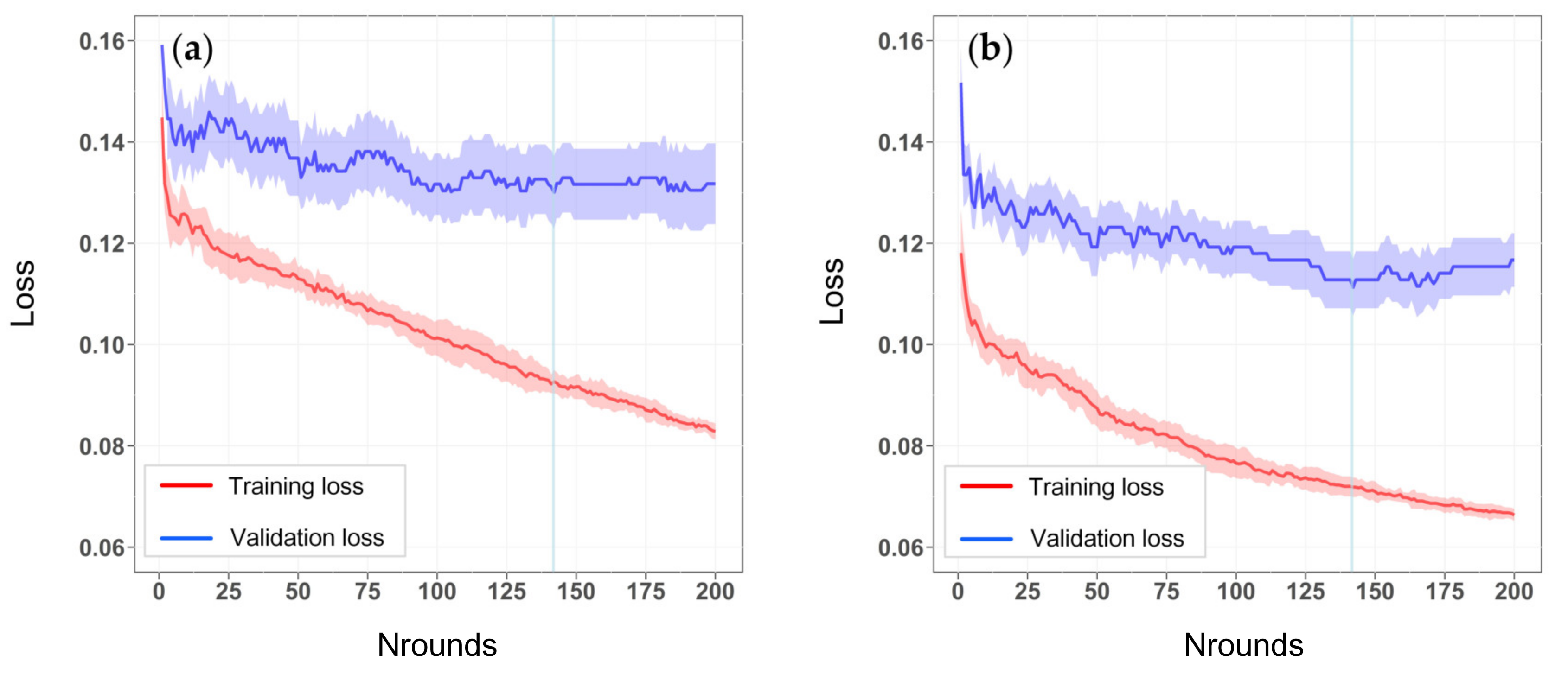
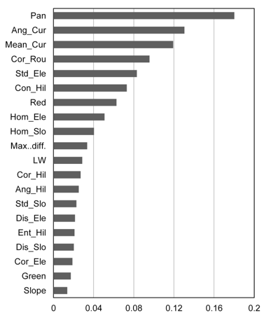
2.2.3. Bank Gully Extraction Using XGBoost

In this study, we used the “XGBoost” package [51,52] implemented in R software to build the model. There are some significant parameters that affect the model’s performance: (1) the number of trees (nrounds) to grow; (2) the learning rate (eta); (3) the parameter that controls the regularization (gamma); (4) the depth of the trees (max_depth), which controls the complexity of the model; (5) the minimum sum of the instance weight (min_child_weight), which determines the stop point of the tree splitting; (6) the number of samples supplied to a tree (subsample); and (7) the number of features supplied to a tree (column_sample). Considering that some of these metrics impact the ability of the model to reduce the overfitting, a fine-tuning process needs to be employed. The 10-fold cross-validation (CV) method was selected to tune the XGBoost model based on the training data set.

For training the model, 55 features were adopted, including spectral, topographical, textural, and geometric characteristics for bank gully extraction. An overview of the features is presented in

Table 1. Overview of the features used for bank gully extraction.

Feature Type	Feature Name	Acronym
Spectral information	Mean band value	Red; Green; Blue; Pan
	Mean brightness	B
	Maximum difference index	MaxDiff
Terrain texture information	Gray Level Co-occurrence Matrix (GLCM) homogeneity	Hom_Ele; Hom_Cur; Hom_Rou; Hom_Slo; Hom_Hil
	GLCM contrast	Con_Ele; Con_Cur; Con_Rou; Con_Slo; Con_Hil
	GLCM dissimilarity	Dis_Ele; Dis_Cur; Dis_Rou; Dis_Slo; Dis_Hil
	GLCM entropy	Ent_Ele; Ent_Cur; Ent_Rou; Ent_Slo; Ent_Hil
	GLCM angular second moment	Ang_Ele; Ang_Cur; Ang_Rou; Ang _Slo; Ang _Hil
	GLCM mean	Mean_Ele; Mean_Cur; Mean_Rou; Mean_Slo; Mean_Hil
	GLCM standard deviation	Std_Ele; Std_Cur; Std_Rou; Std_Slo; Std_Hil
	GLCM correlation	Cor_Ele; Cor_Cur; Cor_Rou; Cor_Slo; Cor_Hil
Topographic information	Mean Elevation	Elevation
	Mean Curvature	Curvature
	Mean Roughness	Roughness
	Mean Slope	Slope
	Mean Shaded relief	Hillshade
Geometric information	Shape index	SI
	Length-width	LW
	Roundness	Roundness
	Area	Area

.

Spectral and geometric features are widely used in object-based image analysis. Additionally, topography is a key factor for a gully’s development [53,54]. In this paper, five basic topographic factors, namely elevation, curvature, slope, roughness and shaded relief, were chosen. Then, the mean values of these factors were calculated for each segment. Moreover, terrain texture features were also used, since they can improve the accuracy of gully feature extraction [19]. Eight terrain texture measures, derived from the Gray Level Co-occurrence Matrix (GLCM) proposed by Haralick [55], were calculated based on five topographic features.

Another issue that affects the XGBoost model is feature selection. In the XGBoost model, the feature selection is determined by feature importance based on Mean Decrease on Gini (MDG). MDG measures the improvement in the purity of nodes by each variable. A feature which has a higher MDG value will have a higher feature importance.

After the bank gullies were predicted by the XGBoost model, the validation of the predicted results was based on the reference data. Considering that the bank gullies only cover an extremely small area, the aim of this case was focused on determining whether the gullies could be extracted at all. Therefore, the accuracy assessment of the bank gully extraction was based on the gully number. If the overlapping area between an extracted gully and the reference data was over 50%, this segment could be treated as a correct one. Then, four values, namely the Ture positive (TP), False positive (FP) and False negative (FN) were determined for calculating three commonly used accuracy assessment metrics, such as the Precision (Pr), Recall (Re), F1-score (F1). The TP is the number of segments that are correctly detected as bank gullies. FPs correspond to the number of segments that are identified as gullies but are not included in the reference data sets. FNs represent the number of gullies in reference polygons that are not detected by the utilized method. Therefore, Pr was used to measure how many of the segments extracted by the applied method were actual bank gullies. Re was used to determine how many of the reference polygons could be detected as bank gullies. The F1 is the harmonic average of Pr and Re, which can reflect the balance between these two accuracy parameters and can be used to assess the overall accuracy [56].

3. Results and Analysis

In this study, bank gullies were extracted after carrying out two experiments. Firstly, an optimized segmentation result was selected by using proposed watershed-based optimization strategy from 20 levels of segmentation generated by SWA. After that, fine-tuned XGBoost was adopted and bank gullies were finally detected. The experiment results of segmentation and gully mapping were discussed separately for the sake of clarity.

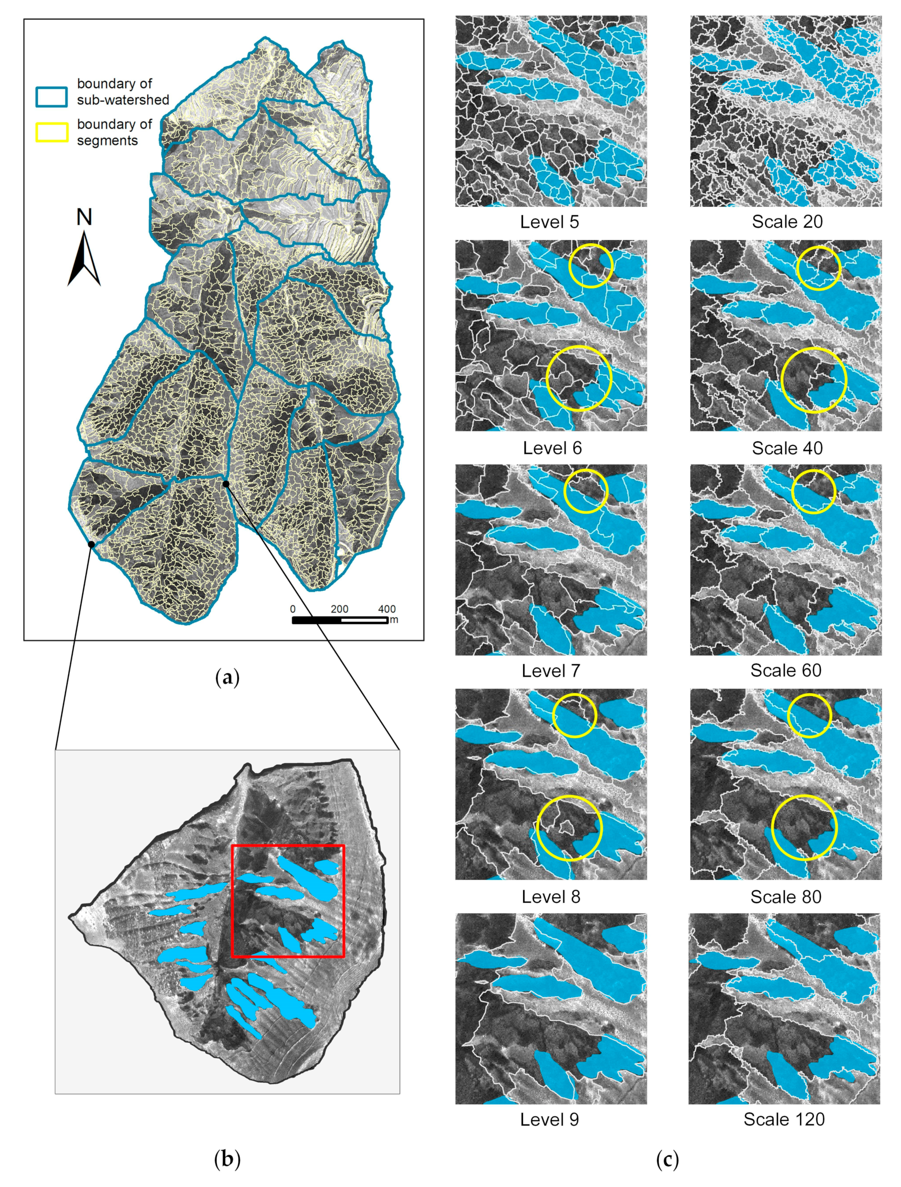
3.1. Segmentation Results

SWA produced 20 levels of segmentation results ranging from over-segmentation to under-segmentation at one time. As the segments of levels 1–4 and levels 10–20 were extremely over-segmented and under-segmented, the optimum segmentation level was considered to lie within levels 5–9. Then, the MI and WV measures and the combined metric F-measure were calculated based on multi-level results for each sub-watershed, and they are plotted as curves in Figure 5. To better display the variation trends of MI, WV, and F-measure, the results for levels 4 and 10 were also plotted. Due to the paper length limitation, only three sub-watershed calculation results are shown in Figure 5.

As shown in Figure 5a from level 4 to level 10, the MI value increases, and the WV value decreases slightly for the sub-watersheds. This means that when only using MV and WI we cannot directly determine the optimal segmentation level due to the opposite variation trend. The combination metric, F-measure, was then calculated to solve this difficulty, and is plotted in Figure 5b. As mentioned in Section 2.2.2, a larger value for the F-measure indicates a higher quality of the segmentation. Therefore, the optimum segmentation levels for these sub-watersheds was achieved based on the results displayed in Figure 5, which are level 6, level 7 and level 8, respectively. Therefore, the optimum segmentation level of the rest of the 15 sub-watersheds was determined using the same method, and the final results are illustrated in

Table 2. The optimized segmentation level for each sub-watershed.

Optimized Level	Sub-Watersheds
Level 6	Sub-watershed 1, 2, 3, 6, 8, 10, 11, 12, 17
Level 7	Sub-watershed 4, 5, 9, 14, 15, 16
Level 8	Sub-watershed 7, 13, 18

.

As mentioned before, the segmentation performance was qualitatively and quantitatively compared with MRS. Firstly, five segmentations were generated by MRS with the scales of 20, 40, 60, 80 and 120. The number of segments produced by these five scales was relatively close to that of the SWA method from level 5 to level 9. Then, the segments produced by each level of MRS were visually compared with the results generated by each level of SWA, as illustrated in Figure 6. Quantitative evaluation results of the performances of the two segmentation methods, based on the five metrics mentioned in Section 2.2.3, are also presented in

Table 3. Segmentation quality metrics of quantitative comparisons between SWA and MRS results.

Method	Num. of Segments	Level/ Scale	OS	US	ED	NSR	AR	NR	ANI
SWA	3445	Opt	0.078	0.106	0.093	5.576	0.078	0.627	0.138
1 SWA	12,000	Level 5	0.079	0.066	0.073	24.981	0.079	0.910	0.145
MRS	13,712	20	0.056	0.058	0.056	31.660	0.077	0.937	0.142
2 SWA	4770	Level 6	0.078	0.083	0.081	9.830	0.079	0.796	0.143
MRS	4895	40	0.103	0.130	0.118	10.962	0.103	0.818	0.184
3 SWA	2027	Level 7	0.080	0.246	0.183	3.802	0.081	0.525	0.140
MRS	1807	60	0.095	0.222	0.171	4.057	0.107	0.507	0.176
4 SWA	966	Level 8	0.100	0.352	0.259	1.726	0.098	0.462	0.161
MRS	1059	80	0.117	0.562	0.406	2.340	0.115	0.539	0.190
5 SWA	601	Level 9	0.129	0.639	0.461	1.019	0.120	0.337	0.177
MRS	506	120	0.198	0.798	0.581	0.943	0.181	0.321	0.231

The number in the left column of each row represents the comparison group number. Num. of segments: Number of segments; Opt: Optimized segmentation level of SWA

.

To better illustrate the visual assessment evaluation results, sub-watershed 1 and its subset, which is highlighted by a red rectangle in Figure 6b, were chosen for detailed comparison of MRS and the proposed method. As shown in Figure 6, the segmentation results of each level of SWA and each scale of MRS were grouped together. For level 5 and scale 20, both methods achieved reasonable segment boundaries. However, the segmentations were extremely over-segmented, and it was hard to distinguish directly which one was the better result. For level 9 and scale 120, both segmentations were obviously under-segmented. Based on

Table 4. Optimized parameters of the Extreme Gradient Boosting (XGBoost) model.

Parameters	Default Values	Optimized Values
nrounds	600	141
eta	0.3	0.1
gamma	0	0
max_depth	6	6
min_child_weight	1	2
subsample	1	0.5
column_sample	1	0.5

, level 6 is the optimum segmentation level for sub-watershed 1. As shown in Figure 6c, although the segments of level 6 were slightly over-segmented, the boundaries were still more accurate than those of level 7 and level 8. Compared with the segments of MRS at scale 40, SWA generated more precise segments, since MRS at this scale demonstrated under-segmentation in several segments, especially in areas highlighted by yellow circles. The same phenomenon also appeared in level 7 and level 8 when compared with scale 60 and scale 80.

In addition, the quantitative comparison results are demonstrated in Table 3. As shown in the table, with increasing segmentation level (SWA) or scale (MRS), the ED values of the two segmentation methods increased, which indicated that the segments generated by low levels or scales were more consistent with the reference polygons. Meanwhile, the NSR values decreased from a low segmentation level or scale to a high level or scale. They achieved their minimum at level 9 and scale 120 for SWA and MRS, respectively, implying that a higher segmentation level or scale could better achieve a one-to-one relationship between a reference polygon and its corresponding segment. Therefore, the ANI metric, which considered both geometric and arithmetic discrepancies, was employed to further evaluate the segmentation performance. As shown in Table 3, the ANI values in the four comparison groups (Groups 2, 3, 4 and 5) of SWA were lower than MRS. This indicates that, in most cases, SWA outperformed MRS, which was consistent with the conclusion of the qualitative comparison. The minimum ANI for MRS was 0.142 at scale 20, and was 0.145 at level 6 for SWA. However, the value was still higher than that of SWA with the optimum segmentation level. It obtained the lowest ANI of 0.138, implying that a balanced segmentation result can be achieved at the optimized segmentation level by SWA.

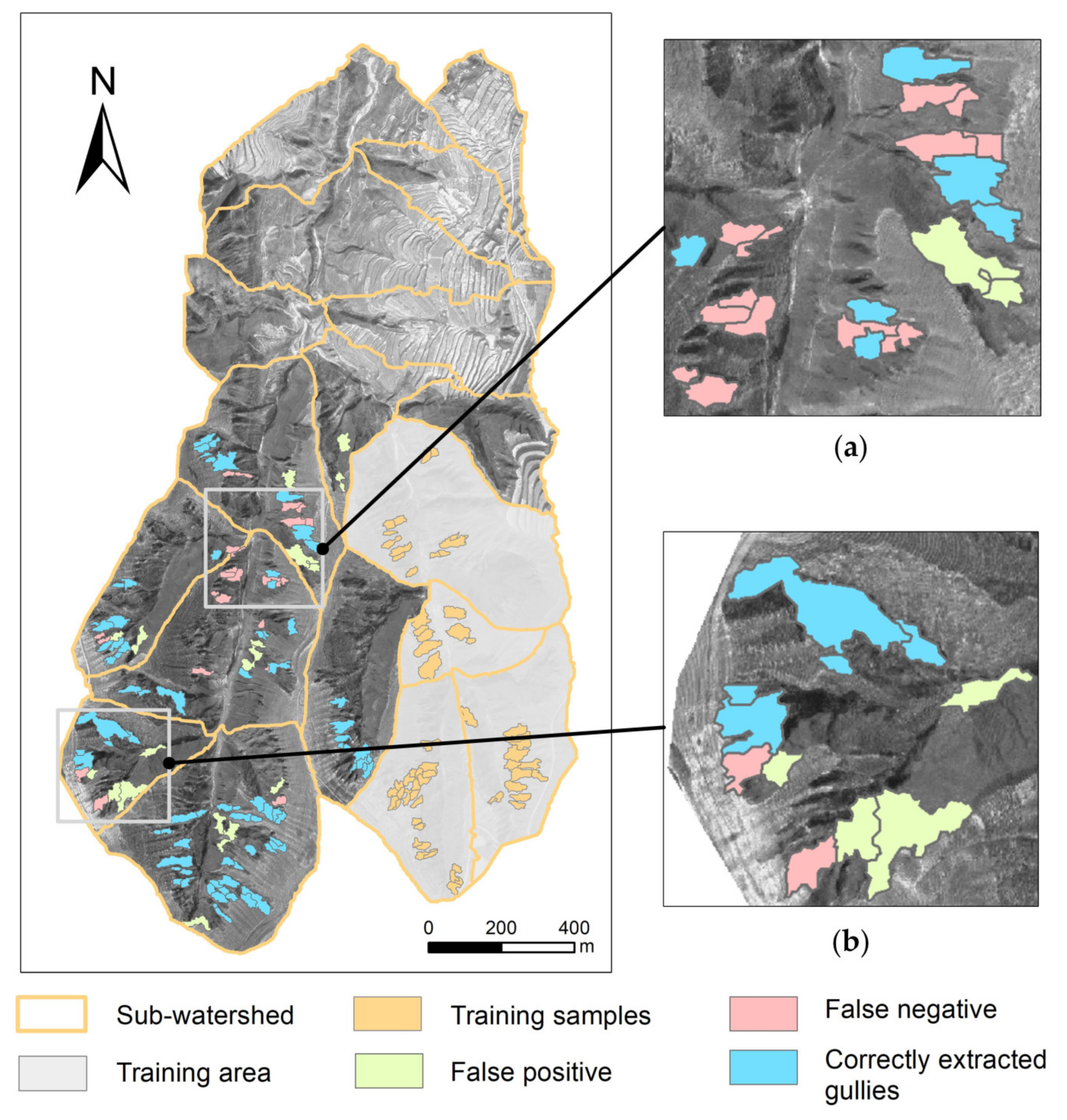
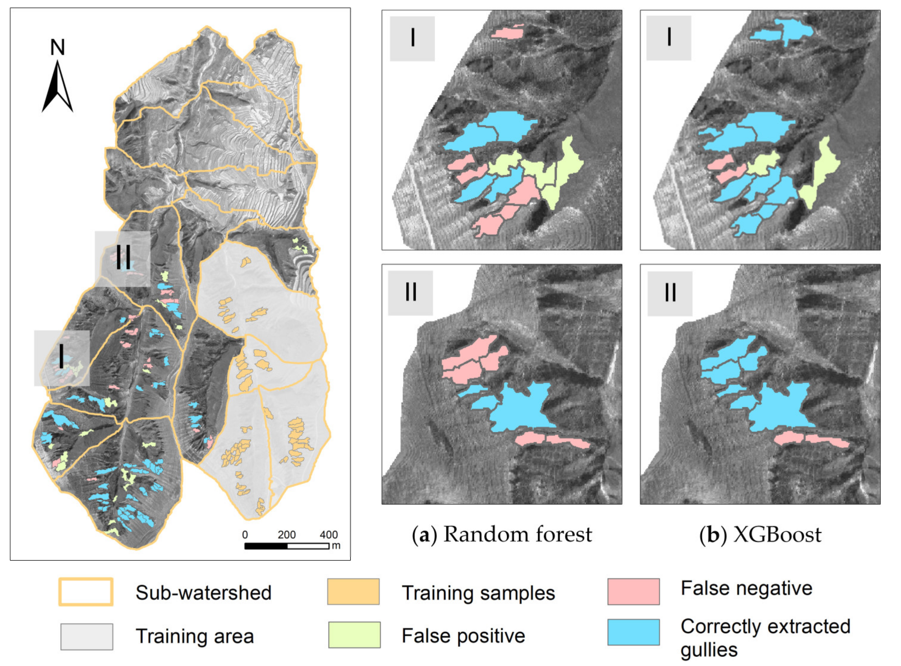
3.2. Bank Gully Extraction Results

According to the segmentation results, four sub-watersheds were selected as the training area to train the XGBoost model. The training area contains 771 segments. These segments have 62 positive samples and 709 negative samples. They were used to train the XGBoost model. The remaining 15 sub-watersheds, which have 2674 segments, were used to validate the model. Then, the fine-tuning process was employed by using 10-fold CV, as mentioned in Section 2.2.3, based on training data sets. We first set the nrounds as 600 and other metrics as default (Table 4). After that, the early stopping strategy was adopted during the training stage to determine the optimized nrounds. Then, the learning curves were recorded, and they are displayed in Figure 7a. The validation error in Figure 7a reached the lowest position at 141 nrounds and then became nearly stabilized, however, the training loss kept dropping down. This circumstance evidenced that model started to “memorize” the training data and refused to “learn” how to generalize the feature of bank gullies at that time, which meant that the model tended to be overfitting after 141 nrounds [57]. Therefore, the optimized nrounds was set at 141. Hereafter, the grid search method based on 10-fold CV was used to fine-tune other parameters. As can be seen from Figure 7b, the validation loss of the model after fine-tuning was lower than it was before. The final optimized parameters are presented in Table 4. The fine-tuned XGBoost model was then introduced to predict the bank gully.

To present the feature importance ranking, we calculated the mean value of the MDG from 15-fold replicate runs, and the top 20 features were selected and presented in Figure 8. The terrain texture features dominated the feature importance ranking, with 14 features selected. This is because the GLCM-based terrain texture can fully consider the spatial relationship among pixels. This capability provides terrain texture a reliable basis for reflecting the assemblages of repeating patterns of landform elements [57]. GLCM-based terrain texture can be treated as a kind of second-order geomorphometric parameter. The use of these second-order parameters can enhance the ability of traditional topographic factors to distinguish different landform types. Therefore, terrain textures can better identify distinctions among different landforms at a certain scale than traditional topographic features [58]. Excepting terrain texture features, there was only one geometric and one topographical feature appearing in the ranking list, implying a minimal effect for these two kinds of metrics in improving the accuracy of bank gully extraction. As shown in Figure 8, the Pan feature ranked at the top position. This may be because the panchromatic band has 0.31 m resolution and the features obtained from higher resolution imagery are more important than those from the 1-m resolution DEM.

The XGBoost model for mapping bank gullies was created by employing all the features with 62 gully segments and 644 non-gully segments, and applied on the remainder validation data sets. The result is demonstrated in Figure 9, with 78.57% for the F1, and with 80.21% and 77.00% for the Pr and Re, respectively (

Table 5. Accuracy assessment for the bank gully extraction result.

		Prediction		Pr	Re	F1
		Gully	Non-Gully
Reference	Gully	77	23	80.21%	77.00%	78.57%
	Non-gully	19	2555

). As for the bank gully extraction result, the error was caused by several factors. As shown in Figure 10a, the topography in this intersection area of three sub-watersheds was complex, blurring the boundaries of the bank gullies so that some gullies were not detected in this area. Moreover, there were also some commission errors, especially in the headwater area, which can be seen in Figure 10. These incorrectly extracted segments belong to ephemeral river channels.

4. Discussion

As the experiments in this study demonstrated, the proposed method had already successfully extracted bank gullies. Although the accuracy of the mapping result is acceptable, a comparative analysis still needs to verify the efficiency of the proposed method. In addition, its applications and limitations also need to be discussed.

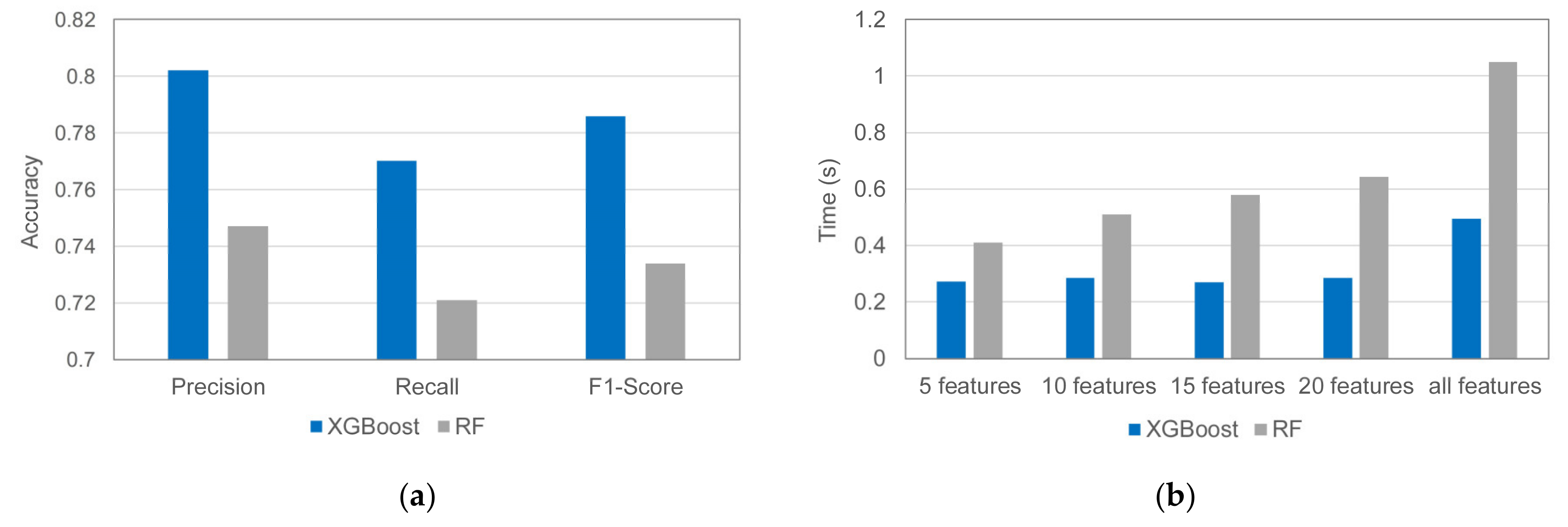
4.1. Comparison With Another Method

The effectiveness of the proposed method was further revealed by comparing it with RF, which is the most popular ensemble classifier for the classification of remote sensing images [38,54]. This supervised method can create a forest of CART-like decision trees based on bootstrap sampling and randomized node optimization. The bootstrap is a kind of random sampling replacement method. Currently, RF is widely used in the earth science community due to its high classification accuracy and processing speed [38]. Two parameters need to be determined to generate the model: (1) the number of trees needing to be grown (nTree), and (2) the number of features that are selected randomly at each node (mTry). We used the RF package, which was implemented in R language to build the extraction model. The nTree and mTry were set to 500 and the square root of the total features number, respectively. The features and training area were kept the same as in XGBoost. The class imbalance effect was also considered, and the analysis results also suggested using all the 55 features to build the model.

The predicted results are illustrated in Figure 11. Then, two close-up subsets were selected to further demonstrate the differences in the extraction results between RF and XGBoost (Figure 11a,b). After that, the comparison of the precision, recall and F1-score and the processing time were investigated to further assess the effectiveness of the two methods (Figure 9). As shown in the two subsets in Figure 11, some gullies omitted by RF were extracted by XGBoost, especially in the headwater area. Moreover, XGBoost can achieve a relatively higher recall than RF (4.9%), which implies that XGBoost can alleviate omission errors more effectively than RF. However, some commission errors are also detected by both methods in the ephemeral channel (Figure 11, subset I). As shown in Figure 9b, the processing time of XGBoost with 500 nrounds is nearly twice as short as RF with 500 nTree in general. Further, the advantage of XGBoost in operating time is gradually expanded when the number of features increases (Figure 9b), indicating that XGBoost is more suitable for processing large data volumes than RF. The reason for which XGBoost outperforms RF is mainly attributed to the model structures. Different from RF, XGBoost is a kind of boosting model. It sequentially trains individual decision trees (DTs), and each DT is an improved version of the previous one, which leads to a smaller error rate [38]. Besides, XGBoost uses a regularization term to constrain the model, which is beneficial to controlling the model complexity and can reduce overfitting [39,59].

In previous studies, some work used drainage network information to extract bank gullies [60]. Although this method can effectively extract bank gullies and detect their real positions, the mapping process is uncertain and not universal. Moreover, this method can only reflect structural features of bank gullies. Therefore, the proposed object-based approach is superior than the drainage network-based method, since objects can essentially bridge the gap between geographic entities and image elements [32], allowing inherent characteristics, including spectral, textural, and shape properties, to be fully exploited. Recently, deep learning-based studies have become popular for remote sensing-based landform mapping research [56,61]. Zhang et al. [62] used Mask R-CNN to automatically characterize Arctic ice-wedge polygons and achieved as high as 90% accuracy. Since ice-wedge polygons have similar characteristics with bank gullies, which occupy a very small area and are distributed discretely, the Mask R-CNN method has great potential for mapping bank gullies. However, directly transferring this method to extract bank gullies is not easy, because training a deep learning model usually requires a large number of samples and may also require a data augmentation technique. Therefore, the issue of how to collect enough training data sets and design an appropriate data augmentation strategy needs to be fully exploited.

4.2. Applications and Limitations of the Proposed Method

The proposed method presented the potentials of UAV photogrammetry for bank gully extraction. As the availability of high-resolution DEMs increases, the question then is whether the bank gully extraction requires a sub-meter DEM and for what purpose will it be needed. Tarolli [63] pointed out that there is no perfect resolution, and the selection of the appropriate resolution can be determined based on the size of an object. Considering the average width of a bank gully was more than 1 m, adopting a meter-level DEM was suitable for bank gully mapping in this study. Although bank gullies are one of the most significant sources of sediment yield, other gully types are also worth detecting. High-resolution DEMs generated by UAVs make gully mapping at different types possible. Existing studies have also presented the potentials of UAV photogrammetry for hillslope and bank gully extraction [16,64]; however, mapping floor gullies is particularly difficult. Floor gullies usually develop in the bottom part of a valley with a very deep situation, which is difficult to reflect using UAV photogrammetry. In this circumstance, floor gully detection still relies on the traditional field survey.

Moreover, the proposed method could be applied in other regions within the hilly Loess Plateau by considering the following. Firstly, although the landform in the Loess Plateau has spatial heterogeneity, the distribution pattern of gullies has a certain regularity. In addition, this study was carried out in an area with complex terrain features that have suffered severe soil erosion. The successful application of the proposed method in this area proves its transferability to other hilly Loess Plateau regions. The basic idea of the strategy employed by this study is universality, including segmentation, the generation of features, and classification, such that it can potentially be extrapolated outside the Loess Plateau. However, challenges still remain. The significant differences in gully erosion conditions may lead to hugely different gully sizes, shapes, and densities [10]. Therefore, field investigations may need to be executed before employing the proposed method. Further, the parameters of this study should be adapted to the specific area.

5. Conclusions

Previous OBIA methods of bank gully extraction relied on setting parameters to generate multi-scale segmentations. Further, the segmentation optimization procedure usually neglected to consider the inherent scales of gullies. To overcome such issues, we developed an integrated OBIA framework for mapping bank gullies, including image segmentation, scale optimization, and segmentation evaluation.

Four improvements were achieved in this study: (1) the segmentation step was combined with SWA and the watershed extraction strategy to produce segmentations at quasi-continuous scales; (2) the segmentation level optimization step treated the watershed as a basic processing unit and considered both between-segment heterogeneity and within-segment homogeneity; (3) we proposed a new discrepancy metric, the ANI value, to evaluate the segmentation results; and (4) we employed the XGBoost method to improve the classification accuracy. Based on the comparative analysis results, the segmentation achieved by the proposed method outperformed the state of the art MRS method. Moreover, the accuracy of the bank gully mapping result was superior to RF, achieving a 5% higher accuracy. These experimental results indicate that the developed approach is effective and could be useful for researchers to monitor gully erosion. In addition, the presented framework may have the ability to be applied in other regions within the Loess Plateau, since the basic idea for the approach is generalizable.

From an application perspective, there are still some shortcomings of the proposed approach that can be improved further: (1) the extraction accuracy could be improved by using a superior algorithm, such as a deep convolutional neural network; and (2) the robustness and universality of the method could be improved by employing an unsupervised segmentation evaluation method in future works.

References

1. Poesen, J.; Nachtergaele, J.; Verstraeten, G.; Valentin, C. Gully erosion and environmental change: Importance and research needs. Catena 2003, 50, 91–133. [Google Scholar] [CrossRef]
2. Upper and Middle Yellow River Bureau. Atlas of Soil and Water Conservation in the Yellow River Basin; Seismological Press: Beijing, China, 2012. [Google Scholar]
3. Wu, H.; Xu, X.; Zheng, F.L.; Chao, Q.; Xu, H. Gully Morphological Characteristics in the Loess Hilly-gully Region Based on 3D Laser Scanning Technique. Earth Surf. Process. Landf. 2017, 43, 1701–1710. [Google Scholar] [CrossRef]
4. Gao, H.D.; Li, Z.B.; Li, P.; Jia, L.L.; Xu, G.C.; Ren, Z.P.; Pang, G.W.; Zhao, B.H. Capacity of soil loss control in the Loess Plateau based on soil erosion control degree. J. Geogr. Sci. 2016, 26, 457–472. [Google Scholar] [CrossRef] [Green Version]
5. Tang, G.A.; Li, F.Y.; Liu, X.J.; Long, Y.; Yang, X. Research on the slope spectrum of the Loess Plateau. Sci. China Ser. E 2008, 51, 175–185. [Google Scholar] [CrossRef]
6. Zheng, F.L.; Xu, X.M.; Qin, C. A review of gully erosion process research. Trans. CSAE 2016, 47, 48–59, (In Chinese with English Abstract). [Google Scholar]
7. Li, Z.; Zhang, Y.; Zhu, Q.; Yang, S.; Li, H.; Ma, H. A gully erosion assessment model for the Chinese Loess Plateau based on changes in gully length and area. Catena 2017, 148, 195–203. [Google Scholar] [CrossRef]
8. Liu, K.; Ding, H.; Tang, G.A.; Song, C.Q.; Jiang, L.; Zhao, B.Y.; Gao, Y.F.; Ma, R.H. Large-scale mapping of gully-affected areas: An approach integrating google earth images and terrain skeleton information. Geomorphology 2018, 314, 13–26. [Google Scholar] [CrossRef]
9. Chen, Y.X.; Jiao, J.Y.; Wei, Y.H.; Zhao, H.K.; Yu, W.J.; Cao, B.T.; Xu, H.Y.; Yan, F.C.; Wu, D.Y.; Li, H. Accuracy Assessment of the Planar Morphology of Valley Bank Gullies Extracted with High Resolution Remote Sensing Imagery on the Loess Plateau, China. Int. J. Env. Res. Pub. Health 2019, 16, 369. [Google Scholar] [CrossRef] [Green Version]
10. Li, Z.; Zhang, Y.; Zhu, Q.; He, Y.; Yao, W. Assessment of bank gully development and vegetation coverage on the Chinese Loess Plateau. Geomorphology 2015, 228, 462–469. [Google Scholar] [CrossRef]
11. Wu, Y.; Cheng, H. Monitoring of gully erosion on the Loess Plateau of China using a global positioning system. Catena 2005, 63, 154–166. [Google Scholar] [CrossRef]
12. Shruthi, R.B.V.; Kerle, N.; Jetten, V. Object-based gully feature extraction using high spatial resolution imagery. Geomorphology 2011, 134, 260–268. [Google Scholar] [CrossRef]
13. Peter, K.D.; d’Oleire-Oltmanns, S.; Ries, J.B.; Marzolff, I.; Hssaine, A.A. Soil erosion in gully catchments affected by land-levelling measures in the Souss Basin, Morocco, analysed by rainfall simulation and UAV remote sensing data. Catena 2014, 113, 24–40. [Google Scholar] [CrossRef]
14. Shruthi, R.B.V.; Kerle, N.; Jetten, V.; Stein, A. Object-based gully system prediction from medium resolution imagery using Random Forests. Geomorphology 2014, 216, 283–294. [Google Scholar] [CrossRef]
15. D’Oleire-Oltmanns, S.; Marzolff, I.; Tiede, D.; Blaschke, T. Detection of gully-affected areas by applying Object-Based Image Analysis (OBIA) in the region of Taroudannt, Morocco. Remote Sens. 2014, 6, 8287–8309. [Google Scholar] [CrossRef] [Green Version]
16. Liu, K.; Ding, H.; Tang, G.A.; Na, J.M.; Huang, X.L.; Xue, Z.G.; Yang, X.; Li, F.Y. Detection of Catchment-Scale Gully-Affected Areas Using Unmanned Aerial Vehicle (UAV) on the Chinese Loess Plateau. ISPRS J. Photogramm. Remote Sens. 2016, 5, 238. [Google Scholar] [CrossRef]
17. Liu, K.; Ding, H.; Tang, G.; Zhu, A.X.; Yang, X.; Jiang, S.; Cao, J. An Object-based Approach for Two-level Gully Feature Mapping Using High-resolution DEM and Imagery: A Case Study on Hilly Loess Plateau Region, China. Chin. Geogr. Sci. 2017, 27, 415–430. [Google Scholar] [CrossRef]
18. Baatz, M.; Schäpe, A. Multiresolution segmentation. In Angewandte Geographische Informationsverarbeitung XII; Herbert Wichmann Verlag: Heidelberg, Germany, 2000; pp. 12–23. [Google Scholar]
19. Drǎguţ, L.; Tiede, D.; Levick, S.R. ESP: A tool to estimate scale parameter for multiresolution image segmentation of remotely sensed data. Int. J. Geogr. Inf. Sci. 2010, 24, 859–871. [Google Scholar] [CrossRef]
20. Du, S.H.; Guo, Z.; Wang, W.Y.; Guo, L.; Nie, J. A comparative study of the segmentation of weighted aggregation and multiresolution segmentation. Gisci. Remote. Sens. 2016, 53, 651–670. [Google Scholar] [CrossRef]
21. Xiong, Z.Q.; Zhang, X.Y.; Wang, X.N.; Yuan, J. Self-adaptive segmentation of satellite images based on a weighted aggregation approach. Gisci. Remote. Sens. 2018, 1–23. [Google Scholar] [CrossRef]
22. Blaschke, T. Object based image analysis for remote sensing. ISPRS J. Photogramm. Remote Sens. 2010, 65, 2–16. [Google Scholar] [CrossRef] [Green Version]
23. Cheng, H.D.; Sun, Y. A hierarchical approach to color image segmentation using homogeneity. IEEE T. Image Process. 2000, 9, 2071–2082. [Google Scholar]
24. Camilus, K.S.; Govindan, V.K. A Review on Graph Based Segmentation. I. J. Image Graph. Signal Process. 2012, 4. [Google Scholar] [CrossRef] [Green Version]
25. Eriksson, A.; Olsson, C.; Kahl, F. Normalized cuts revisited: A reformulation for segmentation with linear grouping constraints. J. Math Imaging Vis. 2011, 39, 45–61. [Google Scholar] [CrossRef] [Green Version]
26. Grady, L. Random walks for image segmentation. IEEE T. Pattern Anal. 2006, 1768–1783. [Google Scholar] [CrossRef] [Green Version]
27. Zeng, Y.; Samaras, D.; Chen, W.; Peng, Q.S. Topology cuts: A novel min-cut/max-flow algorithm for topology preserving segmentation in N–D images. Comput. Vis. Image Und. 2008, 112, 81–90. [Google Scholar] [CrossRef]
28. Sharon, E.; Brandt, A.; Basri, R. Fast multiscale image segmentation. In Proceedings of the IEEE Conference on Computer Vision and Pattern Recognition (CVPR 2000), Hilton Head Island, SC, USA, 13–15 June 2000. [Google Scholar]
29. Sharon, E.; Brandt, A.; Basri, R. Segmentation and boundary detection using multiscale intensity measurements. In Proceedings of the IEEE Conference on Computer Vision and Pattern Recognition (CVPR 2001), Kauai, HI, USA, 8–14 December 2001. [Google Scholar]
30. Sharon, E.; Galun, M.; Sharon, D.; Basri, R.; Brandt, A. Hierarchy and adaptivity in segmenting visual scenes. Nature 2006, 442, 810. [Google Scholar] [CrossRef]
31. Johnson, B.; Xie, Z.X. Unsupervised image segmentation evaluation and refinement using a multi-scale approach. ISPRS J. Photogramm. Remote Sens. 2011, 66, 473–483. [Google Scholar] [CrossRef]
32. Zhang, X.Y.; Du, S.H.; Ming, D.P. Segmentation Scale Selection in geographic object-based image analysis. In High Spatial Resolution Remote Sensing: Data, Analysis, and Applications, 1st ed.; CRC Press: Boca Raton, FL, USA, 2018; pp. 201–228. [Google Scholar]
33. Zhang, X.Y.; Du, S.H. Learning selfhood scales for urban land cover mapping with very-high-resolution satellite images. Remote Sens. Environ. 2016, 178, 1721–1790. [Google Scholar] [CrossRef]
34. Zhang, X.L.; Xiao, P.F.; Feng, X.Z.; Feng, L.; Ye, N. Toward evaluating multiscale segmentations of high spatial resolution remote sensing images. IEEE Trans. Geosci. Remote Sens. 2015, 53, 3694–3706. [Google Scholar] [CrossRef]
35. Xu, L.; Ming, D.P.; Zhou, W.; Bao, H.Q.; Chen, Y.Y.; Ling, X. Farmland Extraction from High Spatial Resolution Remote Sensing Images Based on Stratified Scale Pre-Estimation. Remote Sens. 2019, 11, 108. [Google Scholar] [CrossRef] [Green Version]
36. Chen, Y.Y.; Ming, D.P.; Zhao, L.; Lv, B.R.; Zhou, K.Q.; Qing, Y.Z. Review on high spatial resolution remote sensing image segmentation evaluation. Photogramm. Eng. Remote Sens. 2018, 84, 629–646. [Google Scholar] [CrossRef]
37. Xiong, L.Y.; Zhu, A.X.; Zhang, L.; Guo, A.T. Drainage basin object-based method for regional-scale landform classification: A case study of loess area in China. Phys. Geogr. 2018, 39, 523–541. [Google Scholar] [CrossRef]
38. Jozdani, S.E.; Johnson, B.A.; Chen, D. Comparing Deep Neural Networks, Ensemble Classifiers, and Support Vector Machine Algorithms for Object-Based Urban Land Use/Land Cover Classification. Remote Sens. 2019, 11, 1713. [Google Scholar] [CrossRef] [Green Version]
39. Chen, T.; Guestrin, C. XGBoost: Reliable Large-Scale Tree Boosting System. arXiv 2016, 1–6. [Google Scholar]
40. Zhou, D.; Zhao, S.; Zhu, C. The Grain for Green Project induced land cover change in the Loess Plateau: A case study with Ansai County, Shanxi Province, China. Ecol. Indic. 2012, 23, 88–94. [Google Scholar] [CrossRef]
41. Tarboton, D.G.; Bras, R.L.; Rodriguez-Iturbe, I. On the extraction of channel networks from digital elevation data. Hydro. Process. 1991, 5, 81–100. [Google Scholar] [CrossRef]
42. Jenson, S.K.; Domingue, J.O. Extracting topographic structure from digital elevation data for geographic information system analysis. Photogramm. Eng. Remote Sens. 1988, 54, 1593–1600. [Google Scholar]
43. Strahler A, N. Quantitative analysis of watershed geomorphology. Transactions American Geophsical Union 1957, 38, 913–920. [Google Scholar] [CrossRef] [Green Version]
44. Wu, X.L.; Xiong, L.Y.; Hu, E.L.; Lu, Q.H. An adaptive approach to selecting accumulation threshold for gully networks extraction from DEMs. Geo. GeoInfo. Sci. 2017, 33, 913–920, (In Chinese with English Abstract). [Google Scholar]
45. Georganos, S.; Grippa, T.; Lennert, M.; Vanhuysse, S.; Johnson, B.; Wolff, E. Scale matters: Spatially partitioned unsupervised segmentation parameter optimization for large and heterogeneous satellite images. Remote Sens. 2018, 10, 1440. [Google Scholar] [CrossRef] [Green Version]
46. Johnson, B.A.; Bragais, M.; Endo, I.; Magcale-Macandog, D.B.; Macandog, P.B.M. Image segmentation parameter optimization considering within- and between-segment heterogeneity at multiple scale levels: Test case for mapping residential areas using landsat imagery. ISPRS Int. GeoInf. 2015, 4, 2292–2305. [Google Scholar] [CrossRef] [Green Version]
47. Wang, Y.; Meng, Q.; Qi, Q.; Yang, J.; Liu, Y. Region merging considering within- and between-segment heterogeneity: An improved hybrid remote-sensing image segmentation method. Remote Sens. 2018, 10, 781. [Google Scholar] [CrossRef] [Green Version]
48. Zhang, X.; Feng, X.; Xiao, P.; He, G.; Zhu, L. Segmentation quality evaluation using region-based precision and recall measures for remote sensing images. ISPRS J. Photogramm. Remote Sens. 2015, 102, 73–84. [Google Scholar] [CrossRef]
49. Liu, Y.; Bian, L.; Meng, Y.H.; Wang, H.P.; Zhang, S.F.; Yang, Y.N.; Shao, X.M.; Wang, B. Discrepancy measures for selecting optimal combination of parameter values in object-based image analysis. ISPRS J. Photogramm. Remote Sens. 2012, 68, 144–156. [Google Scholar] [CrossRef]
50. Clinton, N.; Holt, A.; Scarborough, J.; Yan, L.; Gong, P. Accuracy assessment measures for object-based image segmentation goodness. Photogramm. Eng. Remote Sens. 2010, 76, 289–299. [Google Scholar] [CrossRef]
51. Georganos, S.; Grippa, T.; Vanhuysse, S.; Lennert, M.; Shimoni, M.; Kalogirou, S.; Wolff, E. Less is more: Optimizing classification performance through feature selection in a very-high-resolution remote sensing object-based urban application. Gisci. Remote. Sens. 2017, 55, 221–242. [Google Scholar] [CrossRef]
52. Chen, T.; Tong, H. Xgboost: Extreme Gradient Boosting. R Package Version 0.4-2; CRAN R Package: St. Louis, MI, USA, 2015. [Google Scholar]
53. Gómez-Gutiérrez, Á.; Conoscenti, C.; Angileri, S.E.; Rotigliano, E.; Schnabel, S. Using topographical attributes to evaluate gully erosion proneness (susceptibility) in two mediterranean basins: Advantages and limitations. Nat. Hazards 2015, 79, 291–314. [Google Scholar] [CrossRef]
54. Belgiu, M.; Drǎguţ, L. Random forest in remote sensing: A review of applications and future directions. ISPRS J. Photogramm. 2016, 114, 24–31. [Google Scholar] [CrossRef]
55. Haralick, R.M. Statistical and structural approach to texture. Proc. IEEE 1979, 67, 786–804. [Google Scholar] [CrossRef]
56. Ghorbanzadeh, O.; Blaschke, T.; Gholamnia, K.; Meena, S.R.; Tiede, D.; Aryal, J. Evaluation of Different Machine Learning Methods and Deep-Learning Convolutional Neural Networks for Landslide Detection. Remote Sens. 2019, 11, 196. [Google Scholar] [CrossRef] [Green Version]
57. Bugnicourt, P.; Guitet, S.; Santos, V.F.; Blanc, L.; Sotta, E.; Barbier, N.; Coutern, P.; Na, J.M. Using textural analysis for regional landform and landscape mapping, Eastern Guiana Shield. Geomorphology 2018, 317, 23–44. [Google Scholar] [CrossRef]
58. Ding, H.; Na, J.M.; Huang, X.L.; Tang, G.A.; Liu, K. Stability analysis unit and spatial distribution pattern of the terrain texture in the northern Shaanxi Loess Plateau. J. Mt. Sci. 2018, 15, 577–589. [Google Scholar] [CrossRef]
59. Mustapha, I.B.; Saeed, F. Bioactive Molecule Prediction Using Extreme Gradient Boosting. Molecules 2016, 21, 1–12. [Google Scholar]
60. Yang, X.; Na, J.; Tang, G.; Wang, T.; Zhu, A.X. Bank gully extraction from DEMs utilizing the geomorphologic features of a loess hilly area in China. Front Earth Sci. 2019, 13, 151–168. [Google Scholar] [CrossRef]
61. Li, S.J.; Xiong, L.Y.; Tang, G.A.; Strobl, J. Deep learning-based approach for landform classification from integrated data sources of digital elevation model and imagery. Geomorphology 2020, 107045. [Google Scholar] [CrossRef]
62. Zhang, W.; Witharana, C.; Liljedahl, A.K.; Kanevskiy, M. Deep Convolutional Neural Networks for Automated Characterization of Arctic Ice-Wedge Polygons in Very High Spatial Resolution Aerial Imagery. Remote Sens. 2018, 10, 1487. [Google Scholar] [CrossRef] [Green Version]
63. Tarolli, P. High-resolution topography for understanding Earth surface processes: Opportunities and challenges. Geomorphology 2014, 216, 295–312. [Google Scholar] [CrossRef]
64. Eltner, A.; Baumgart, P.; Maas, H.G.; Faust, D. Multi-temporal UAV data for automatic measurement of rill and interrill erosion on loess soil. Earth Surf. Process. Lanf. 2015, 40, 741–755. [Google Scholar] [CrossRef]
Figure 1. Location of the study area. (a) Location of the Loess Plateau (yellow area) and study area (black pentagram); (b) digital elevation model of the study area; and (c) bank gully, photo captured during the field investigation.
Remotesensing 12 00793 g001
Figure 2. Delineated reference polygons of the study area. (a1c1) are three subsets of the original landform, and (a2c2) are the reference polygons
Remotesensing 12 00793 g002
Figure 3. Flowchart of the proposed method.
Remotesensing 12 00793 g003
Figure 4. Schematic of the Segmentation by Weighted Aggregation (SWA) method [30].
Remotesensing 12 00793 g004
Figure 5. The calculation results of Moran’s I (MI) and area-weighted variance (WV), and the combination metric F-measure, for the three sub-watersheds. (a) Moran’s I and WV; (b) F-measure.
Remotesensing 12 00793 g005
Figure 6. Visual comparison of the proposed method and multi-resolution segmentation (MRS) results. (a) Segmentation results with the optimum segmentation level. (b) The reference polygons of sub-watershed 1. A subset marked with a red rectangle was chosen to visually compare SWA and MRS. (c) Segmentation results of a different level for SWA and scaled for MRS. The first row is the SWA segmentation result from level 5 to level 9, and the second row is the MRS segmentation result from scale 20 to scale 120. Some sub-areas are highlighted by yellow circles for comparing the segmentation results.
Remotesensing 12 00793 g006
Figure 7. Loss graphs for the optimized XGBoost model. (a) Loss graph of the XGBoost model before fine-tuning with the default parameters; (b) Loss graph of the XGBoost after fine-tuning with the optimized parameters. The red and blue margins represent the corresponding standard deviations for the training loss and validation loss, respectively.
Remotesensing 12 00793 g007
Figure 8. Feature importance for 20 selected features.
Remotesensing 12 00793 g008
Figure 9. Comparing the mapping accuracy and processing time for XGBoost and RF. (a) Histogram of the accuracy assessment of the two methods, (b) Histogram of the processing time of the two methods, based on different feature numbers.
Remotesensing 12 00793 g009
Figure 10. Bank gully extraction results. (a) False negative area which reflected the the omission area. (b) False positive area which reflected the commission area.
Remotesensing 12 00793 g010
Figure 11. Bank gully extraction results of Random Forest. Two subsets are selected to illustrate the results of two methods: (a) Random Forest (RF), (b) XGBoost.
Remotesensing 12 00793 g011