Article

Quantifying the Sensitivity of NDVI-Based C Factor Estimation and Potential Soil Erosion Prediction using Spaceborne Earth Observation Data

1
Department of Ecology and Environmental Sciences, Palacký University Olomouc, Šlechtitelů 27, 783 71 Olomouc, Czech Republic
2
Working Group “Hydropedology”, Leibniz-Centre for Agricultural Landscape Research (ZALF), RA1, Eberswalder Straße 84, 15374 Müncheberg, Germany
3
Working Group Remote Sensing of Ecosystems, Department of Computational Landscape Eclogy, Helmholtz Centre for Environmental Research-UFZ, Permoser Straße 15, 04318 Leipzig, Germany
*
Author to whom correspondence should be addressed.
Submission received: 10 March 2020 / Revised: 28 March 2020 / Accepted: 30 March 2020 / Published: 2 April 2020
(This article belongs to the Section Remote Sensing in Agriculture and Vegetation)

Abstract

:
The Normalized Difference Vegetation Index (NDVI), has been increasingly used to capture spatiotemporal variations in cover factor (C) determination for erosion prediction on a larger landscape scale. However, NDVI-based C factor (Cndvi) estimation per se is sensitive to various biophysical variables, such as soil condition, topographic features, and vegetation phenology. As a result, Cndvi often results in incorrect values that affect the quality of soil erosion prediction. The aim of this study is to multi-temporally estimate Cndvi values and compare the values with those of literature values (Clit) in order to quantify discrepancies between C values obtained via NDVI and empirical-based methods. A further aim is to quantify the effect of biophysical variables such as slope shape, erodibility, and crop growth stage variation on Cndvi and soil erosion prediction on an agricultural landscape scale. Multi-temporal Landsat 7, Landsat 8, and Sentinel 2 data, from 2013 to 2016, were used in combination with high resolution agricultural land use data of the Integrated Administrative and Control System, from the Uckermark district of north-eastern Germany. Correlations between Cndvi and Clit improved in data from spring and summer seasons (up to r = 0.93); nonetheless, the Cndvi values were generally higher compared with Clit values. Consequently, modelling erosion using Cndvi resulted in two times higher rates than modelling with Clit. The Cndvi values were found to be sensitive to soil erodibility condition and slope shape of the landscape. Higher erodibility condition was associated with higher Cndvi values. Spring and summer taken images showed significant sensitivity to heterogeneous soil condition. The Cndvi estimation also showed varying sensitivity to slope shape variation; values on convex-shaped slopes were higher compared with flat slopes. Quantifying the sensitivity of Cndvi values to biophysical variables may help improve capturing spatiotemporal variability of C factor values in similar landscapes and conditions.

Graphical Abstract

1. Introduction

Soil erosion is a major global land degradation threat that can result in the loss of soil productivity of agricultural land and in the reduction of the delivery of ecosystem services [1]. Although it is an inevitable natural phenomenon, soil erosion is often aggravated by anthropogenic interference in land use and changes in vegetation land cover [2,3]. Spatiotemporal monitoring of land cover status and estimation of the vulnerability of arable lands to soil erosion risk, especially for large agricultural landscapes, have become paramount tasks in terms of resource requirements and efficiency [4,5].
Soil erosion risk is usually assessed through erosion prediction modelling. The Universal Soil Loss Equation (USLE) and its revised form, the Revised Universal Soil Loss Equation, are the most widely applied models. The USLE, an empirical model, was designed to estimate long-term average annual soil erosion rates of agricultural land [4,6]. It predicts annual soil loss as a product of six factors: rainfall erosivity, soil erodibility (K), topography (slope length (L) and slope steepness (S)), cover and management (C), and support practice (P). Among these factors, the vegetation cover management (C) factor is comparatively the most readily influenced by anthropogenic intervention and exhibits a negative exponential relationship to soil loss rates [7,8]. Apart from the USLE, several process-based models such as the Soil and Water Assessment Tool (SWAT) through the Modified Universal Soil Loss Equation [9,10], and the Agricultural Non-Point Source Pollution model (Young et al. [11]) also employ C factor for erosion prediction.
The C factor is expressed as a soil loss ratio (SLR) of a given plot of land covered with specified vegetation to a bare seedbed-prepared plot ploughed up and down along the slope gradient [6,12]. For arable farming, the SLR is measured several times (periods) a year corresponding to the different phenological stages of a given crop starting from seedbed preparation up to harvesting; these periodic SLR values are weighted by their corresponding proportional R values and the final summation (Equation (1)) yields the annual C value [13]:
C = i n S L R i   · R i R
where C is the dimensionless cover management factor, SLRi the soil loss ratio for the month i, Ri the rainfall erosivity of the month i, R is the annual rainfall erosivity, and n is the number of months (periods) used in the summation.
The C factor intrinsically does not assume static values, but rather reflects various spatial, temporal, and cover-type conditions if constructed for multiple locations. For a large agricultural landscape scales or regional scale, however, it is costly and less efficient to perform periodic SLR measurements [14]. Hence, in many cases the C values for large agricultural areas are estimated by traditionally assigning uniform empirical values from literature to land use/land cover data [15,16]. This method is relatively easy but fails to capture the actual spatiotemporal variations of the vegetation cover and hence induces inaccuracy in the estimation of the C values [12]. Utilizing remotely sensed images for generating C factor maps based on vegetation indices such as the Normalized Difference Vegetation Index (NDVI) has become a common practice [4,7,14,17,18]. Comparatively, this method allows us to capture vegetation cover status and spatiotemporal variation in estimating values [4]. However, the sensitivity of the NDVI-derived C values to several biophysical variations, such as the vitality condition of the vegetation cover, soil background differences, and variations in topographical features, could hinder its full applicability [19,20,21,22]. This, as a result, entails optimizing the influence of such biophysical variables on NDVI derived C value estimations for various agricultural landscapes.
In general, efforts to quantify the sensitivity of NDVI-derived C values to biophysical variables are scant. Few studies have been conducted to quantify the influence of biophysical variables on NDVI or on NDVI-derived C values. However, some studies employed single-time image analysis [19,23,24], with less emphasis on the temporal variation of NDVI sensitivity. Despite using multi temporal images, other studies lack finer scale and dynamic land use/land cover input data and/or appropriate resolution satellite image data to indicate various cover types and their associated phenological stage variations and to incorporate spatial heterogeneity [4,25]. Both spatial and temporal scales are reported to have an influence on capturing the sensitivities in NDVI. Particular for spatial resolution, Ding et al. [26] reported that spatial resolution beyond 120 m would smother spatial heterogeneity in NDVI calculations. There is also limited information regarding the influence of the interactions of intra-annual variation of different crop cover types in relation to spatial heterogeneity on C value calculations [27].
It is well documented that, even within similar land use types, species variation influences the reflectance of different spectra due to the variation in canopy architecture, leaf orientation, etc. [28,29]. In the process of quantifying the sensitivity of NDVI-derived C values, finely resolved and temporally dynamic land use information is imperative in order to identify plant cover to specific crop type level and accurately estimate C values for large agricultural landscapes [27]. In addition, topographical variations within a uniform land use type also affect the NDVI-derived C values. The effect of topography on vegetation indices is explained by (i) the direct effect of the change landform (e.g., from flat to hilly) on the spectrum reflectance property of the surface and (ii) by the indirect influence of topographic features on vegetation cover status and subsequent greenness of the vegetation [19,26].
In the present research, we endeavored to combine multi-temporal high resolution remote sensing data along with annually-updated land use data, the Integrated Administration and Control System (IACS), and topographic and soil attributes data to quantify the sensitivity of NDVI-derived C values in a large agricultural landscape. The first objective of this study is to temporally estimate NDVI-based C factor values and compare the values with corresponding empirical values in order to quantify the deviation between the values obtained via the NDVI and empirical based methods. The second objective is to quantify the sensitivity of effect of biophysical variables such as soil condition, topographic features, and crop phenological stage variation on Cndvi values and on soil erosion prediction on an agricultural landscape scale.

2. Materials and Methods
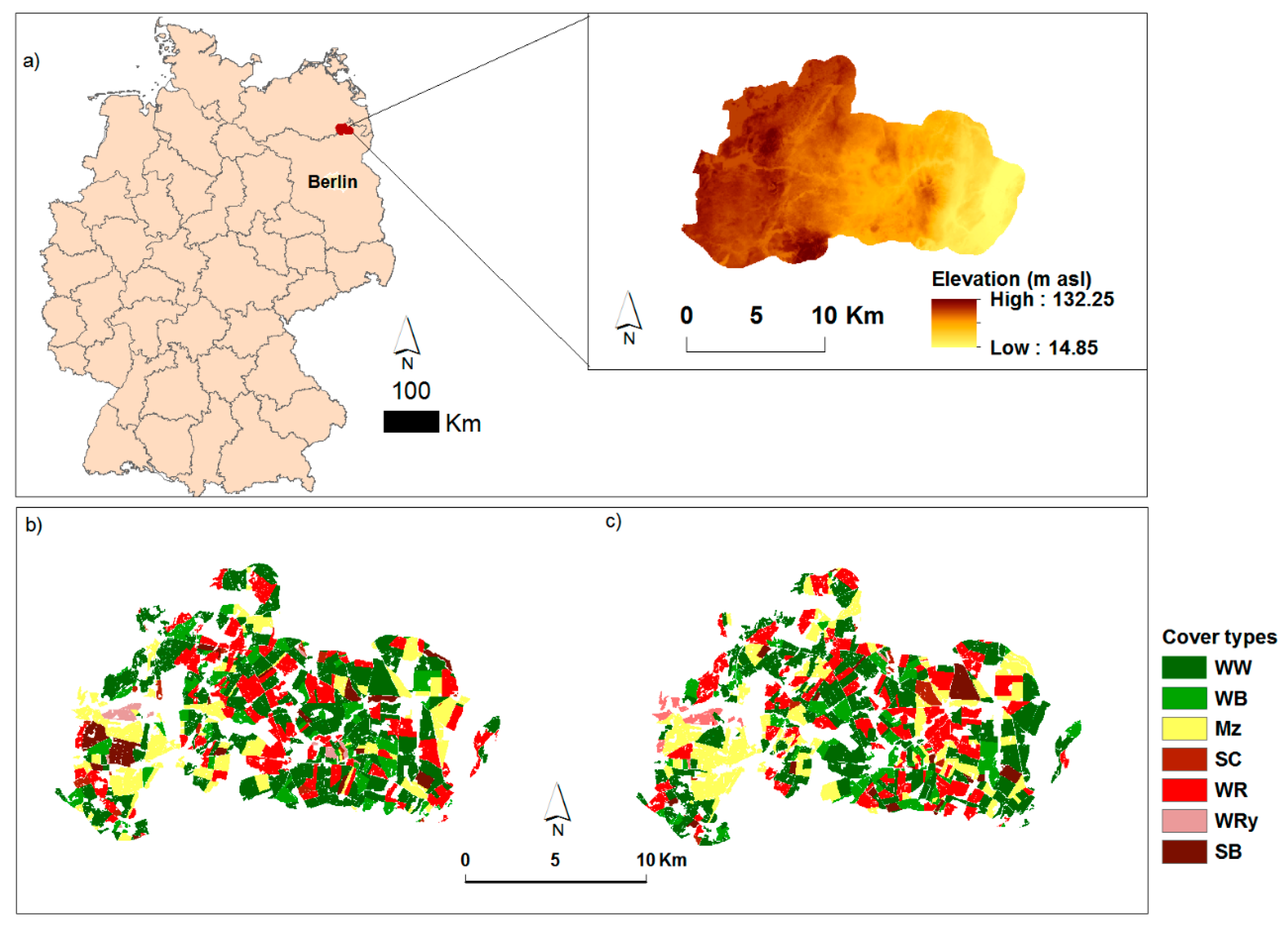
2.1. Study Area

The Uckermark district of the Brandenburg region (53°21″50′ N; 13°48″10′E ), in north eastern Germany, was the study area (Figure 1a). The land formation of the study region was shaped as a result of the advancement and cessation of glaciers during the last glaciations [30] resulting in moderately undulating topography with elevation ranging from 14 m to 132 m above sea level. The land formation process influenced the pedogenesis in the region, which caused the heterogeneity in soil types across different topographical forms [31,32]. The main soil type on hill tops and upper slopes ranges from slightly eroded Luvisols to Calcaric Regosols. The soils at mid slopes and on plateau primarily consist of Luvisol, Haplic Luvisol, while the depressions consist of Pseudogley (classified as Stagnosols, according to WRB-IUSS [33] soil types [31,32]. The climate of the region can be characterized as temperate and continental with an annual average air temperature ranging between 7.8 °C and 9.5 °C [34]. A mean annual precipitation of 460.2 mm was recorded between the years 1992 to 2016 at Grünow weather station [35]. Regarding the land use in the region, 75% is used for arable farming [30], predominantly covered by winter cereals, winter rape, maize, and sugar beet (Figure 1b,c).

2.2. Dataset and Processing

2.2.1. Satellite Imagery

Here, we combined Landsat 7 and 8 data with Sentinel 2 data in order to obtain temporally representative cloud free images. Time series of satellite observations (in total 30 images) Landsat 7 and 8 (using path 193, row 23) and Sentinel 2 (using tile ID 33UVV) data acquisitions from 2013 to 2016 were downloaded from United States Geological Survey (https://earthexplorer.usgs.gov/) and from the Copernicus Open Access Hub (https://scihub.copernicus.eu/dhus/#/home), respectively. In order to represent the different cropping stages (as depicted in Table 1), we included at least one image from each season of the given considered year. For analysis, scenes were selected with cloud cover of less than 30%. Most of the images covering the study area were cloud free and all images were atmospherically corrected. Cloud and snow cover masks (obtained along with the images) were used to exclude any cloud and snow-covered pixels from further analysis. With respect to the Landsat 7 data, the Scan Line Corrector failure affected less than 3% of the study area and this did not influence the result significantly, as indicated by a comparison of the NDVI values from two closely taken Landsat 7 and Landsat 8 images (see Appendix A Figure A1). Radiometric and phenological consistency between two temporally close Landsat 8 and Sentinel 2 scenes was checked via simple per pixel correlation analysis. A high correlation coefficient of 0.97 was determined between the mean values of agricultural parcels and no significant mean variation (p = 0.47) between the two data was observed (see Appendix A Figure A2).

2.2.2. Land Use/Land Cover Data

The IACS data provide high spatiotemporal resolution information on arable land use, crop type, field size and shape, and related aspects in a single vector dataset [37,38]. The IACS data from 2014 to 2016 were rasterized and sampled to 30 m resolution. As the focus of this research is on arable land, other land use types were excluded from the analysis. The major crops considered for the study are displayed in Figure 1b,c.

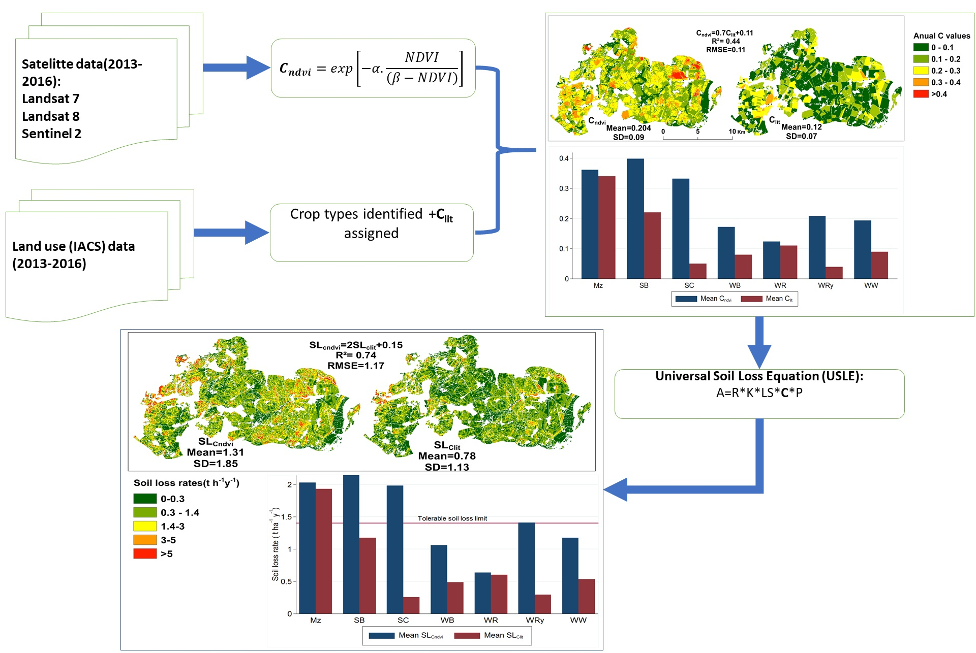
2.3. C Factor Value Estimation

In this study, periodic SLR values for each specific crop types, determined by the IACS data, were assigned from long term empirically measured SLR data, depicted in Table 1, as per DIN 19708 [39]. These SLR values were determined according to the corresponding cropping stages of individual crops considered (Table 2). Then, these values were weighted by their corresponding monthly average erosivity proportion values (Table 2, 2nd row) adapted from [40], to result in monthly C factor values (ClitM). Finally, the annual literature-based C values (Clit) of each crop type were assigned from Deumlich et al. [36], a regional average value for northeast Germany.
In order to estimate C values using NDVI, the index was computed for each image as described by Tucker [41]:
N D V I = ( N I R R e d ) ( N I R + R e d )
The NDVI can take values between1 and +1 (soil: usually 0.1–0.4, vegetation: 0.2–0.9) and—if observing vegetation—is an expression of the underlying LAI and photosynthetic activity: the higher the NDVI value, the “greener” the vegetation (coverage), indicating that photosynthetically active vegetation is reflecting much of the near-infrared radiation while absorbing the visible range of the spectrum. The NDVI-based C value (Cndvi) was calculated for each image [42]:
C n d v i = e x p [ α · N D V I ( β N D V I ) ]
where α and β are empirical (dimensionless) fitting parameters. Good correlations were obtained when using a value of 2 for α and 1 for β [42]. This particular equation has been used in several studies worldwide to calculate C values [4,17,43,44,45,46]. Since the equation was developed using daily images by comparing against monthly C factor values, it allows us to calculate monthly (CndviM), and annual C values (Cndvi) by aggregating the average values of the scenes accordingly. Finally, the NDVI-derived C factor outputs from Sentinel 2 (at 20 m resolution) were re-sampled to 30 m resolution using the nearest neighborhood method, to maintain the original values, while aligning with the Cndvi from Landsat 7 and Landsat 8 data for subsequent analysis.

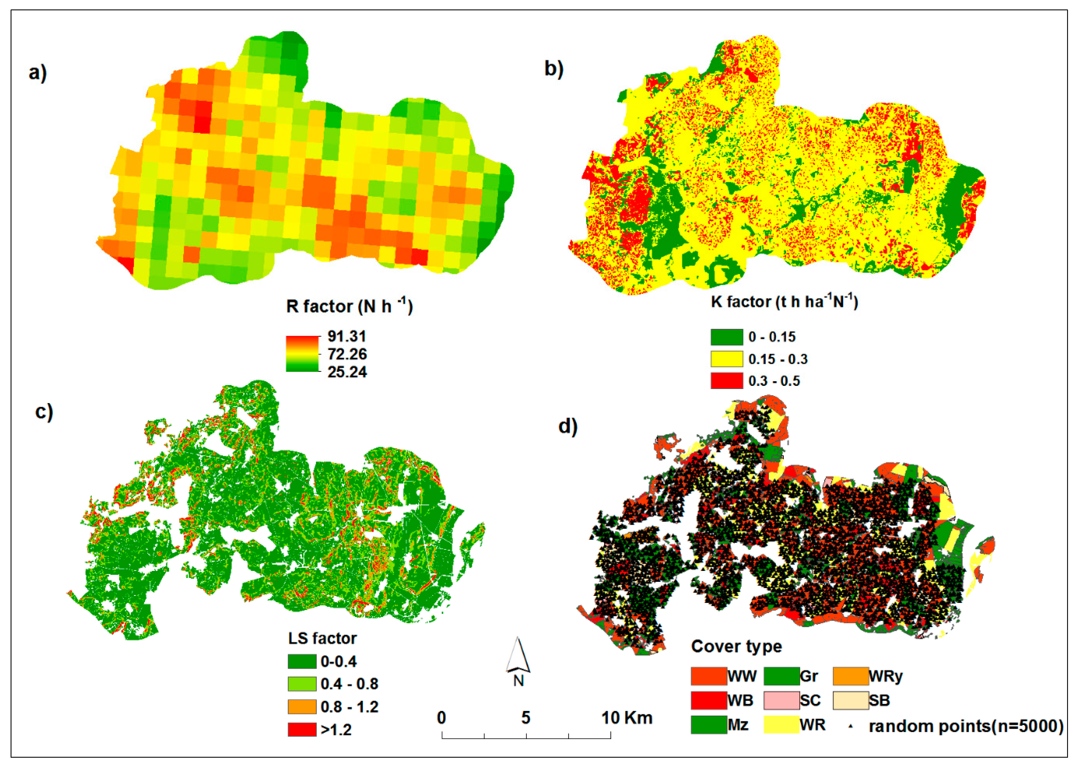
2.4. Soil Erosion Prediction

Potential soil erosion risk was predicted by employing the USLE (Equation (4)) [6]. In Germany, employing the USLE (or an adapted form of the equation named “ABAG”) to predict soil erosion risk by water is a recommended practice, especially when precise soil loss rates are not required but the demand is rather for trends and patterns of soil erosion for the purpose of agricultural land management [47,48].
A = R · K · L · S · C · P
where: A is the predicted average annual soil loss in t ha−1 y−1. R (N h−1, Newtons per hour, a commonly used unit in Germany that can readily be converted to MJ mm ha−1 h−1 by multiplying it by a factor of 10) is calculated as the mean annual sum (Figure 1a) of the product of a maximum 30 min rainfall intensity (I30) and energy (Ei) of a rainfall event (Equation (5)) [6,39]. Eight years of radar rainfall data (RADOLAN from 2006 to 2013), with 5-min temporal and 1 × 1 km2 spatial resolution, obtained from the German Weather Service (DWD), were used to calculate EI30 according to Wischmeier and Smith [6] as:
E I 30 = i = 1 n ( E i ) I 30   { E i = ( 11.89 + 8.73 l o g I i ) P i 10 3 ,   f o r   I i 0.05   m m / h E i = 0   f o r   I i < 0.05   m m / h E i = 28.33 P i 10 3   f o r   I i > 76.2   m m / h
where i denotes the ith rainfall event, Ei is the kinetic energy (KJ m−2) of the ith rainfall event, Pi is the total amount of rainfall (mm) of the ith rainfall event, and Ii is the rainfall intensity of the ith rainfall event (mm h−1). Utilizing radar weather data for rainfall erosivity calculation and erosion prediction has been found to be adequate [49]. K (Equation (6)) is the soil erodibility factor (t h ha−1 N−1) calculated according to Wischmeier and Smith [6] using data available from the German Soil Appraisal “Bodenschätzung” (Figure 2b).
[ 2.1 10 4 ( 12 a ) M 1.14 + 3.25 ( b 2 ) + 2.5 ( c 3 ) ] / 100
where M is the particle size parameter, a is the percentage of organic matter, b soil structure parameter, and c is the soil profile permeability class. The topographic factor LS (Figure 2c) represents the slope length (L) calculated according to Hickey [50] and slope steepness (S) calculated as per Nearing [51], using a 5-m digital elevation model (DEM). The S and L (Equations (7) and (8)) are calculated as:
S = 1.5 + 17 / [ 1 + e ( 2.3 6.1 s i n θ ) ]
L = ( l / 22.13 ) m
where θ is the slope angle, l is the cumulative slope length calculated according to Hickey [50], and m is slope contingent variable, which takes a value of 0.5 if the slope angle is greater than 2.86°, 0.4 on slopes ranging between 1.72° and 2.86°, 0.3 on slopes between 0.57° and 1.72°, and 0.2 on slopes less than 0.57°. The dimensionless C factor is the ratio of soil loss under known vegetation cover to that of bare soil. The C factor is the main manipulation factor in this study and potential soil erosion prediction is done using both Cndvi (Equation (3)) and Clit values. For the soil-protecting practice factor, P, a value of 1 was used because no support practice exists for the study region.

2.5. Statistical Analysis

In order to address the second objective, quantifying the influence of biophysical variables on Cndvi values, a sample of 5000 spatially balanced random points (Figure 2d), constrained within the arable land of the study area (using ArcMap, v10.2.2) were generated and further used to extract multi-values from the considered biophysical explanatory variables (Table 3). The means and standard deviations of the sample values were compared with the corresponding values from the entire study area, to check the representativeness of samples, using a t-test analysis (see Appendix B Table A1). Multiple linear regression analysis was performed using the extracted values against the corresponding Cndvi values through R (package “stats”) software version 3.6.0 [52].
The biophysical variables used in the study (Table 3) are topographic features such as slope steepness (degree), slope shape, slope position, slope aspect, edaphic conditions of the area (proxied through K factor values), and seasonal and crop type variation. A digital elevation model (DEM) of a 5-m resolution (Figure 1a), derived by airborne laser scanning, was used for the computation of the topographic features. Slope position and slope shape were calculated through the topographic positioning index [33]. Soil properties of the study area are proxied by soil erodibility condition in the form of the K factor values for the reasons that K is calculated by taking into account the soil texture, soil organic matter content, and particle size distribution of the area [39], in addition to its applicability in quantitative analysis and explanation [53].
As the data set features some categorical variables such as slope shape, slope position, crop cover type, the multiple regression model is expressed as:
y = β 0 + β 12 α 2 + β 13 α 3 + X β 2 . + ε
where β12, β13 represent the coefficient expression of the given categorical variables, α2 and α3, respectively, as compared with a reference variable (α1 where its coefficient β11 is set to 0), α2 and α3 represent categorical variables, X is a non-categorical variable, and β2 is the coefficient for the non-categorical variable [54]. The categorical expression for the different crop types was performed by taking winter wheat as a reference crop, because winter wheat occupied a large proportion of the study area in all the considered years. For slope shape and slope position, flat land and the slope summit categories were taken as reference categorical variables, respectively (Table 3). Changing reference variables does not make any statistical difference in the final output of the regression analysis; rather, it facilitates a simpler comparison between variables.
Finally, the performances of satellite-based C factor estimation and soil loss prediction were assessed by employing root mean square error (RMSE) computation expressed as:
R M S E C = 1 n ( C l i t C n d v i ) 2 n   and   R M S E S L = 1 n ( S L C l i t S L C n d v i ) 2 n
where SLClit is the potential soil loss predicted using Clit, SLCndvi is the soil loss predicted using Cndvi, and n is the number of pixels coinciding in the analysis. Furthermore, the erosion prediction accuracy of using the USLE model in general, or through the two different C values (SLcndvi and SLclit) in particular, was discussed by comparing the model output with long term (from 1982 to 1996) average soil erosion values measured from field experiments at the Holzendorf (Latitude 53.386818, Longitude 13.780225) research station [55]. The experimental set up and measured erosion values can be referred from Deumlich et al. [55].

3. Results and Discussion

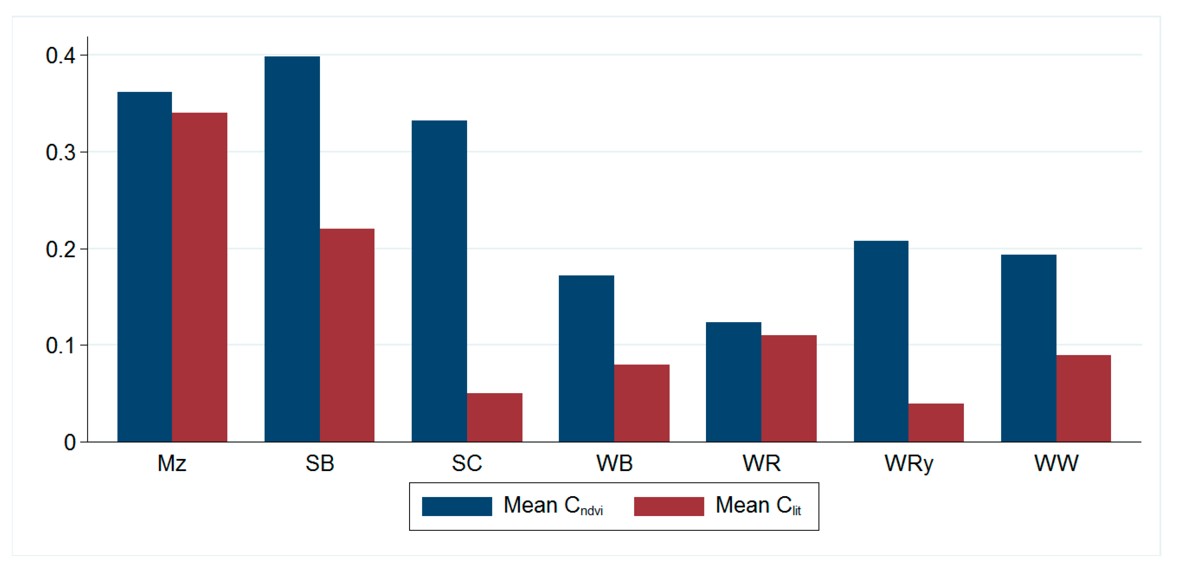
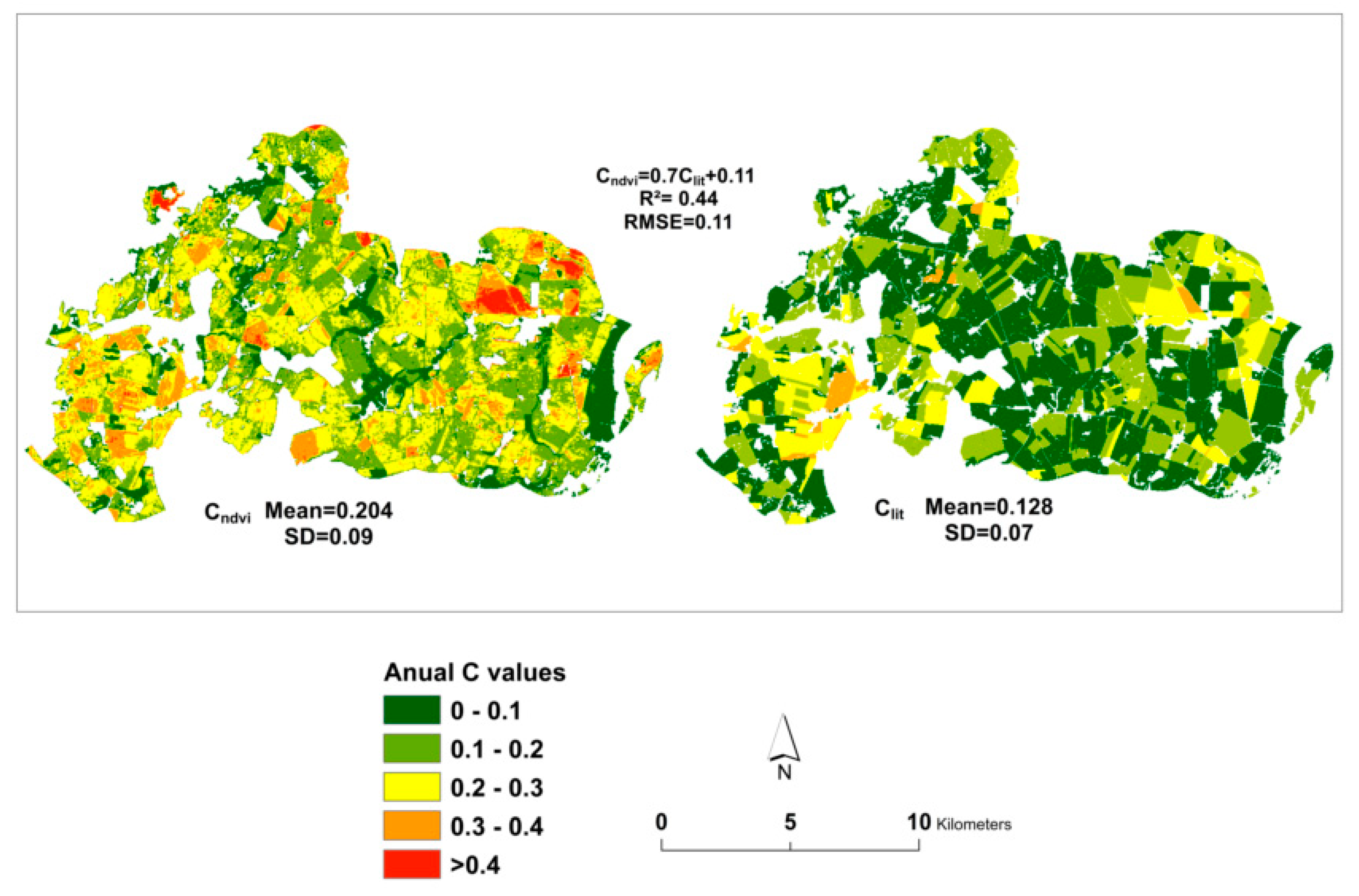
3.1. Comparisons between Cndvi and Clit Estimation

Table 4 indicates the spatial correlation between monthly CndviM and ClitM values of the entire landscape. Better correlation between CndviM and ClitM values was observed in images taken in the months between spring and mid-summer, with the highest correlation coefficient (r = 0.93) computed on the image taken on 09 May 2016. The lowest correlation, however, was observed in the months of late summer and autumn, while in a few of the images a negative relationship between CndviM and ClitM values was observed. In particular, August, September, and October were the months where the highest RMSE was computed. This can be due to variations in the vitality of many winter-sown crops during these periods of the year; NDVI-based C factor values, as opposed to the SLR based values, which mainly reflect the function of the protective ability of the crops in question, are highly influenced by the vitality of the plants rather than the crop-cover percentage [20,42]. In these periods, large areas of the landscape (see Figure 1b,c for proportion of crop cover) are expected to have either maturing and senescing crops (e.g., August) or early-emerging and less-ground covering crops (e.g., October), in which case the NDVI values were lower (Appendix A Figure A3), in turn resulting in elevated monthly CndviM values. One possible solution could be to incorporate yellow vegetation indices such as normalized difference tillage index (NDTI), and normalized difference senescent vegetation index (NDSVI), in the process of formulating the C factor equation, for future in order to improve the C value estimation across all seasons [7]. Overall, lower RMSEs were consistently computed on images taken during the month of June in each of the three years considered.
When comparing CndviM values of individual crop-cover types with corresponding ClitM values, a better estimation for winter crops was observed in spring months and, to a lesser extent, in the beginning of summer months (April to the mid of June), while for spring sown crops, better estimation was obtained on images taken exclusively in summer months (June to September) of the year (Appendix A Figure A3), which closely coincided with the expected growth patterns of the crops in the study region. This can indicate the applicability of the IACS data combining with remote sensing images to capture the temporal variability in C value determination. In general, there was a tendency of high C value estimation using NDVI as a tool compared with ClitM value estimation in all the months considered. Almagro et al. [56] also reported that C values estimated via the NDVI (employing Equation (3)) resulted in over estimation of C factor values compared with plot scale literature values in tropical conditions.
When it comes to annual C value computations, which is the required input factor for the USLE model, average Cndvi calculations resulted in higher values compared with empirical Clit values specifically for winter cereals and summer cereal (Figure 3). The highest discrepancies were observed on parcels covered with SC (85%) and WRy (80%) while the lowest discrepancy, around 5% and 5.3%, appeared to be on parcels covered with WR and Mz respectively. Bargiel et al. [57] also noted that C factor determination through remote sensing application gives better accuracy for summer crops than winter grains (without considering WR) in a similar condition in Poland. Annual C values of Mz and WR can be captured with a better accuracy as indicated by the least discrepancy estimated here. Comparatively, the NDVI-derived C value estimation also performed better for SB compared with winter and summer cereals. This could be explained to some extent to the variation in patterns of foliar orientation of these crops. WR, Mz and SB categorized as plagiophile and planophile, respectively, while most cereals categorized as erectophile crops behave differently with respect to canopy spectral reflectance [58]. Erecophile canopy, leaves arranged in vertical manner, could trap reflected radiation within the canopy and reduce the NDVI while the opposite is true for planophile canopy orientation types [29].
Figure 4 depicts the spatial distribution of C values computed with the two methods. The classification of the study area indicates discrepancy between the two C value estimations. In case of Clit, areas classified with C values below 0.1 accounted for 51% of the entire landscape, while Cndvi values of the same category was computed on just 13% of the study area. However, proportions of the landscape falling in the category between 0.1 and 0.2 were comparatively close to each other: around 33% with Cndvi and 31% with Clit. One peculiar thing about the Cndvi calculation is that it produced continuous and spatially varying C factor values within individual parcel as opposed to a discrete representation by the Clit. This obviously can indicate the potential of the NDVI-based C factor estimation for capturing spatially explicit variation of different cover types for possible implication of spatially explicit erosion prediction models, provided that the appropriate adjustments are made (see Section 3.3 and Section 3.4 for a further discussion of adjustments).

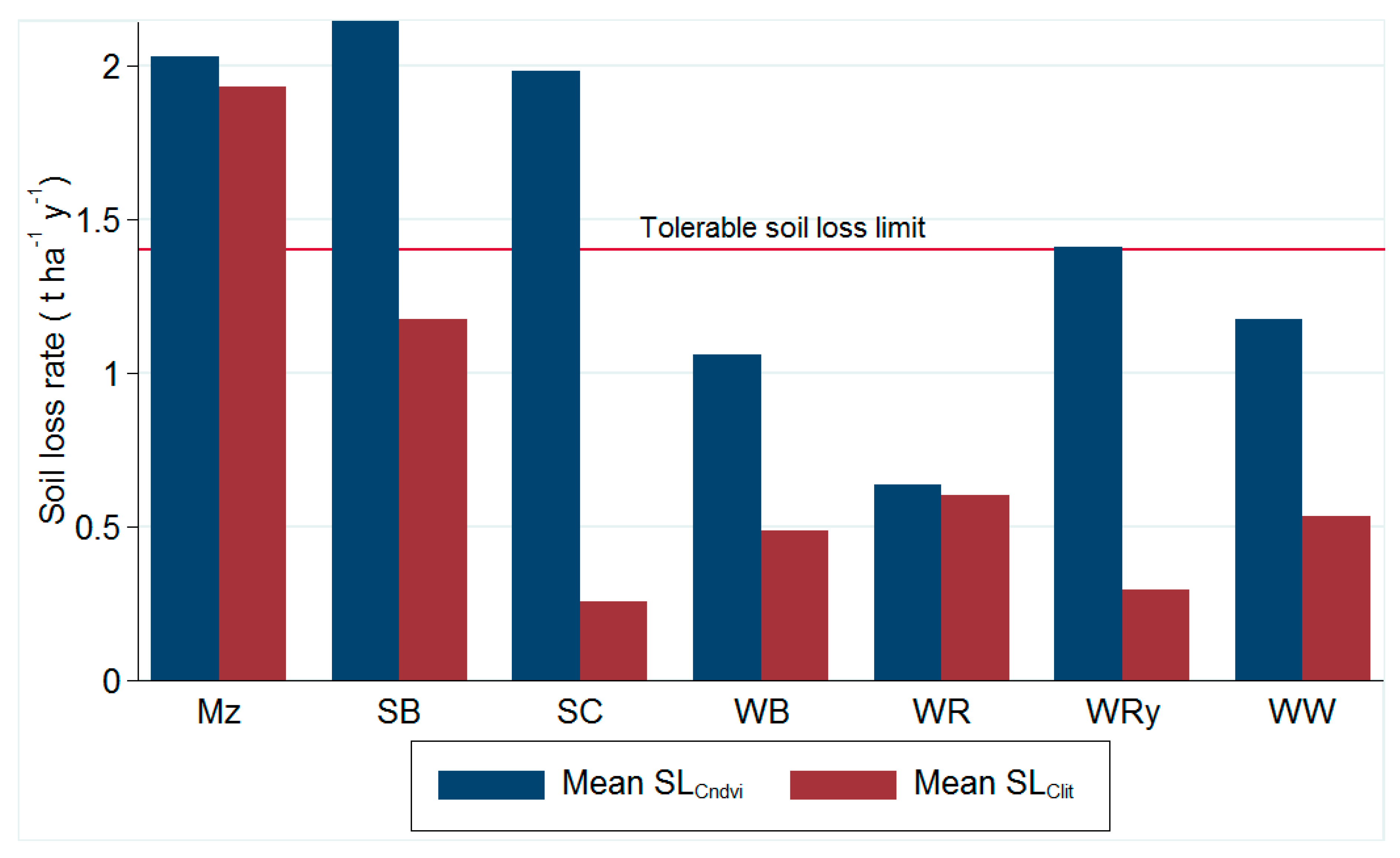
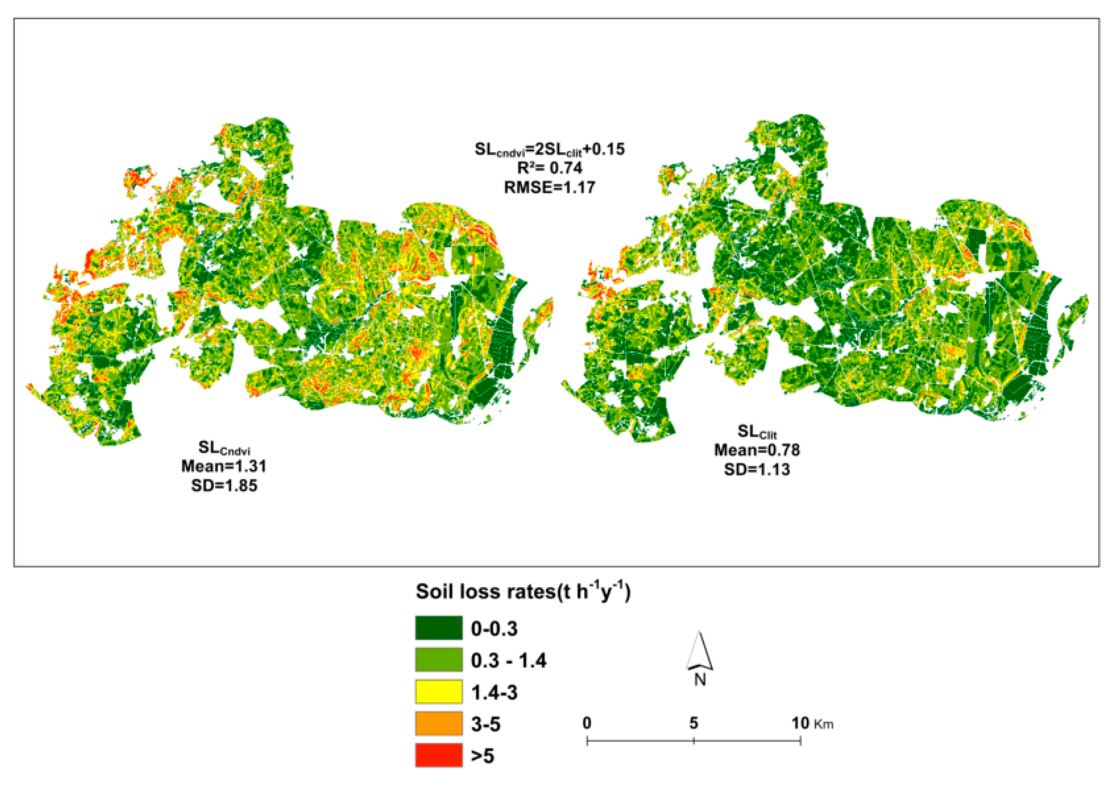
3.2. Potential Soil Erosion Risk Prediction Using the Two C Estimation Methods

Subsequent modelling of potential soil erosion risk reflected the variation of C factor values. The three-year average annual potential soil loss rates predicted using Clit (SLclit) resulted in values falling below the maximum tolerable soil loss limit (rates < 1.4 tha−1y−1) [59] set for European conditions, as per Verheijen et al., for all crops, except Mz (Figure 5). On the other hand, in the case of SLcndvi, only winter-sown crops fall below this limit. All the spring sown crops, however, predicted high potential soil loss rates above the tolerable limit using Cndvi values inputted in the USLE model. WR- and Mz-covered parcels gave quite close soil loss rates. In recent years, the coverage of bio-energy Mz and WR in the study region has witnessed an incremental trend, which in turn requires to understand the associated environmental impact at wider scale [34,60]. In this regard, we have indicated that remotely sensed data can be reliable input for various environmental monitoring and modelling activities.
Spatially, the potential soil loss rates predicted using the two different C factor inputs revealed an RMSE as high as 1.17 t ha−1 y−1, which was below the maximum tolerable soil erosion limit (Figure 6). However, the spatial distribution of the potential soil erosion risk varied greatly. For example, the proportion of the landscape classified below the maximum tolerable soil loss limit in the case of SLcndvi was close to 85%, while the same classification in the case of SLclit accounted for close to 70%. In aggregate, the soil loss rate obtained by employing Cndvi as a C-factor input for the USLE model resulted in two times higher prediction than when using Clit.
The accuracy of the USLE model in general was assessed by comparing the potential soil loss rates against the measured long-term average annual soil loss rates. The measured values ranged from 0.5 to 5 t ha−1 y−1; the lowest value measured from WRy mono cultivation, while the highest was measured from continuous fallow plots. The SLclit gave a comparatively closer estimation than the SLcndvi, with a three-year average of 1.11 t ha−1 y−1 predicted from the WW and WR sequenced parcels located near the surrounding of the Holzendorf experimental station (see Appendix A Figure A4). The potential soil loss rate predicted using Cndvi, however, yielded an average value of 2.13 t ha−1 y−1 for the same cropping sequence. The closest comparison here is WRy monoculture. Given the fact that rainfall erosivity increased over the recent years in the study area [61] and the variation in C values of the crop types, WRy had low C factor values compared to WR and WW [36], the model output from SLclit can be fairly taken as accurate. SLcndvi erosion prediction, on the contrary, overestimated (close to double) the erosion rate as compared to SLclit. However, SLcndvi can improve spatially explicit identification of soil erosion risks as opposed to SLclit. This can be inferred from the relatively higher coefficient of variation (CV) of 91% computed in the case of SLcndvi as opposed to 84% in SLclit (Appendix A Figure A4). This can indicate the potential of utilizing NDVI-based C factor estimation for physically based erosion models such as SWAT.

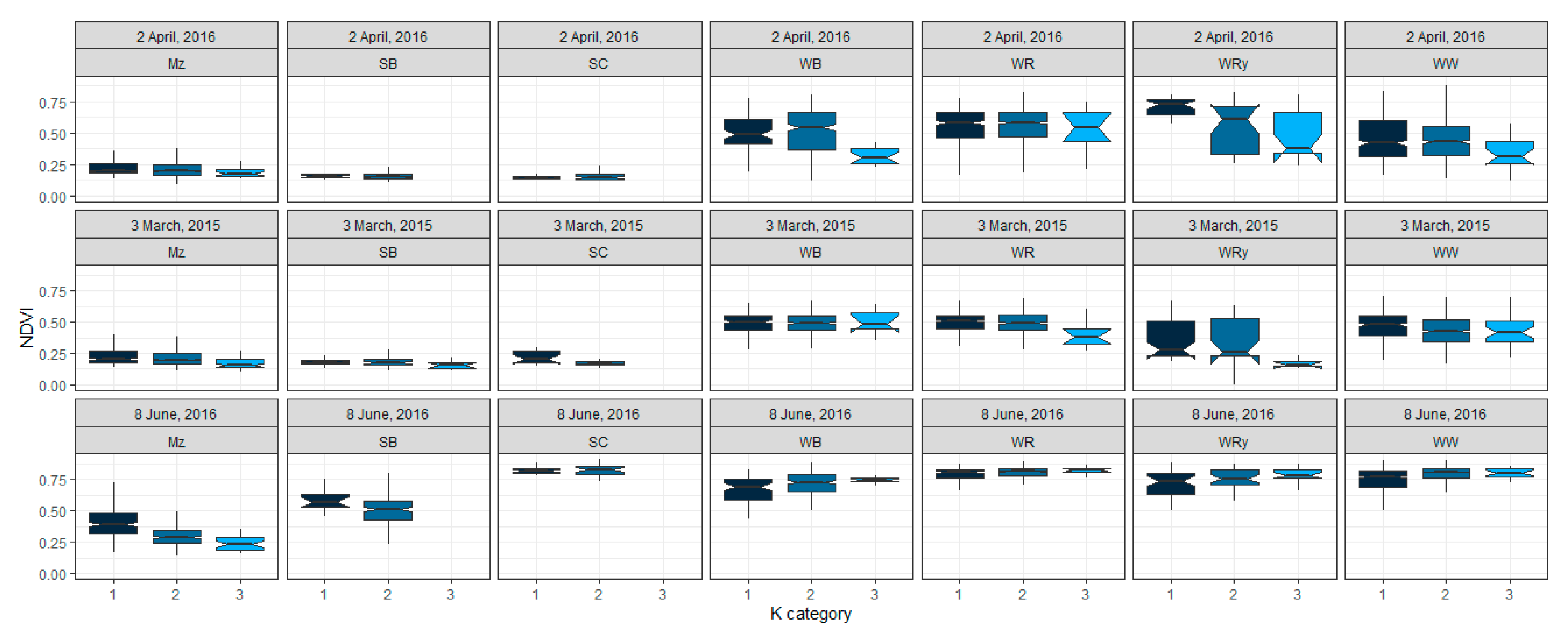
3.3. Influence of Soil Heterogeneity on Cndvi

Multiple regression analysis revealed that C values estimated from the vegetation index were affected by the biophysical variables considered (Table 5). The sensitivity of Cndvi estimations to soil background variation can be explained through the spatial variability of soil erodibility (K) values in the study area. This is in agreement with the findings of Wang et al. [53], who reported that the spatial variability of K factor values can be represented by Landsat TM band 7 variability. In the present study, an increase in the value of soil erodibility resulted in an invariable incremental change in the values of Cndvi, although the magnitude varied in different months of a year. Sizeable impact, in terms of magnitude, was observed during spring and the beginning of the summer months. These are the periods when ground cover contrast is expected to be high. Huete et al. [62] indicated that the influence of soil background on plant canopy spectral reflectance is more pronounced on soils with 75% ground cover than on either fully exposed or less ground-covered soils.
The variation in Cndvi values resulting from soil background heterogeneity could be well explained through the Red and Near Infrared (NIR) bands reflectance variation, particularly on the highest soil erodibility categories (Figure 7). Soil characteristics such as soil texture, organic matter content and surface roughness are reported to influence the spectrum properties of a landscape [26]. Remarkably consistent variations in the reflectance values of both Red and NIR spectrum were observed on soils with an erodibility class of greater than 0.3 t h ha−1 N−1. The higher the K value, the higher the red reflectance, but the lower the NIR reflectance, which could result in low NDVI values, as NDVI is the normalized ratio of the two bands. This can be attributed to the fact that soils with lower erodibility characteristics have relatively higher organic matter contents, which in turn gives the soils a darker color. Soil with a darker color are reported to have higher greenness value than brighter colors [62]. This could, to a degree, explain how soil erosion risk predicted using Cndvi (SLcndvi) yielded higher values, as opposed to SLclit, because of the compounding effect of the K and Cndvi values in the USLE model (Figure 6).
The Cndvi values responded differentially to soil background heterogeneity across different crop-cover types and seasons; during winter and spring, the association of Cndvi with soil condition was pronounced on lands covered with winter sown crops (with the exception of WR) more during summer on the lands covered with spring sown crops (Figure 8). This could be explained in relation to the growth stages of the crops in question, whereby during winter and spring periods, parcels covered with winter-sown crops, or with spring sown crops during the summer period, would exhibit mixed spectral characteristics of both the exposed soil and vegetation of not fully-closed canopies. However, as time proceeded, the canopies of the respective crops in the respective seasons would fully cover the parcels; hence, the radiometric signal is less dominated by the soil background reflectance [26].
The least pronounced impact of heterogeneous soil background reflectance on parcels covered with WR can be explained by the nature of the architectural orientation of the crop canopy. WR, plagiophile canopy, is reported to have a higher plant area index compared with WW (belonging to erectophile), even at the same phenological stage [58]. This can also be inferred from Figure 8 in our study, where, despite both WR and WRy being expected to cover around 75% of the ground in the images dated 02 April 2016 (Table 2), their NDVI values and response to K value categories varied significantly. Land surfaces covered with WR showed no significant response to soil heterogeneity and had comparatively higher NDVI values consistently (Figure 8). However, a further investigation with ground measurements needs to be done to further understand the relationship of crop canopy structure and C factor value estimation for future.
Other spectral indices such as the enhanced vegetation index (EVI) and soil adjusted vegetation index (SAVI) have been developed to increase sensitivity to changes in biomass while reducing the impact of soil background noise on vegetation spectral property [63]. However, these indices may introduce a higher sensitivity to topographic variability, which might take effect in rugged/mountainous areas [19]. Therefore, consideration of all biophysical variables in calibrating spectral indices for the purpose of environmental monitoring such as erosion prediction remains imperative.

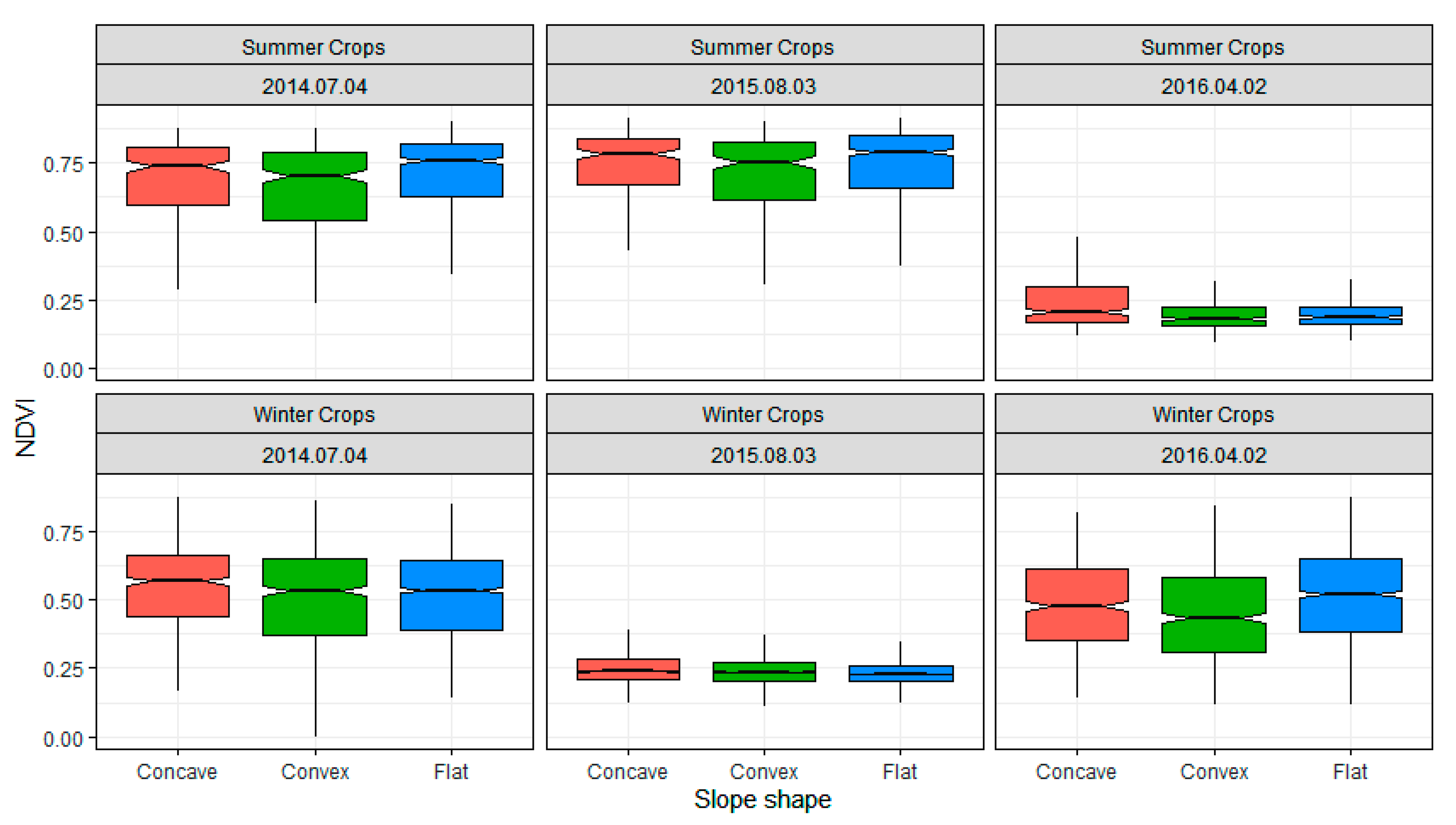
3.4. Influence of Topographic Features on Cndvi

The regression analysis also revealed that Cndvi values showed consistently significant response to varying slope shapes of the landscape (Table 5). Slope aspect, however, did not show any significant relationship with Cndvi estimation. Matsushita et al. [19] also reported that topographical features such as aspect do not exhibit significant influence on band ratio indices such as NDVI. Although slope steepness showed a significant impact on Cndvi values in just two images, the regression coefficient was a very small number close to zero; hence, it is not discussed here.
Convex shaped slope, as compared to flat slope, demonstrated significant incremental implications on Cndvi values, with the highest coefficient of 0.05 (P < 0.01; R2 = 0.57) predicted on the image taken on 02 April 2016 (Table 5). Concave shaped slope, on the other hand, revealed to have a negative relationship with the estimated Cndvi values compared with the flat slope. The impact of concaved slope on Cndvi values was predominantly observed on images taken from the end of June to August. This can be due to the indirect influence of topographic attributes on vegetation status, as concave slopes, located towards the depression parts of the study area [31], are most likely assumed to be cooler in summer as compared to flat land; hence, the crops could senescence late and could remain vital for a longer time. In addition, this could also be due to the fact that drainage patterns vary with slope shape, bearing implications on soil moisture conditions of a landscape, in such a way that concave slopes produce less runoff compared with flat and convex slopes [64,65]. In the study area the different slope shapes also have a complex interaction with prevailing soil types, due to erosion and deposition processes [55]. Concave part of slope act as depositional sites while the convex parts of the slope are dominated by eroded soils. These attributes of the landscape could also play a role in the status of crop growth and subsequently in Cndvi estimates.
Convex slopes seemed to increase Cndvi value estimations, with considerable magnitude recorded on images taken in winter and early springtime. The impact of varying slope shape varied with crop growth stages (Figure 9). During springtime (e.g., image 02 April 2016), the impact of slope shape on the NDVI values was more evident for winter crops, parcels covered with summer crops exhibiting a typical NDVI value for bare soil. In the middle of the summer season (04 July 2014), when most winter crops were approaching maturity stage, the impact of slope shape, specifically concave slope, exerted an influence on the NDVI values of winter crops. Towards August (03 August 2015), the influence of slope shape variation was entirely limited to summer crops because winter crops had most likely been harvested. In general, while using NDVI for C factor estimation, considerations must be taken into account to accommodate for land formation influence on the status of the vegetation.

4. Conclusions

In the present study, we used annually updated high resolution land use data, high resolution multi-temporal remote sensing data, and topographic and soil attribute data to quantify deviations between NDVI based C value estimations (Cndvi) and traditional literature-based C values (Clit) in addition to quantifying the sensitivity of Cndvi estimation in large agricultural landscape. Combining these datasets enhanced the quantification of the discrepancies between Cndvi and Clit. A higher discrepancy was observed among winter cereals than summer crops. The discrepancy in C values between Cndvi and Clit was also found to be season dependent with a closer relation observed in early spring to midsummer, with consistently lowest RMSE values for data from June. Subsequently modelling soil erosion using Cndvi as input factor could yield higher annual mean soil loss rate values, while it could potentially improve the spatially explicit erosion risk identification.
In quantifying the sensitivity of Cndvi, the K factor was reliable and consistent to explain the response of Cndvi values to soil background heterogeneity. Higher erodibility condition, particularly K values above 0.3 t h ha−1N−1, was associated with significantly higher Cndvi value estimation: up to 0.28 times higher. It was also indicated that the relationship between Cndvi estimates and heterogeneous soil conditions can be further dissected according to the canopy structure of different crops; namely, Plagiophile crops, found to be less response to background soil conditions than erectophile types. Identifying land cover type to specific species level, by coupling remote sensing data with the IACS data, allowed quantifying the sensitivity of Cndvi to soil background heterogeneity in relation to crops’ growth stage.
The research also indicated that variable slope shape can be reliably used in quantifying the sensitivity of Cndvi estimates to topographical variations. Convex and concave slopes were found to have opposite implications on Cndvi values, in that the concave slope was associated with lower Cndvi values (up to 0.01 times smaller values compared with flat slope), while the convex slope had an incremental implication (up to 0.05 times higher values compared with flat slope). The impact of different slope shapes also showed variability according to season; a more evident implication of the concave slope was in late summer, while the association of convex slope with higher Cndvi values spread from spring to the beginning of autumn. The results can be useful inputs in improving the capacity of Cndvi estimation for landscapes as complex as the present study region. In addition, utilizing remote sensing data for the purpose of capturing spatiotemporal variation in C factor determination and subsequently serving as input factor for process-based soil erosion modelling can be enhanced by considering the quantified sensitivity of Cndvi estimations. The information obtained from such modelling practice could also benefit the evaluation of several agricultural land management options in large and complex agricultural landscapes efficiently and more accurately.
For future research, we suggest to explicitly study C factor determination, including spatially distributed climatic data along with yellow vegetation indices in order to improve the applicability and transferability of the Cndvi method to regions with similar conditions.

Author Contributions

Conceptualization, D.A.A., D.D. (Detlef Deumlich), and B.Š.; Data curation, D.A.A. and D.D. (Daniel Doktor); Formal analysis, D.A.A; Investigation, D.A.A. and D.D (Detlef Deumlich); Methodology, D.A.A., D.D. (Detlef Deumlich) and D.D. (Daniel Doktor); Resources, D.D. (Detlef Deumlich) and B.Š; Supervision, D.D. (Detlef Deumlich) and B.Š.; Writing—original draft, D.A.A.; Writing—review and editing, D.A.A., D.D. (Detlef Deumlich), B.Š., and D.D. (Daniel Doktor). All authors have read and agreed to the published version of the manuscript.

Funding

This research received no external funding.

Acknowledgments

The first author is a recipient of the Czech Republic government scholarship for their PhD study. This study is part of their PhD work. The first author also benefited from financial assist from Palacký University Olomouc through the grant (IGA_PrF_2020_020) and from the project of the National Agency for Agricultural Research of the Czech Republic No. QK1810233. We would also acknowledge ZALF in Müncheberg for the first author’s research stay. Finally, we acknowledge Horst H. Gerke, from ZALF, for his helpful comments and editing works on the manuscript.

Conflicts of Interest

The authors declare no conflict of interest.

Appendix A

Figure A1. Comparison of NDVI values between two closely taken images from Landsat 7 and Landsat 8 satellites, indicating comparably similar distribution and statistics.
Remotesensing 12 01136 g0a1
Figure A2. Mean and variance NDVI comparisons between Sentinel 2 and Landsat 7 images; there was no significant difference between the means (p = 0.47) in these two closely sensed data. Correlation coefficient was r = 0.97. Values are the averages of each parcel (n = 1130 parcels) from 2016 IACS data extracted using the R package “raster.”
Remotesensing 12 01136 g0a2
Figure A3. NDVI variation across different crop cover types in the study area. In June, almost all crop covers had a median NDVI > 0.5. As the summer progressed, winter-sown crops such as WRy, WB, and WW showed a decline in median NDVI values, which could elevate the Cndvi values of the study area.
Remotesensing 12 01136 g0a3
Figure A4. Three years average potential soil erosion rate in a catchment around Holzendorf experimental station: (a) land cover type from 2014 to 2016 cropping year identified through the IACS data; (b) and (c) erosion predicted using Clit (SLclit) and using Cndvi (SLcndvi), respectively. Compared to the long-term experimental results, which ranged from 0.5 to 5 t ha−1 y−1, the values predicted using the USLE can fairly be taken as representative.
Remotesensing 12 01136 g0a4

Appendix B

Table A1. Data comparison between randomly extracted data points (samples) and the whole scene statistics (population). The t-test indicated no statistical difference between the two groups (p = 0.92, t value = 2.0 for the means; and p = 0.99, t value = 2.0 for standard deviations).
VariablesMeanStandard Deviation
Sample (n = 5000)PopulationSample (n = 5000) Population
Slope2.522.581.952.14
K value0.20.190.070.07
LS factor0.360.370.380.40
Cndvi by scene dates
29 October 20130.210.190.210.21
10 February 20140.260.250.200.19
30 March 20140.140.130.210.20
1 May 20140.170.140.250.23
18 June 20140.070.070.120.11
4 July 20140.120.110.150.15
13 August 20140.250.240.240.24
6 September 20140.320.310.270.27
8 October 20140.240.230.230.23
17 March 20150.290.290.210.20
25 March 20150.220.210.190.18
10 April 20150.160.150.220.21
5 June 20150.120.100.230.21
13 June 20150.090.080.170.16
4 July 20150.110.110.140.14
7 July 20150.120.110.140.14
3 August 20150.380.370.250.25
3 October 20150.300.290.250.25
27 October 20150.280.270.240.24
31 December 20150.210.20.220.22
2 April 20150.280.260.250.24
22 April 20150.210.180.260.25
2 May 20150.220.170.300.28
9 May 20150.210.160.300.28
12 May 20150.200.160.280.26
8 June 20150.090.080.170.17
23 June 20150.060.060.110.11

References

  1. Pimentel, D.; Burgess, M. Soil erosion threatens food production. Agriculture 2013, 3, 443–463. [Google Scholar] [CrossRef] [Green Version]
  2. Šarapatka, B.; Bednář, M. Assessment of potential soil degradation on agricultural land in the Czech Republic. J. Environ. Qual. 2015, 44, 154–161. [Google Scholar] [CrossRef] [PubMed]
  3. Borrelli, P.; Robinson, D.A.; Fleischer, L.R.; Lugato, E.; Ballabio, C.; Alewell, C.; Meusburger, K.; Modugno, S.; Schütt, B.; Ferro, V.; et al. An assessment of the global impact of 21st century land use change on soil erosion. Nat. Commun. 2017, 8, 2013. [Google Scholar] [CrossRef] [PubMed] [Green Version]
  4. Alexandridis, T.K.; Sotiropoulou, A.M.; Bilas, G.; Karapetsas, N.; Silleos, N.G. The effects of seasonality in estimating the C-Factor of soil erosion studies. Land. Degrad. Dev. 2015, 26, 596–603. [Google Scholar] [CrossRef]
  5. Schönbrodt, S.; Saumer, P.; Behrens, T.; Seeber, C.; Scholten, T. Assessing the USLE crop and management factor C for soil erosion modeling in a large mountainous watershed in Central China. J. Earth Sci. 2010, 21, 835–845. [Google Scholar] [CrossRef]
  6. Wischmeier, W.H.; Smith, D.D. Predicting Rainfall Erosion Losses—A Guide to Conservation Planning; U.S. Department of Agriculture: Washington, WA, USA, 1978.
  7. Feng, Q.; Zhao, W.; Ding, J.; Fang, X.; Zhang, X. Estimation of the cover and management factor based on stratified coverage and remote sensing indices: A case study in the Loess Plateau of China. J. Soils Sediments 2018, 18, 775–790. [Google Scholar] [CrossRef]
  8. Gyssels, G.; Poesen, J.; Bochet, E.; Li, Y. Impact of plant roots on the resistance of soils to erosion by water: A review. Prog. Phys. Geogr. 2005, 29, 189–217. [Google Scholar] [CrossRef] [Green Version]
  9. Arnold, J.G.; Srinivasan, R.; Muttiah, R.S.; Williams, J.R. Large area hydrologic modeling and assessment Part I: Model development. J. Am. Water. Resour. Assoc. 1998, 34, 73–89. [Google Scholar] [CrossRef]
  10. Neitsch, S.L.; Arnold, J.G.; Kiniry, J.R.; Williams, J.R. Soil and Water Assessment Tool Theoretical Documentation; Version 2005; 2005; Available online: https://swat.tamu.edu/media/1292/SWAT2005theory.pdf (accessed on 27 November 2019).
  11. Young, R.A.; Onstad, C.A.; Bosch, D.D.; Anderson, W.P. AGNPS—A nonpoint-source pollution model for evaluating agricultural watersheds. J. Soil Water Conserv. 1989, 44, 168–173. [Google Scholar]
  12. Zhao, W.; Fu, B.; Qiu, Y. An upscaling method for cover-management factor and its application in the loess Plateau of China. Int. J. Environ. Res. Public Health 2013, 10, 4752–4766. [Google Scholar] [CrossRef] [Green Version]
  13. Morgan, R.P.C. Soil Erosion and Conservation, 3rd ed.; Blackwell Publishing: Oxford, UK, 2005; ISBN 1-4051-1781-8. [Google Scholar]
  14. Panagos, P.; Borrelli, P.; Meusburger, K.; Alewell, C.; Lugato, E.; Montanarella, L. Estimating the soil erosion cover-management factor at the European scale. Land Use Policy 2015, 48, 38–50. [Google Scholar] [CrossRef]
  15. Ali, S.A.; Hagos, H. Estimation of soil erosion using USLE and GIS in Awassa Catchment, Rift valley, Central Ethiopia. Geoderma Reg. 2016, 7, 159–166. [Google Scholar] [CrossRef]
  16. Ganasri, B.P.; Ramesh, H. Assessment of soil erosion by RUSLE model using remote sensing and GIS—A case study of Nethravathi Basin. Geosci. Front. 2016, 7, 953–961. [Google Scholar] [CrossRef] [Green Version]
  17. Pechanec, V.; Mráz, A.; Benc, A.; Cudlín, P. Analysis of spatiotemporal variability of C-factor derived from remote sensing data. J. Appl. Remote Sens. 2018, 12, 1. [Google Scholar] [CrossRef]
  18. Schmidt, S.; Alewell, C.; Meusburger, K. Mapping spatio-temporal dynamics of the cover and management factor (C-factor) for grasslands in Switzerland. Remote Sens. Environ. 2018, 211, 89–104. [Google Scholar] [CrossRef]
  19. Matsushita, B.; Yang, W.; Chen, J.; Onda, Y.; Qiu, G. Sensitivity of the Enhanced Vegetation Index (EVI) and Normalized Difference Vegetation Index (NDVI) to topographic effects: A case study in high-density cypress forest. Sensors 2007, 7, 2636–2651. [Google Scholar] [CrossRef] [Green Version]
  20. De Jong, S.M. Derivation of vegetative variables from a Landsat TM image for modelling soil erosion. Earth Surf. Process. Landf. 1994, 19, 165–178. [Google Scholar] [CrossRef]
  21. Montandon, L.M.; Small, E.E. The impact of soil reflectance on the quantification of the green vegetation fraction from NDVI. Remote Sens. Environ. 2008, 112, 1835–1845. [Google Scholar] [CrossRef]
  22. Vrieling, A. Satellite remote sensing for water erosion assessment: A review. CATENA 2006, 65, 2–18. [Google Scholar] [CrossRef]
  23. De Asis, A.M.; Omasa, K. Estimation of vegetation parameter for modeling soil erosion using linear Spectral Mixture Analysis of Landsat ETM data. ISPRS J. Photogramm. Remote Sens. 2007, 62, 309–324. [Google Scholar] [CrossRef]
  24. Wang, G.; Wente, S.; Gertner, G.Z.; Anderson, A. Improvement in mapping vegetation cover factor for the universal soil loss equation by geostatistical methods with Landsat Thematic Mapper images. Int. J. Remote Sens. 2002, 23, 3649–3667. [Google Scholar] [CrossRef]
  25. Deng, Y.; Chen, X.; Chuvieco, E.; Warner, T.; Wilson, J.P. Multi-scale linkages between topographic attributes and vegetation indices in a mountainous landscape. Remote Sens. Environ. 2007, 111, 122–134. [Google Scholar] [CrossRef]
  26. Ding, Y.; Zhao, K.; Zheng, X.; Jiang, T. Temporal dynamics of spatial heterogeneity over cropland quantified by time-series NDVI, near infrared and red reflectance of Landsat 8 OLI imagery. Int. J. Appl. Earth Obs. 2014, 30, 139–145. [Google Scholar] [CrossRef]
  27. Borrelli, P.; Meusburger, K.; Ballabio, C.; Panagos, P.; Alewell, C. Object-oriented soil erosion modelling: A possible paradigm shift from potential to actual risk assessments in agricultural environments. Land Degrad. Dev. 2018, 29, 1270–1281. [Google Scholar] [CrossRef]
  28. Gitelson, A.A.; Kaufman, Y.J.; Stark, R.; Rundquist, D. Novel algorithms for remote estimation of vegetation fraction. Remote Sens. Environ. 2002, 80, 76–87. [Google Scholar] [CrossRef] [Green Version]
  29. Jackson, R.D.; Pinter, P.J. Spectral response of architecturally different wheat canopies. Remote Sens. Environ. 1986, 20, 43–56. [Google Scholar] [CrossRef]
  30. Lischeid, G.; Kalettka, T.; Merz, C.; Steidl, J. Monitoring the phase space of ecosystems: Concept and examples from the Quillow catchment, Uckermark. Ecol. Indic. 2016, 65, 55–65. [Google Scholar] [CrossRef]
  31. Deumlich, D.; Schmidt, R.; Sommer, M. A multiscale soil-landform relationship in the glacial-drift area based on digital terrain analysis and soil attributes. J. Plant Nutr. Soil Sci. 2010, 173, 843–851. [Google Scholar] [CrossRef]
  32. Wulf, M.; Jahn, U.; Meier, K. Land cover composition determinants in the Uckermark (NE Germany) over a 220-year period. Reg. Environ. Chang. 2016, 16, 1793–1805. [Google Scholar] [CrossRef]
  33. WRB-IUSS. World Reference Base for Soil Resources 2014, Udate 2015. International Soil Classification System for Naming Soils and Creating Legends for Soil Maps; World Soil Resources Report 106; WRB-IUSS; FAO: Rome, Italy, 2014. [Google Scholar]
  34. Vogel, E.; Deumlich, D.; Kaupenjohann, M. Bioenergy maize and soil erosion—Risk assessment and erosion control concepts. Geoderma 2016, 261, 80–92. [Google Scholar] [CrossRef]
  35. Wetter Online. Climate in the Uckermark Region. Available online: https://www.wetteronline.de/?pcid=pc_rueckblick_climate&gid=10291&iid=10289&pid=p_rueckblick_climatecalculator&sid=Default&var=NS&analysis=annual&startyear=1992&endyear=2016&iid=10289 (accessed on 30 November 2019).
  36. Deumlich, D.; Mioduszewski, W.; Kocmit, A. Analysis of sediment and nutrient loads due to soil erosion in rivers in the Odra catchment. In Agricultural Effects on Ground and Surface Waters: Research at the Edge of Science and Society, Proceedings of the Symposium Held at Wageningen, Wageningen, The Netherlands, October 2000; Joop, S., Frans, C., Jaap, W., Eds.; IAHS Press, Center for Ecology and Hydrology: Wallingford, UK, 2002; pp. 279–286. ISBN 0144-7815. [Google Scholar]
  37. Nicola, L.-J.; Dietmar, S.; Annette, O. Analysing data of the Integrated Administration and Control System (IACS) to detect patterns of agricultural land-use change at municipality level. Landsc. Online 2016, 48, 1–24. [Google Scholar] [CrossRef]
  38. Steinmann, H.-H.; Dobers, E.S. Spatio-temporal analysis of crop rotations and crop sequence patterns in Northern Germany: Potential implications on plant health and crop protection. J. Plant Dis. Protect. 2013, 120, 85–94. [Google Scholar] [CrossRef]
  39. Bodenbeschaffenheit—Ermittlung der Erosionsgefährdung von Böden durch Wasser mit Hilfe der ABAG. Soil Quality—Determination of Soil Erosion Risk of Soils by Water Using ABAG; DIN 19708; Deutsches Institut für Normung e.V.: Berlin, Germany, 2005. (In German)
  40. Deumlich, D. Erosive niederschläge und ihre eintrittswahrscheinlichkeit im nordosten deutschlands. Meteorol. Z. 1999, 8, 155–161. [Google Scholar] [CrossRef]
  41. Tucker, C.J. Red and photographic infrared linear combinations for monitoring vegetation. Remote Sens. Environ. 1979, 8, 127–150. [Google Scholar] [CrossRef] [Green Version]
  42. Van der Knijff, J.M.; Jones, R.J.A.; Montanarella, L. Soil Erosion Risk Assessment in Italy; EUR 19022 EN.; European Soil Bureau, Joint Research Center of the European Commission: Ispra, Italy, 1999. [Google Scholar]
  43. Durigon, V.L.; Carvalho, D.F.; Antunes, M.A.H.; Oliveira, P.T.S.; Fernandes, M.M. NDVI time series for monitoring RUSLE cover management factor in a tropical watershed. Int. J. Remote Sens. 2014, 35, 441–453. [Google Scholar] [CrossRef]
  44. Gupta, S.; Kumar, S. Simulating climate change impact on soil erosion using RUSLE model—A case study in a watershed of mid-Himalayan landscape. J. Earth Syst. Sci. 2017, 126, 255. [Google Scholar] [CrossRef]
  45. Vatandaşlar, C.; Yavuz, M. Modeling cover management factor of RUSLE using very high-resolution satellite imagery in a semiarid watershed. Environ. Earth Sci. 2017, 76, 267. [Google Scholar] [CrossRef]
  46. Vijith, H.; Seling, L.W.; Dodge-Wan, D. Effect of cover management factor in quantification of soil loss: Case study of Sungai Akah subwatershed, Baram River basin Sarawak, Malaysia. Geocarto Int. 2018, 33, 505–521. [Google Scholar] [CrossRef]
  47. Gutzler, C.; Helming, K.; Balla, D.; Dannowski, R.; Deumlich, D.; Glemnitz, M.; Knierim, A.; Mirschel, W.; Nendel, C.; Paul, C.; et al. Agricultural land use changes—A scenario-based sustainability impact assessment for Brandenburg, Germany. Ecol. Indic. 2015, 48, 505–517. [Google Scholar] [CrossRef] [Green Version]
  48. Deumlich, D.; Mioduszewski, W.; Kajewski, I.; Tippl, M.; Dannowski, R. GIS-based risk assessment for identifying source areas of non-point nutrient emissions by water erosion (Odra Basin and sub catchment Uecker). Arch. Agron. Soil Sci. 2005, 51, 447–458. [Google Scholar] [CrossRef]
  49. Fischer, F.; Hauck, J.; Brandhuber, R.; Weigl, E.; Maier, H.; Auerswald, K. Spatio-temporal variability of erosivity estimated from highly resolved and adjusted radar rain data (RADOLAN). Agric. For. Meteorol. 2016, 223, 72–80. [Google Scholar] [CrossRef]
  50. Hickey, R. Slope angle and slope length solutions for GIS. Cartography 2000, 29, 1–8. [Google Scholar] [CrossRef]
  51. Nearing, M.A. A Single, continuous function for slope steepness influence on soil loss. Soil Sci. Soc. Am. J. 1997, 61, 917–919. [Google Scholar] [CrossRef]
  52. R Core Team. R: A language and Environment for Statistical Computing; R Foundation for Statistical Computing: Vienna, Austria, 2019. [Google Scholar]
  53. Wang, G.; Gertner, G.; Fang, S.; Anderson, A.B. Mapping multiple variables for predicting soil loss by geostatistical methods with TM images and a slope map. Photogramm. Eng. Remote Sens. 2003, 69, 889–898. [Google Scholar] [CrossRef]
  54. Stata User’s Guide. Available online: https://www.stata.com/manuals13/u.pdf (accessed on 7 June 2018).
  55. Deumlich, D.; Ellerbrock, R.H.; Frielinghaus, M. Estimating carbon stocks in young moraine soils affected by erosion. CATENA 2018, 162, 51–60. [Google Scholar] [CrossRef]
  56. Almagro, A.; Thomé, T.C.; Colman, C.B.; Pereira, R.B.; Marcato Junior, J.; Rodrigues, D.B.B.; Oliveira, P.T.S. Improving cover and management factor (C-factor) estimation using remote sensing approaches for tropical regions. Int. Soil Water Conserv. Res. 2019, 7, 325–334. [Google Scholar] [CrossRef]
  57. Bargiel, D.; Herrmann, S.; Jadczyszyn, J. Using high-resolution radar images to determine vegetation cover for soil erosion assessments. J. Environ. Manag. 2013, 124, 82–90. [Google Scholar] [CrossRef]
  58. Truckenbrodt, S.C.; Schmullius, C.C. Seasonal evolution of soil and plant parameters on the agricultural Gebesee test site: A database for the set-up and validation of EO-LDAS and satellite-aided retrieval models. Earth Syst. Sci. Data 2018, 10, 525–548. [Google Scholar] [CrossRef] [Green Version]
  59. Verheijen, F.G.A.; Jones, R.J.A.; Rickson, R.J.; Smith, C.J. Tolerable versus actual soil erosion rates in Europe. Earth Sci. Rev. 2009, 94, 23–38. [Google Scholar] [CrossRef] [Green Version]
  60. Glemnitz, M.; Wurbs, A.; Roth, R. Derivation of regional crop sequences as an indicator for potential GMO dispersal on large spatial scales. Ecol. Indic. 2011, 11, 964–973. [Google Scholar] [CrossRef]
  61. Gericke, A.; Kiesel, J.; Deumlich, D.; Venohr, M. Recent and future changes in rainfall erosivity and implications for the soil erosion risk in Brandenburg, NE Germany. Water 2019, 11, 904. [Google Scholar] [CrossRef] [Green Version]
  62. Huete, A.R.; Jackson, R.D.; Post, D.F. Spectral response of a plant canopy with different soil backgrounds. Remote Sens. Environ. 1985, 17, 37–53. [Google Scholar] [CrossRef]
  63. Huete, A.R.; Didan, K.; Miura, T.; Rodriguez, E.; Gao, X.; Ferreira, L. Overview of the radiometric and biophysical performance of the MODIS vegetation indices. Remote Sens. Environ. 2002, 83, 195–213. [Google Scholar] [CrossRef]
  64. Rieke-Zapp, D.H.; Nearing, M.A. Slope shape effects on erosion. Soil Sci. Soc. Am. J. 2005, 69, 1463. [Google Scholar] [CrossRef]
  65. Sensoy, H.; Kara, O. Slope shape effect on runoff and soil erosion under natural rainfall conditions. iForest 2014, 7, 110–114. [Google Scholar] [CrossRef] [Green Version]
Figure 1. (a) Overview and elevation of the study area (Source country border: http://www.diva-gis.org/gdata); (b) and (c) IACS data representing the agricultural land use of the study area in the year 2015 and 2016 (masked out are forests, grasslands, and built up areas). WW, winter wheat; WB, winter barley; Mz, maize; SC, Summer cereals; WR, winter rape; WRy, winter rye; SB, sugar beets.
Remotesensing 12 01136 g001
Figure 2. (a) Eight-year annual average rainfall erosivity map, (b) Soil erodibility factor map (c) slope length and steepness (LS) factor map, and (d) random points generated for the analysis overlaying the 2015 arable land use.
Remotesensing 12 01136 g002
Figure 3. Annual average C factor comparisons between Cndvi and Clit values among different crops. The Cndvi values are aggregated average values of the three considered years (from 2013 to 2016).
Remotesensing 12 01136 g003
Figure 4. Spatial distribution of three years average annual C values calculated from satellite images (Cndvi) and literature values (Clit) over the entire study area.
Remotesensing 12 01136 g004
Figure 5. The three-year average annual potential soil erosion rates computed using Cndvi (SLcndvi) and Clit (SLclit).
Remotesensing 12 01136 g005
Figure 6. Spatial distribution of the predicted average annual potential soil loss rates using Cndvi (SLcndvi) and Clit (SLclit) values as inputs in the USLE model.
Remotesensing 12 01136 g006
Figure 7. Comparison of surface reflectance (SR) values across soil erodibility (K) categories in different images (scene dates chosen based on statistically significant impact on Cndvi according to Table 4). K categories: 1, ≤ 0.15; 2, = 0.15 to 0.3; 3, ≥ 0.3. The notches in the boxes indicate statistical significance in median reflectance of Red and Near Infrared (NIR) along the K categories at a 95% confidence interval.
Remotesensing 12 01136 g007
Figure 8. Impact of soil heterogeneity (categorized as 1, K ≤ 0.15; 2, K = 0.15 to 0.3; 3, K ≥ 0.3) on NDVI values across different crop cover types and seasons in the study area (notches indicate a significant variation in median NDVI along the K category at a 95% confidence interval).
Remotesensing 12 01136 g008
Figure 9. Box plots indicating influences of slope shapes on NDVI values across crop categories and seasons. Winter Crops are composed of WW, WB, WR, and Wry, while Summer Crops are Mz, SB, and SC. Notches indicate significant impact between slope shape categories on median NDVI values (the scene dates are chosen based on statistically significant impact on Cndvi estimates according to Table 5).
Remotesensing 12 01136 g009
Table 1. Different cropping stages of the considered crops along with their measured Soil Loss Ratio (SLR) value used in the study.
Crop TypeCropping StagesAnnual C Factor *
Tillage (S1)Seedbed (S2)10% Cover (S3)50% Cover (S4)75% Cover (S5)Harvest (S6)
DatesSLRDatesSLRDatesSLRDatesSLRDatesSLRDatesSLR
WW09/200.3209/220.4610/200.3804/010.0304/150.0108/050.020.09
WB08/300.3209/090.4609/230.3810/300.0304/010.0107/160.020.08
WRy08/050.3208/160.4609/010.3809/200.0310/200.0107/290.020.04
WR08/100.3208/200.4609/010.3809/200.0310/100.0108/050.020.11
Mz10/200.3204/150.9405/200.4506/050.1206/200.0909/150.440.34
SC10/010.3203/030.4604/100.3805/020.0305/150.0108/030.020.05
SB10/010.3204/050.8505/180.4506/050.0506/150.0310/010.440.22
Dates are expressed as Month/Date; * regional value obtained from Deumlich et al. [36].
Table 2. Satellite images allocation in relation to the expected phenological stages of the various crop types considered in the analysis. The percentage of the ground cover by respective crops’ canopy was determined as per Table 1.
Scene dates a29 October 2013 210 February 2014 130 March 2014 11 May 2014 110 June 2014 2; 18 June 2014 14 July 2014 113 August 2014 26 September 2014 1b8 October 2014 117 March 2015 1; 25 March 2015 210 April 2015 25 June 2015 1; 13 June 2015 24 July 2015 33 August 2015 315 September 2015 3b3 October 2015 227 October 2015 131 December 2015 32 April 2016 322 April 2016 32 May 3; 9 May 3; 12 May 2016 38 June 2; 11 June 2016 323 June 2016 1; 21 July 2016 3
Monthly R proportion0.030.050.050.10.170.20.140.110.030.050.020.170.20.140.110.030.030.050.020.020.10.170.17
Landcover data used2014 IACS data 2015 IACS data2016 IACS data
Crop typesExpected cropping stages of the respective crops
WWS3S3S4S5S5S5S6S6S2S3S4S5S5S6S1S2S3S3S4S5S5S5S5
WBS3S4S5S5S5S5S6S1S3S4S5S5S5S6S2S3S4S4S5S5S5S5S5
WRyS5S5S5S5S5S5S1S2S4S4S5S5S5S6S3S4S5S5S5S5S5S5S5
WRS5S5S5S5S5S5S1S2S4S5S5S5S5S6S3S4S5S5S5S5S5S5S5
SCS2S2S3S4S5S5S6S6S1S2S3S5S5S6S6S1S1S1S2S3S4S5S5
MzS1S1S1S2S4S5S5S5S1S2S2S4S5S5S6S6S1S1S2S2S3S4S5
SBS1S1S1S3S4S5S5S5S1S1S2S4S5S5S5S6S1S1S1S2S3S4S5
a Dates are expressed as month.date.year (mm.dd.yy); b The intersects of the consecutive IACS data were used to identify the crop types; 1 Landsat 7 data; 2 Landsat 8 data; 3 Sentinel 2 data; S1 to S6, are cropping stages of individual crops (see Table 1).
Table 3. Description of explanatory variables used for regression analysis to investigate the influence of spatiotemporal and crop type variations on Cndvi values.
Variables DescriptionData Type
Dependent variable
CndviCover management factor derived from satellite images (Equation (3))Continuous
Biophysical variables
Soil Soil erodibility (K value) (Equation (6))Continuous
Slope Slope steepness (degree) calculated from 5 m DEM using ArcMap 10.2.2Continuous
Aspect Measure of north - south facing slopesContinuous
Slope positionsCalculated based on topographic position indexing [31].Categorical (coded 1 as summit (reference); 2 is upper slope; 4, flat slope; 5, lower slope; 6, depression or valley)
Slope shapes Measure of land undulation [31].Categorical (coded 0 as flat (reference); 1 as convex; 2 as concave)
Crop typesType of Crops grown at a given data point (identified using IACS data)Categorical (1 is WW (reference); 2 is WB; 3 is Mz;4 is SC; 5 is WR; 6 is WRy; 7 is SB)
Table 4. Comparison between monthly CndviM and ClitM values represented by scene dates, for the entire study area.
Scene DatesMonthly Mean
CndviMClitMCorrelation
Coefficients (r)
RMSE
10 October 20130.2050.0100.530.185
2 February 20140.2520.0100.700.144
3 March 20140.1470.0050.890.098
1 May 20140.1580.0130.880.119
10 June 20140.0400.0040.800.050
18 June 20140.0660.0040.670.084
4 July 20140.1000.005−0.050.136
8 August 20140.2400.0060.080.241
6 September 20140.3120.0110.420.251
8 October 20140.2370.0070.360.216
17 March 20150.2840.0040.740.144
25 March 20150.2160.0040.790.118
10 April 20150.1590.0030.800.132
5 June 20150.1120.0050.900.095
13 June 20150.0830.0050.880.076
4 July 20150.1130.0050.400.125
3 August 20150.3810.004−0.580.202
15 September 20150.3500.020−0.320.422
3 October 20150.2950.0080.390.229
27 October 20150.2760.0060.550.199
31 December 20150.2050.0080.560.186
2 April 20160.2770.0020.710.175
22 April 20160.1660.0040.740.167
2 May 20160.1860.0160.890.133
9 May 20160.1770.0160.930.107
12 May 20160.1710.0160.910.114
8 June 20160.0920.0050.840.094
11 June 20160.0590.0050.660.096
23 June 20160.0580.007−0.020.110
Table 5. Estimates of the multiple regression analysis of Cndvi values against biophysical variables across the multi temporal images.
Scene Dates Biophysical Variables
Slope PositionsSlope ShapesCrop Types (with Reference to WW)
K FactorSlopeAspectLS FactorUpper SlopeFlat SlopeLower SlopeValleyConvexConcaveWBMzSCWRWRySBConstant
R2Coef.Coef.Coef.Coef.Coef.Coef.Coef.Coef.Coef.Coef.Coef.Coef.Coef.Coef.Coef.Coef.Coef.
29 October 20130.40.060.000.000.000.010.000.000.010.00−0.12−0.11 *0.03 *0.14 *−0.24 *−0.020.21 *0.25 *
10 February 20140.60.080.000.000.000.020.000.010.010.01 *0.01−0.10 *0.23 *0.25 *−0.17 *−0.13*0.29 *0.22 *
30 March 20140.80.050.000.000.010.000.000.000.000.01 *0.01−0.03 *0.40 *0.35 *−0.05 *−0.03 *0.47 *0.04 *
1 May 20140.80.16 *−0.000.000.010.00−0.00−0.010.010.000.00−0.02 *0.49 *0.020.06 *−0.010.55 *−0.01
10 June 20140.70.11 *0.000.000.000.000.000.000.000.01 *0.000.02 *0.19 *0.01−0.000.02 *0.02 *−0.02 *
4 July 20140.50.09 *−0.000.000.01−0.00−0.01−0.020.010.01−0.02 *0.31 *0.01−0.010.08 *0.26 *−0.06 *0.05 *
13 August 20140.60.07−0.000.000.04 *−0.000.000.000.010.02−0.01−0.03 *−0.45 *−0.30 *−0.25 *−0.11 *−0.45 *0.42 *
6 September 20140.70.080.000.000.01−0.01−0.010.000.010.04 *0.000.04 *−0.43 *−0.21 *0.12 *0.13 *−0.41 *0.40 *
08 October 20140.40.02−0.00 *0.000.01−0.01−0.01−0.02−0.020.01−0.010.00−0.17 *−0.27 *−0.32 *−0.17 *−0.19 *0.38 *
25 March 20150.70.17 *0.000.000.010.01−0.01−0.000.010.02 *0.01−0.06 *0.33 *0.36 *−0.06 *0.17 *0.39 *0.10 *
10 April 20150.80.16 *0.000.000.000.00−0.01−0.000.000.01 *0.00−0.05 *0.44 *0.47 *−0.05 *0.15 *0.51 *0.03 *
13 June 20150.80.14 *−0.000.00−0.000.00−0.00−0.01−0.000.01−0.000.03 *0.39 *0.01−0.000.03 *0.20 *−0.02 *
4 July 20150.50.09 *0.000.000.00−0.00−0.00−0.01−0.000.01 *−0.01 *0.27 *0.15*−0.02−0.04 *0.09 *0.000.05 *
3 August 20150.80.09 *−0.000.000.01 *−0.01−0.000.000.00−0.01−0.02 *0.02 *−0.50 *−0.14 *−0.06 *−0.02−0.52 *0.53 *
3 October 20150.40.13−0.01 *0.000.02−0.01−0.02−0.02−0.010.010.000.02−0.30 *−0.24 *−0.31 *−0.09 *−0.06 *0.46 *
31 December 20150.40.28 *0.000.000.000.00−0.010.000.010.03 *−0.01−0.14 *0.16 *0.41 *−0.16 *0.06 *0.33 *0.14 *
2 April 20160.60.16 *0.000.000.01−0.01−0.01−0.010.000.05 *0.01−0.06 *0.31 *0.42 *−0.14 *−0.14 *0.42 *0.19 *
22 April 20160.70.15 *0.000.00−0.020.000.00−0.010.000.03 *0.000.000.49 *0.42 *−0.05 *−0.09 *0.54 *0.06 *
12 May 20160.90.15 *0.000.000.00−0.01−0.01−0.010.000.01 *0.000.000.60 *0.06 *0.04 *−0.030.66 *−0.01
8 June 20160.80.21 *0.000.000.000.010.000.000.010.02 *−0.010.01 *0.38 *0.000.00−0.010.14 *−0.04 *
23 June 20160.50.020.000.000.000.010.000.000.010.01−0.010.26 *0.04 *−0.020.000.04 *−0.020.01
* indicates coefficients statistically significant at P < 0.01; Coef. denotes regression coefficient; Adj.R2 is adjusted coefficient of determination; (−0.00) is due to the rounding off of small values, but the sign is kept indicating directional impact.

