Multispectral Models from Bare Soil Composites for Mapping Topsoil Properties over Europe

Abstract

Reflectance of light across the visible, near-infrared and shortwave infrared (VIS-NIR-SWIR, 0.4–2.5 µm) spectral region is very useful for investigating mineralogical, physical and chemical properties of soils, which can reduce the need for traditional wet chemistry analyses. As many collections of multispectral satellite data are available for environmental studies, a large extent with medium resolution mapping could be benefited from the spectral measurements made from remote sensors. In this paper, we explored the use of bare soil composites generated from the large historical collections of Landsat images for mapping cropland topsoil attributes across the European extent. For this task, we used the Geospatial Soil Sensing System (GEOS3) for generating two bare soil composites of 30 m resolution (named synthetic soil images, SYSI), which were employed to represent the median topsoil reflectance of bare fields. The first (framed SYSI) was made with multitemporal images (2006–2012) framed to the survey time of the Land-Use/Land-Cover Area Frame Survey (LUCAS) soil dataset (2009), seeking to be more compatible to the soil condition upon the sampling campaign. The second (full SYSI) was generated from the full collection of Landsat images (1982–2018), which although displaced to the field survey, yields a higher proportion of bare areas for soil mapping. For evaluating the two SYSIs, we used the laboratory spectral data as a reference of topsoil reflectance to calculate the Spearman correlation coefficient. Furthermore, both SYSIs employed machine learning for calibrating prediction models of clay, sand, soil organic carbon (SOC), calcium carbonates (CaCO₃), cation exchange capacity (CEC), and pH determined in water, using the gradient boosting regression algorithm. The original LUCAS laboratory spectra and a version of the data resampled to the Landsat multispectral bands were also used as reference of prediction performance using VIS-NIR-SWIR multispectral data. Our results suggest that generating a bare soil composite displaced to the survey time of soil observations did not improve the quality of topsoil reflectance, and consequently, the prediction performance of soil attributes. Despite the lower spectral resolution and the variability of soils in Europe, a SYSI calculated from the full collection of Landsat images can be employed for topsoil prediction of clay and CaCO₃ contents with a moderate performance (testing R², root mean square error (RMSE) and ratio of performance to interquartile range (RPIQ) of 0.44, 9.59, 1.77, and 0.36, 13.99, 1.54, respectively). Thus, this study shows that although there exist some constraints due to the spatial and temporal variation of soil exposures and among the Landsat sensors, it is possible to use bare soil composites for mapping key soil attributes of croplands across the European extent.

1. Introduction

Reflectance of light across the visible, near-infrared and shortwave infrared (VIS-NIR-SWIR, 0.4–2.5 µm) spectral region is a valuable property for understanding the nature and composition of many materials. Many studies have shown that this method is very useful for investigating mineralogical, physical and chemical properties of soils, reducing the need of traditional wet chemistry analyses [1,2,3]. Accordingly, soil spectral libraries (SSL) from the VIS-NIR-SWIR range have become popular around the globe and have been largely studied in combination with chemometrics and machine-learning methods for estimating soil attributes [3,4,5,6,7]. For soil mapping, the large coverage of SSLs from many geographical areas can increase the accuracy of the final maps by covering the high variation of soil types [8]. Nonetheless, some factors regarding the measurement methods (e.g., illumination and geometrical setup, environmental conditions, sample condition, sensor characteristics, etc.) that are governed by the acquisition strategy (e.g., laboratory, field, airborne, and spaceborne) may impact the outcomes.

Protocols of spectral acquisition are distinct in soil research, but many efforts emerged for providing ways of standardizing data acquisition from different setups and sources, mainly for laboratory-level acquisition [3,9]. Protocols for soil reflectance acquisition from other domains (field, air and space) are not yet available, while the laboratory measurements (e.g., the SSL) are considered the most accurate; however, they cannot be directly applied to data collected from air or space [10]. Whereas laboratory conditions allow for better control of reflectance measurements, airborne and satellite sensors are critically influenced by in situ conditions and other factors [11,12,13]. However, detailed mapping of large spatial extents can be performed using measurements made from large remote-sensing spectral surveys.

Soil reflectance from the remote-sensing domain is limited by the availability of exposed surfaces caused by natural and human-induced factors, such as soil tillage [10,14]. Usually when airborne imagery is taken over bare soil areas, the data acquisition happens under optimal environmental conditions (high sun illumination, clear atmosphere, dried and green-vegetation free) following ground truth measurements under optimal sun radiation, or as recently suggested by [15], using a special assembly that mimics field soil surface spectra in laboratory conditions (SoilPRO^®). When Earth Observation satellite sensors are involved, then exposed soil surface might be limited due to the spatial and temporal dynamics of land use (e.g., crop development). Despite the limited availability of bare surfaces and the unknown field conditions upon image acquisition, archives of satellite images contain historical information about soil exposure that could be explored in automated processing algorithms to generate bare soil representations by combining multitemporal measurements. Recently, several methods for generating bare soil images from historical collections of satellite images from one satellite have been developed, such as the barest pixel composite [16], Soil Composite Mapping Processor (SCMAP) [17], and Geospatial Soil Sensing System (GEOS3) [18], which were applied to develop soil maps at different scales, with more or less success with the modeling of soil properties. The quality of reflectance of the bare soil composites provided depends on whether the adverse conditions that happened upon image acquisition can be minimized (or normalized) and the variability of soil surface can be represented by different shades and colors. Evaluation methods comparing the association with laboratory spectra (used as a reference of soil signal) can provide a way of assessing the quality of bare soil images determined from multitemporal and multispectral remote-sensing means, but a complete correction of effects is still challenging for automated processing systems.

The possibility of transferring prediction models from laboratory to satellite images is another gap that is still in progress for mapping large geographical extents. Transferring prediction models from a SSL to a satellite bare soil composite could be an alternative for making spatially explicit maps using a reflectance image, but the contrast between calibration and application levels, the sampling design and sample support might cause a huge impact on prediction accuracy [11,19]. Some studies have been exploring this approach for mapping small regions using hyperspectral imagery (e.g., [4,20]). In such cases, reference samples measured in different conditions or instruments provided a way to handle the measurements’ variability [21,22]. Another effect that might influence the results of the predictions is the temporal discrepancy that can exist between the field surveys and the historical satellite data collection used for generating the bare soil image. This issue can hinder the mapping of dynamic soil properties, such as soil organic carbon, soil moisture, and soil salinity, since the satellite bare soil composites are composed of several years of images.

In this study, we aimed at assessing: (a) if bare soil composites generated from the large historical collections of several Landsat satellites can be calculated at the European (European Union, EU) extent, providing a reliable estimate of topsoil reflectance; (b) the effects of generating bare soil composites from a different time frame than the Land-Use/Land-Cover Area Frame Survey (LUCAS) soil data, which was surveyed in 2009; (c) if the EU-wide bare soil composite can be and to which degree employed for predicting soil properties using the LUCAS soil database combined with a machine learning approach, despite all the aforementioned issues.

2. Materials and Methods

2.1. Bare Soil Composites

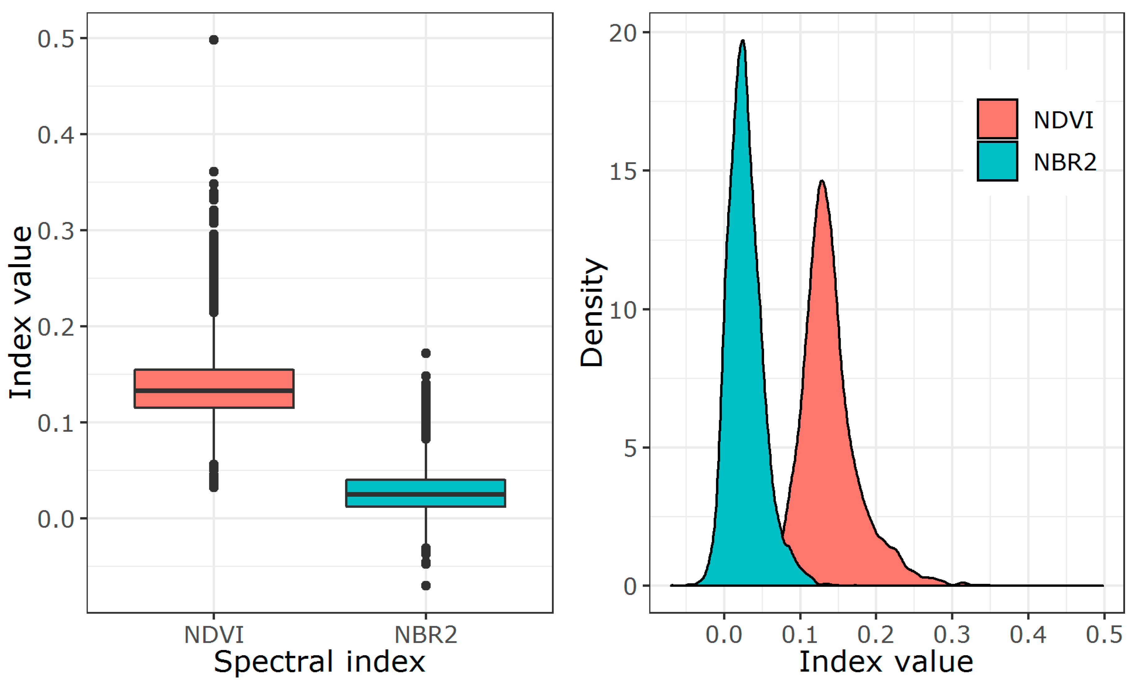
Bare soil composites were produced for an extent covering most of the European countries, situated between longitude −12 and 34 degrees, and latitude of 33 and 73 degrees. The algorithm Geospatial Soil Sensing System (GEOS3 [18]), developed within the Google Earth Engine [23], was used to generate the multispectral bare soil composites and the soil exposure frequencies from the collections of 30-m-resolution Landsat images from 1982 to 2018. The GEOS3 was slightly modified to adapt to several Landsat satellites with variable spectral characteristics but considering that the multispectral bands are positioned in equivalent spectral regions and their small differences do not affect the bare soil composites (

Table A1. Harmonization of the specific band numbers to common spectral names.

Common Name 1	Landsat 4 TM 2	Landsat 5 TM 3	Landsat 7 ETM+ 4	Landsat 8 OLI 5
Blue	1 (450–520 nm)	1 (450–520 nm)	1 (450–520 nm)	2 (452–512 nm)
Green	2 (520–600 nm)	2 (520–600 nm)	2 (520–600 nm)	3 (533–590 nm)
Red	3 (630–690 nm)	3 (630–690 nm)	3 (630–690 nm)	4 (636–673 nm)
NIR	4 (770–900 nm)	4 (770–900 nm)	4 (770–900 nm)	5 (851–879 nm)
SWIR1	5 (1550–1750 nm)	5 (1550–1750 nm)	5 (1550–1750 nm)	6 (1566–1651 nm)
SWIR2	7 (2080–2350 nm)	7 (2080–2350 nm)	7 (2080–2350 nm)	7 (2107–2294 nm)

¹ NIR: Near infrared; SWIR1: Shortwave infrared 1; SWIR2: Shortwave infrared 2. ² Landsat 4 Thematic Mapper (TM). ³ Landsat 5 Thematic Mapper (TM) sensor. ⁴ Landsat 7 Enhanced Thematic Mapper (ETM+) sensor. ⁵ Landsat 8 Operational Land Imager (OLI) sensor.

from Appendix A). GEOS3 is a data-mining algorithm that extracts soil features from the collection of historical images and aggregates the spatially bare soil fragments into a synthetic soil image (SYSI). The SYSI is the reflectance image of the bare soil composite, while the frequency of soil exposure is denominated as soil frequency (SF). SF is determined by the proportion of a given pixel location was identified as bare soil to the total number of pixel occurrences from the time interval of the collection. To identify bare soil pixels from single satellite images, a set of identification rules were used. They were based on spectral indices coupled with quality assessment bands, which removed cloud, cloud shadow, inland water, snow, photosynthetic vegetation and non-photosynthetic vegetation (crop residues). In this study, a pixel was flagged soil when it had the Normalized Difference Vegetation Index (NDVI, Equation (1)) values falling between the range of −0.05 and 0.30 (masking out green vegetation), and Normalized Burn Ration 2 index (NBR2, Equation (2)) values between the range of −0.15 and 0.15 (masking out crop residues). These thresholds were defined based on histogram and density plot analysis calculated from the LUCAS spectral measurements (Figure A1 from Appendix A). The flagged soil pixels were used to select each reflectance band on each acquisition time. Then the bare soil composite was composed by aggregating the multitemporal bare soil pixels by their median value. More detailed information about GEOS3, the spectral indices and sensitivity analysis of spectral indices thresholds are described in [18] or elsewhere [13,24,25,26].

$$\mathrm{NDVI}=\frac{\mathrm{NIR}-\mathrm{Red}}{\mathrm{NIR}+\mathrm{Red}}$$

(1)

$$\mathrm{NBR}2=\frac{\mathrm{SWIR}1-\mathrm{SWIR}2}{\mathrm{SWIR}1+\mathrm{SWIR}2}$$

(2)

where red (~630–690 nm), near infrared (NIR: ~760–900 nm), shortwave infrared 1 (SWIR1: ~1550–1750 nm) and shortwave infrared 2 (SWIR2: ~2080–2350 nm) are the harmonized spectral bands from Landsat 4 Thematic Mapper (L4 TM), Landsat 5 Thematic Mapper (L5 TM), Landsat 7 Enhanced Thematic Mapper Plus (L7 ETM+), and Landsat 8 Operational Land Imager (L8 OLI), respectively.

The bare soil composites (SYSIs) were produced using a harmonized and merged collection of surface reflectance images from the L4 TM (available images from 1982 to 1993), L5 TM (available images from 1984 to 2012), L7 ETM+ (available images from 1999 to present), and L8 OLI (available images from 2013 to present) available in Google Earth Engine datasets catalog [27,28,29]. Surface reflectance bands of each sensor were harmonized to a common band name that represented the same spectral range between the sensors (Table A1 from Appendix A). Although the relative spectral responses of instruments are slightly different and may cause effects on a time-series analysis [30], no significant effects were identified after merging the Landsat collections for aggregating SYSI over time. Some studies have also used this merging approach for increasing the availability of surface reflectance images, e.g., in [25,31], and consequently, improving the bare soil representation.

2.2. Reflectance Evaluation and Soil Dataset

To test the influence of temporal time frame considered for the calculation of the bare soil composite, two SYSIs were produced considering two different collections. The first SYSI was produced using a temporal subset from the full Landsat archive defined by 3 years before and after the LUCAS field survey of 2009 (2006–2012), which was called framed SYSI. The second SYSI was generated considering the full-time interval (1982–2018), being called full SYSI. We have generated the framed SYSI to check if significant changes would become evident when comparing its performance to the full SYSI. The two SYSI were compared using the correlation analysis with the reference topsoil spectra determined in laboratory, as well as by the performance after prediction. For evaluating the consistency of both SYSIs by the correlation analysis, we resampled the LUCAS spectra to the mean multispectral response of the four Landsat sensors and used the Spearman rank correlation analysis [32]. We used rank correlation analysis because we compared two domains (satellite and laboratory) that have different sensor and measurement characteristics, which interfere with the spectral response of soils. Therefore, this method was used to minimize the domain discrepancies and check if the rank of a sample from the first domain (laboratory) correspond to the rank of the same sample in the second domain (satellite). Despite the differences on the signal to noise ratio, the soil conditions and the temporal variability of satellite images when comparing laboratory and remote sensing data, the correlation coefficient gives an opportunity to understand if the patterns displayed in SYSI are linked to the soil reflectance, which considers in this case the laboratory measurements as the reference of the soil spectral response. For correlation analysis and prediction models, image data was sampled by intersecting the LUCAS coordinates with the SYSI bands.

Absorbance spectra and attributes data from the topsoil samples (0–20 cm) of the EU LUCAS database surveyed in 2009 were used in this study [33]. Approximately 20,000 topsoil samples were collected in 25 EU member states (EU-27 except Bulgaria and Romania). The soil sampling was undertaken within the frame of the Land-Use/Land-Cover Area Frame Survey, which represents one million points distributed in a grid of 2 × 2 km. The sample collected at each location followed a composite sampling strategy which comprised five topsoil (0–20 cm) subsamples that were mixed to form a single composite sample. The first subsample was taken at the coordinate point of the pre-established LUCAS point, whereas the remaining four are taken 2 m from the central one following the cardinal directions (North, East, South and West). Vegetation residues, grass, and litter, if present, were removed from the surface before sampling and from the composite sample. Soil samples have been analyzed for basic soil properties, including particle size distribution (soil texture), pH, organic carbon, carbonates, nitrogen, phosphorus, potassium, cation exchange capacity (CEC) and absorbance spectra, which was determined in the full continuous spectrum from 400 to 2500 nm and spectral resolution of 2 nm [33].

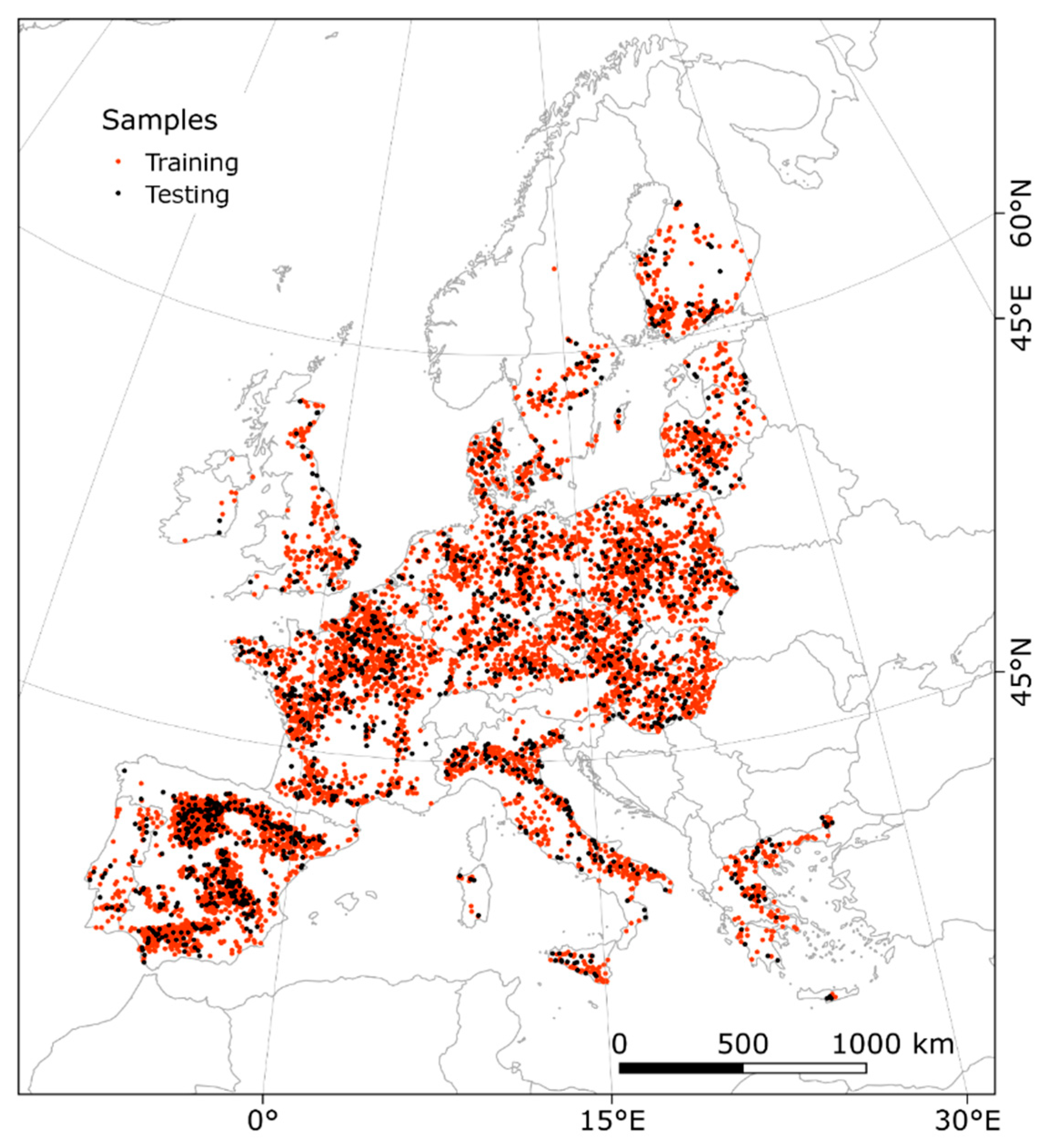
In this study, only samples from the main land cover type of croplands (category B) were selected from the 20,000 samples because most of the bare soils come from croplands, thus they have a more homogenized soil layer on the surface due to tillage operations. In the end, only 7142 samples were used from the original LUCAS dataset (Figure A2 in Appendix A). As the LUCAS spectral data are delivered in absorbance (A), we transformed the spectra to reflectance (R) by R = 1/10^A in order to correspond to the reflectance data of SYSIs. Besides the correlation analysis, the reflectance of LUCAS was also used to calibrate two reference models for comparing the prediction performance. For the first reference model, the LUCAS reflectance spectra (from 400 to 2500 nm) without any preprocessing method were transformed by principal component analysis (PCA) to reduce the spectral dimensionality, where the first five components that had a cumulative variance of more than 99% were submitted to model calibration. For the second reference model, the LUCAS reflectance spectra were resampled to the Landsat multispectral bands using the relative spectral responses of the four Landsat sensors [34], which were averaged to a single multispectral dataset for model calibration and correlation analysis.

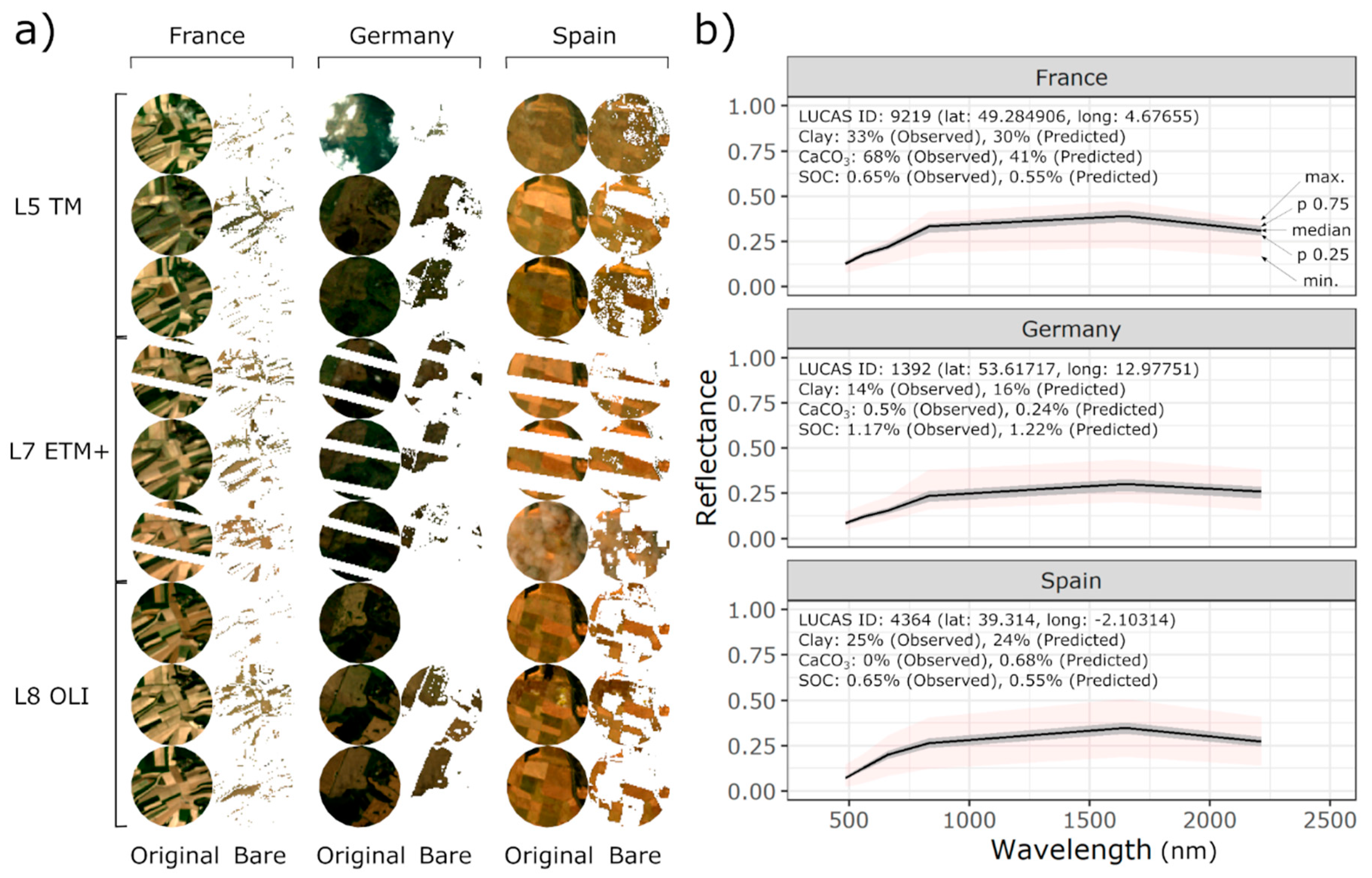
We also assessed the median reflectance generated from the full SYSI by inspecting its reflectance dispersion when the topsoil was identified as bare by GEOS3. Three random sites from France, Germany and Spain that were available in the EU LUCAS soil dataset (LUCAS IDS 9219, 1392, and 4364, respectively) were used for comparing subset images of the original true color composition and their respective bare soil masks. In this visualization step, three random scenes identified as bare in the L5 TM, L7 ETM + and L8 OLI collections were buffered by 1 km around the LUCAS geographical coordinate in order to visually compare the bare soil masked by GEOS3. At the same sites, the minimum, median, maximum and 0.25 and 0.75 percentiles of the reflectance were collected, making possible the evaluation of the soil reflectance dispersion. Site characteristics were also provided together with the spectral response to complement the SYSI reflectance evaluation.

2.3. Prediction Models of Soil Properties

Clay, sand, soil organic carbon (SOC), calcium carbonate (CaCO₃), pH determined in water (pH H₂O), and cation exchange capacity (CEC) data were selected to make prediction models. For this, we randomly split the dataset into training (80%) and test sets (20%). The prediction models were calibrated based either on the reflectance from the framed or the full SYSI, using the reflectance bands as predictors: blue (~450–520 nm), green (~520–600 nm), red (~630–690 nm), NIR (~760–900 nm), SWIR1 (~1550–1750 nm) and SWIR2 (~2080–2350 nm). Quantile regression from the gradient boosting trees (GBT) of scikit-learn Python library was used as the machine learning algorithm for calibrating prediction models [35]. Model tuning was performed using 10-fold cross-validation for the 0.50 percentile (median) of the training set trying different combinations of hyperparameters submitted to a grid search [36,37]. Learning rate was optimized from the set of 0.10, 0.15 and 0.20 units in order to control the magnitude of learning with the increasing number of trees. The number of estimators tested were 100, 250 and 500 trees to control the maximum number of trees for learning. These hyperparameters impact the forest used to ensemble the estimates. The maximum depth was tested in the set of respectively 5, 8 and 10 layers. The minimum samples at each split were optimized in the set of respectively 50, 100 and 200 samples. The minimum samples of each leaf were tested in the set of 5, 10, 20 samples. The maximum features used in each individual tree split was optimized in the set of 2, 4 and 6 predictors (6 is equals to the maximum number of predictors, i.e., the reflectance bands). These latter hyperparameters control individual trees in the GBT algorithm and are used to prevent specific learning of samples and reduce overfitting [38], making more robust and generalization models for spatially predicting the full geographical area. The best estimator was defined by the minimum root mean square error (RMSE, Equation (3)) from the 10-fold cross-validation of the training set, and the final hyperparameters are presented in

Table A2. Hyperparameters of the best regressions from gradient boosting trees, defined by 10-fold cross-validation of the training set (80%).

Soil Attribute 1	Reflectance Source 2	Seed	LR 3	NE 4	MF 5	MD 6	MSS 7	MSL 8
Clay	Original	1993	0.10	500	1	10	50	20
	Resampled	1993	0.20	500	6	10	50	10
	Framed SYSI	1993	0.10	250	6	5	100	20
	Full SYSI	1993	0.15	500	4	8	200	20
Sand	Original	1993	0.10	250	5	8	50	10
	Resampled	1993	0.10	500	4	10	50	20
	Framed SYSI	1993	0.10	250	4	10	100	5
	Full SYSI	1993	0.15	500	2	10	50	10
SOC	Original	1993	0.10	100	1	10	200	5
	Resampled	1993	0.10	500	6	5	50	20
	Framed SYSI	1993	0.10	100	2	5	100	20
	Full SYSI	1993	0.10	100	4	8	50	20
CaCO3	Original	1993	0.10	100	1	5	100	20
	Resampled	1993	0.20	500	2	8	50	20
	Framed SYSI	1993	0.10	100	4	8	100	20
	Full SYSI	1993	0.10	100	4	10	200	5
PH H2O	Original	1993	0.10	100	1	10	50	10
	Resampled	1993	0.10	500	6	8	50	20
	Framed SYSI	1993	0.15	250	4	10	100	20
	Full SYSI	1993	0.15	250	4	8	200	20
CEC	Original	1193	0.10	250	1	10	50	20
	Resampled	1993	0.10	500	6	10	50	20
	Framed SYSI	1993	0.10	100	4	8	200	20
	Full SYSI	1993	0.10	500	4	8	200	20

¹ Soil attributes: Soil organic carbon (SOC), calcium carbonate (CaCO₃), pH determined in water solution (pH H₂O), and cation exchange capacity (CEC). ² Synthetic soil image (SYSI). Original and Resampled terms refer to the LUCAS absorbance spectra (450 to 2500 nm) used as reference prediction models, where the original was converted to reflectance and reduced by principal component analysis, and the resampled was converted to reflectance and resampled to the Landsat multispectral bands. Hyperparameters of gradient boosting trees from scikit-learn Python library: ³ learning_rate (LR); ⁴ n_estimators (NE); ⁵ max_features (MF); ⁶ max_depth (MD); ⁷ min_samples_split (MSS); ⁸ min_samples_leaf (MSL).

of Appendix A.

Before the model calibration, the soil attributes values were logit-transformed to constrain the predicted range to a defined maximum and minimum limit [39], with the predictions back transformed for generating the maps and assessing the performance. To assess the model performance, the following parameters were calculated from the test set: the RMSE (Equation (3)) was measured to evaluate the model’s inaccuracy; the coefficient of determination (R², Equation (4)) was calculated to evaluate the explained variance of models; and the ratio of performance to interquartile range (RPIQ, Equation (5)) was estimated to assess the consistency between the predicted values and the testing dataset variability [40].

$$\mathrm{RMSE}=\sqrt{\frac{{{\displaystyle \sum }}_{i=1}^n{\left(\widehat{y_i}-y_i\right)}^2}{n}}$$

(3)

$${\mathrm{R}}^2=1-\frac{{{\displaystyle \sum }}_{i=1}^n{\left(\widehat{y_i}-y_i\right)}^2}{{{\displaystyle \sum }}_{i=1}^n{\left(y_i-\overline{y}\right)}^2}$$

(4)

$$\mathrm{RPIQ}=\frac{{\mathrm{IQR}}_y}{{\mathrm{RMSE}}_{\widehat{y}}}$$

(5)

where $y$ is the vector of measured values, $\widehat{y}$ is the vector of predicted values, $\overline{y}$ is the mean of vector $y$, and IQR is the interquartile range defined by the differences of 75th and 25th percentiles.

2.4. Spatial Prediction and Uncertainty

For the development of maps of soil properties, the best spectral model derived from the framed or full SYSI was selected from the evaluation metrics and employed for predicting cropland soils across the European extent. In this step, we used the CORINE land-cover map of 2012 (version 20) to restrict our predictions, considering in this case, the grouping of ‘non-irrigated arable land’, ‘permanently irrigated land’, ‘rice fields’, and ‘annual crops associated with permanent crops’ classes [41]. Soil attribute maps of the median estimate (0.50 percentile) and 90% prediction interval defined by 0.05 and 0.95 percentiles were produced. Uncertainty at the pixel level was defined as the ratio between the 90% prediction interval to the median estimate, which was then converted to the percent scale. Thus, as the uncertainty is standardized to the median estimate, we can compare both the spatial patterns and the differences between the uncertainty maps. Additionally, to visually asses the regional variability of the predicted clay map, four different locations were selected based on the spatial variability of soils and previous works developed at the same sites [13,42,43,44,45].

The predictions were made for separated tiles of 1 × 1 degree using multi-core processing. Overviews (levels 2 [pixel resolution of 60 m], 4 [pixel resolution of 120 m], and 8 [pixel resolution of 240 m]) and virtual raster were used for mosaicking the tiles and displaying the original 30-m-resolution maps over the European extent. The statistical analysis, machine learning and map visualizations were performed using free and open source software: Python 3.6 [46], GDAL [47], R 3.4 [48], and Quantum GIS 3.4 [49].

3. Results

3.1. Bare Soil Composites

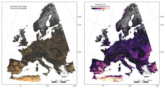
The full SYSI produced across the croplands within the European extent reveals different patterns represented by the true color composition (Figure 1a). Soil surfaces in Southern Europe are brighter than the other regions, probably because of the semi-arid conditions relatively dominated by iron oxides, sand and clays [44]. Conversely, the Eastern part of the map have a darker shade, which could be linked to soil types with dark surface horizons, such Chernozems and Phaeozems [50]. The frequency of soil exposure (Figure 1b), which represents how many times a site was identified as bare during the time interval of the multitemporal collection, also gives an opportunity to understand the degree of soil disturbance, which can be linked to natural factors, such as the type of land cover, or even human-induced factors, such as the disturbances caused by tillage operations. The remaining white areas in both panels are due to the absence of bare surface information that was masked by a cropland reference map of 2012. Despite the fact that framed SYSI had, in general, similar patterns as the full SYSI, framed SYSI yielded a lower proportion of bare soils and is not presented in this section. However, the statistical evaluation of both SYSIs is described below.

3.2. Soil Dataset and Reflectance Evaluation

The summary statistics of the soil attributes used in this study are demonstrated in

Table 1. Descriptive statistics of soil samples subset from the Land-Use/Land-Cover Area Frame Survey (LUCAS) topsoil database (n = 7142).

Variable 1	Min. 2	Mean	SD 3	Median	IQR 4	Max. 5
Soil Attributes
Clay (%)	1.00	21.94	12.58	21.00	16.00	79.00
Sand (%)	1.00	36.02	25.12	31.00	41.00	97.00
SOC (%)	0.00	1.68	1.56	1.38	0.94	43.84
CaCO3 (%)	0.00	9.01	15.91	0.30	11.30	88.20
pH H2O	3.55	7.05	1.01	7.33	1.58	8.93
CEC (cmolc kg−1)	0.00	15.30	9.40	13.80	11.30	188.10
Resampled reflectance from laboratory
Blue	0.03	0.15	0.05	0.14	0.05	0.50
Green	0.04	0.21	0.06	0.20	0.08	0.61
Red	0.05	0.27	0.07	0.27	0.10	0.67
NIR	0.10	0.36	0.08	0.36	0.10	0.75
SWIR1	0.17	0.48	0.08	0.48	0.10	0.81
SWIR2	0.15	0.45	0.07	0.45	0.09	0.74
Reflectance from framed SYSI 6
Blue	0.03	0.08	0.02	0.08	0.02	0.15
Green	0.04	0.12	0.03	0.12	0.03	0.23
Red	0.03	0.15	0.04	0.15	0.05	0.33
NIR	0.05	0.23	0.05	0.23	0.07	0.43
SWIR1	0.02	0.30	0.06	0.29	0.08	0.54
SWIR2	0.02	0.24	0.05	0.24	0.07	0.43
Reflectance from full SYSI
Blue	0.04	0.08	0.02	0.08	0.02	0.14
Green	0.04	0.12	0.03	0.12	0.03	0.22
Red	0.04	0.15	0.04	0.15	0.05	0.33
NIR	0.05	0.23	0.05	0.23	0.06	0.43
SWIR1	0.03	0.29	0.06	0.29	0.08	0.53
SWIR2	0.03	0.24	0.05	0.24	0.06	0.42

¹ Soil attributes: soil organic carbon (SOC), calcium carbonate (CaCO₃), pH determined in water solution (pH H₂O), cation exchange capacity (CEC). Reflectance bands: blue (~450–520 nm), green (~520–600 nm), red (~630–690 nm), near infrared (NIR: ~760–900 nm), shortwave infrared 1 (SWIR1: ~1550–1750 nm) and shortwave infrared 2 (SWIR2: ~2080–2350 nm). ² Minimum value. ³ Standard deviation (SD). ⁴ Interquartile range (IQR). ⁵ Maximum value. ⁶ Synthetic soil image (SYSI).

. Clay values ranged from 1% to 79%, with a mean value of 22% and standard deviation (SD) of almost 13%, indicating a higher predominance of medium textured soils in the dataset (mean and SD sand values: 36% and 25%, respectively). SOC values were variable and ranged from 0 to 43.84%, with a low mean value of 1.68% and SD of 1.56%, probably because of the absence of higher SOC content samples that are common in other land cover classes, such as grasslands and forests. Calcium carbonate content (CaCO₃) varied between 0% and 88%, with a mean value of 9%, while pH determined in water had a mean value close to 7 (SD of 1.01). The mean value of cation exchange capacity (CEC) was estimated in 15.30 cmol_c kg⁻¹, with a SD of 9.40 cmol_c kg⁻¹.

Table 1 also shows the summary statistics of the different reflectance sources and highlights the discrepancies between LUCAS resampled reflectance with the median reflectance of framed and full SYSI. Laboratory spectral measurements resampled to Landsat multispectral range had a higher reflectance intensity for all the bands, with the mean value being in general twice the value of the reflectance of bare soil composites. The contrasting intensities can be linked to different measurement and soil conditions of the two acquisition levels, where in the laboratory the illumination and geometrical factors, and sample conditions, are controlled. Also, there could be a mixing of patterns in the field-of-view at the satellite level that reduces the overall reflectance. The field-of-view and the signal-to-noise ratio of sensors is another factor that is very contrasting between laboratory and spaceborne sensors, even for field reflectance measurements.

Simple correlations between the laboratory and bare soil composite bands were moderate with coefficients varying from 0.49 to 0.66 (

Table 2. Spearman correlation between laboratory resampled reflectance and synthetic soil images.

Correlation 1	Blue	Green	Red	NIR	SWIR1	SWIR2
Resampled~Framed SYSI	0.60	0.62	0.62	0.60	0.59	0.49
Resampled~Full SYSI	0.63	0.66	0.66	0.65	0.63	0.53
Framed SYSI~Full SYSI	0.90	0.93	0.94	0.93	0.94	0.93

¹ All correlations are significant at p < 0.05. Reflectance bands: blue (~450–520 nm), green (~520–600 nm), red (~630–690 nm), near infrared (NIR: ~760–900 nm), shortwave infrared 1 (SWIR1: ~1550–1750 nm) and shortwave infrared 2 (SWIR2: ~2080–2350 nm).

). Although the reflectance values have different amplitude, as demonstrated in Table 1, we can see that the correlation between both the sources still exists. Framed SYSI had a slightly lower correlation with the laboratory reflectance than the full SYSI. For the framed SYSI, the correlation coefficients ranged from 0.49 to 0.62, while for the full SYSI they ranged from 0.53 to 0.66. This result gives a first idea that framing the generation of a bare soil composite to the soil sample survey time might not improve the reflectance accuracy when using the GEOS3 methodology, which is based on the median reflectance of the bare soil pixels. Here, an assumption is that the longer time frame of the full SYSI provides a more stable median reflectance that is less affected by dynamic effects of the bare soils. Additionally, there could be a limitation of generating a bare soil composite using a shorter historical collection, which would retrieve only a few bare soil exposures along the time series that would not be sufficient for estimating a robust median value closer to ideal bare soil conditions (e.g., dried, vegetation-free). Therefore, we selected the full SYSI as the best representative of the bare topsoil reflectance for the further analyses.

Another way of assessing the median reflectance generated from the full SYSI was by inspecting the dispersion of the reflectance when the surface was identified as bare by GEOS3 (Figure 2). Different sampling sites from France, Germany and Spain from the LUCAS dataset were used in this additional evaluation. The land use and the geographical characteristics of the sites affects the amount of bare soil that can be extracted by GEOS3 (Figure 2a), regardless the Landsat sensor. For example, the selected site in Spain (LUCAS ID 4364) provided a higher proportion of bare soils than the sites from Germany and France, which can be probably linked to the dryer climate and also to a higher intensive land use. Despite the occurrence of extreme values as demonstrated by the minimum and maximum values in the spectral plots (Figure 2b), we can observe that the median statistics provide a reasonable estimate of bare soil reflectance, with a lower dispersion defined by the interquartile range (0.75 and 0.25 percentiles, represented by the gray shadow). The site in France has the highest median intensity, with a higher decrease of reflectance between 2000 and 2500 nm, which can be linked to its higher clay and CaCO₃ contents. Overall, full SYSI provided a good estimate for the bare soil reflectance and was used in the further steps of the study for predicting cropland soil attributes across the European extent.

3.3. Prediction Models

Table 3. Performance of prediction models of soil properties (n = 7142) using reflectance data.

Attribute 1	Reflectance Data 2	3 R2	RMSE 4	RPIQ 5	R2	RMSE	RPIQ
		Training Set (80%)			Testing Set (20%)
Clay (%)	Original	0.80	5.57	2.87	0.58	8.35	2.04
	Resampled	0.78	5.80	2.76	0.49	9.18	1.85
	Framed SYSI	0.53	8.58	1.87	0.36	10.28	1.65
	Full SYSI	0.67	7.20	2.22	0.44	9.59	1.77
Sand (%)	Original	0.66	14.57	2.81	0.42	19.26	2.23
	Resampled	0.72	13.27	3.01	0.37	20.07	2.14
	Framed SYSI	0.56	16.54	2.42	0.22	22.39	1.92
	Full SYSI	0.68	14.10	2.84	0.25	21.93	1.96
SOC (%)	Original	0.35	1.09	0.86	0.24	1.52	0.58
	Resampled	0.25	1.31	0.72	0.13	1.62	0.54
	Framed SYSI	0.10	1.44	0.66	0.04	1.69	0.52
	Full SYSI	0.16	1.39	0.68	0.06	1.68	0.52
CaCO3 (%)	Original	0.59	10.97	1.70	0.54	11.89	1.82
	Resampled	0.76	8.48	2.30	0.47	12.70	1.70
	Framed SYSI	0.47	12.56	1.55	0.31	14.50	1.49
	Full SYSI	0.51	12.18	1.60	0.36	13.99	1.54
pH H2O	Original	0.62	0.63	2.48	0.39	0.80	2.05
	Resampled	0.62	0.62	2.52	0.31	0.85	1.93
	Framed SYSI	0.46	0.74	2.10	0.14	0.94	1.73
	Full SYSI	0.45	0.75	2.08	0.21	0.90	1.80
CEC (cmolc kg−1)	Original	0.70	4.38	2.32	0.38	7.66	1.46
	Resampled	0.66	5.35	2.11	0.32	8.02	1.39
	Framed SYSI	0.39	7.16	1.58	0.22	8.60	1.30
	Full SYSI	0.54	6.24	1.81	0.28	8.25	1.35

¹ Soil attributes: Soil organic carbon (SOC), calcium carbonate (CaCO₃), pH determined in water solution (pH H₂O), and cation exchange capacity (CEC). ² Synthetic Soil Image (SYSI); Original and Resampled terms refer to the LUCAS absorbance spectra (450 to 2500 nm) used as reference prediction models, where the original was converted to reflectance and reduced by principal component analysis, and the resampled was converted to reflectance and resampled to the Landsat multispectral bands. ³ Coefficient of determination (R²). ⁴ Root mean squared error (RMSE). ⁵ Ratio of performance to interquartile range (RPIQ).

shows the performance of the gradient boosting tree regressions for each of the six soil attributes using four different reflectance data. The LUCAS original and resampled reflectance datasets deliver the best performances for almost all the attributes in both training and testing sets, confirming its superior composition for calibrating spectral prediction models. However, the soil organic carbon was unable to be predicted (R² < 0.35 and RPIQ < 1.5 in training and testing sets) even considering the LUCAS laboratory data. In particular, texture attributes and calcium carbonate content had the best calibration and testing performance for all datasets (R² > 0.35 and RPIQ > 1.5), except for framed SYSI. Additionally, we can identify from the testing results that there is an inferior performance for both SYSI models compared to the reference models of laboratory data. This result can be associated to measurement characteristics and soil surface conditions of satellite acquisition level, and possibly to the effect of integrating pixel values to point coordinates (support change). Nonetheless, the results demonstrate that the full SYSI can still be used as a covariate for building prediction models based on its median reflectance values. Another point that is worth mentioning is that framing the SYSI to soil survey period does not improve the prediction performance, suggesting that the full SYSI have the most reliable estimate of the median topsoil reflectance after using a denser historical collection (37 years).

3.4. Spatial Predictions and Uncertainty

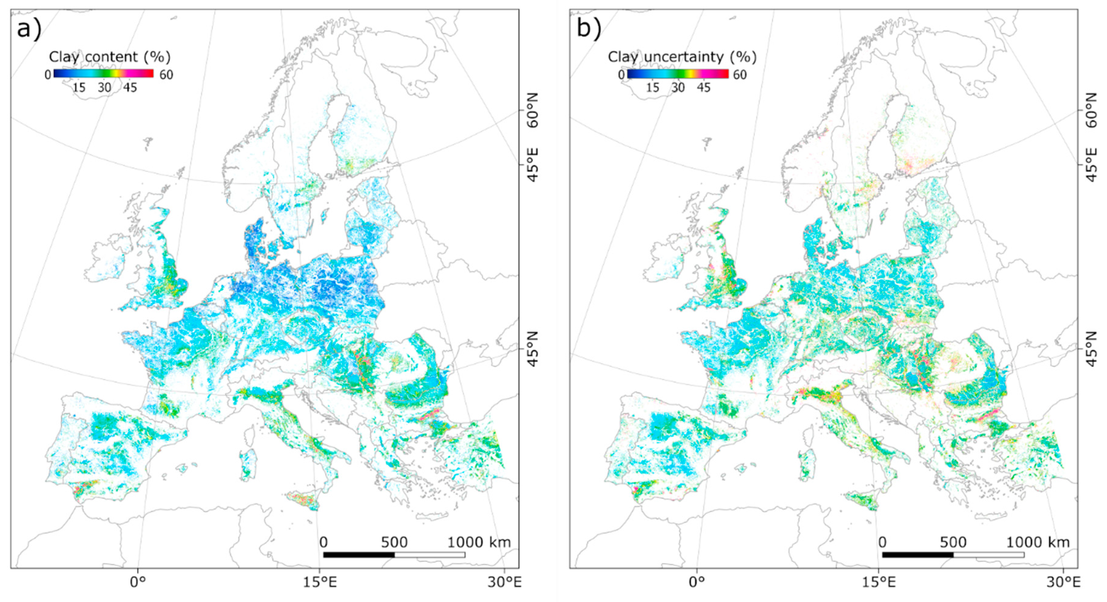
The predicted clay content of croplands across the European geographical extent (using the full SYSI) showed the predominance of soils with low to medium clay content (Figure 3a). Soils with low clay estimates prevail from the central of Western to Eastern Europe. Conversely, soils rich in clay are more evident in some regions of the United Kingdom, Spain, Italy and the Southeastern of Europe. The uncertainty of predictions (Figure 3b), estimated as the 90% prediction interval standardized to the median estimate, reveals that croplands with higher estimates of clay can have in some cases, a high uncertainty, i.e., there is a high variation around the predicted median value. This observation coincides with the croplands in the North of Italy and in the United Kingdom.

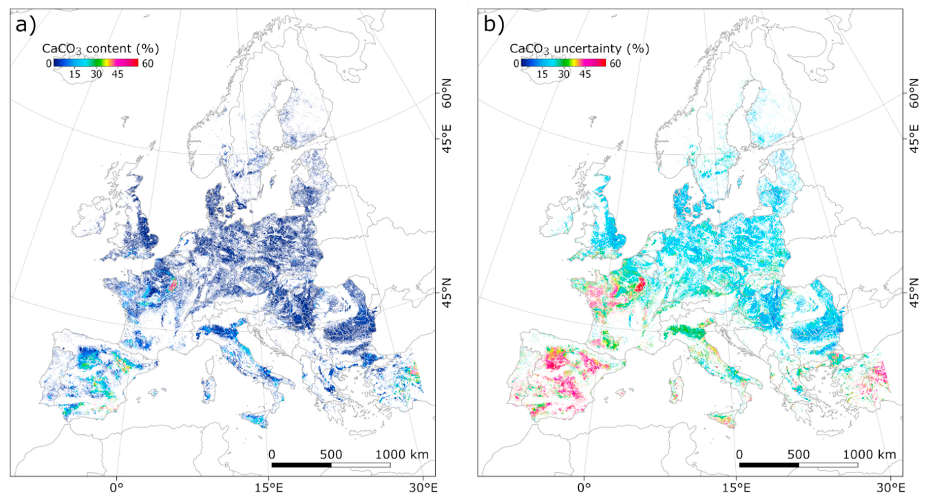
Calcium carbonate content was also estimated across the croplands within the European extent using the full SYSI (Figure 4a). In this map, lower carbonate contents predominate across the European extent, which is possibly related to low abundance (mean and median values) already expressed in the samples from the LUCAS dataset (Table 1). The Champagne region in France and some soils of Spain had the highest estimates of CaCO₃, although the uncertainty was also considered moderately high (Figure 4b). Other sites in Italy, Greece and the Mediterranean region also had significant estimates of CaCO₃ as displayed by light blue shades in Figure 4a. These mapped areas coincide with calcium-rich lithology that forms CaCO₃ rich soils, suggesting that multispectral reflectance from bare soil composites can be relevant for mapping this soil attribute over croplands.

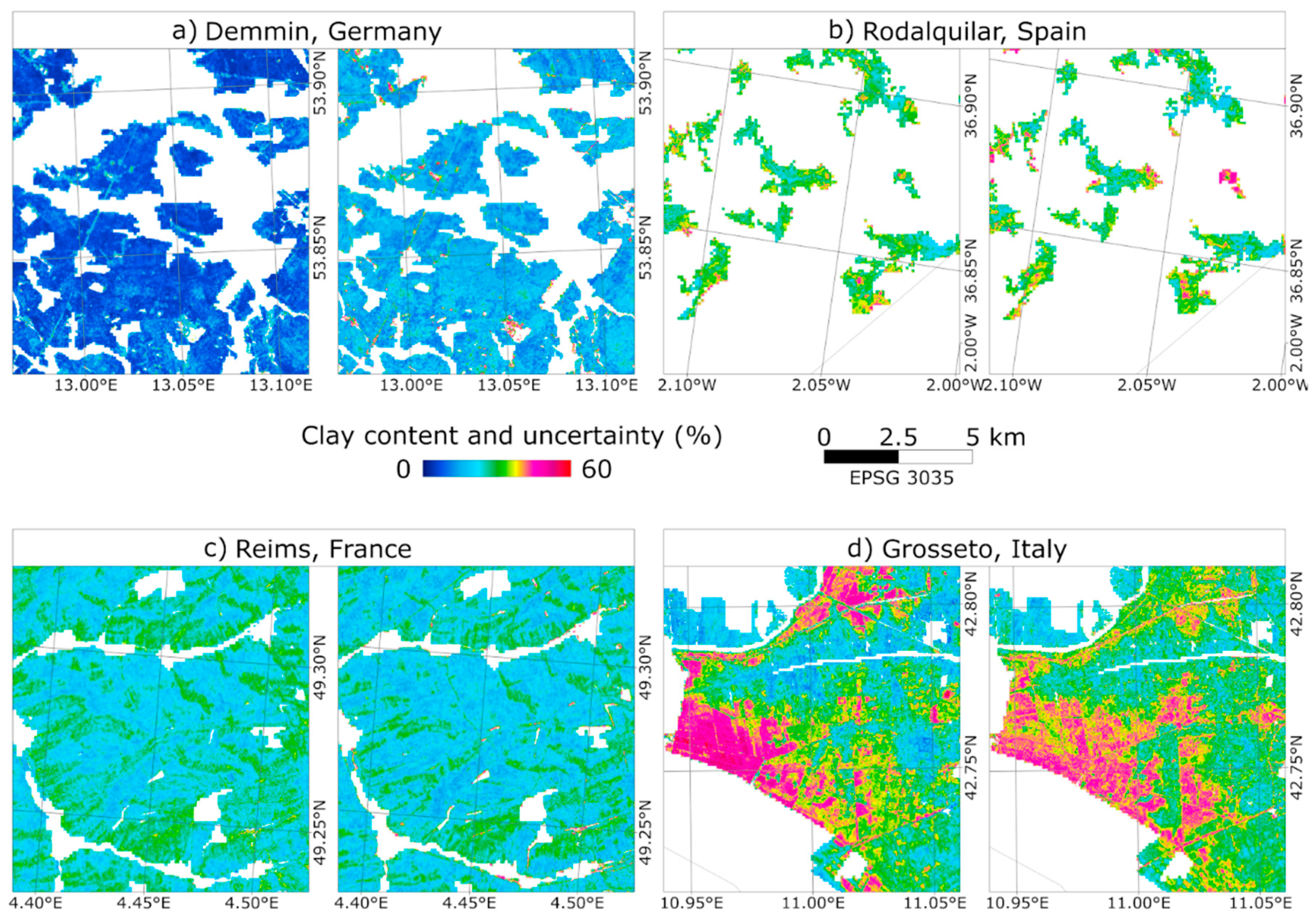
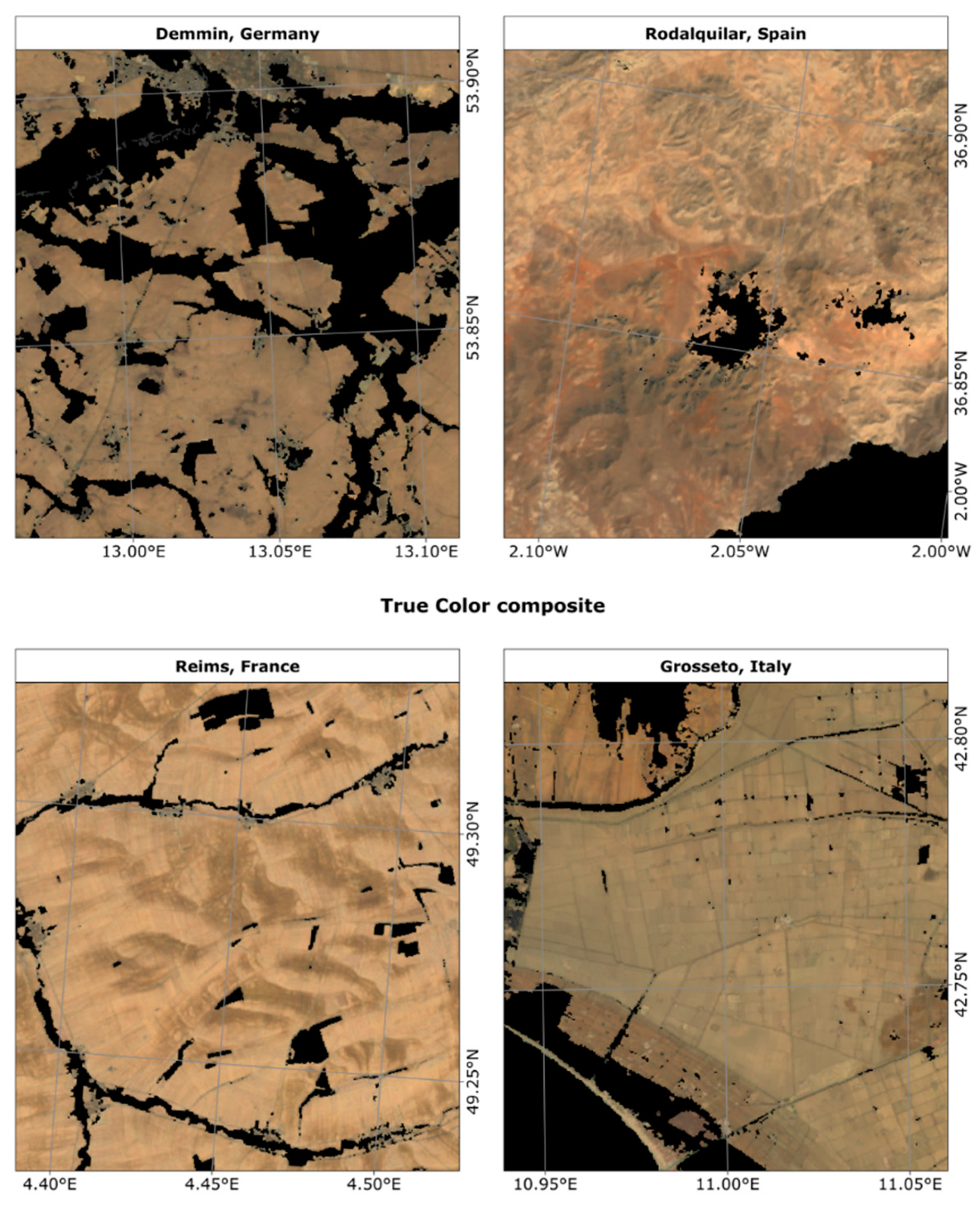
The clay maps were also checked at the regional level by inspecting the predictions produced from the full SYSI (Figure 5). Four different regions across the European extent were selected to check the spatial variability of clay, which included sites from Germany (Figure 5a), Spain (Figure 5b), France (Figure 5c), and Italy (Figure 5d). The regional maps seem to aid the recognition of the local variability of clay content, which can be important for a more efficient management of croplands, for example. The spatial patterns in these images can be linked to lithological variability, which affects the soil texture. In general, the comparison of these regional mapping fits well with previous published results for these regions [13,42,43,44,45]. The true color composites (full SYSI) for the same sites of Figure 5 are provided in Figure A3 in Appendix A.

4. Discussion

Framing the SYSI generation to the soil observation survey was a more reasonable approach for generating a bare soil composite, especially for predicting dynamic soil properties, such as SOC and chemical soil properties. However, the median reflectance estimated by the full SYSI had a higher correlation with the reference spectra collected in the laboratory, which resulted in more accurate predictions by machine learning. Some studies have already pointed out that denser collections of historical images increase the probability of retrieving more bare soils over a given area, which increases the mapped area and the quality of topsoil reflectance [16,18,31].

After employing the reflectance from bare soil composites to machine learning, the evaluation metrics revealed that CaCO₃ and clay attributes yielded the best prediction performances (Table 2). Many studies have demonstrated that clay and calcium carbonates have distinctive absorption characteristics in VIS-NIR-SWIR region [11,51,52] including albedo, shape, and absorption features, which could explain why these two soil attributes had the highest accuracies. In the bare soil composites, although specific absorption features are not depicted due to the lower resolution of multispectral data, the intensity and shape were influenced by soil constituents, in accordance with the findings of [53]. Furthermore, studies that compared different acquisition levels for predicting either clay or carbonate topsoil contents confirm that laboratory-based spectra give the best estimates, although field and aerial data can also be employed for depicting the spatial variability of clay and CaCO₃ [11,52].

In the work performed by [11], the effectiveness of continuum-removed absorption features for clay and CaCO₃ prediction from different hyperspectral acquisition levels was tested. The spectral consistency changes from laboratory to aerial sensors were also assessed in that study. Their results confirmed that simple models based on absorption features are efficient in predicting clay and CaCO₃ estimates regardless of the source [34]. Our results obtained from a multispectral approach confirmed that it is possible to map these two soil attributes using the bare soil reflectance and a large SSL as ground data for calibration. However, the prediction of soil attribute using multispectral reflectance relies on the total apparent reflectance value (albedo) rather than specific absorption features [53], which are usually employed in a specific group of soils that are measured by the same protocol (sample preparation, spectroradiometer, and lightening configuration).

Soil spectral libraries (employed in laboratory) have been extensively explored in soil spectroscopy and digital soil mapping and have become an alternative for traditional wet analysis for some specific attributes. Transferring multispectral or hyperspectral prediction models from laboratory to bare soil images seems to be challenging. The uncertainty is high because not only do the acquisition means hamper the predictions, but also the temporal and surface conditions degrade the signal of soils in satellite images [11,20,54]. Differences in reflectance intensities make difficulty for the transfer of a prediction model without standardizing the data, as the model’s coefficients of one level might yield biased estimates on the other. In addition, there are other aspects that pose limitations when integrating soil spectral libraries to multispectral bare soil composites. Since the soil spectral reflectance is determined by several soil properties that usually vary in space and time, the sampling design must consider the variability of soils in adequate scales, i.e., usually at the regional or local level. It is also important to take into consideration the temporal changes that can happen for some soil attributes, such as SOC, pH and soil elements. These characteristics can affect model calibration, resulting in poor validation performance and the generalization of predictions, similarly to what was found for SOC, pH and CEC in this study (Table 3). Furthermore, the change of support from pixels to coordinate points may also be assessed when integrating SSL to bare soil images. The optimal condition for integrating these data takes into account the pixel variability within a certain extent around the point coordinate, followed by the fitting of a spatial model to predict a value exactly at the point coordinate [1,55]. This approach could correct the differences between the point and pixel support but are still subjected to some additional definitions, such as the extent size around the point coordinate (number of pixels) and other spatial model parameters. Similarly, the subsampling design of soil samples at the coordinate points may also affect the integration, i.e., whether the point was comprised of a single instance (point support) or many composite samples (areal support). Thus, as these additional factors can impact the results derived from bare soil composites, they may be addressed in future works.

Nonetheless, there is still room for exploring the transferring approach using bare soil composites, mainly considering forthcoming hyperspectral images and more advanced machine learning frameworks [56,57]. Bare soil composites derived from hyperspectral imagers, either aerial or orbital, can be exploited in future investigations because they provide images with more spectral bands and higher spectral resolution, which can be associated to specific absorption features. This is the case of the current hyperspectral in orbit PRISMA (PRecursore IperSpettrale della Missione Applicativa [58]) and of the other upcoming hyperspectral imagers, such as the German EnMAP (Environmental Mapping and Analysis Program [59]). Other machine-learning frameworks and standardization methods can also be investigated on transferring prediction models from laboratory to satellite levels. This could be the case of convolution neural networks using the model transfer approach by fine tuning the models to the acquisition and/or spatial domains [20,54]. In the work performed by [20], the researches successfully transferred a clay prediction model calibrated from LUCAS laboratory spectral data to a hyperspectral aerial image covering a small region in Spain, reaching an R² of 0.60 and RMSE of 8.62% using convolutional neural networks.

5. Conclusions

This study supports the proposition that bare soil composites can be generated over the European extent for developing topsoil prediction models of clay and calcium carbonates of cropland soils. Our approach used the median reflectance of 37 years of Landsat imagery for reducing extreme estimates along the multitemporal survey. Further, prediction models were established using gradient boosting tree regressions coupled with a subset of the EU LUCAS soil dataset. We propose that this approach can be added to digital soil mapping seeking to improve the topsoil prediction of croplands at a regional or local level, since the topsoil of this land use is more homogeneous due to tillage practices. We also found that generating a bare soil composite displaced to the survey time of soil survey did not affect the prediction accuracy of relatively stable soil attributes, i.e., clay and calcium carbonates. In fact, a denser historical collection increases the chances of retrieving more exposed surfaces, which improves the representation of diverse soils.

References

- Ben-Dor, E.; Chabrillat, S.; Demattê, J.A.M.; Taylor, G.R.; Hill, J.; Whiting, M.L.; Sommer, S. Using Imaging Spectroscopy to study soil properties. Remote Sens. Environ. 2009, 113, S38–S55. [Google Scholar] [CrossRef]
- Summers, D.; Lewis, M.; Ostendorf, B.; Chittleborough, D. Visible near-infrared reflectance spectroscopy as a predictive indicator of soil properties. Ecol. Indic. 2011, 11, 123–131. [Google Scholar] [CrossRef]
- Viscarra Rossel, R.A.; Behrens, T.; Ben-Dor, E.; Brown, D.J.; Demattê, J.A.M.; Shepherd, K.D.; Shi, Z.; Stenberg, B.; Stevens, A.; Adamchuk, V.; et al. A global spectral library to characterize the world’s soil. Earth-Sci. Rev. 2016, 155, 198–230. [Google Scholar] [CrossRef] [Green Version]
- Nocita, M.; Stevens, A.; Toth, G.; Panagos, P.; van Wesemael, B.; Montanarella, L. Prediction of soil organic carbon content by diffuse reflectance spectroscopy using a local partial least square regression approach. Soil Biol. Biochem. 2014, 68, 337–347. [Google Scholar] [CrossRef]
- Gholizadeh, A.; Saberioon, M.; Carmon, N.; Boruvka, L.; Ben-Dor, E. Examining the Performance of PARACUDA-II Data-Mining Engine versus Selected Techniques to Model Soil Carbon from Reflectance Spectra. Remote Sens. 2018, 10, 1172. [Google Scholar] [CrossRef] [Green Version]
- Demattê, J.A.M.; Dotto, A.C.; Paiva, A.F.S.; Sato, M.V.; Dalmolin, R.S.D.; de Araújo, M.d.S.B.; da Silva, E.B.; Nanni, M.R.; ten Caten, A.; Noronha, N.C.; et al. The Brazilian Soil Spectral Library (BSSL): A general view, application and challenges. Geoderma 2019, 354, 113793. [Google Scholar]
- Ng, W.; Minasny, B.; Montazerolghaem, M.; Padarian, J.; Ferguson, R.; Bailey, S.; McBratney, A.B. Convolutional neural network for simultaneous prediction of several soil properties using visible/near-infrared, mid-infrared, and their combined spectra. Geoderma 2019, 352, 251–267. [Google Scholar] [CrossRef]
- Ramirez-Lopez, L.; Wadoux, A.M.J.-C.; Franceschini, M.H.D.; Terra, F.S.; Marques, K.P.P.; Sayão, V.M.; Demattê, J.A.M. Robust soil mapping at the farm scale with vis–NIR spectroscopy. Eur. J. Soil Sci. 2019, 70, 378–393. [Google Scholar] [CrossRef] [Green Version]
- Ben-Dor, E.; Ong, C.; Lau, I.C. Reflectance measurements of soils in the laboratory: Standards and protocols. Geoderma 2015, 245–246, 112–124. [Google Scholar] [CrossRef]
- Chabrillat, S.; Ben-Dor, E.; Cierniewski, J.; Gomez, C.; Schmid, T.; van Wesemael, B. Imaging Spectroscopy for Soil Mapping and Monitoring. Surv. Geophys. 2019, 40, 361–399. [Google Scholar] [CrossRef] [Green Version]
- Lagacherie, P.; Baret, F.; Feret, J.-B.; Madeira Netto, J.; Robbez-Masson, J.M. Estimation of soil clay and calcium carbonate using laboratory, field and airborne hyperspectral measurements. Remote Sens. Environ. 2008, 112, 825–835. [Google Scholar] [CrossRef]
- Diek, S.; Chabrillat, S.; Nocita, M.; Schaepman, M.E.; de Jong, R. Minimizing soil moisture variations in multi-temporal airborne imaging spectrometer data for digital soil mapping. Geoderma 2019, 337, 607–621. [Google Scholar] [CrossRef]
- Castaldi, F.; Chabrillat, S.; Don, A.; van Wesemael, B. Soil Organic Carbon Mapping Using LUCAS Topsoil Database and Sentinel-2 Data: An Approach to Reduce Soil Moisture and Crop Residue Effects. Remote Sens. 2019, 11, 2121. [Google Scholar] [CrossRef] [Green Version]
- Ustin, S.L.; Roberts, D.A.; Gamon, J.A.; Asner, G.P.; Green, R.O. Using Imaging Spectroscopy to Study Ecosystem Processes and Properties. Bioscience 2004, 54, 523–534. [Google Scholar] [CrossRef]
- Ben-Dor, E.; Granot, A.; Notesco, G. A simple apparatus to measure soil spectral information in the field under stable conditions. Geoderma 2017, 306, 73–80. [Google Scholar] [CrossRef]
- Diek, S.; Fornallaz, F.; Schaepman, M.E.; de Jong, R. Barest Pixel Composite for agricultural areas using landsat time series. Remote Sens. 2017, 9, 1245. [Google Scholar] [CrossRef] [Green Version]
- Rogge, D.; Bauer, A.; Zeidler, J.; Mueller, A.; Esch, T.; Heiden, U. Building an exposed soil composite processor (SCMaP) for mapping spatial and temporal characteristics of soils with Landsat imagery (1984–2014). Remote Sens. Environ. 2018, 205, 1–17. [Google Scholar] [CrossRef] [Green Version]
- Demattê, J.A.M.; Fongaro, C.T.; Rizzo, R.; Safanelli, J.L. Geospatial Soil Sensing System (GEOS3): A powerful data mining procedure to retrieve soil spectral reflectance from satellite images. Remote Sens. Environ. 2018, 212, 161–175. [Google Scholar] [CrossRef]
- Tao, C.; Wang, Y.; Cui, W.; Zou, B.; Zou, Z.; Tu, Y. A transferable spectroscopic diagnosis model for predicting arsenic contamination in soil. Sci. Total Environ. 2019, 669, 964–972. [Google Scholar] [CrossRef]
- Liu, L.; Ji, M.; Buchroithner, M. Transfer Learning for Soil Spectroscopy Based on Convolutional Neural Networks and Its Application in Soil Clay Content Mapping Using Hyperspectral Imagery. Sensors 2018, 18, 3169. [Google Scholar] [CrossRef] [Green Version]
- Andrew, A.; Fearn, T. Transfer by orthogonal projection: Making near-infrared calibrations robust to between-instrument variation. Chemom. Intell. Lab. Syst. 2004, 72, 51–56. [Google Scholar] [CrossRef]
- Feudale, R.N.; Woody, N.A.; Tan, H.; Myles, A.J.; Brown, S.D.; Ferré, J. Transfer of multivariate calibration models: A review. Chemom. Intell. Lab. Syst. 2002, 64, 181–192. [Google Scholar] [CrossRef]
- Gorelick, N.; Hancher, M.; Dixon, M.; Ilyushchenko, S.; Thau, D.; Moore, R. Google Earth Engine: Planetary-scale geospatial analysis for everyone. Remote Sens. Environ. 2017, 202, 18–27. [Google Scholar] [CrossRef]
- Gallo, B.; Demattê, J.; Rizzo, R.; Safanelli, J.; Mendes, W.; Lepsch, I.; Sato, M.; Romero, D.; Lacerda, M. Multi-Temporal Satellite Images on Topsoil Attribute Quantification and the Relationship with Soil Classes and Geology. Remote Sens. 2018, 10, 1571. [Google Scholar] [CrossRef]
- Poppiel, R.R.; Lacerda, M.P.C.; Safanelli, J.L.; Rizzo, R.; Oliveira, M.P.; Novais, J.J.; Demattê, J.A.M. Mapping at 30 m Resolution of Soil Attributes at Multiple Depths in Midwest Brazil. Remote Sens. 2019, 11, 2905. [Google Scholar] [CrossRef] [Green Version]
- Fongaro, C.; Demattê, J.; Rizzo, R.; Lucas Safanelli, J.; Mendes, W.; Dotto, A.; Vicente, L.; Franceschini, M.; Ustin, S. Improvement of Clay and Sand Quantification Based on a Novel Approach with a Focus on Multispectral Satellite Images. Remote Sens. 2018, 10, 1555. [Google Scholar] [CrossRef] [Green Version]
- USGS. Landsat 8 Surface Reflectance Code LaSRC Product Guide. Available online: https://www.usgs.gov/media/files/landsat-8-surface-reflectance-code-lasrc-product-guide (accessed on 11 March 2019).
- USGS. Landsat 4–7 Surface Reflectance Code LEDAPS Product Guide. Available online: https://www.usgs.gov/media/files/landsat-4-7-surface-reflectance-code-ledaps-product-guide (accessed on 11 March 2019).
- Wulder, M.A.; White, J.C.; Loveland, T.R.; Woodcock, C.E.; Belward, A.S.; Cohen, W.B.; Fosnight, E.A.; Shaw, J.; Masek, J.G.; Roy, D.P. The global Landsat archive: Status, consolidation, and direction. Remote Sens. Environ. 2016, 185, 271–283. [Google Scholar] [CrossRef] [Green Version]
- Chastain, R.; Housman, I.; Goldstein, J.; Finco, M.; Tenneson, K. Empirical cross sensor comparison of Sentinel-2A and 2B MSI, Landsat-8 OLI, and Landsat-7 ETM+ top of atmosphere spectral characteristics over the conterminous United States. Remote Sens. Environ. 2019, 221, 274–285. [Google Scholar] [CrossRef]
- Roberts, D.; Wilford, J.; Ghattas, O. Exposed soil and mineral map of the Australian continent revealing the land at its barest. Nat. Commun. 2019, 10, 5297. [Google Scholar] [CrossRef] [Green Version]
- Hollander, M.; Wolfe, D.A.; Chicken, E. Nonparametric Statistical Methods; John Wiley & Sons: Hoboken, NJ, USA, 2013; Volume 751, ISBN 1118553292. [Google Scholar]
- Orgiazzi, A.; Ballabio, C.; Panagos, P.; Jones, A.; Fernández-Ugalde, O. LUCAS Soil, the largest expandable soil dataset for Europe: A review. Eur. J. Soil Sci. 2018, 69, 140–153. [Google Scholar] [CrossRef] [Green Version]
- Ben-Dor, E.; Banin, A. Evaluation of several soil properties using convolved TM spectra. In Monitoring Soils in the Environment with Remote Sensing and GIS; ORSTOM: Paris, France, 1996; pp. 135–149. [Google Scholar]
- Pedregosa, F.; Varoquaux, G.; Gramfort, A.; Michel, V.; Thirion, B.; Grisel, O.; Blondel, M.; Prettenhofer, P.; Weiss, R.; Dubourg, V.; et al. Scikit-learn: Machine Learning in Python. J. Mach. Learn. Res. 2011, 12, 2825–2830. [Google Scholar]
- Folberth, C.; Baklanov, A.; Balkovič, J.; Skalský, R.; Khabarov, N.; Obersteiner, M. Spatio-temporal downscaling of gridded crop model yield estimates based on machine learning. Agric. For. Meteorol. 2019, 264, 1–15. [Google Scholar] [CrossRef] [Green Version]
- Schratz, P.; Muenchow, J.; Iturritxa, E.; Richter, J.; Brenning, A. Hyperparameter tuning and performance assessment of statistical and machine-learning algorithms using spatial data. Ecol. Modell. 2019, 406, 109–120. [Google Scholar] [CrossRef] [Green Version]
- Dev, V.A.; Eden, M.R. Formation lithology classification using scalable gradient boosted decision trees. Comput. Chem. Eng. 2019, 128, 392–404. [Google Scholar] [CrossRef]
- Hengl, T.; Heuvelink, G.B.M.; Stein, A. A generic framework for spatial prediction of soil variables based on regression-kriging. Geoderma 2004, 120, 75–93. [Google Scholar] [CrossRef] [Green Version]
- Malone, B.P.; Minasny, B.; McBratney, A.B. Using R for Digital Soil Mapping; Progress in Soil Science; Springer International Publishing: Cham, Switzerland, 2017; ISBN 978-3-319-44325-6. [Google Scholar]
- European Landscape Dynamics; Feranec, J.; Soukup, T.; Hazeu, G.; Jaffrain, G. (Eds.) CRC Press: Boca Raton, FL, USA, 2016; ISBN 9781315372860. [Google Scholar]
- Escribano, P.; Schmid, T.; Chabrillat, S.; Rodríguez-Caballero, E.; García, M. Optical Remote Sensing for Soil Mapping and Monitoring. In Soil Mapping and Process Modeling for Sustainable Land Use Management; Elsevier: Chennai, India, 2017; pp. 87–125. [Google Scholar]
- Bianchini, S.; Solari, L.; Soldato, M.D.; Raspini, F.; Montalti, R.; Ciampalini, A.; Casagli, N. Ground Subsidence Susceptibility (GSS) Mapping in Grosseto Plain (Tuscany, Italy) Based on Satellite InSAR Data Using Frequency Ratio and Fuzzy Logic. Remote Sens. 2019, 11, 2015. [Google Scholar] [CrossRef] [Green Version]
- Steinberg, A.; Chabrillat, S.; Stevens, A.; Segl, K.; Foerster, S. Prediction of Common Surface Soil Properties Based on Vis-NIR Airborne and Simulated EnMAP Imaging Spectroscopy Data: Prediction Accuracy and Influence of Spatial Resolution. Remote Sens. 2016, 8, 613. [Google Scholar] [CrossRef] [Green Version]
- Meersmans, J.; Martin, M.P.; Lacarce, E.; De Baets, S.; Jolivet, C.; Boulonne, L.; Lehmann, S.; Saby, N.P.A.; Bispo, A.; Arrouays, D. A high resolution map of French soil organic carbon. Agron. Sustain. Dev. 2012, 32, 841–851. [Google Scholar] [CrossRef]
- Python Software Foundation. Python Language Reference, Version 3.6. 2016. Available online: https://www.python.org/ (accessed on 11 March 2019).
- GDAL/OGR Contributors. GDAL/OGR Geospatial Data Abstraction Software Library. 2019. Available online: https://gdal.org (accessed on 11 March 2019).
- R Core Team. R: A Language and Environment for Statistical Computing. 2018. Available online: https://www.r-project.org/ (accessed on 11 March 2019).
- QGIS Development Team. QGIS Geographic Information System. 2019. Available online: http://qgis.osgeo.org (accessed on 11 March 2019).
- Jones, A.; Panagos, P.; Barcelo, S.; Bouraoui, F.; Bosco, C.; Dewitte, O.; Gardi, C.; Erhard, M.; Hervás, J.; Hiederer, R. The State of Soil in Europe; A Contribution of the JRC to the European Environment Agency’s Environment State and Outlook Report; European Commission: Luxembourg, 2012. [Google Scholar]
- Ben-Dor, E.; Banin, A. Near-Infrared Reflectance Analysis of Carbonate Concentration in Soils. Appl. Spectrosc. 1990, 44, 1064–1069. [Google Scholar] [CrossRef]
- Gomez, C.; Lagacherie, P.; Coulouma, G. Continuum removal versus PLSR method for clay and calcium carbonate content estimation from laboratory and airborne hyperspectral measurements. Geoderma 2008, 148, 141–148. [Google Scholar] [CrossRef]
- Ben-Dor, E.; Banin, A. Quantitative analysis of convolved Thematic Mapper spectra of soils in the visible near-infrared and shortwave-infrared spectral regions (0.4–2.5 μm). Int. J. Remote Sens. 1995, 16, 3509–3528. [Google Scholar] [CrossRef]
- Padarian, J.; Minasny, B.; McBratney, A.B. Transfer learning to localise a continental soil vis-NIR calibration model. Geoderma 2019, 340, 279–288. [Google Scholar] [CrossRef]
- Lobell, D.B.; Lesch, S.M.; Corwin, D.L.; Ulmer, M.G.; Anderson, K.A.; Potts, D.J.; Doolittle, J.A.; Matos, M.R.; Baltes, M.J. Regional-scale Assessment of Soil Salinity in the Red River Valley Using Multi-year MODIS EVI and NDVI. J. Environ. Qual. 2010, 39, 35–41. [Google Scholar] [CrossRef] [Green Version]
- Castaldi, F.; Chabrillat, S.; Jones, A.; Vreys, K.; Bomans, B.; van Wesemael, B. Soil Organic Carbon Estimation in Croplands by Hyperspectral Remote APEX Data Using the LUCAS Topsoil Database. Remote Sens. 2018, 10, 153. [Google Scholar] [CrossRef] [Green Version]
- Ben-Dor, E.; Patkin, K.; Banin, A.; Karnieli, A. Mapping of several soil properties using DAIS-7915 hyperspectral scanner data—A case study over clayey soils in Israel. Int. J. Remote Sens. 2002, 23, 1043–1062. [Google Scholar] [CrossRef]
- Loizzo, R.; Guarini, R.; Longo, F.; Scopa, T.; Formaro, R.; Facchinetti, C.; Varacalli, G. Prisma: The Italian Hyperspectral Mission. In Proceedings of the IGARSS 2018—2018 IEEE International Geoscience and Remote Sensing Symposium, Valencia, Spain, 22–27 July 2018; pp. 175–178. [Google Scholar]
- Guanter, L.; Kaufmann, H.; Segl, K.; Foerster, S.; Rogass, C.; Chabrillat, S.; Kuester, T.; Hollstein, A.; Rossner, G.; Chlebek, C.; et al. The EnMAP Spaceborne Imaging Spectroscopy Mission for Earth Observation. Remote Sens. 2015, 7, 8830–8857. [Google Scholar] [CrossRef] [Green Version]
Figure 1.
(a) Full synthetic soil image (SYSI) of croplands, over the European extent; (b) the equivalent bare soil frequency (SF).
Figure 2.
(a) Example of original scenes (true color composition) and bare soil masks from the Landsat collection (left panels), in this case considering the Landsat 5 Thematic Mapper (TM), Landsat 7 Enhanced Thematic Mapper Plus (ETM+) and Landsat 8 Operational Land Imager (OLI), centered at the three LUCAS sampling points and with a circle buffer of 1000 m; (b) Dispersion of the full SYSI reflectance for the same sites, where the minimum, 0.25 percentile, median, 0.75 percentile and maximum values are provided. Full SYSI reflectance is defined by the median estimate, attenuating the influence of extreme values. Soil site characteristics are provided together with the spectral patterns.
Figure 3.
(a) Soil European clay map using the full synthetic soil image (SYSI) as model predictor; (b) the clay uncertainty map.
Figure 4.
(a) Soil European CaCO3 map using the full synthetic soil image (SYSI) as model predictor; (b) the CaCO3 uncertainty map.
Figure 5.
(a) Regional clay map (left) and uncertainty (right) near Demmin, Germany; (b) regional clay map (left) and uncertainty (right) near Rodalquilar, Spain; (c) regional clay map (left) and uncertainty (right) near Reims, France; (d) regional clay map (left) and uncertainty (right) near Grosseto, Italy. Note: the regional maps were masked by croplands of the CORINE 2012 map.