Estimation of All-Weather 1 km MODIS Land Surface Temperature for Humid Summer Days

Abstract

Land surface temperature (LST) is used as a critical indicator for various environmental issues because it links land surface fluxes with the surface atmosphere. Moderate-resolution imaging spectroradiometers (MODIS) 1 km LSTs have been widely utilized but have the serious limitation of not being provided under cloudy weather conditions. In this study, we propose two schemes to estimate all-weather 1 km Aqua MODIS daytime (1:30 p.m.) and nighttime (1:30 a.m.) LSTs in South Korea for humid summer days. Scheme 1 (S1) is a two-step approach that first estimates 10 km LSTs and then conducts the spatial downscaling of LSTs from 10 km to 1 km. Scheme 2 (S2), a one-step algorithm, directly estimates the 1 km all-weather LSTs. Eight advanced microwave scanning radiometer 2 (AMSR2) brightness temperatures, three MODIS-based annual cycle parameters, and six auxiliary variables were used for the LST estimation based on random forest machine learning. To confirm the effectiveness of each scheme, we have performed different validation experiments using clear-sky MODIS LSTs. Moreover, we have validated all-weather LSTs using bias-corrected LSTs from 10 in situ stations. In clear-sky daytime, the performance of S2 was better than S1. However, in cloudy sky daytime, S1 simulated low LSTs better than S2, with an average root mean squared error (RMSE) of 2.6 °C compared to an average RMSE of 3.8 °C over 10 stations. At nighttime, S1 and S2 demonstrated no significant difference in performance both under clear and cloudy sky conditions. When the two schemes were combined, the proposed all-weather LSTs resulted in an average R² of 0.82 and 0.74 and with RMSE of 2.5 °C and 1.4 °C for daytime and nighttime, respectively, compared to the in situ data. This paper demonstrates the ability of the two different schemes to produce all-weather dynamic LSTs. The strategy proposed in this study can improve the applicability of LSTs in a variety of research and practical fields, particularly for areas that are very frequently covered with clouds.

1. Introduction

Land surface temperature (LST) is the radiative temperature of the land surface, which plays a crucial role in understanding various environmental problems such as heatwaves, drought, wildfire, air quality, and urban heat islands [1,2,3,4,5,6,7]. Since LST reflects the energy flux stability at the boundary of the surface and atmosphere, it is also used as a major parameter in modeling global physical processes, including hydrological and biogeochemical cycles [8,9,10]. Therefore, it is important to obtain accurate LST over large areas on both high spatial and temporal domains.

With the continued development of remote sensing technology, LST has been retrieved from satellite data for large areas with high temporal and spatial resolution. Thermal infrared (TIR) sensors are the most widely used in producing satellite-based LST. Several algorithms, such as single-channel, split-window, and temperature and emissivity separation (TES) techniques, have been developed to provide TIR-based LST [11]. One of the most well-known TIR-based LST datasets is the moderate-resolution imaging spectroradiometer (MODIS) LST onboard the Terra and Aqua satellites. MODIS offers global LST products within a 1–2 K accuracy range, with a relatively high spatial resolution of 1 km, four times a day (two daytime and two nighttime LSTs). In addition, LST products are provided by several other TIR sensors with different specifications in both low earth orbit and geostationary orbit satellites: The visible infrared imaging radiometer suite (VIIRS), spinning enhanced visible and infrared imager (SEVIRI), and advanced spaceborne thermal emission and reflection radiometer (ASTER). Unfortunately, TIR-based LST is significantly affected by weather and atmospheric conditions; particularly, the surface temperature under clouds is not available. Some studies have been conducted to fill the gaps in LST data caused by clouds [12,13,14,15,16,17,18,19,20,21,22,23,24,25,26].

Previous studies aimed at overcoming the lack of TIR-based LST data under cloudy areas can be divided into four groups. The first group reconstructs LSTs in cloudy areas by combining spatially, temporally, or spatiotemporally neighboring clear sky LSTs [13,18,22,25]. In particular, recent studies have looked at modeling by combining multiple algorithms, such as regression and interpolation, using spatial and temporal information of multi-temporal LSTs [16,21,26]. The second group not only uses multiple LSTs, but also auxiliary variables that are highly correlated with LST, to estimate cloudy sky LSTs, using statistical methods such as regression kriging and spline interpolation. However, the critical limitation in the methods of these first two groups is that they assume that LST under cloudy weather conditions is not different from that under clear sky conditions. In general, clouds reduce incoming shortwave radiation during daytime by blocking the Sun, and increase downward longwave radiation during nighttime. Thus, nighttime LSTs in cloudy conditions are only slightly lower than those under clear skies, while the difference in daytime LST is more significant [27]. Consequently, it is essential to model LSTs under cloudy conditions.

The third group uses physical modeling approaches like surface–energy balance (SEB) theory, which is adopted to derive cloudy LSTs from spatially neighboring clear sky LSTs. The effect of the clouds is simulated using a correction term that takes into account surface insolation, air temperature, and wind speed [15,17,23,24]. The SEB techniques, however, require complex parameterization with air temperature and wind speed as input data. Although the variation of LST is assumed to be based on insolation during the daytime, the method is not able to be applied to nighttime [17].

The fourth group uses passive microwave (PMW)-based data to overcome the issue of cloudy areas in TIR-based LST data. PMW-based data are less affected by water vapor and clouds than TIR-based LST data. Brightness temperature (BT), measured by the advanced microwave Sscanning radiometer-earth observing system (AMSR-E) and advanced microwave scanning radiometer 2 (AMSR2) sensors, are frequently used as PMW-based data to estimate LST. Although PMW-based BT has limitations of coarse spatial resolution (10–25 km), it could be used as supporting data in estimating missing values of TIR-based LSTs under cloudy conditions [14]. For example, Shwetha and Kumar resampled 25-km AMSR-E/AMSR2-based BTs directly into 1 km, using them as input variables for artificial neural networks with auxiliary data of elevation, latitude, and longitude to model the all-weather 1 km LST [19]. Meanwhile, many studies have derived the PMW-based LST using the original resolution of BT (i.e., 10–25 km), rather than resampling it to 1 km and then downscaling it to a high resolution to merge with TIR-based LST [12,20]. PMW-based methods simulate cloudy sky LSTs based on the fact that PMW can penetrate clouds. However, the previous studies have limitations in terms of spatial accuracy in merging coarse PMW-based data with high-resolution TIR-based LST.

In South Korea, summers can often be scorching, causing a variety of disasters, including heatwaves and tropical nights. During these hot summers, Northeast Asia, especially South Korea, is usually covered by clouds transported by the East Asia monsoon [28]. Therefore, the reconstruction methods using temporally or spatially neighboring clear sky LSTs could not be successfully applied in this area in summer due to a very high cloud cover rate. Moreover, daytime LST on humid summer days (i.e., July and August) in South Korea is generally high under clear sky conditions, but it drops sharply in cloudy weather, such as during the rainy season or typhoon periods. Previous studies, however, have failed to consider the variability (i.e., rapid change) of LST under cloudy conditions. In addition, many studies have used air temperature rather than LST as in situ data to validate their cloudy sky LST predictions [16,29,30]. However, it should be noted that air temperature and LST often show different patterns in regions with heterogeneous land surfaces [31,32].

This study proposes two different schemes for estimating all-weather 1 km MODIS LSTs for humid summer days over South Korea, based on machine learning, using multiple datasets made up of AMSR2 BTs, and the annual cycle parameters (ACPs) of satellite TIR-derived LSTs. The first scheme (S1) is a two-step approach that first estimates 10 km LSTs and then downscales the LSTs from 10 km to 1 km. The second scheme (S2) is a one-step algorithm that directly estimates the 1 km all-weather LSTs. The primary objective of this study is to investigate how well the two schemes that we propose simulate dynamic humid summer LSTs under clear- and cloudy sky conditions through a series of validation processes. The remainder of this paper is organized as follows. Section 2 presents the study area and the data we used. Section 3 introduces the methods in detail, including the framework of our two proposed schemes. In Section 4, the distribution of clear and cloudy sky LSTs in the summer season are analyzed using in situ station data for daytime and nighttime. Then, the two different schemes are evaluated by a series of validations, especially using in situ LSTs for both clear and cloudy conditions. Finally, Section 5 presents the conclusion of this study.

2. Study Area and Data

2.1. Study Area

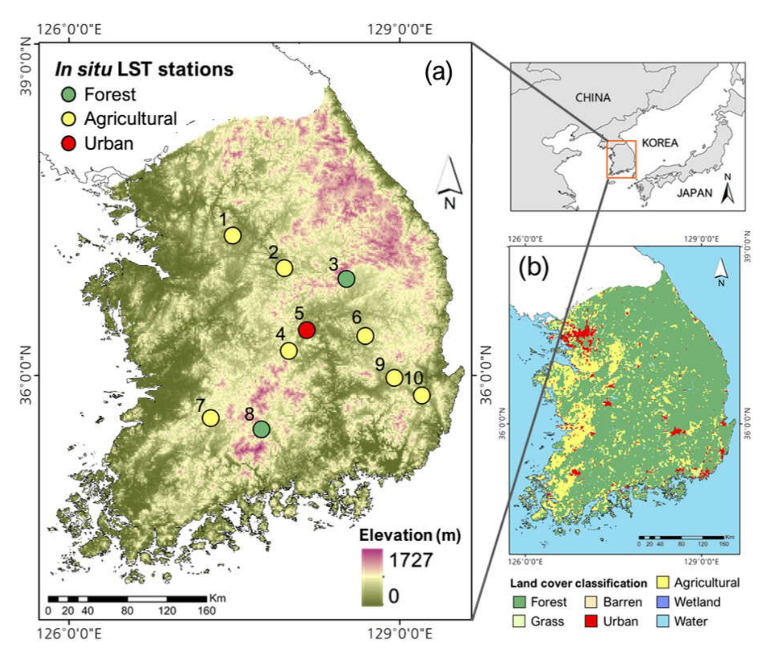
The study area is the mainland of South Korea with an area of approximately 99,728 km² (latitude 34° N–38.5° N and longitude 126° E–129.5° E) (Figure 1). South Korea generally has a humid, continental climate affected by the Asian monsoons, with a large amount of precipitation in summer during the rainy season (usually from the end of June to the end of July). The annual mean temperature is about 10–15 °C; August, the hottest month, has a mean temperature of 23–26 °C. Humidity ranges from 60%–75% on a national scale, with summers (July and August) rising to 70%–85%. The southern coast is subject to late-summer typhoons. As seen in Figure 1, the dominant land-cover categories of the study area are forest (67.7%), agricultural land (22.2%), urban areas (4.6%), and others, including grass, water, barren, and wetlands (5.5%).

2.2. Saetellite Data

The AMSR2 onboard the global change observation mission 1st-water (GCOM-W1) satellite, launched in May 2012, provides global PMW-based BT data. It acquires a set of daytime and nighttime microwave data twice a day: The equator crossing time is 1:30 p.m. for the ascending pass, and 1:30 a.m. for the descending pass. The AMSR-2 has seven frequencies, with both vertical and horizontal polarizations, and approximately 62 × 35, 62 × 35, 42 × 24, 22 × 14, 19 × 11, 12 × 7, and 5 × 3 km spatial resolution at 6.9, 7.3, 10.7, 18.7, 23.8, 36.5, and 89.0 GHz, respectively. Among these, we used the four frequencies (36.5, 23.8, 18.7, and 10.7 GHz) mostly used for the estimation of LST in the previous studies [30]. Low frequency data resampled into a 10 km resolution were downloaded from the Japan Aerospace Exploration Agency (https://gcom-w1.jaxa.jp) for 2013–2018. We used daily MODIS daytime and nighttime Aqua LST data (MYD11A1) because the equatorial-crossing times of Aqua MODIS are nearly the same as those of AMSR2 (1:30 p.m.–daytime and 1:30 a.m.–nighttime). The MYD11A1 LST data, which have 1 km spatial resolution, were retrieved using a generalized split-window algorithm [33]. The MYD11A1 products from 2013–2018 were downloaded from Earthdata Search (https://search.earthdata.nasa.gov/search). South Korea’s elevation was retrieved from the shuttle radar topography mission (SRTM) digital elevation model (DEM), with 30 m spatial resolution (https://earthexplorer.usgs.gov). Global man-made impervious surface (GMIS) data with 30 m spatial resolution derived from Landsat images for the year of 2010 [34] were obtained to get the fractional impervious surface in this study.

2.3. In Situ LST Data

In situ LSTs (1 a.m./p.m. and 2 a.m./p.m.) from 2013 to 2018, obtained from the automated surface observing systems (ASOSs) operated by the Korea Meteorological Administration, were used as reference data. As shown in Figure 1a, a total of 10 ASOSs were selected based on the following conditions: First, the stations close to the coastline were excluded, because satellite-based LST data could be contaminated from the influence of ocean water included in the grid; and second, the stations that have high bias were also excluded from the reference data, after applying the bias-correction method described in Section 3.1.

3. Methods

3.1. LST Pre-Processing

The 1 km MODIS LSTs with quality control (QC) flags of ‘cloud’ were considered to be pixels under cloudy sky conditions, and all others were clear sky LSTs. To train the model and validate the estimated LST under cloudy areas, we used in situ LSTs measured at ASOSs. However, there are spatial scale differences between the MODIS LST (1 km) and the point-based ASOS LST; thus, a systematic bias could occur. To solve this problem, we fitted in situ LST and MODIS LST under clear sky conditions using polynomial regression by station [35], to bias-correct in situ LSTs for both daytime and nighttime (Equation (1)).

$$\mathrm{Y}={\mathrm{aX}}^2+\mathrm{bX}+\mathrm{C}$$

(1)

where X is the in situ LST and Y is the MODIS LST under clear sky conditions. a, b, and c represent the coefficients. We used the quadratic function because many ASOSs have observed that in situ LSTs rise more rapidly than MODIS LSTs at high temperatures in the summertime.

The MODIS and in situ LSTs from March to October, starting from 2013 through to 2018 at each station were used for the bias-correction. Only MODIS LSTs with good quality were used based on the QC flags, and the hourly in situ LSTs were linearly interpolated to the MODIS view time. We excluded the winter season (December through February) because the range of winter LSTs is not compatible with that of summer LSTs, which are the target variable of this study. Finally, we selected a total of 10 ASOSs for validation, with a calibration error (RMSE) < 2.5 °C for both daytime and nighttime in July–August (summer season) from the bias-correction analysis. Figure 1 shows the geographic distribution of the ten ASOSs used in this study. Appendix A1 describes the statistical results of before and after bias correction of the 1 km in situ LSTs at the 10 stations.

In addition, clear sky 1 km MODIS LSTs were aggregated to 10 km based on the 10 km AMSR2 grid area. At this stage, only 1 km MODIS LSTs where 95% or more clear sky LSTs exist in a 10 × 10 km² area were used for aggregation. We also fitted the in situ LSTs and the 10 km MODIS LSTs under clear sky conditions using polynomial regression in the same way as the bias correction of the 1 km LSTs at the selected 10 ASOS stations to produce the bias-corrected in situ LSTs at 10 km scale.

3.2. Pre-Processing of Input Variables

Table 1. Description of input variables used in this study.

Type	Variables	Acronym
AMSR2 BT	36.5 GHz horizontal polarization	36H
	36.5 GHz vertical polarization	36V
	23.8 GHz horizontal polarization	23H
	23.8 GHz vertical polarization	23V
	18.7 GHz horizontal polarization	18H
	18.7 GHz vertical polarization	18V
	10.7 GHz horizontal polarization	10H
	10.7 GHz vertical polarization	10V
Annual cycle parameters	Mean annual LST (K)	MAST
	Mean annual amplitude of LST (K)	YAST
	Phase shift relative to spring equinox on the Northern hemisphere	theta
Auxiliary variables	Elevation (m)	Elev
	Impervious surface fraction (%)	Imp
	Latitude (°)	Lat
	Longitude (°)	Lon
	Converted day of year	DOY
	Year as a discrete value	Year

describes the input variables used for the estimation of LST under cloudy conditions. A total of 10 AMSR2 BTs were projected onto MODIS LSTs, whilst AMSR2 pixels from near the coastline were masked to eliminate the effects of ocean water. Due to the shift of the flight overpass path, the areas of missing AMSR2 BT values were also excluded.

The 1 km MODIS annual cycle parameters (ACPs), including mean annual surface temperature (MAST), yearly amplitude surface temperature (YAST), and LST phase shift relative to the spring equinox (theta) were calculated for each of daytime and nighttime based on the following equation [36].

$$\mathrm{f}\left(\mathrm{d}\right)=MAST+YAST *\sin \left(\frac{d2\pi }{365}+theta\right)$$

(2)

where d represents the day of the cycle relative to the spring equinox. The ACPs were created for each year of the study period and averaged to construct one MAST, YAST, and theta each for daytime and nighttime.

We aggregated the 30 m SRTM elevation and 30 m GMIS impervious surface fraction to the 1 km resolution of MODIS. Latitude and longitude values were extracted from the information contained in the MODIS tiles. This study converted DOY to values ranging from −1 to 1 within a one-year period, using a sine function that considers seasonality (i.e., setting the middle of summer as 1 and the middle of winter as −1) [37].

3.3. Random Forest (RF)

In this study, we applied machine-learning random forest (RF) to estimate the LST for all-weather conditions. RF has been widely used to conduct a variety of classification and regression tasks [38,39,40,41,42,43]. RF comprises classification and regression trees, producing a variety of independent trees to make a final decision through two randomizations: (1) Random selection of training samples and (2) random selection of predictor variables at each node of a tree [44]. This randomization is aimed at solving the overfitting problem and reducing the sensitivity of a model that comes from training sample configurations [45]. When a variable is randomly permuted, RF calculates the relative variable importance from out-of-bag (OOB) samples, measuring the mean squared error (MSE) of the OOB portion of samples in each tree. The same process is implemented whenever each input variable is perturbed, and the difference between the two MSEs of all trees is averaged. The larger the increase in the percentage of MSE (%incMSE) of a variable, the greater the contribution of the variable. It should be noted that the relative variable importance is considered as the sum of local contributions, not global importance [46,47,48]. The RF was implemented using the R statistical software through the “ranger” add-on package, with default model parameter settings (e.g., the number of trees set as 500). The “ranger” is a fast implementation of RF, or recursive partitioning, and is known to be suited to high-dimensional data with large datasets [49].

3.4. Schemes for Estimating All-Weather LSTs

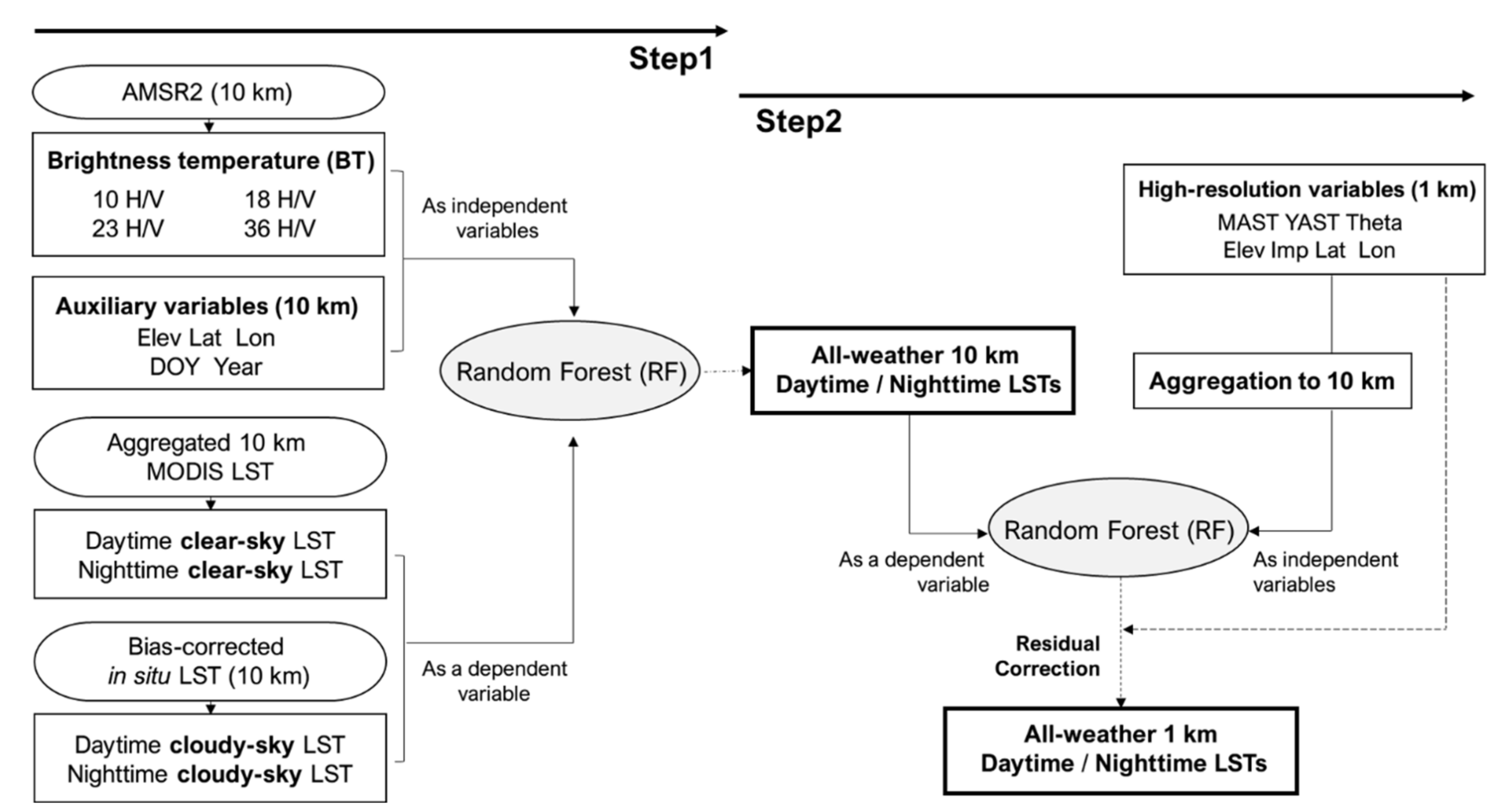
In this study, we proposed two schemes (S1 and S2) to estimate all-weather MODIS LSTs. The S1 is based on a two-step approach (see Figure 2). The first step is estimating 10 km LSTs for daytime and nighttime. We used the following independent variables: Four different frequencies of the AMSR2 of two polarization BTs (10H/V, 18H/V, 23H/V, and 36H/V), along with five 10 km resampled auxiliary variables (Elev, Lat, Lon, DOY, and year). The aggregated 10 km MODIS LSTs under the clear sky condition were used as a target variable. Moreover, we used the 10 km bias-corrected in situ LSTs under the cloudy sky condition from 10 stations as a dependent variable together to train the model with the real LST characteristics under the cloudy skies. RF was applied to predict LSTs by training the samples from March to October between 2013 and 2018. Finally, the 10 km LSTs were produced based on the developed model using the input variables under all-weather conditions.

The second step involved the spatial downscaling of LSTs from 10 km to 1 km. We used RF to develop the downscaling model for each date. The Elev, Imp, Lat, Lon, and ACPs (i.e., MAST, YAST, and theta) were used as input variables, considering the surface properties and spatial distribution characteristics of 1 km LSTs. At first, the 1 km MAST, YAST, and theta with 1 km auxiliary factors—Elev, Imp, Lat, and Lon—were aggregated to 10 km for independent variables for the RF model, and the 10 km LSTs, constructed in the first step, were used as the dependent variable. After the model was trained for each date, the original high-resolution 1 km input variables were put into the RF model to finally produce the 1 km all-weather LSTs, after the residual correction proposed by Hutengs and Vohland [50].

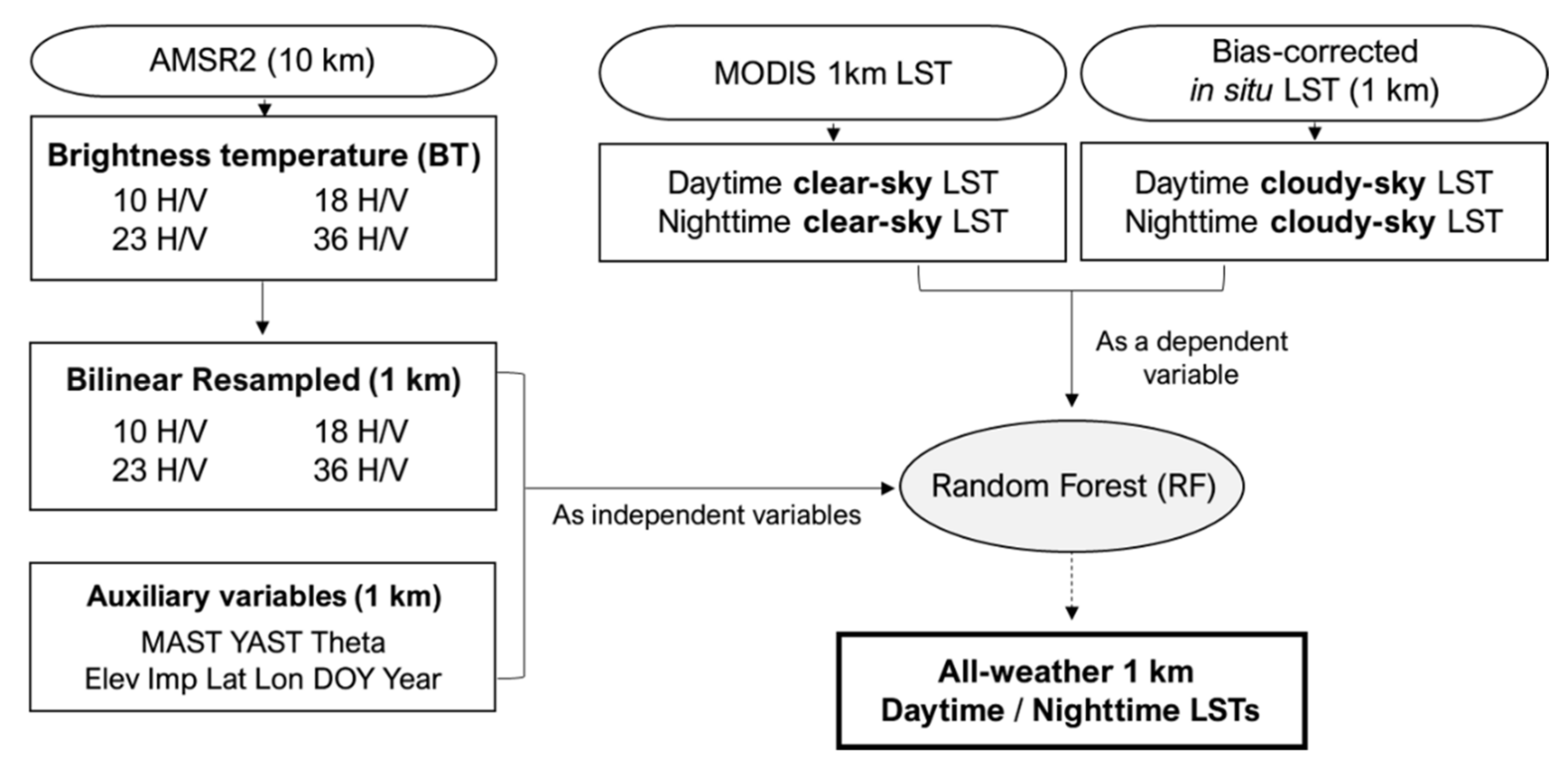
The second scheme S2 is a one-step algorithm that directly estimates 1 km all-weather LSTs (Figure 3). To create this scheme, first we downscaled all 10 km AMSR2 BTs to 1 km using bilinear resampling. The resampled BTs together with 1 km auxiliary variables (i.e., MAST, YAST, theta, Elev, Imp, Lat, Lon, DOY, and Year) were used as input variables in RF. We used the 1 km clear sky MODIS LSTs and the 1 km bias-corrected in situ LSTs under cloudy skies from ten stations as target variables for daytime and nighttime separately. RF models were built for each year with the samples of the entire study area from March through October being used for training. We put the input variables of all-weather conditions into the developed RF model to produce 1 km LSTs for both clear and cloudy sky conditions.

3.5. A Series of Validations

For the first step of the first scheme, S1, two types of validations were implemented using the clear sky 10 km aggregated MODIS LSTs focusing on the summertime (i.e., July and August). In the first validation, we randomly divided July and August samples into training and validations sets (80%/20% split). In the humid summer, however, most of the area in South Korea is often covered by clouds for the whole day. So, for the second validation, we randomly divided the samples of July and August by date: 80% for training and the remaining 20% for validation. In the second step of S1, LSTs downscaled into 1 km by RF were validated using all clear sky MODIS LSTs in the summer. At this stage, we compared the performance of RF with other downscaling techniques in two ways: (1) A bilinear resampling of 10 km LSTs to 1 km; (2) a lapse-rate technique using Equation (3), which assumes that the temperature difference comes from elevation, suggested by Dual et al. [12]:

$$LS{T}_{1 km}=TLR\times \left(El{v}_{1 km}-El{v}_{10 km}\right)+LS{T}_{10 km}$$

(3)

where LST_1km is the downscaled LST at 1 km scale; LST_10km represents the predicted 10 km LSTs in step 1; Elv_1km is the surface elevation at 1 km scale; Elv_10km is the surface elevation at 10 km scale; and the TLR is the temperature lapse rate, which is defined as the rate of temperature decrease with elevation in the troposphere (average TLR value is 6.5 K/km; [51]). For the second scheme, S2, first and second validations similar as in S1 were performed.

Moreover, the estimated all-weather 1 km LSTs, including those under cloudy skies, were validated using bias-corrected in situ LSTs of 10 ASOSs in summer. Among the 10 ASOS stations, data at one station were used as validation and the others were used to train the model with in situ cloudy LSTs as targets. This leave one-station out cross-validation (LOOCV) was repeated for all 10 stations. The coefficient of determination (R²; Equation (4)), RMSE (Equation (5)), normalized RMSE (nRMSE; Equation (6)), and bias (Equation (7)) were used to evaluate the performance of the models for each validation step.

$${\mathrm{R}}^2=1-\frac{{{\displaystyle \sum }}_{i=1}^n{\left(y_i-{\widehat{y}}_i\right)}^2}{{{\displaystyle \sum }}_{i=1}^n{\left(y_i-\overline{y}\right)}^2} , \overline{y}=\frac{1}{n}{{\displaystyle \sum }}_{i=1}^n{y}_i ,$$

(4)

$$\mathrm{RMSE} (°\mathrm{C})=\sqrt{{\displaystyle \sum }_{i=1}^n\frac{{\left({\widehat{y}}_i-y_i\right)}^2}{n}} ,$$

(5)

$$\mathrm{nRMSE} (\%)=\frac{\mathrm{RMSE}}{\left(y_{max}-y_{min}\right)}\times 100 ,$$

(6)

$$\mathrm{Bias} (°\mathrm{C}) ={{\displaystyle \sum }}_{i=1}^n\frac{\left({\widehat{y}}_i-y_i\right)}{n} ,$$

(7)

where $y_i$ is the measured value, ${\widehat{y}}_i$ is the predicted value, $y_{max}$and $y_{min}$ represent the maximum and minimum values of observations, and n is the number of samples.

4. Results and Discussion

4.1. Analysis of Clear and Cloudy Sky in Situ LSTs in Summer

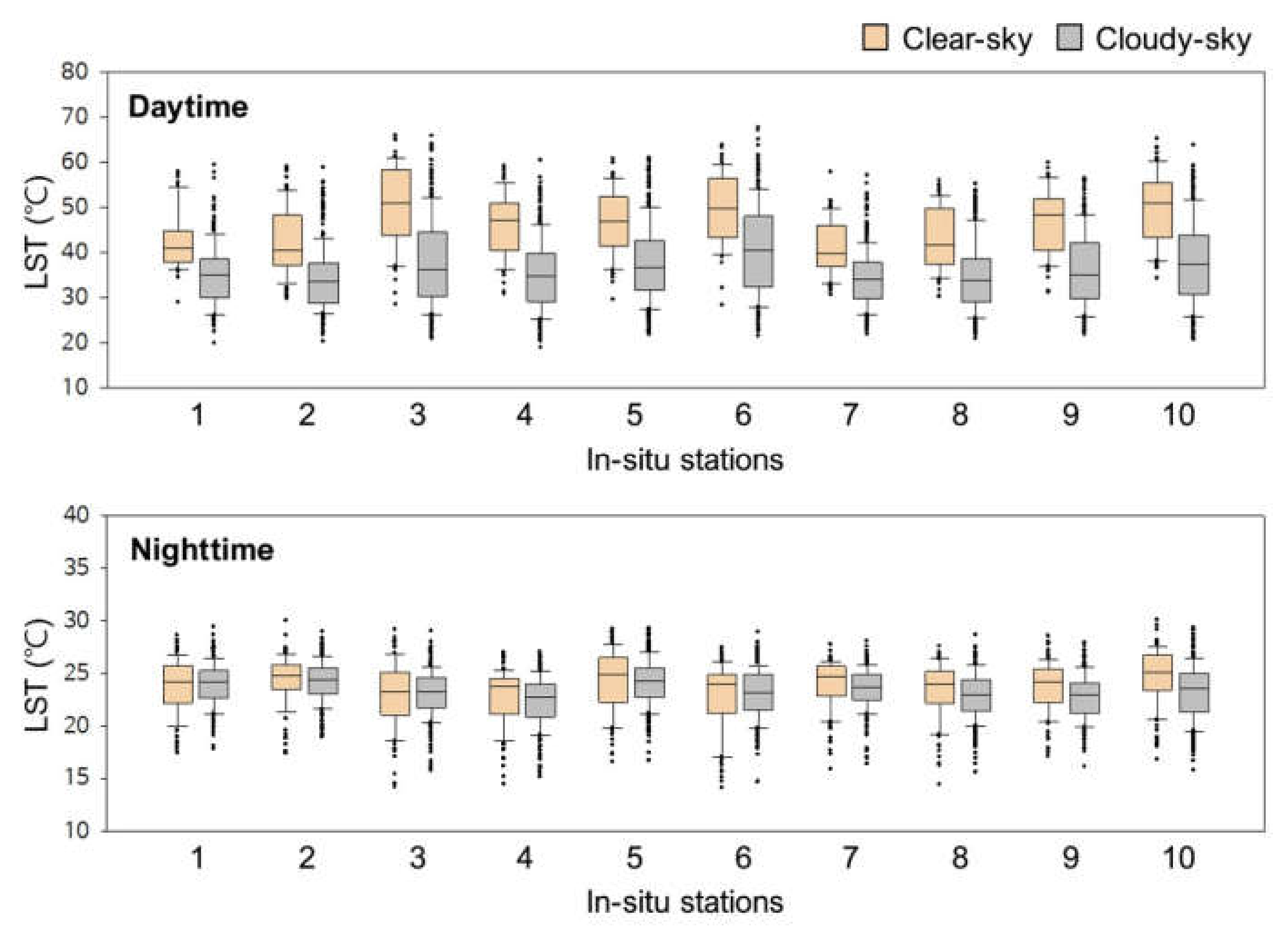
Figure 4 depicts the boxplots of bias-corrected LSTs for the 10 in situ stations under clear sky and cloudy sky conditions. It should be noted that the average LSTs in clear skies were higher than those of cloudy skies for all stations in the daytime. Although high LSTs also appear under cloudy sky conditions, LSTs are considerably lower when compared to clear sky LSTs. The boxplot (Figure 4) shows that the upper quartile of cloudy sky LSTs is close to the lower-quartile of clear sky LSTs for most in situ stations. One possible reason for this is an increasing cloud-cover on rainy days in humid areas in the summer, where precipitation reduces the surface sensible heat [12,52]. When the sky is heavily cloudy in the daytime, most of the Sun’s energy does not reach the surface, preventing the heating up of the Earth. Otherwise, at nighttime, clear sky and cloudy sky LST distributions do not differ significantly for all the stations. There is no incoming radiation from the Sun at night, therefore LSTs do not rise significantly. The average nighttime LSTs—early overnight—under cloudy skies have a nearly identical range as, or only slightly lower than, the clear sky LSTs.

Among the 372 days, the total number of summer days (July–August) for the six years (2013–2018), the size of good-quality clear sky samples was very small, especially for the daytime (see the sample size in

Table A1. The relationship between clear sky MODIS LSTs and the before-and-after 1 km bias-corrected in situ LSTs during July and August from 2013 to 2018 for the 10 stations in daytime. Refer to Figure 1 for station numbers.

Station Number	Before Bias-correction			After Bias-correction			Sample Size
	R2	RMSE (°C)	Bias (°C)	R2	RMSE (°C)	Bias (°C)
1	0.62	10.50	8.89	0.64	1.88	−0.06	15
2	0.75	9.01	7.29	0.74	2.00	−1.05	16
3	0.64	18.49	17.71	0.64	2.20	−0.12	26
4	0.65	14.23	13.43	0.66	1.97	−0.20	30
5	0.56	11.41	10.31	0.67	2.38	−0.09	15
6	0.61	17.45	16.92	0.60	2.12	−0.51	16
7	0.57	9.55	8.15	0.59	2.06	0.15	21
8	0.46	11.37	10.30	0.46	2.39	−1.19	27
9	0.76	11.22	10.38	0.77	1.99	−0.74	15
10	0.54	16.43	15.20	0.53	2.15	−0.43	23

and

Table A2. The relationship between clear sky MODIS LSTs and the before-and-after 1 km bias-corrected in situ LSTs during July and August from 2013 to 2018 for the 10 stations at nighttime. Refer to Figure 1 for station numbers.

Station Number	Before Bias-correction			After Bias-correction			Sample Size
	R2	RMSE (°C)	Bias (°C)	R2	RMSE (°C)	Bias (°C)
1	0.77	3.34	3.02	0.78	1.38	0.01	58
2	0.72	2.60	2.27	0.72	1.28	0.02	34
3	0.78	2.99	2.64	0.79	1.14	−0.05	55
4	0.85	2.37	2.10	0.86	1.01	0.01	48
5	0.84	2.54	2.24	0.84	1.11	0.02	46
6	0.83	2.30	1.88	0.83	1.21	0.03	67
7	0.66	3.96	3.74	0.66	1.30	0.06	59
8	0.52	3.37	3.00	0.52	1.46	0.10	62
9	0.69	2.42	1.91	0.70	1.47	0.10	49
10	0.70	2.96	2.55	0.70	1.29	0.00	71

). This implies that the temporal or spatial interpolation approach to reconstructing LSTs in cloudy conditions could not be effectively applied to the summer season because of a large amount of cloud contamination.

4.2. Evaluation of Two Schemes Using Clear Sky LSTs

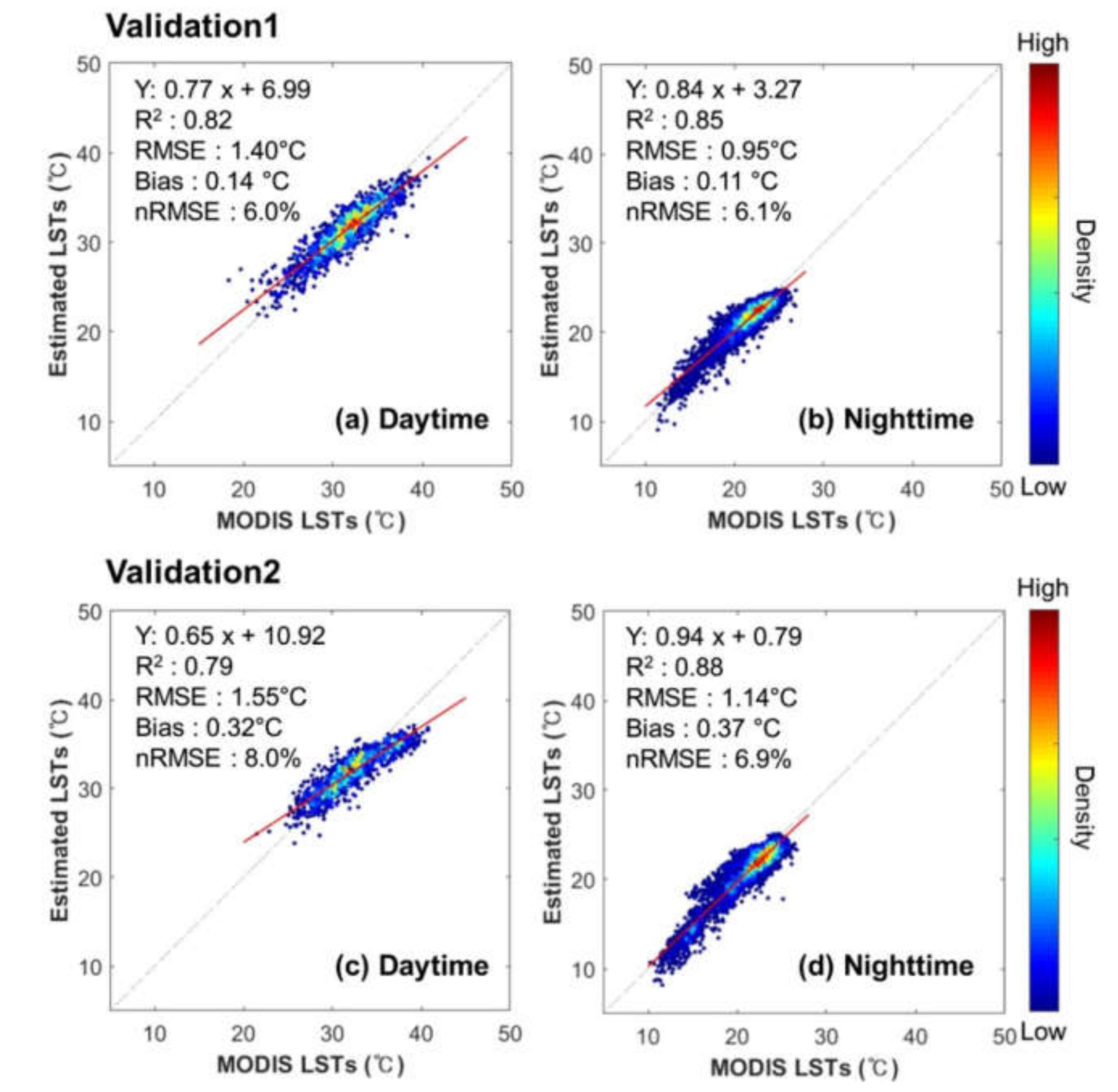
Figure 5 shows the results of the first (upper) and second (lower) validations for summer daytime and nighttime for Scheme 1(S1). The R² values for estimating 10 km daytime and nighttime LSTs were 0.82 and 0.85, respectively, in the first validation. The RMSE values have a daytime LST of 1.40 °C and a nighttime LST of 0.95 °C. Considering their similar nRMSE, the main reason for the RMSE difference between daytime and nighttime is likely the range difference in the temperature distribution. In the second validation, the R² (RMSE) values for estimating 10 km daytime and nighttime LSTs were 0.79 (1.55 °C) and 0.88 (1.14 °C), respectively. The accuracy of the two RF-based validations corresponds to the MODIS LST validation error of 1–2 K [53,54,55]. In particular, the second validation results were similar to the first validation in terms of accuracy (i.e., R² and nRMSE), even with a separate validation dataset by date. These results imply that the constructed 2-step RF-based model is robust for humid areas where clouds often cover most regions in summer. However, since we performed both validations using the MODIS clear sky LSTs, the effect of clouds was not considered. Thus, accuracy assessment using in situ LST data under cloudy conditions was needed.

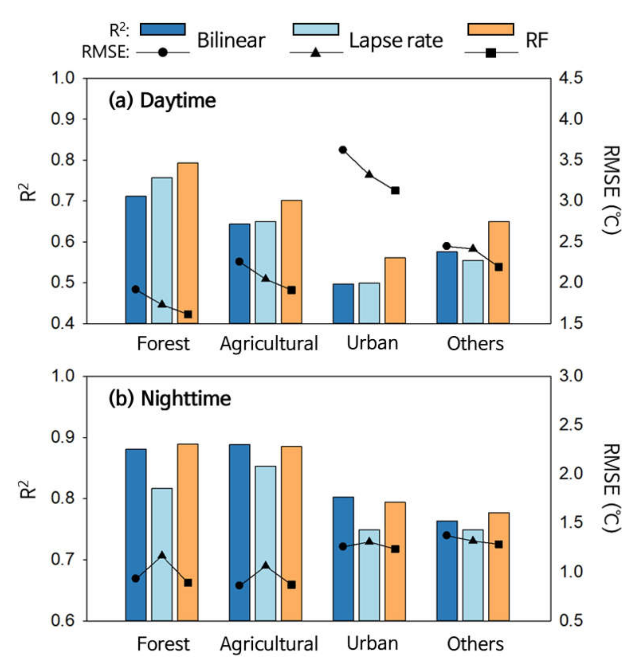
Figure 6 shows the validation results of the second step for Scheme 1, using clear sky MODIS LSTs estimated with the bilinear resampling (Bilinear), the lapse rate approach (Lapse rate), and the proposed RF-based algorithm (RF) among the different land covers. RF outperformed the other two techniques with higher correlation and lower RMSE in most land covers for both daytime and nighttime. For daytime, RF showed R² of 0.6–0.8 and RMSE of 1.6–3.0 °C with some variation according to land cover. This accuracy is considered significant with an average range value of RMSE similar to approximately 2.0 K, which is the target accuracy in several daytime LST retrieval studies [56,57,58]. The reason why urban areas showed lower performance than other land covers might be that the relatively high LSTs in urban areas were not accurately simulated when downscaling 10 km LST to 1 km, considering the fact that RF underestimated the downscaled LSTs (mean bias: −1.5 °C, not shown). Moreover, it has been reported that MODIS daytime LSTs in urban areas have relatively high uncertainty [16,59]. Note that the RF outperformed the lapse rate approach, which assumes the dependency of cloudy LSTs only on the altitude for all land covers in the daytime [12]. The RF appears to simulate the surface thermal heterogeneity well in daytime, using not only Elev, but also the Imp and ACPs—MAST, YAST, and theta—as input variables.

For nighttime, the RF model returned highly accurate results, with R²~0.8 to 0.9 and RMSE < 1.5 °C with some variations by land cover. The lapse rate approach showed worse performance than the other two methods for most land cover types. Duan et al. used an average lapse rate of 6.5 K/km for both day and night [12]. However, the lapse rate could be applied to the air temperature of the troposphere, not the LSTs, which implies that the LST difference by altitude does not seem to be significant on the local scale. Interestingly, the bilinear and RF models did not show much difference for nighttime, where RF showed slightly better performance than the bilinear interpolation in terms of R² and RMSE for most land covers. This suggests that the nighttime LST is thermal-homogenous enough for bilinear interpolation to achieve good results.

Table 2. The two validation results of the 1 km LST estimation from scheme 2(S2) for daytime and nighttime.

Daytime	R2	RMSE (°C)	nRMSE (%)	Bias (°C)	Sample Size
Validation1	0.93	0.97	3.2	0.00	139,876
Validation2	0.79	1.62	5.9	0.16	138,307
Nighttime	R2	RMSE (°C)	nRMSE (%)	Bias (°C)	Sample Size
Validation1	0.96	0.53	2.7	0.02	353,114
Validation2	0.79	1.07	6.5	0.03	298,575

summarizes the results of the first and second validations for a 1 km clear sky LST estimation in S2. The first validation showed excellent performance resulting in R² > 0.9 and RMSE < 1 °C for both daytime and nighttime. The second validation, however, dividing samples by date, yielded relatively low accuracy, which is possibly due to the daily LST variations. It is not surprising that the prediction performance of S2 by time over humid areas in the summer would be less accurate than the first validation, because clouds covered most areas for specific days, which might not have been trained well. In particular, cloudy areas in the summer daytime have an LST range different from clear sky areas (Figure 4); therefore, S2-based 1 km LSTs need further investigation using in situ data under cloudy conditions.

4.3. Spatial Distribution Analysis of All-weather LSTs from Two Schemes

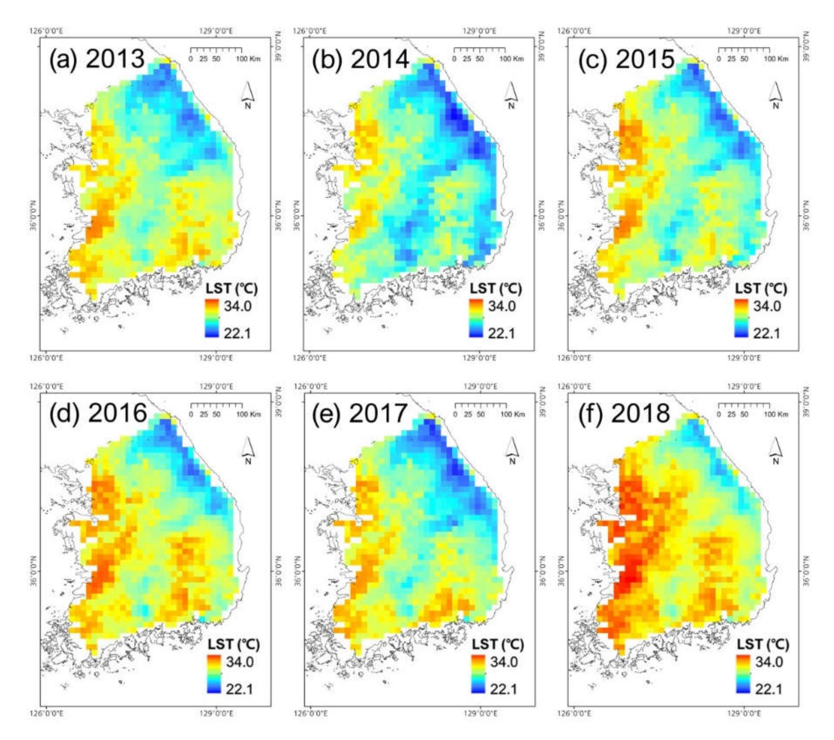
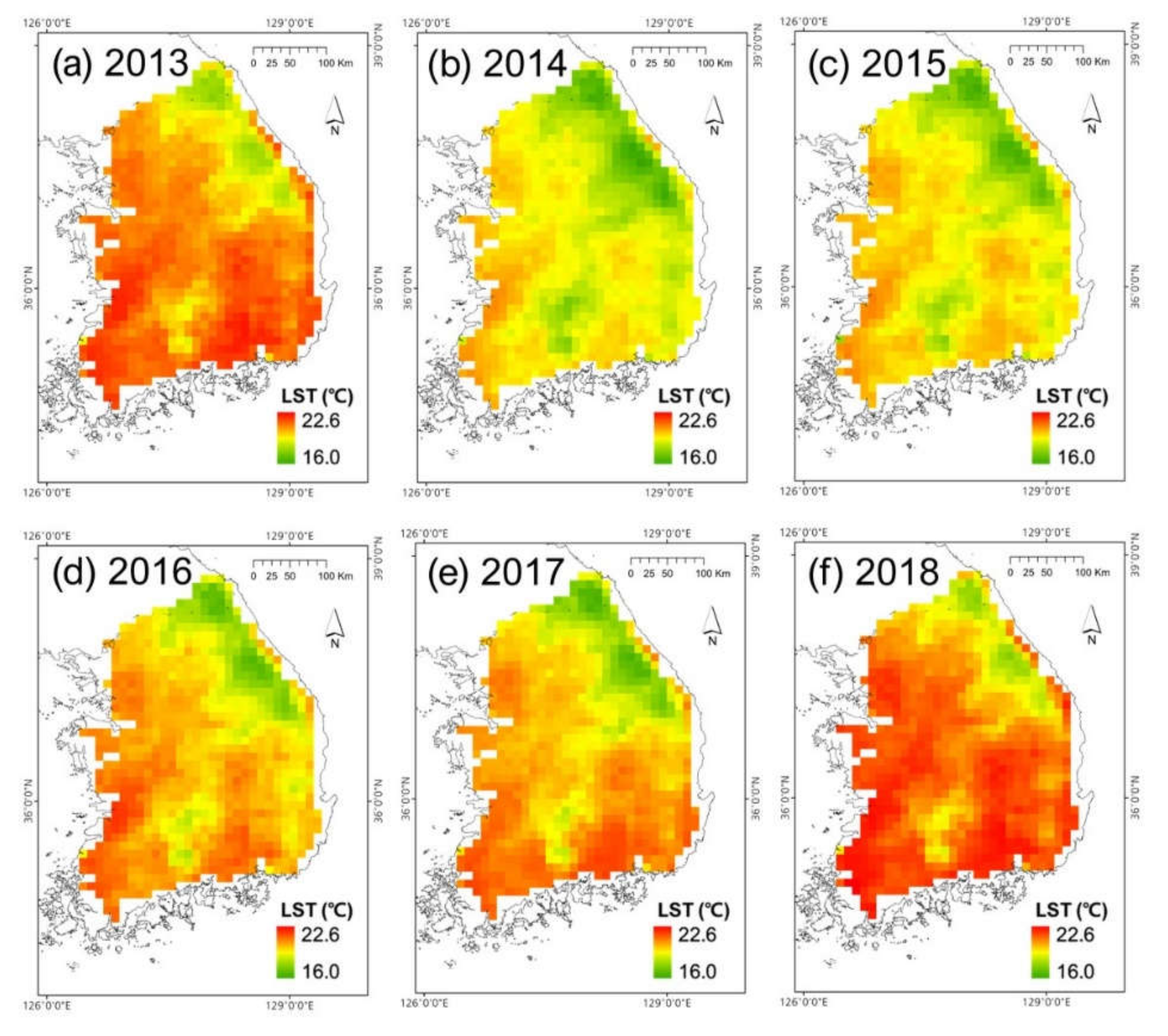
Figure 7 and Figure 8 show the all-weather average daytime and nighttime 10 km LSTs of S1 from July through August for each year. The overall spatial distribution of the daytime and nighttime LSTs appeared similar, but the range of the daytime LSTs (22.1–34.0 °C) was considerably higher than that of the nighttime LSTs (16.0–22.6 °C). This is because the differences in heat capacity and evapotranspiration by land type result in a wide range of LSTs in the daytime, affected by incoming solar radiation [22]. Elevation (see Figure 1) yielded a negative spatial relationship with LSTs for both daytime and nighttime, which is consistent with the results of Bertoldi that showed that LST decreases with increasing elevation because of complex factors such as air temperature and vegetation amount [60]. In this study, therefore, the elevation input variable contributes significantly to the LST estimation model. In terms of land cover (see Figure 1), LSTs were relatively low in both the daytime and nighttime in the forested areas, widely distributed in the study area. Meanwhile, the cropland areas showed higher temperature values than in forests, especially for the western part of the study region, which is consistent with the results of Lee et al. [61]. The urban areas also showed relatively high LSTs compared to other landcovers, because of the highly impervious surfaces in both daytime and nighttime [32,62].

The developed 10 km LSTs of S1 also showed a temporal variation over six years (2013–2018). For example, South Korea experienced unprecedented extreme temperatures (i.e., a heatwave) in the summer of 2018 [63], where the developed LSTs show distinctly high-temperature distribution for both daytime and nighttime (Figure 7f and Figure 8f). Furthermore, 10 km LSTs were relatively high at nighttime of summer 2013 (Figure 8a), which is consistent with the analysis of Choi and Lee that showed frequent tropical night events in South Korea in summer 2013 [64]. Overall, the LSTs estimated using S1 on the 10 km scale seem to accurately describe both spatial and temporal patterns of LSTs in summer daytime and nighttime.

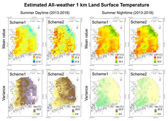
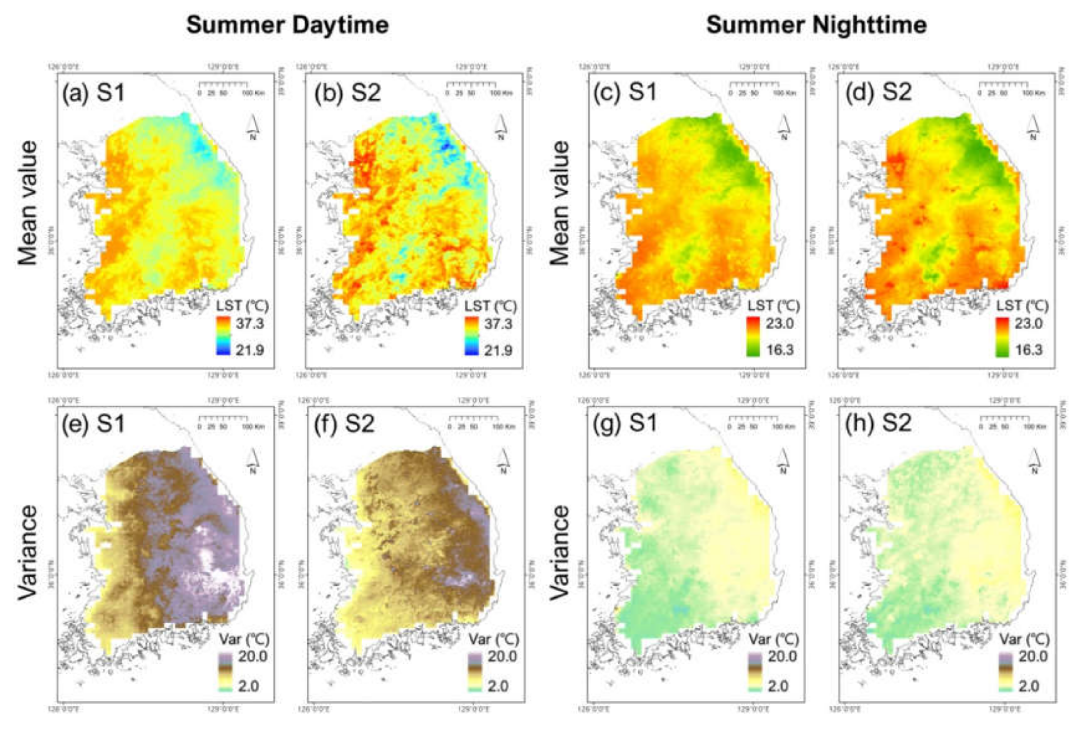
Figure 9 shows the mean and variance of the 2013–2018 1 km all-weather LSTs produced by S1 and S2 for summer in both the daytime and nighttime. In the daytime, it should be noted that S2 generally simulated LSTs higher in urban and agricultural areas than S1 (Figure 9a,b). The difference in the estimated LSTs between S1 and S2 might also be due to S2 overestimating the low LSTs under cloudy conditions. The bias of the second validation of daytime was relatively high (~0.16), as shown in Table 2. At nighttime, the S1 and S2 showed similar LST distributions, except urban areas where the S1 LSTs were slightly higher than the S2 ones.

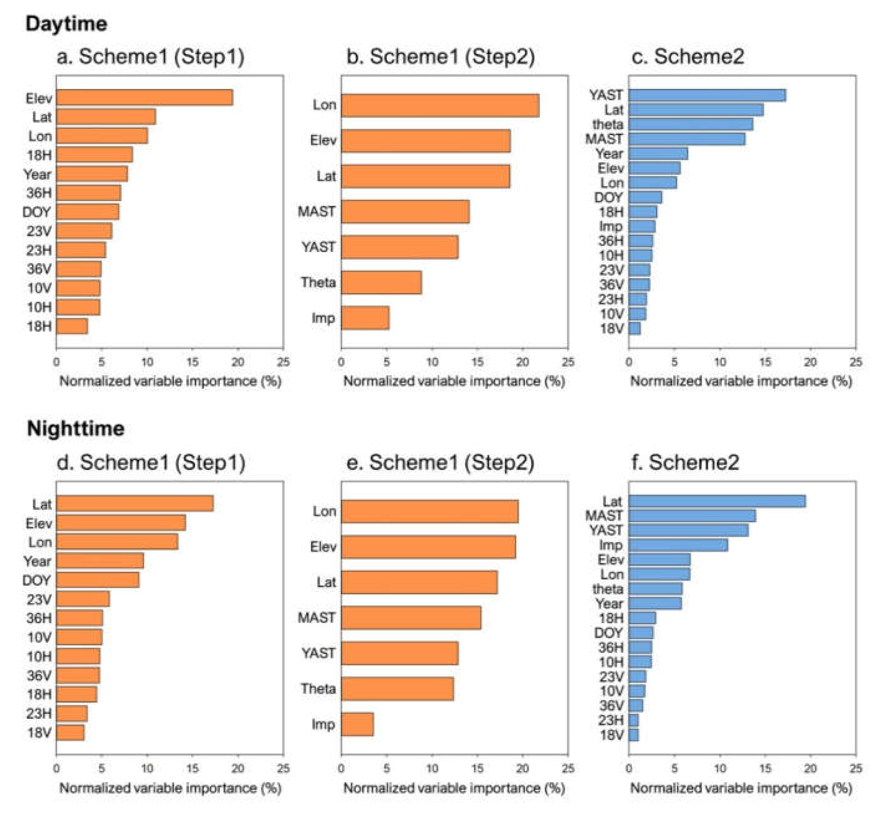
Note that the variance of S1 LSTs is quite a lot higher than S2 in most areas in the daytime (Figure 9e–f). The relative variable importance (%) explains this fact as provided by RF (Figure A1). Among the several input variables, only AMSR2 BTs showed temporal changes. In S2, temporally constant variables, such as Lat, YAST, theta, and MAST, played significant roles in the RF model (Figure A1c); therefore, S2 could be relatively limited in simulating the temporal variations of LSTs. In the case of S1, AMSR2 BTs were used only to construct the 10 km LSTs first (step 1), whereas ACPs were used only for step 2. Therefore, S1 could simulate the temporal pattern of daily LSTs accurately by downscaling the proposed 10 km LSTs to 1 km for each day in step 2. At nighttime, S1 and S2 had similar LST variance for most areas (Figure 9g–h). In particular, LSTs in summer nighttime have a distinctly lower variance than those in the daytime (Figure 9e–f), which implies that the nighttime does not show significant temperature changes in summer regardless of weather conditions.

Many previous studies that predicted 1 km cloudy sky LSTs have used auxiliary variables that are indirectly related to LST, such as elevation, latitude, and longitude [12,19]. It should be noted that ACPs (i.e., MAST, YAST, and theta) have been identified as crucial variables by RF for both S1 and S2 (Figure A1). This suggests that ACPs are useful in estimating LSTs for all-weather conditions, due to their characteristics representing the spatial distribution of LSTs, without being affected by clouds.

4.4. Comparison of Two Schemes Using in Situ LSTs

The clear and cloudy sky 1 km LSTs produced from the two schemes were validated (i.e., LOOCV) using the 1 km bias-corrected in situ LSTs measured at the 10 stations (

Table 3. The leave one-station out cross-validation (LOOCV) results of the estimated 1 km clear and cloudy sky LSTs from scheme 1 (S1) and scheme 2 (S2) using bias-corrected in situ LSTs at 10 stations during July and August from 2013 to 2018 for daytime. Refer to Figure 1 for station numbers.

Station	Clear Skies						Cloudy Skies
	R2		RMSE (°C)		Bias (°C)		R2		RMSE (°C)		Bias (°C)
	S1	S2	S1	S2	S1	S2	S1	S2	S1	S2	S1	S2
1	0.54	0.58	2.6	1.9	−1.7	0.3	0.77	0.76	2.2	2.7	−1.2	1.9
2	0.63	0.72	2.5	1.7	−1.6	0.4	0.73	0.67	2.6	2.4	−1.5	1.1
3	0.71	0.73	3.9	2.8	−3.0	1.1	0.74	0.65	2.9	5.6	−0.1	4.6
4	0.73	0.76	1.7	1.7	−0.6	0.9	0.73	0.67	2.1	3.3	0.0	2.4
5	0.65	0.64	4.9	1.8	−4.5	0.1	0.81	0.77	3.9	3.2	−3.2	2.1
6	0.76	0.64	2.8	4.0	−0.1	2.5	0.81	0.80	2.9	5.8	1.6	5.2
7	0.63	0.65	2.2	1.5	−1.8	0.7	0.82	0.79	2.2	1.7	−1.8	0.9
8	0.56	0.64	2.2	2.3	0.1	1.2	0.81	0.77	2.1	3.5	1.2	2.9
9	0.74	0.71	3.8	2.3	−3.3	1.1	0.81	0.80	2.4	5.1	−0.2	4.4
10	0.44	0.48	1.9	2.1	−0.4	1.1	0.80	0.75	2.5	4.7	1.0	4.0

for daytime and

Table 4. The leave one-station out cross-validation (LOOCV) results of the estimated 1 km clear and cloudy sky LSTs from scheme 1(S1) and scheme 2(S2) using 1 km bias-corrected in situ LSTs for 10 stations during July and August from 2013 to 2018 for nighttime. Refer to Figure 1 for station numbers.

Station	Clear Skies						Cloudy Skies
	R2		RMSE (°C)		Bias (°C)		R2		RMSE (°C)		Bias (°C)
	S1	S2	S1	S2	S1	S2	S1	S2	S1	S2	S1	S2
1	0.92	0.89	0.7	0.9	0.1	0.2	0.70	0.68	1.3	1.3	−0.7	−0.8
2	0.89	0.87	1.3	1.0	−1.0	−0.5	0.68	0.64	2.2	2.0	−1.9	−1.7
3	0.87	0.82	1.0	1.2	−0.4	−0.2	0.71	0.70	1.9	1.9	−1.5	−1.5
4	0.87	0.87	0.9	0.8	0.1	0.0	0.74	0.73	1.3	1.4	−0.8	−0.9
5	0.90	0.88	1.2	1.0	−0.7	−0.3	0.63	0.69	2.1	1.8	−1.6	−1.4
6	0.87	0.85	1.0	1.0	0.3	0.1	0.60	0.60	1.5	1.6	−0.8	−0.9
7	0.83	0.81	0.9	0.9	0.5	0.2	0.69	0.69	1.0	1.1	−0.1	−0.3
8	0.76	0.71	1.0	1.1	0.2	0.1	0.70	0.71	1.1	1.2	−0.4	−0.5
9	0.84	0.84	1.0	1.0	−0.3	0.0	0.68	0.68	1.7	1.7	−1.2	−1.1
10	0.87	0.82	0.7	1.0	0.1	0.1	0.70	0.72	1.4	1.4	−0.7	−0.7

for nighttime). It should be noted that S1 showed negative biases for most stations, which implies that S1 tended to underestimate 1 km LSTs under clear sky conditions. In particular, the RMSE of S1 was relatively high with a large negative bias, especially for stations 5. This might be because the station was located in built-up urban areas, where S1 LSTs were possibly underestimated, as presented in Figure 9. On the other hand, in the case of S2, the bias under clear sky conditions was close to zero and slightly positive for most stations. Therefore, S2 produced higher accuracy than S1 for high LSTs under clear sky conditions in the daytime.

In the daytime under cloudy skies, S1 outperformed S2 for most stations. At stations 2, 3, 4, 8, and 10, S1 exhibited a significant increase in R² compared to S2. High temporal correlations of S1 imply the effective simulation of temporal variations of LSTs. Unlike the clear sky conditions, the RMSE of S1 was much smaller compared to S2 for most stations under cloudy skies. One possible reason for the high RMSE in S2 is that low LST values under cloudy areas could be overestimated based on the high bias of the S2 RF model under cloudy sky conditions (see also Figure 9). The RMSEs of S1 (from 2.1 to 3.9 °C in summer) for daytime under cloudy skies are comparable to or lower than those from the literature (RMSE of 4.3–8.3 °C for four stations in China [65], RMSE of 5.1–5.6 °C for two sites in Africa [17], RMSE of 1.8–2.7 °C for three stations in North China [30], and RMSE of 3.5–4.4 °C for four stations in China [12]), although those studies focused on all seasons, not only summer. It should be noted that Zhou et al. reported that the accuracy of LST estimation under the cloudy sky conditions in summer was lower than the other seasons [26].

Figure 10 represents the temporal distribution of the S1, S2, and in situ LSTs at station 9 for July–August 2017, when the LSTs dynamically changed. In the daytime, extremely high LSTs were well predicted by S2, such as for 13-July and 7-August, as opposed to S1; however, relatively low LSTs were better predicted by S1. It should be noted that there were days when the very high LSTs sharply dropped, such as between 6 July and 7 July, as well as 13 July and 15 July. S1 simulated these rapid temperature changes better than S2. Furthermore, there were many days with large amounts of precipitation, which resulted in low LSTs (i.e., 10 August and 14 August) in the humid summer. LSTs for such days were also better simulated by S1 with an improved temporal correlation.

At nighttime, R² was significantly high in both S1 and S2, the RMSE was less than 1 °C, and the bias converged to zero for most stations under the clear sky conditions (Table 4). Under cloudy skies, S2 yielded higher R² at some stations compared to S1. Nevertheless, both S1 and S2 produced RMSE < 2 °C under the cloudy sky conditions, which suggests that the nighttime LSTs are relatively less affected by atmospheric phenomena, such as precipitation and clouds (Figure 10b).

4.5. Two Scheme Combinations

We further examined the combination of the two schemes (S1 and S2) to improve estimation performance, based on the difference of the LST distribution between clear and cloudy sky conditions, as analyzed in Section 4.1. The LSTs developed from S2 were used for days with relatively high LSTs, whereas S1 was used for days with lower temperatures. Appendix A3 describes the detailed combination methods of the daytime. For nighttime, the average of S1 and S2 LSTs was used since both schemes resulted in high accuracy [66].

Table 5. The leave one-station out cross-validation (LOOCV) results of the estimated 1 km all-weather LSTs from scheme 1(S1), scheme 2(S2) and scheme combined (SC) using 1 km bias-corrected in situ LSTs at 10 stations during July and August from 2013 to 2018 for daytime. Refer to Figure 1 for station numbers.

Station	Daytime (All-weather)						Nighttime (All-weather)
	R2			RMSE (°C)			R2			RMSE (°C)
	S1	S2	SC	S1	S2	SC	S1	S2	SC	S1	S2	SC
1	0.78	0.77	0.82	2.2	2.5	1.9	0.76	0.73	0.75	1.1	1.2	1.2
2	0.75	0.72	0.79	2.5	2.3	2.3	0.73	0.68	0.72	2.0	1.8	1.9
3	0.80	0.73	0.82	3.2	5.0	2.6	0.73	0.71	0.73	1.7	1.7	1.7
4	0.78	0.74	0.79	2.0	3.0	2.1	0.76	0.76	0.77	1.2	1.3	1.2
5	0.83	0.79	0.81	4.1	3.0	3.3	0.70	0.73	0.73	1.9	1.7	1.7
6	0.83	0.80	0.85	2.9	5.5	3.0	0.66	0.67	0.68	1.4	1.5	1.4
7	0.83	0.81	0.82	2.2	1.7	2.1	0.74	0.74	0.75	1.0	1.0	1.0
8	0.82	0.81	0.83	2.1	3.2	2.2	0.71	0.71	0.73	1.1	1.2	1.1
9	0.84	0.83	0.82	2.8	4.5	2.5	0.73	0.73	0.74	1.5	1.5	1.5
10	0.82	0.76	0.80	2.3	4.3	2.6	0.74	0.76	0.76	1.3	1.3	1.2

shows the results of the LOOCV of all-weather LSTs, as well as of S1, S2, and Scheme combined (SC) models, using bias-corrected in situ LSTs for daytime and nighttime. In the daytime SC, R² was relatively high and RMSE was distinctly lower at many stations when compared to S1 and S2. For nighttime, the SC exhibited significantly higher R² than did S1 and S2 for several stations, and the RMSE of SC was also generally close to S1 or S2, whichever was lower. The superiority of SC to S1 and S2 is consistent with previous studies’ findings that the combination of different models improves performance by overcoming the limitations of each individual model [67]. Therefore, we propose all-weather LSTs by combining two different schemes with an average R² of 0.82 and 0.74 and with RMSE of 2.5 °C and 1.4 °C for daytime and nighttime, respectively, over the 10 in situ stations.

5. Conclusions

In this study, we estimated all-weather 1 km MODIS LSTs for daytime and nighttime in South Korea for the humid summer days. We used eight AMSR2 BTs, three ACPs (i.e., MAST, Yast, and theta), and six auxiliary variables for the LST estimations based on RF machine learning. Both clear sky MODIS LSTs and the bias-corrected in situ LSTs under cloud sky conditions were used as a dependent variable to provide the models with the LST characteristics for clear and cloudy skies. We have proposed two schemes: A two- step approach (S1) first estimates 10 km LSTs and then involves the spatial downscaling of LSTs from 10 km to 1 km. S2 is a one-step algorithm that directly estimates the 1 km all-weather LSTs, which we have evaluated using a series of validations. In clear sky daytime, S2 slightly outperformed S1, but in cloudy sky daytime, S1 had an average R² of 0.78 and RMSE of 2.6 °C, an improvement when compared to S2 (R² of 0.74 and RMSE of 3.8 °C) for the bias-corrected 10 in situ stations. At nighttime, S1 and S2 showed no significant difference in performance regardless of cloud conditions. We further examined the combination of the two schemes (S1 and S2) in order to improve estimation performance, producing promising results, with R² of 0.82 and 0.74 and with RMSE of 2.5 °C and 1.4 °C for daytime and nighttime, respectively, over the 10 in situ stations. This study has revealed that the two-step-based S1 was better able to simulate low LSTs in cloudy sky, humid summer daytime conditions (i.e., rainy days) than S2. Moreover, we found that ACPs appear relatively important for the estimation of LSTs in light of spatial variability. To our knowledge, this is the first study to predict all-weather 1 km MODIS LSTs that focuses on humid summer days in great detail. Nevertheless, there is still room for further validation of the constructed LSTs over built-up areas since an insufficient number of in situ stations in urban land cover were used in this study.

Although we have focused this study on South Korea, we believe that the suggested schemes could be successfully used over other regions frequently covered with clouds in humid summer seasons. Recently, new MODIS Aqua LST datasets (MYD21A1D for daytime and MYD21A1N for nighttime) were produced utilizing the ASTER temperature/emissivity separation (TES) technique suitable for hot and humid conditions, although the approach has, thus far, only been tested using a small number of measurements [68]. It is expected that the proposed technique may be used to predict MYD21 LSTs under cloudy sky conditions.

References

- Bayissa, Y.A.; Tadesse, T.; Svoboda, M.; Wardlow, B.; Poulsen, C.; Swigart, J.; Van Andel, S.J. Developing a satellite-based combined drought indicator to monitor agricultural drought: A case study for Ethiopia. Gisci. Remote Sens. 2019, 56, 718–748. [Google Scholar] [CrossRef]
- Bechtel, B.; Demuzere, M.; Mills, G.; Zhan, W.; Sismanidis, P.; Small, C.; Voogt, J. SUHI analysis using Local Climate Zones—A comparison of 50 cities. Urban Clim. 2019, 28, 100451. [Google Scholar] [CrossRef]
- Shafizadeh-Moghadam, H.; Weng, Q.; Liu, H.; Valavi, R. Modeling the spatial variation of urban land surface temperature in relation to environmental and anthropogenic factors: A case study of Tehran, Iran. Gisci. Remote Sens. 2020. [Google Scholar] [CrossRef]
- Song, Y.; Wu, C. Examining human heat stress with remote sensing technology. Gisci. Remote Sens. 2018, 55, 19–37. [Google Scholar] [CrossRef]
- Weng, Q.; Firozjaei, M.K.; Sedighi, A.; Kiavarz, M.; Alavipanah, S.K. Statistical analysis of surface urban heat island intensity variations: A case study of Babol city, Iran. Gisci. Remote Sens. 2019, 56, 576–604. [Google Scholar] [CrossRef]
- Ziaul, S.; Pal, S. Analyzing control of respiratory particulate matter on Land Surface Temperature in local climatic zones of English Bazar Municipality and Surroundings. Urban Clim. 2018, 24, 34–50. [Google Scholar] [CrossRef]
- Park, S.; Kang, D.; Yoo, C.; Im, J.; Lee, M.-I. Recent ENSO influence on East African drought during rainy seasons through the synergistic use of satellite and reanalysis data. ISPRS J. Photogramm. Remote Sens. 2020, 162, 17–26. [Google Scholar] [CrossRef]
- Neinavaz, E.; Skidmore, A.K.; Darvishzadeh, R. Effects of prediction accuracy of the proportion of vegetation cover on land surface emissivity and temperature using the NDVI threshold method. Int. J. Appl. Earth Obs. Geoinf. 2020, 85, 101984. [Google Scholar] [CrossRef]
- Srivastava, P.K.; Han, D.; Ramirez, M.R.; Islam, T. Machine learning techniques for downscaling SMOS satellite soil moisture using MODIS land surface temperature for hydrological application. Water Resour. Manag. 2013, 27, 3127–3144. [Google Scholar] [CrossRef]
- Wang, L.; Koike, T.; Yang, K.; Yeh, P.J.-F. Assessment of a distributed biosphere hydrological model against streamflow and MODIS land surface temperature in the upper Tone River Basin. J. Hydrol. 2009, 377, 21–34. [Google Scholar] [CrossRef]
- Li, Z.-L.; Tang, B.-H.; Wu, H.; Ren, H.; Yan, G.; Wan, Z.; Trigo, I.F.; Sobrino, J.A. Satellite-derived land surface temperature: Current status and perspectives. Remote Sens. Environ. 2013, 131, 14–37. [Google Scholar] [CrossRef] [Green Version]
- Duan, S.-B.; Li, Z.-L.; Leng, P. A framework for the retrieval of all-weather land surface temperature at a high spatial resolution from polar-orbiting thermal infrared and passive microwave data. Remote Sens. Environ. 2017, 195, 107–117. [Google Scholar] [CrossRef]
- Fu, P.; Weng, Q. Consistent land surface temperature data generation from irregularly spaced Landsat imagery. Remote Sens. Environ. 2016, 184, 175–187. [Google Scholar] [CrossRef]
- Huang, C.; Duan, S.-B.; Jiang, X.-G.; Han, X.-J.; Leng, P.; Gao, M.-F.; Li, Z.-L. A physically based algorithm for retrieving land surface temperature under cloudy conditions from AMSR2 passive microwave measurements. Int. J. Remote Sens. 2019, 40, 1828–1843. [Google Scholar] [CrossRef]
- Jin, M. Interpolation of surface radiative temperature measured from polar orbiting satellites to a diurnal cycle: 2. Cloudy-pixel treatment. J. Geophys. Res. Atmos. 2000, 105, 4061–4076. [Google Scholar] [CrossRef]
- Li, X.; Zhou, Y.; Asrar, G.R.; Zhu, Z. Creating a seamless 1 km resolution daily land surface temperature dataset for urban and surrounding areas in the conterminous United States. Remote Sens. Environ. 2018, 206, 84–97. [Google Scholar] [CrossRef]
- Lu, L.; Venus, V.; Skidmore, A.; Wang, T.; Luo, G. Estimating land-surface temperature under clouds using MSG/SEVIRI observations. Int. J. Appl. Earth Obs. Geoinf. 2011, 13, 265–276. [Google Scholar] [CrossRef]
- Shuai, T.; Zhang, X.; Wang, S.; Zhang, L.; Shang, K.; Chen, X.; Wang, J. A spectral angle distance-weighting reconstruction method for filled pixels of the MODIS land surface temperature product. IEEE Geosci. Remote Sens. Lett. 2014, 11, 1514–1518. [Google Scholar] [CrossRef]
- Shwetha, H.; Kumar, D.N. Prediction of high spatio-temporal resolution land surface temperature under cloudy conditions using microwave vegetation index and ANN. ISPRS J. Photogramm. Remote Sens. 2016, 117, 40–55. [Google Scholar] [CrossRef]
- Sun, D.; Li, Y.; Zhan, X.; Houser, P.; Yang, C.; Chiu, L.; Yang, R. Land Surface Temperature Derivation under All Sky Conditions through Integrating AMSR-E/AMSR-2 and MODIS/GOES Observations. Remote Sens. 2019, 11, 1704. [Google Scholar] [CrossRef] [Green Version]
- Sun, L.; Chen, Z.; Gao, F.; Anderson, M.; Song, L.; Wang, L.; Hu, B.; Yang, Y. Reconstructing daily clear-sky land surface temperature for cloudy regions from MODIS data. Comput. Geosci. 2017, 105, 10–20. [Google Scholar] [CrossRef]
- Xu, Y.; Shen, Y.; Wu, Z. Spatial and temporal variations of land surface temperature over the Tibetan Plateau based on harmonic analysis. Mt. Res. Dev. 2013, 33, 85–94. [Google Scholar] [CrossRef]
- Yu, W.; Ma, M.; Wang, X.; Tan, J. Estimating the land-surface temperature of pixels covered by clouds in MODIS products. J. Appl. Remote Sens. 2014, 8, 083525. [Google Scholar] [CrossRef]
- Zeng, C.; Long, D.; Shen, H.; Wu, P.; Cui, Y.; Hong, Y. A two-step framework for reconstructing remotely sensed land surface temperatures contaminated by cloud. ISPRS J. Photogramm. Remote Sens. 2018, 141, 30–45. [Google Scholar] [CrossRef]
- Zeng, C.; Shen, H.; Zhong, M.; Zhang, L.; Wu, P. Reconstructing MODIS LST based on multitemporal classification and robust regression. IEEE Geosci. Remote Sens. Lett. 2014, 12, 512–516. [Google Scholar] [CrossRef]
- Zhou, W.; Peng, B.; Shi, J. Reconstructing spatial–temporal continuous MODIS land surface temperature using the DINEOF method. J. Appl. Remote Sens. 2017, 11, 046016. [Google Scholar] [CrossRef]
- Dai, A.; Trenberth, K.E.; Karl, T.R. Effects of clouds, soil moisture, precipitation, and water vapor on diurnal temperature range. J. Clim. 1999, 12, 2451–2473. [Google Scholar] [CrossRef]
- Lim, Y.-K.; Kim, K.-Y.; Lee, H.-S. Temporal and spatial evolution of the Asian summer monsoon in the seasonal cycle of synoptic fields. J. Clim. 2002, 15, 3630–3644. [Google Scholar] [CrossRef] [Green Version]
- Fu, P.; Xie, Y.; Weng, Q.; Myint, S.; Meacham-Hensold, K.; Bernacchi, C. A physical model-based method for retrieving urban land surface temperatures under cloudy conditions. Remote Sens. Environ. 2019, 230, 111191. [Google Scholar] [CrossRef]
- Zhang, X.; Zhou, J.; Göttsche, F.-M.; Zhan, W.; Liu, S.; Cao, R. A method based on temporal component decomposition for estimating 1-km all-weather land surface temperature by merging satellite thermal infrared and passive microwave observations. IEEE Trans. Geosci. Remote Sens. 2019, 57, 4670–4691. [Google Scholar] [CrossRef]
- Rhee, J.; Im, J. Estimating high spatial resolution air temperature for regions with limited in situ data using MODIS products. Remote Sens. 2014, 6, 7360–7378. [Google Scholar] [CrossRef] [Green Version]
- Yoo, C.; Im, J.; Park, S.; Quackenbush, L.J. Estimation of daily maximum and minimum air temperatures in urban landscapes using MODIS time series satellite data. ISPRS J. Photogramm. Remote Sens. 2018, 137, 149–162. [Google Scholar] [CrossRef]
- Wan, Z.; Dozier, J. A generalized split-window algorithm for retrieving land-surface temperature from space. IEEE Trans. Geosci. Remote Sens. 1996, 34, 892–905. [Google Scholar]
- Brown de Colstoun, E.C.; Huang, C.; Wang, P.; Tilton, J.C.; Tan, B.; Phillips, J.; Niemczura, S.; Ling, P.-Y.; Wolfe, R.E. Global Man-made Impervious Surface (GMIS) Dataset From Landsat; NASA Socioeconomic Data and Applications Center (SEDAC): Palisades, NY, USA, 2017. [Google Scholar]
- Christensen, J.H.; Boberg, F.; Christensen, O.B.; Lucas-Picher, P. On the need for bias correction of regional climate change projections of temperature and precipitation. Geophys. Res. Lett. 2008, 35. [Google Scholar] [CrossRef]
- Bechtel, B. Robustness of annual cycle parameters to characterize the urban thermal landscapes. IEEE Geosci. Remote Sens. Lett. 2012, 9, 876–880. [Google Scholar] [CrossRef]
- Stolwijk, A.; Straatman, H.; Zielhuis, G. Studying seasonality by using sine and cosine functions in regression analysis. J. Epidemiol. Community Health 1999, 53, 235–238. [Google Scholar] [CrossRef] [PubMed] [Green Version]
- Park, S.; Im, J.; Park, S.; Yoo, C.; Han, H.; Rhee, J. Classification and mapping of paddy rice by combining Landsat and SAR time series data. Remote Sens. 2018, 10, 447. [Google Scholar] [CrossRef] [Green Version]
- Park, S.; Park, H.; Im, J.; Yoo, C.; Rhee, J.; Lee, B.; Kwon, C. Delineation of high resolution climate regions over the Korean Peninsula using machine learning approaches. PLoS ONE 2019, 14, e0223362. [Google Scholar] [CrossRef]
- Yoo, C.; Han, D.; Im, J.; Bechtel, B. Comparison between convolutional neural networks and random forest for local climate zone classification in mega urban areas using Landsat images. ISPRS J. Photogramm. Remote Sens. 2019, 157, 155–170. [Google Scholar] [CrossRef]
- Cho, D.; Yoo, C.; Im, J.; Cha, D.H. Comparative assessment of various machine learning-based bias correction methods for numerical weather prediction model forecasts of extreme air temperatures in urban areas. Earth Space Sci. 2020, 7, e2019EA000740. [Google Scholar] [CrossRef] [Green Version]
- McLaren, K.; McIntyre, K.; Prospere, K. Using the random forest algorithm to integrate hydroacoustic data with satellite images to improve the mapping of shallow nearshore benthic features in a marine protected area in Jamaica. Gisci. Remote Sens. 2019, 56, 1065–1092. [Google Scholar] [CrossRef]
- Mutowo, G.; Mutanga, O.; Masocha, M. Including shaded leaves in a sample affects the accuracy of remotely estimating foliar nitrogen. Gisci. Remote Sens. 2019, 56, 1114–1127. [Google Scholar] [CrossRef]
- Breiman, L. Random forests. Mach. Learn. 2001, 45, 5–32. [Google Scholar] [CrossRef] [Green Version]
- Liaw, A.; Wiener, M. Classification and regression by randomForest. R News 2002, 2, 18–22. [Google Scholar]
- Strobl, C.; Boulesteix, A.-L.; Zeileis, A.; Hothorn, T. Bias in random forest variable importance measures: Illustrations, sources and a solution. BMC Bioinform. 2007, 8, 25. [Google Scholar] [CrossRef] [Green Version]
- Wei, P.; Lu, Z.; Song, J. Variable importance analysis: A comprehensive review. Reliab. Eng. Syst. Saf. 2015, 142, 399–432. [Google Scholar] [CrossRef]
- Yoo, S.; Im, J.; Wagner, J.E. Variable selection for hedonic model using machine learning approaches: A case study in Onondaga County, NY. Landsc. Urban Plan. 2012, 107, 293–306. [Google Scholar] [CrossRef]
- Wright, M.N.; Ziegler, A. ranger: A fast implementation of random forests for high dimensional data in C++ and R. arXiv 2015, arXiv:1508.04409. [Google Scholar] [CrossRef] [Green Version]
- Hutengs, C.; Vohland, M. Downscaling land surface temperatures at regional scales with random forest regression. Remote Sens. Environ. 2016, 178, 127–141. [Google Scholar] [CrossRef]
- Minder, J.R.; Mote, P.W.; Lundquist, J.D. Surface temperature lapse rates over complex terrain: Lessons from the Cascade Mountains. J. Geophys. Res. Atmos. 2010, 115. [Google Scholar] [CrossRef] [Green Version]
- Lo, M.H.; Famiglietti, J.S. Precipitation response to land subsurface hydrologic processes in atmospheric general circulation model simulations. J. Geophys. Res. Atmos. 2011, 116. [Google Scholar] [CrossRef] [Green Version]
- Wan, Z.; Li, Z.-L. MODIS land surface temperature and emissivity. In Land Remote Sensing and Global Environmental Change; Springer: New York, NY, USA, 2010; pp. 563–577. [Google Scholar]
- Wang, K.; Liang, S. Evaluation of ASTER and MODIS land surface temperature and emissivity products using long-term surface longwave radiation observations at SURFRAD sites. Remote Sens. Environ. 2009, 113, 1556–1565. [Google Scholar] [CrossRef]
- Wang, K.; Wan, Z.; Wang, P.; Sparrow, M.; Liu, J.; Haginoya, S. Evaluation and improvement of the MODIS land surface temperature/emissivity products using ground-based measurements at a semi-desert site on the western Tibetan Plateau. Int. J. Remote Sens. 2007, 28, 2549–2565. [Google Scholar] [CrossRef]
- Fan, X.; Tang, B.-H.; Wu, H.; Yan, G.; Li, Z.-L. Daytime land surface temperature extraction from MODIS thermal infrared data under cirrus clouds. Sensors 2015, 15, 9942–9961. [Google Scholar] [CrossRef] [Green Version]
- Guillevic, P.; Göttsche, F.; Nickeson, J.; Hulley, G.; Ghent, D.; Yu, Y.; Trigo, I.; Hook, S.; Sobrino, J.; Remedios, J. Land surface temperature product validation best practice protocol. Version 1.0. In Best Practice for Satellite-Derived Land Product Validation; Land Product Validation Subgroup (WGCV/CEOS): Washington, DC, USA, 2017; p. 31. [Google Scholar]
- Zheng, Y.; Ren, H.; Guo, J.; Ghent, D.; Tansey, K.; Hu, X.; Nie, J.; Chen, S. Land Surface Temperature Retrieval from Sentinel-3A Sea and Land Surface Temperature Radiometer, Using a Split-Window Algorithm. Remote Sens. 2019, 11, 650. [Google Scholar] [CrossRef] [Green Version]
- Stroppiana, D.; Antoninetti, M.; Brivio, P.A. Seasonality of MODIS LST over Southern Italy and correlation with land cover, topography and solar radiation. Eur. J. Remote Sens. 2014, 47, 133–152. [Google Scholar] [CrossRef]
- Bertoldi, G.; Notarnicola, C.; Leitinger, G.; Endrizzi, S.; Zebisch, M.; Della Chiesa, S.; Tappeiner, U. Topographical and ecohydrological controls on land surface temperature in an alpine catchment. Ecohydrology 2010, 3, 189–204. [Google Scholar] [CrossRef]
- Lee, X.; Goulden, M.L.; Hollinger, D.Y.; Barr, A.; Black, T.A.; Bohrer, G.; Bracho, R.; Drake, B.; Goldstein, A.; Gu, L. Observed increase in local cooling effect of deforestation at higher latitudes. Nature 2011, 479, 384–387. [Google Scholar] [CrossRef]
- Meng, Q.; Zhang, L.; Sun, Z.; Meng, F.; Wang, L.; Sun, Y. Characterizing spatial and temporal trends of surface urban heat island effect in an urban main built-up area: A 12-year case study in Beijing, China. Remote Sens. Environ. 2018, 204, 826–837. [Google Scholar] [CrossRef]
- Im, E.-S.; Thanh, N.-X.; Kim, Y.-H.; Ahn, J.-B. 2018 summer extreme temperatures in South Korea and their intensification under 3° C global warming. Environ. Res. Lett. 2019, 14, 094020. [Google Scholar] [CrossRef]
- Choi, N.; Lee, M.-I. Spatial variability and long-term trend in the occurrence frequency of heatwave and tropical night in Korea. Asia Pac. J. Atmos. Sci. 2019, 55, 101–114. [Google Scholar] [CrossRef]
- Xu, S.; Cheng, J.; Zhang, Q. Reconstructing All-Weather Land Surface Temperature Using the Bayesian Maximum Entropy Method Over the Tibetan Plateau and Heihe River Basin. IEEE J. Sel. Top. Appl. Earth Obs. Remote Sens. 2019, 12, 3307–3316. [Google Scholar] [CrossRef]
- Delle Monache, L.; Stull, R. An ensemble air-quality forecast over western Europe during an ozone episode. Atmos. Environ. 2003, 37, 3469–3474. [Google Scholar] [CrossRef]
- Healey, S.P.; Cohen, W.B.; Yang, Z.; Brewer, C.K.; Brooks, E.B.; Gorelick, N.; Hernandez, A.J.; Huang, C.; Hughes, M.J.; Kennedy, R.E. Mapping forest change using stacked generalization: An ensemble approach. Remote Sens. Environ. 2018, 204, 717–728. [Google Scholar] [CrossRef]
- Hulley, G.; Malakar, N.; Freepartner, R. Moderate Resolution Imaging Spectroradiometer (MODIS) Land Surface Temperature and Emissivity Product (MxD21) Algorithm Theoretical Basis Document Collection-6; JPL Publication: Pasadena, CA, USA, 2016; pp. 12–17. [Google Scholar]
- Simó, G.; García-Santos, V.; Jiménez, M.A.; Martínez-Villagrasa, D.; Picos, R.; Caselles, V.; Cuxart, J. Landsat and local land surface temperatures in a heterogeneous terrain compared to modis values. Remote Sens. 2016, 8, 849. [Google Scholar] [CrossRef] [Green Version]
- Wan, Z.; Zhang, Y.; Zhang, Q.; Li, Z.-l. Validation of the land-surface temperature products retrieved from Terra Moderate Resolution Imaging Spectroradiometer data. Remote Sens. Environ. 2002, 83, 163–180. [Google Scholar] [CrossRef]
- Wang, W.; Liang, S.; Meyers, T. Validating MODIS land surface temperature products using long-term nighttime ground measurements. Remote Sens. Environ. 2008, 112, 623–635. [Google Scholar] [CrossRef]
Figure 1.
(a) Study area and in situ reference data locations with 1 km elevation derived from Shuttle Radar Topography Mission (SRTM) digital elevation model (DEM), and (b) The landcover provided by Ministry of Environment of South Korea (http://egis.me.go.kr).
Figure 2.
Flowchart of scheme 1(S1) suggested in this study. Procedures are divided into two main steps: Estimating 10 km land surface temperatures (LSTs) (left) and the spatial downscaling of LSTs to 1 km (right).
Figure 3.
Flowchart of scheme 2(S2) for directly estimating 1 km all-weather LSTs in one-step.
Figure 4.
Boxplots of bias-corrected in situ LSTs under clear and cloudy skies for daytime and nighttime for each station. Refer to Figure 1 for station numbers.
Figure 5.
Density scatter plots between the estimated and 10 km moderate-resolution imaging spectroradiometer (MODIS) LSTs for scheme 1(S1) from two validation results for daytime and nighttime. The color ramp from blue to red corresponds to increasing point density. Black dashed lines show the regression line and red solid lines represent the line of identity (y = x).
Figure 6.
Model performance of three downscaling approaches (bilinear resampling (bilinear), lapse rate, and random forest (RF)) in the second step for scheme 1 by land cover for daytime (a) and nighttime (b).
Figure 7.
Spatial distribution maps of average estimated all-weather 10 km LSTs for scheme 1(S1) during July and August for each year; 2013 (a) to 2018 (f) for daytime.
Figure 8.
Spatial distribution maps of average estimated all-weather 10 km LSTs for scheme 1(S1) during July and August for each year; 2013 (a) to 2018 (f) for nighttime.
Figure 9.
Spatial distribution maps of average all-weather 1 km LSTs (upper) and the variance (lower) during July and August from 2013 to 2018 produced by the two schemes (S1 and S2) for daytime (a,b, e–f) and nighttime (c,d, g–h).
Figure 10.
Time-series of the estimated LSTs for schemes 1(S1) and 2(S2), and 1 km bias-corrected in situ LSTs with daily precipitation at station 9 for (a) daytime and (b) nighttime during July and August in 2017 (except the missing days due to advanced microwave scanning radiometer (AMSR2) gaps between paths). Daily precipitation data were obtained from automated surface observing systems (ASOSs) operated by the Korea Meteorological Administration.