Using GIS, Remote Sensing, and Machine Learning to Highlight the Correlation between the Land-Use/Land-Cover Changes and Flash-Flood Potential

 ,
, 
 , , , ,
  ,
,  and
and
Abstract
:
1. Introduction
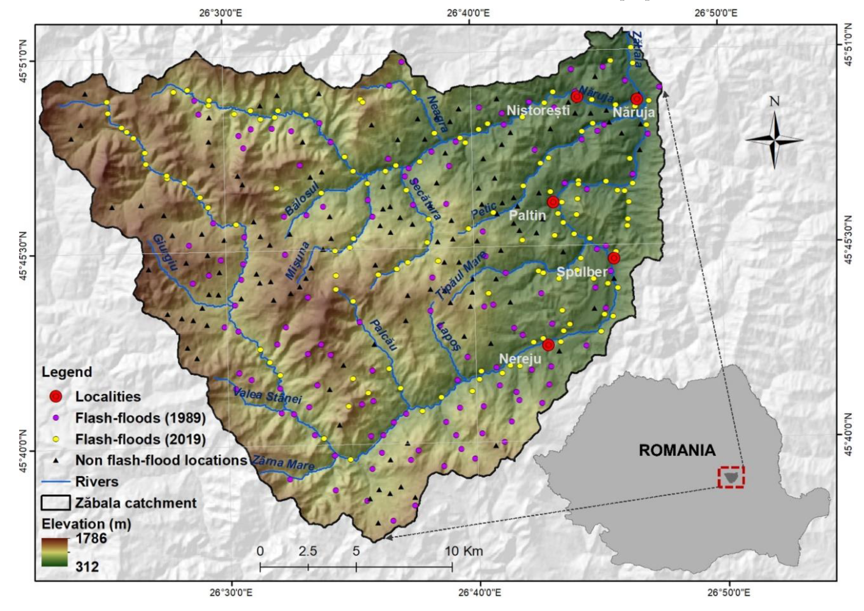
2. Study Area
3. Data and Methods
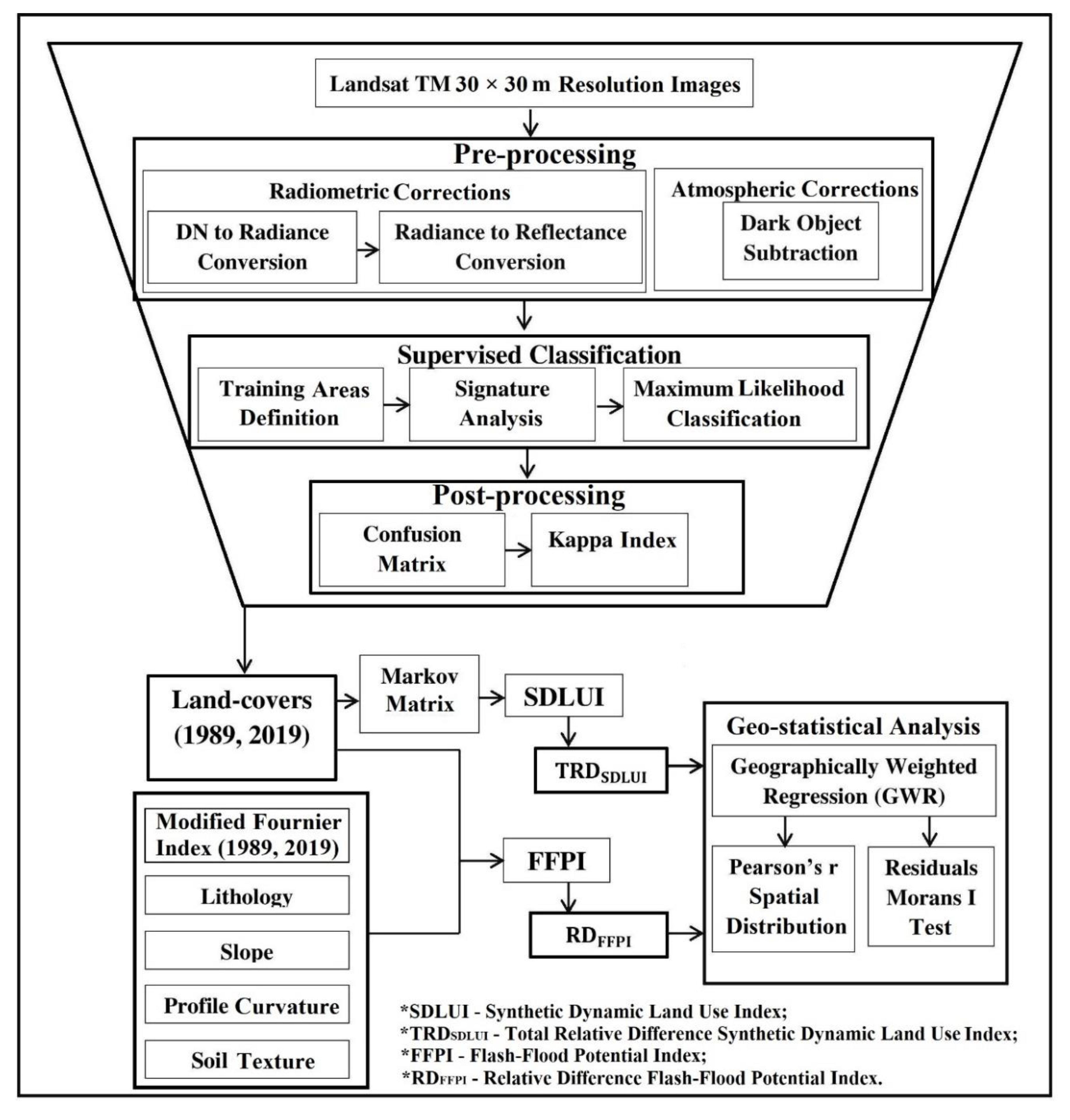
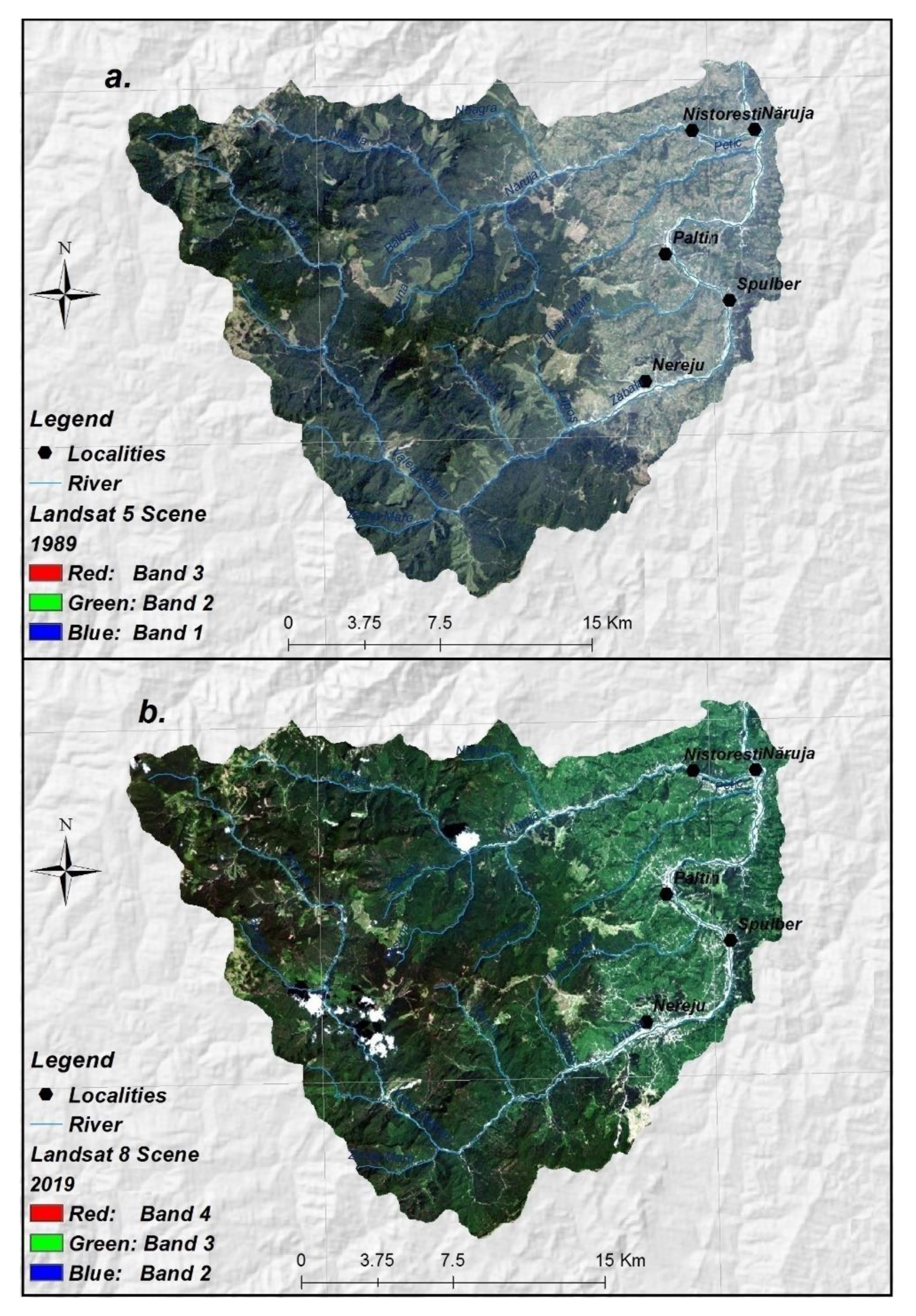
3.1. Remote Sensing Images Processing
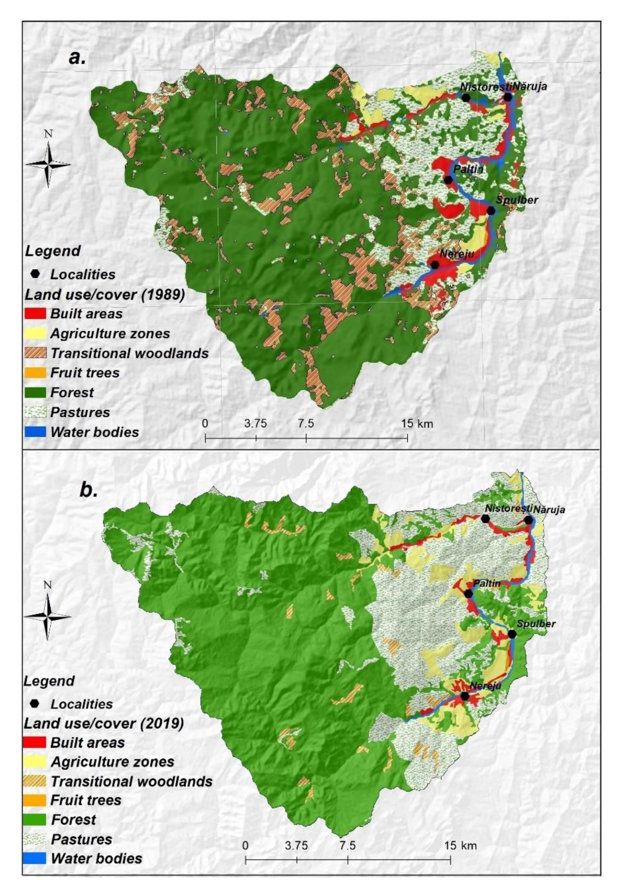
3.2. Land-Use/Land-Cover Change Analysis
3.3. Flash-Flood Potential Assessment
3.3.1. Flash-Flood Inventory
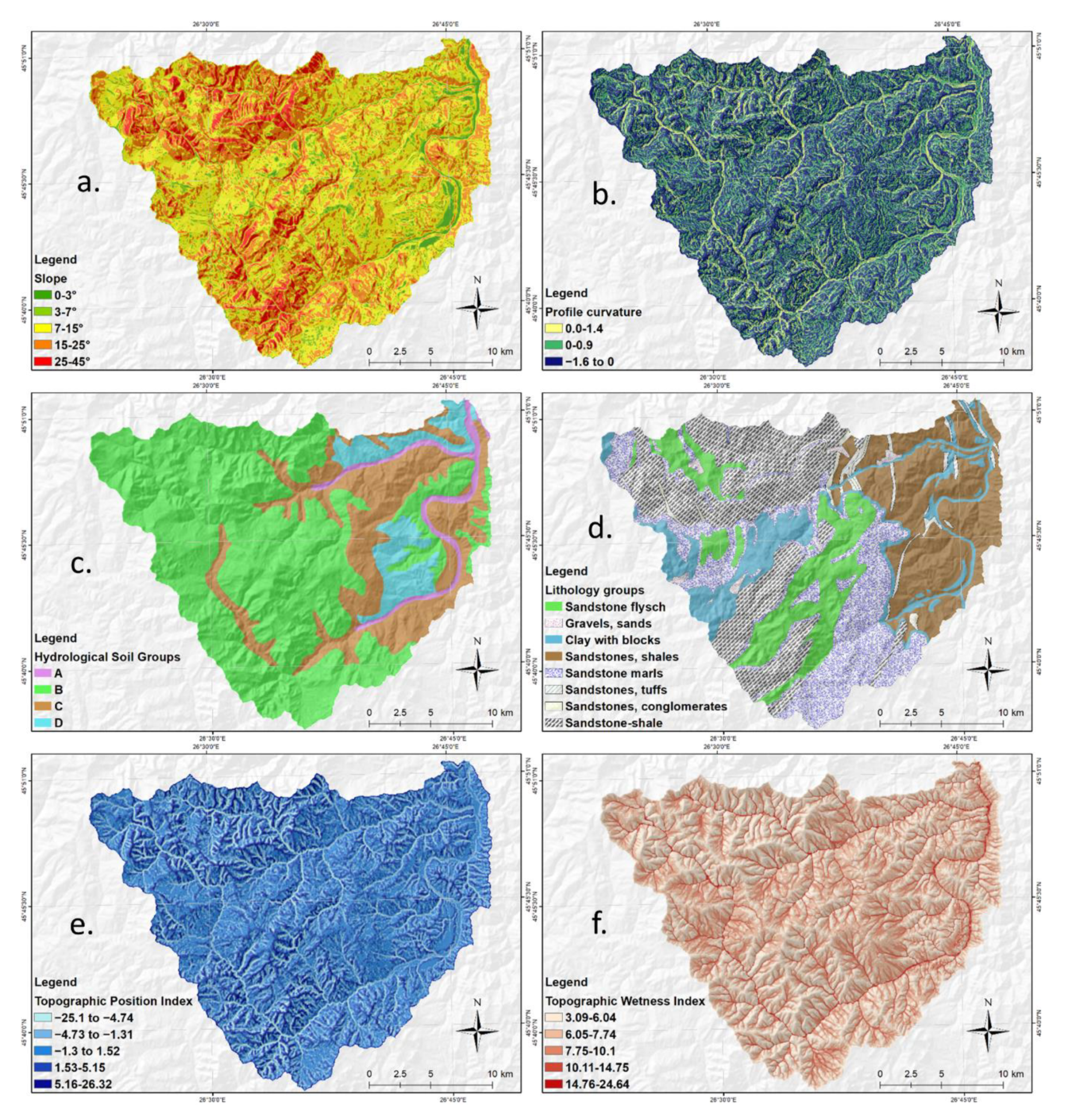
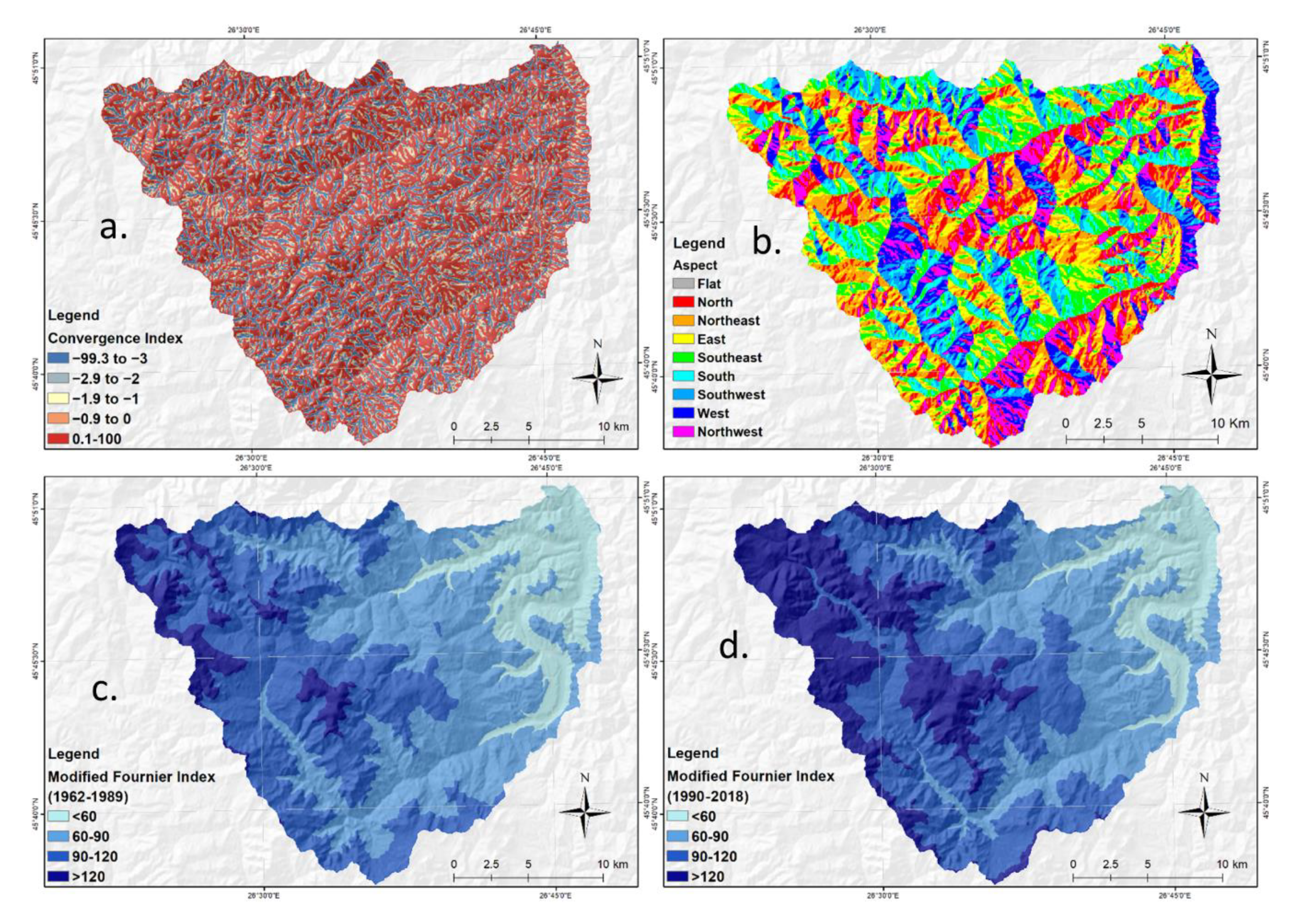
3.3.2. Flash-Flood Conditioning Factors
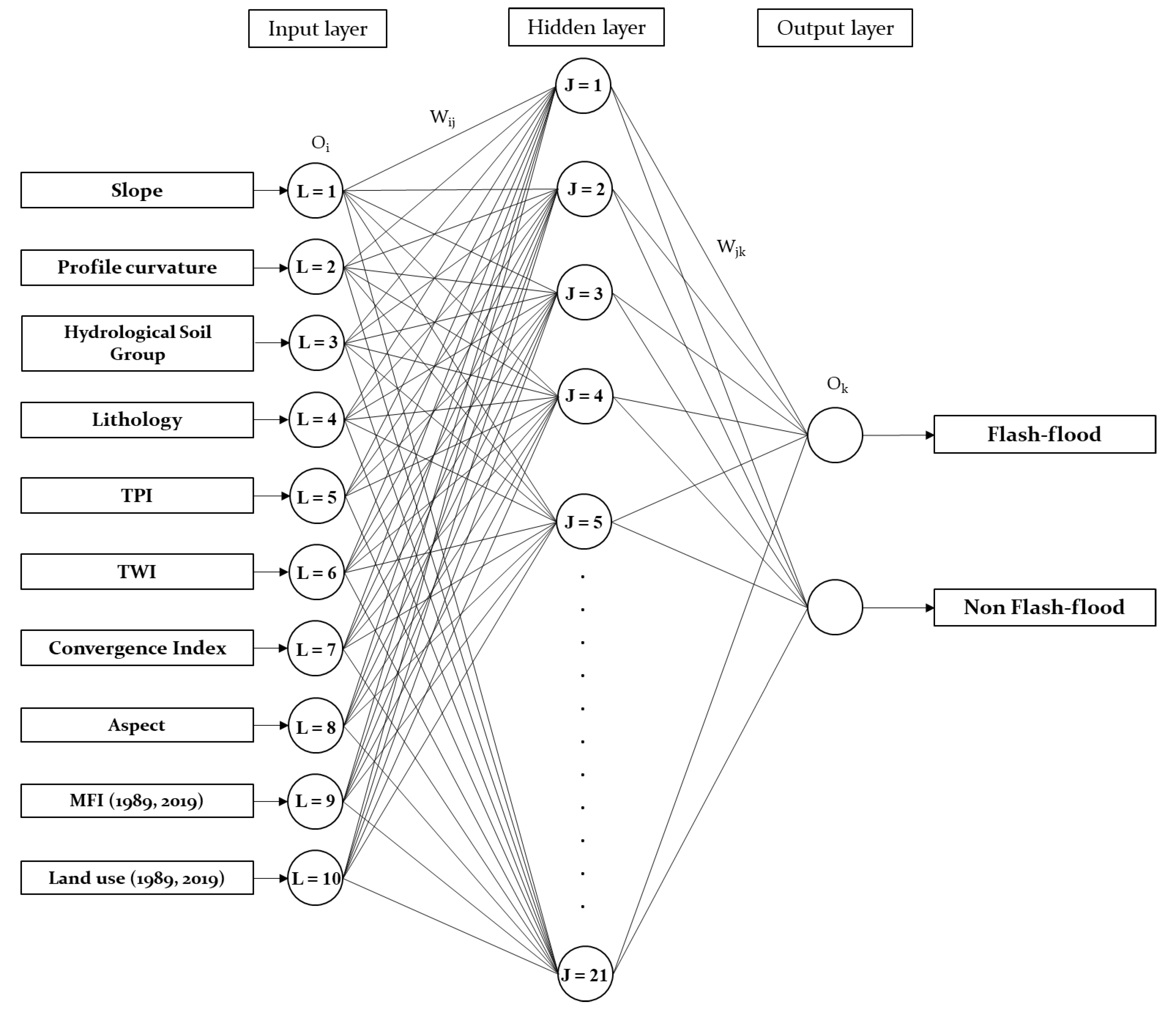
3.3.3. Description and Configuration of Multilayer Perceptron (MLP) Model for FFPI Computation
3.3.4. FFPI Results Validation
3.3.5. FFPI Differences
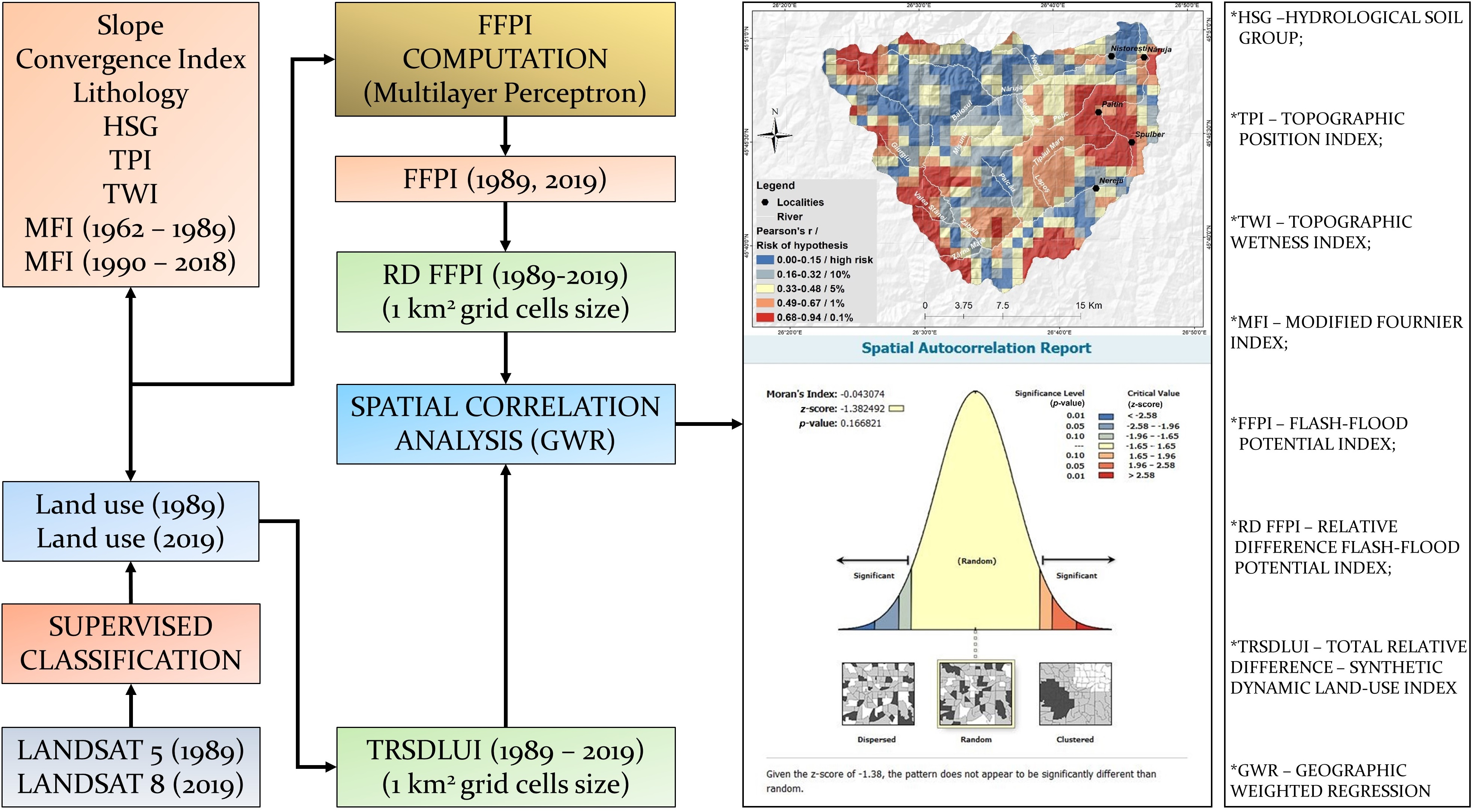
3.4. Geo-Statistical Analysis
4. Results
4.1. Results of the Imagery Classification
4.2. Result of Land-Use/Land-Cover Changes
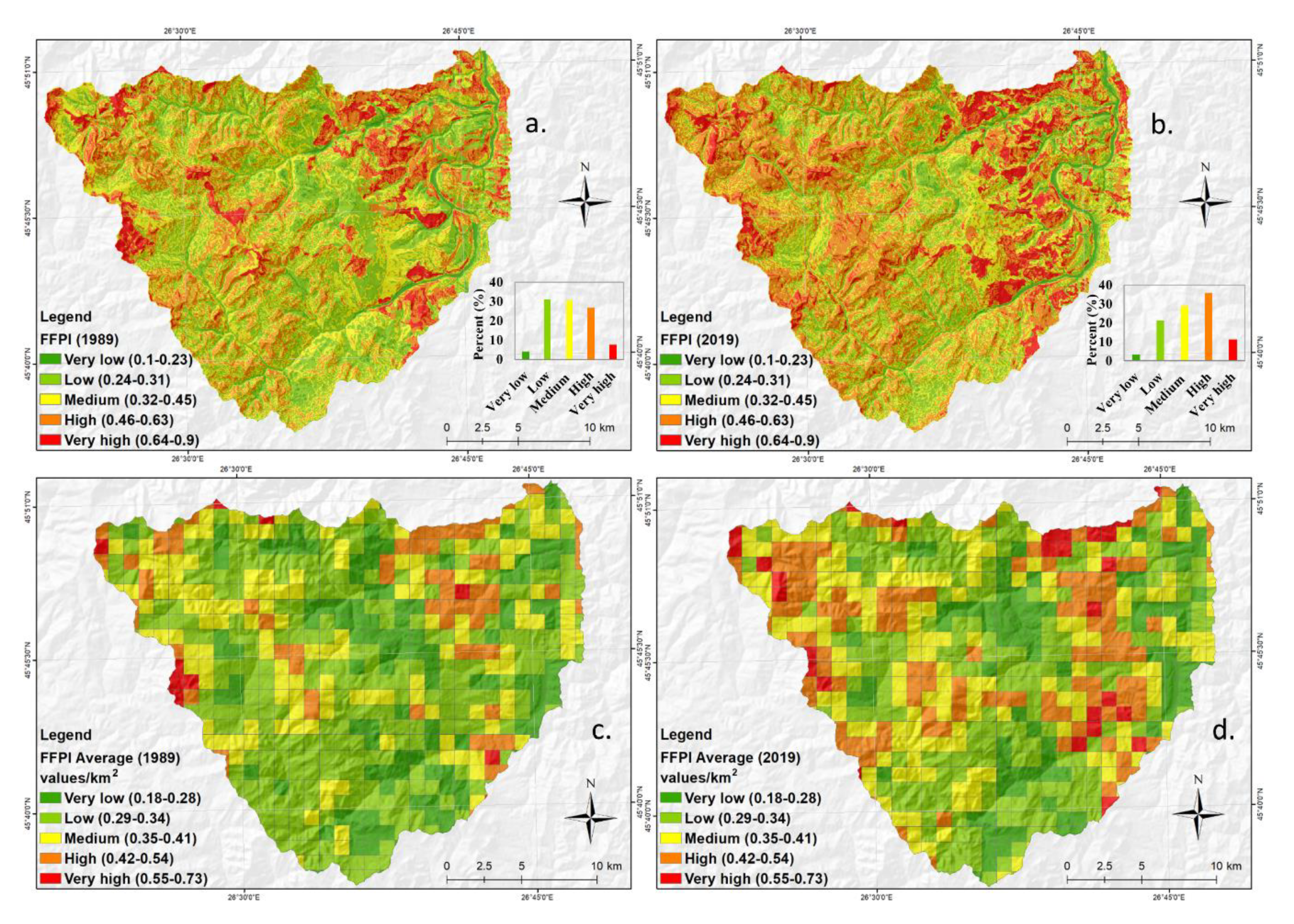
4.3. Run-off Risk Assessment (FFPI)
4.3.1. Flash-Flood Predictor Selection
4.3.2. Application of the MLP Model for FFPI Computation
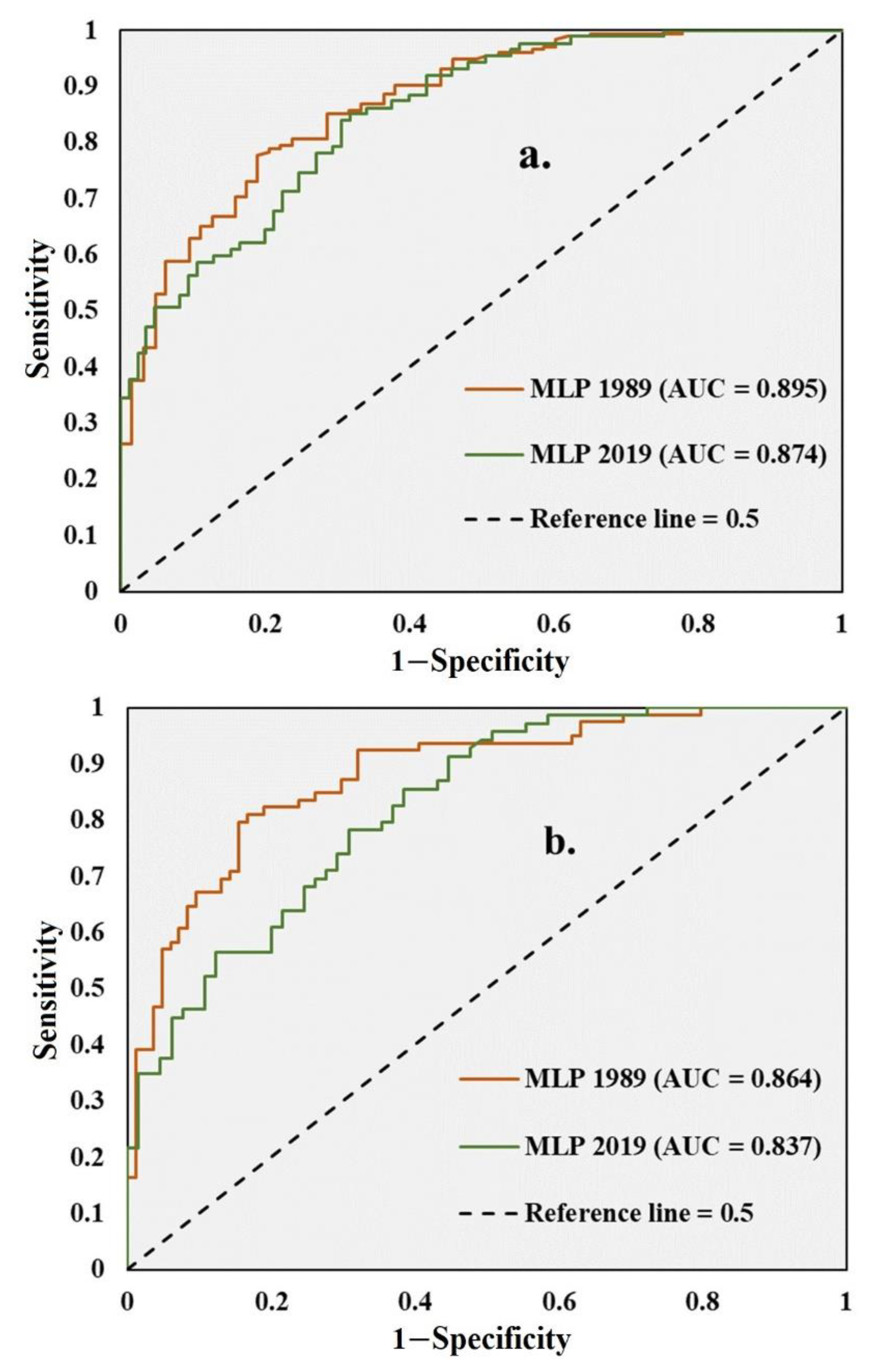
4.3.3. FFPI Results Validation
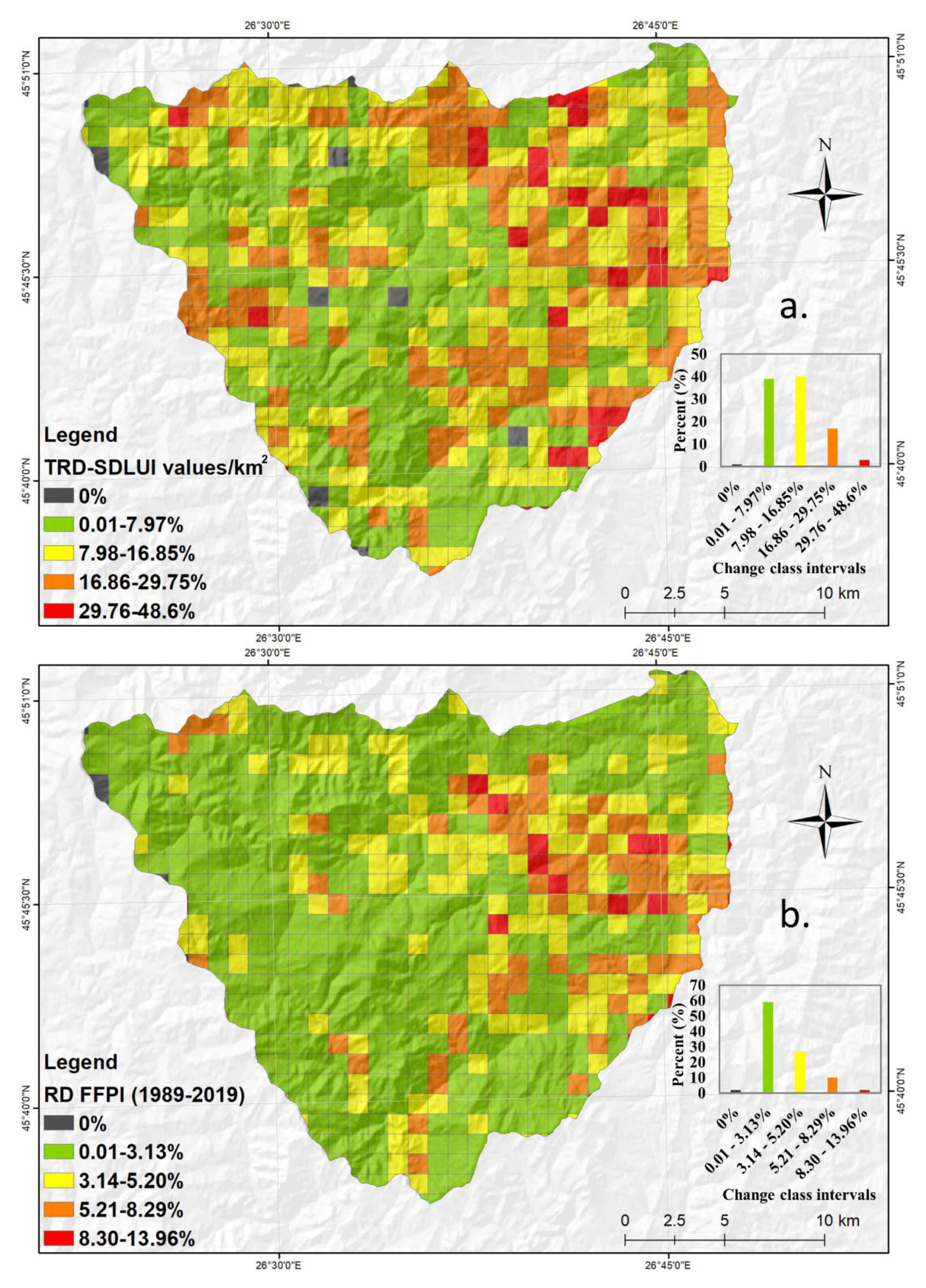
4.3.4. FFPI Differences
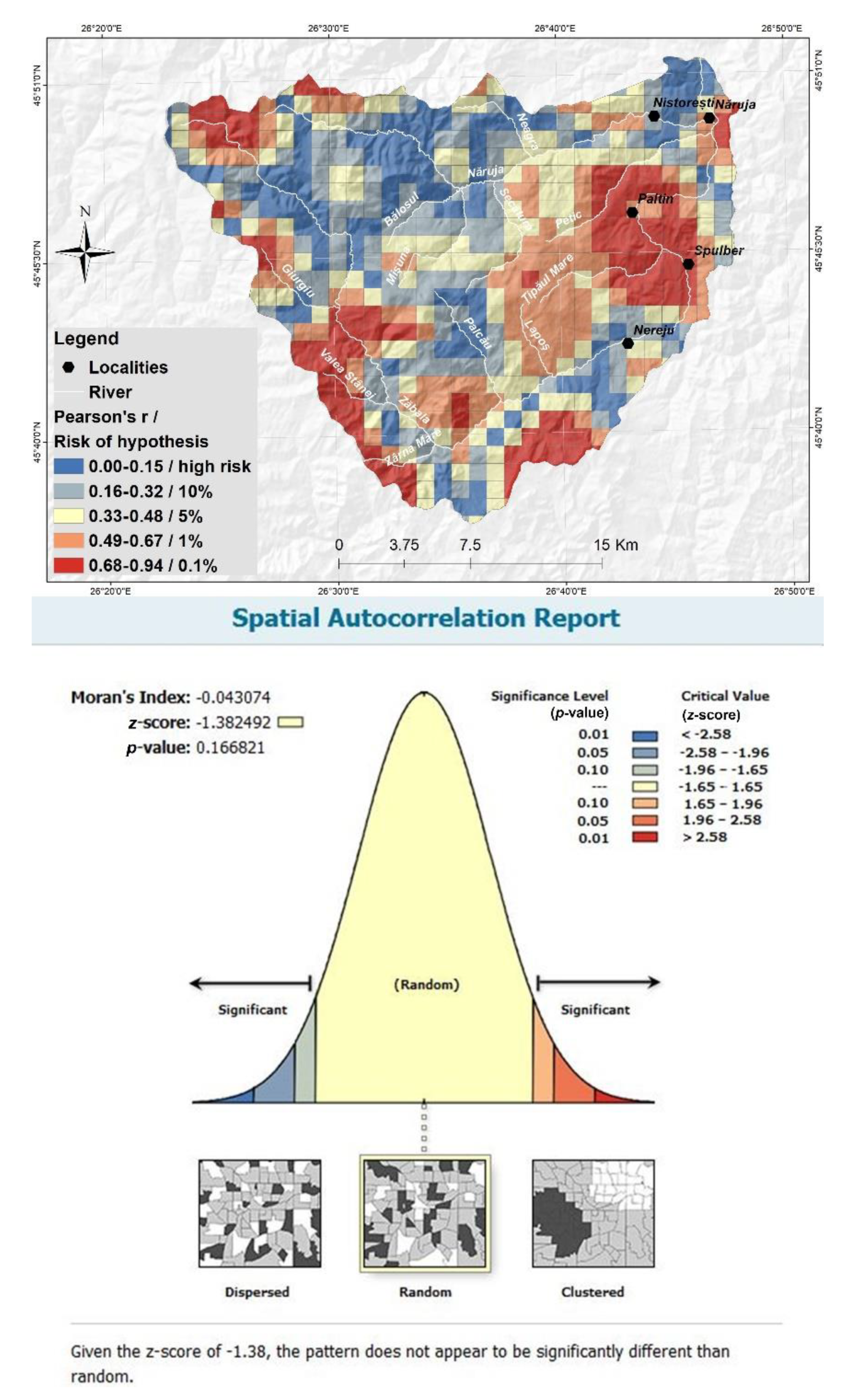
4.4. Statistical Analysis for Correlating and
5. Discussion
6. Conclusions
Author Contributions
Funding
Conflicts of Interest
References
- Arnell, N.W.; Gosling, S.N. The impacts of climate change on river flood risk at the global scale. Clim. Chang. 2016, 134, 387–401. [Google Scholar] [CrossRef] [Green Version]
- Bing, L.; Shao, Q.; Liu, J. Runoff characteristic in flood and dry seasons based on wavelet analysis in the source regions of Yangtze and Yellow River. In Proceedings of the International Conference on Remote Sensing, Environment and Transportation Engineering, Nanjing, China, 24–26 June 2011; pp. 705–710. [Google Scholar]
- Wang, S.; Yan, Y.; Yan, M.; Zhao, X. Quantitative estimation of the impact of precipitation and human activities on runoff change of the Huangfuchuan River Basin. J. Geogr. Sci. 2012, 22, 906–918. [Google Scholar] [CrossRef]
- Costea, G. Deforestation Process Consequences Upon Surface Runoff Coefficients. Catchment Level Case Study from the Apuseni Mountains, Romania. Geogr. Tech. 2013, 8, 28–33. [Google Scholar]
- Minea, G. Assessment of the flash flood potential of Bâsca River Catchment (Romania) based on physiographic factors. Open Geosci. 2013, 5, 344–353. [Google Scholar] [CrossRef] [Green Version]
- Cao, C.; Xu, P.; Wang, Y.; Chen, J.; Zheng, L.; Niu, C. Flash flood hazard susceptibility mapping using frequency ratio and statistical index methods in coalmine subsidence areas. Sustainability 2016, 8, 948. [Google Scholar] [CrossRef] [Green Version]
- Khosravi, K.; Pourghasemi, H.R.; Chapi, K.; Bahri, M. Flash flood susceptibility analysis and its mapping using different bivariate models in Iran: A comparison between Shannon’s entropy, statistical index, and weighting factor models. Environ. Monit. Assess. 2016, 188, 656. [Google Scholar] [CrossRef]
- Khosravi, K.; Pham, B.T.; Chapi, K.; Shirzadi, A.; Shahabi, H.; Revhaug, I.; Prakash, I.; Bui, D.T. A comparative assessment of decision trees algorithms for flash flood susceptibility modeling at Haraz watershed, northern Iran. Sci. Total Environ. 2018, 627, 744–755. [Google Scholar] [CrossRef]
- Bui, D.T.; Tsangaratos, P.; Ngo, P.-T.T.; Pham, T.D.; Pham, B.T. Flash flood susceptibility modeling using an optimized fuzzy rule based feature selection technique and tree based ensemble methods. Sci. Total Environ. 2019, 668, 1038–1054. [Google Scholar] [CrossRef]
- De Rosa, P.; Fredduzzi, A.; Cencetti, C. Stream Power Determination in GIS: An Index to Evaluate the Most ’Sensitive’ Points of a River. Water 2019, 11, 1145. [Google Scholar] [CrossRef] [Green Version]
- Borga, M.; Anagnostou, E.N.; Blöschl, G.; Creutin, J.D. Flash flood forecasting, warning and risk management: The HYDRATE project. Environ. Sci. Policy 2011, 14, 834–844. [Google Scholar] [CrossRef]
- Vojtek, M.; Vojteková, J. GIS-based Approach to Estimate Surface Runoff in Small Catchments: A Case Study. Quaest. Geogr. 2016, 35, 97–116. [Google Scholar] [CrossRef] [Green Version]
- Rogger, M.; Agnoletti, M.; Alaoui, A.; Bathurst, J.; Bodner, G.; Borga, M.; Chaplot, V.; Gallart, F.; Glatzel, G.; Hall, J. Land use change impacts on floods at the catchment scale: Challenges and opportunities for future research. Water Resour. Res. 2017, 53, 5209–5219. [Google Scholar] [CrossRef] [Green Version]
- Dang, A.T.N.; Kumar, L. Application of remote sensing and GIS-based hydrological modelling for flood risk analysis: A case study of District 8, Ho Chi Minh city, Vietnam. Geomat. Nat. Hazards Risk 2017, 8, 1792–1811. [Google Scholar] [CrossRef] [Green Version]
- Gan, B.; Liu, X.; Yang, X.; Wang, X.; Zhou, J. The impact of human activities on the occurrence of mountain flood hazards: Lessons from the 17 August 2015 flash flood/debris flow event in Xuyong County, south-western China. Geomat. Nat. Hazards Risk 2018, 9, 816–840. [Google Scholar] [CrossRef] [Green Version]
- Lieskovský, J.; Kaim, D.; Balázs, P.; Boltižiar, M.; Chmiel, M.; Grabska, E.; Király, G.; Konkoly-Gyuró, E.; Kozak, J.; Antalová, K.; et al. Historical land use dataset of the Carpathian region (1819–1980). J. Maps 2018, 14, 644–651. [Google Scholar] [CrossRef] [Green Version]
- Munteanu, C.; Kuemmerle, T.; Boltižiar, M.; Lieskovský, J.; Mojses, M.; Kaim, D.; Konkoly-Gyuro, E.; Mackovčin, P.; Müller, D.; Ostapowicz, K.; et al. Nineteenth-century land-use legacies affect contemporary land abandonment in the Carpathians. Reg. Environ. Chang. 2017, 11, 2209–2222. [Google Scholar] [CrossRef]
- Chen, Y.; Xu, Y.; Yin, Y. Impacts of land use change scenarios on storm-runoff generation in Xitiaoxi basin, China. Quat. Int. 2009, 208, 121–128. [Google Scholar] [CrossRef]
- Ali, M.; Khan, S.J.; Aslam, I.; Khan, Z. Simulation of the impacts of land-use change on surface runoff of Lai Nullah Basin in Islamabad, Pakistan. Landsc. Urban Plan. 2011, 102, 271–279. [Google Scholar] [CrossRef]
- Pielke, R.A.; Avissar, R. Influence of landscape structure on local and regional climate. Landsc. Ecol. 1990, 4, 133–155. [Google Scholar] [CrossRef]
- Chen, J.; Yu, Z.; Zhu, Y.; Yang, C. Relationship Between Land Use and Evapotranspiration—A Case Study of the Wudaogou Area in Huaihe River basin. Procedia Environ. Sci. 2011, 10, 491–498. [Google Scholar] [CrossRef] [Green Version]
- Mao, D.; Cherkauer, K.A. Impacts of land-use change on hydrologic responses in the Great Lakes region. J. Hydrol. 2009, 374, 71–82. [Google Scholar] [CrossRef]
- Khosravi, K.; Nohani, E.; Maroufinia, E.; Pourghasemi, H.R. A GIS-based flood susceptibility assessment and its mapping in Iran: A comparison between frequency ratio and weights-of-evidence bivariate statistical models with multi-criteria decision-making technique. Nat. Hazards 2016, 83, 947–987. [Google Scholar] [CrossRef]
- Elkhrachy, I. Flash Flood Hazard Mapping Using Satellite Images and GIS Tools: A case study of Najran City, Kingdom of Saudi Arabia (KSA). Egypt. J. Remote Sens. Space Sci. 2015, 18, 261–278. [Google Scholar] [CrossRef] [Green Version]
- Vojtek, M.; Vojteková, J. Flood Susceptibility Mapping on a National Scale in Slovakia Using the Analytical Hierarchy Process. Water 2019, 11, 364. [Google Scholar] [CrossRef] [Green Version]
- Dano, U.L.; Balogun, A.L.; Matori, A.N.; Yusouf, K.W.; Abubakar, I.R.; Mohamed, M.A.S.; Aina, Y.A.; Pradhan, B. Flood Susceptibility Mapping Using GIS-Based Analytic Network Process: A Case Study of Perlis, Malaysia. Water 2019, 11, 615. [Google Scholar] [CrossRef] [Green Version]
- Kourgialas, N.N.; Karatzas, G.P. Flood management and a GIS modelling method to assess flood-hazard areas–A case study. Hydrol. Sci. J. 2011, 56, 212–225. [Google Scholar] [CrossRef]
- Arabameri, A.; Rezaei, K.; Cerdà, A.; Conoscenti, C.; Kalantari, Z. A comparison of statistical methods and multi-criteria decision making to map flood Hazard susceptibility in Northern Iran. Sci. Total Environ. 2019, 660, 443–458. [Google Scholar] [CrossRef]
- Khosravi, K.; Shahabi, H.; Pham, B.T.; Adamowski, J.; Shirzadi, A.; Pradhan, B.; Dou, J.; Ly, H.B.; Gróf, G.; Ho, H.L.; et al. A comparative assessment of flood susceptibility modeling using Multi-Criteria Decision-Making Analysis and Machine Learning Methods. J. Hydrol. 2019, 573, 311–323. [Google Scholar] [CrossRef]
- Pradhan, B. Flood susceptible mapping and risk area delineation using logistic regression, GIS and remote sensing. J. Spat. Hydrol. 2010, 9, 1–18. [Google Scholar]
- Lee, S.; Lee, S.; Lee, M.J.; Jung, H.S. Spatial Assessment of Urban Flood Susceptibility Using Data Mining and Geographic Information System (GIS) Tools. Sustainability 2018, 10, 648. [Google Scholar] [CrossRef] [Green Version]
- Siahkamari, S.; Haghizadeh, A.; Zeinivand, H.; Tahmasebipour, N.; Rahmati, O. Spatial prediction of flood-susceptible areas using frequency ratio and maximum entropy models. Geocarto Int. 2018, 33, 927–941. [Google Scholar] [CrossRef]
- Bui, D.T.; Khosravi, K.; Shahabi, H.; Daggupati, P.; Adamowski, J.F.; Melesse, A.M.; Pham, B.T.; Pourghasemi, H.R.; Mahmoudi, M.; Bahrami, S.; et al. Flood Spatial Modeling in Northern Iran Using Remote Sensing and GIS: A Comparison between Evidential Belief Functions and Its Ensemble with a Multivariate Logistic Regression Model. Remote Sens. 2019, 11, 1589. [Google Scholar]
- Mosavi, A.; Ozturk, P.; Chau, K. Flood Prediction Using Machine Learning Models: Literature Review. Water 2018, 10, 1536. [Google Scholar] [CrossRef] [Green Version]
- Youssef, A.M.; Pradhan, B.; Hassan, A.M. Flash flood risk estimation along the St. Katherine road, southern Sinai, Egypt using GIS based morphometry and satellite imagery. Environ. Earth Sci. 2011, 62, 611–623. [Google Scholar] [CrossRef]
- Termeh, S.V.R.; Kornejady, A.; Pourghasemi, H.R.; Keesstra, S. Flood susceptibility mapping using novel ensembles of adaptive neuro fuzzy inference system and metaheuristic algorithms. Sci. Total Environ. 2018, 615, 438–451. [Google Scholar] [CrossRef]
- Lee, S.; Kim, J.C.; Jung, H.S.; Lee, M.J.; Lee, S. Spatial prediction of flood susceptibility using random-forest and boosted-tree models in Seoul metropolitan city, Korea. Geomat. Nat. Hazards Risk 2017, 8, 1185–1203. [Google Scholar] [CrossRef] [Green Version]
- Tehrany, M.S.; Pradhan, B.; Jebur, M.N. Flood susceptibility analysis and its verification using a novel ensemble support vector machine and frequency ratio method. Stoch. Environ. Res. Risk Assess. 2015, 29, 1149–1165. [Google Scholar] [CrossRef]
- Chapi, K.; Singh, V.P.; Shirzadi, A.; Shahabi, H.; Bui, D.T.; Pham, B.T.; Khosravi, K. A novel hybrid artificial intelligence approach for flood susceptibility assessment. Environ. Model. Softw. 2017, 95, 229–245. [Google Scholar] [CrossRef]
- Ahmadlou, M.; Karimi, M.; Alizadeh, S.; Shirzadi, A.; Parvinnejhad, D.; Shahabi, H.; Panah, M. Flood susceptibility assessment using integration of adaptive network-based fuzzy inference system (ANFIS) and biogeography-based optimization (BBO) and BAT algorithms (BA). Geocarto Int. 2019, 34, 1252–1272. [Google Scholar] [CrossRef]
- Choubin, B.; Moradi, E.; Golshan, M.; Adamowski, J.; Sajedi-Hosseini, F.; Mosavi, A. An ensemble prediction of flood susceptibility using multivariate discriminant analysis, classification and regression trees, and support vector machines. Sci. Total Environ. 2019, 651, 2087–2096. [Google Scholar] [CrossRef]
- Livni, R.; Shalev-Shwartz, S.; Shamir, O. On the computational efficiency of training neural networks. In Proceedings of the 27th International Conference on Neural Information Processing Systems, Montreal, QC, Canada, 8–13 December 2014; pp. 855–863. [Google Scholar]
- Heidari, A.A.; Faris, H.; Aljarah, I.; Mirjalili, S. An efficient hybrid multilayer perceptron neural network with grasshopper optimization. Soft Comput. 2019, 23, 7941–7958. [Google Scholar] [CrossRef]
- Pham, B.T.; Nguyen, M.D.; Bui, K.T.T.; Prakash, I.; Chap, K.; Bui, D.T. A novel artificial intelligence approach based on Multi-layer Perceptron Neural Network and Biogeography-based Optimization for predicting coefficient of consolidation of soil. Catena 2019, 173, 302–311. [Google Scholar] [CrossRef]
- Pham, B.T.; Tien Bui, D.; Prakash, I.; Dholakia, M.B. Hybrid integration of Multilayer Perceptron Neural Networks and machine learning ensembles for landslide susceptibility assessment at Himalayan area (India) using GIS. Catena 2017, 149, 52–63. [Google Scholar] [CrossRef]
- Xi, W.; Li, G.; Moayedi, H.; Nguyen, H. A particle-based optimization of artificial neural network for earthquake-induced landslide assessment in Ludian county, China. Geomat. Nat. Hazards Risk 2019, 10, 1750–1771. [Google Scholar] [CrossRef] [Green Version]
- Oh, H.J.; Syifa, M.; Lee, C.W.; Lee, S. Land Subsidence Susceptibility Mapping Using Bayesian, Functional, and Meta-Ensemble Machine Learning Models. Appl. Sci. 2019, 9, 1248. [Google Scholar] [CrossRef] [Green Version]
- Bui, D.T.; Nhu, V.H.; Hoan, N.D. Prediction of soil compression coefficient for urban housing project using novel integration machine learning approach of swarm intelligence and Multi-layer Perceptron Neural Network. Adv. Eng. Inf. 2018, 38, 593–604. [Google Scholar]
- Ngo, P.T.T.; Hoan, N.D.; Pradhan, B.; Nguyen, Q.K.; Tran, X.T.; Nguyen, Q.M.; Nguyen, V.N.; Samui, P.; Bui, D.T. A Novel Hybrid Swarm Optimized Multilayer Neural Network for Spatial Prediction of Flash Floods in Tropical Areas Using Sentinel-1 SAR Imagery and Geospatial Data. Sensors 2018, 18, 3704. [Google Scholar] [CrossRef] [Green Version]
- Bui, D.T.; Ngo, P.T.T.; Pham, T.D.; Jaafari, A.; Minh, N.Q.; Hoa, P.V.; Samui, P. A novel hybrid approach based on a swarm intelligence optimized extreme learning machine for flash flood susceptibility mapping. Catena 2019, 179, 184–196. [Google Scholar] [CrossRef]
- Jahangir, M.H.; Reineh, S.M.; Abolghasemi, M. Spatial predication of flood zonation mapping in Kan River Basin, Iran, using artificial neural network algorithm. Weather Clim. Extrem. 2019, 25, 100215. [Google Scholar] [CrossRef]
- Kia, M.B.; Pirasteh, S.; Pradhan, B.; Mahmud, A.R.; Sulaiman, W.N.A.; Moradi, A. An artificial neural network model for flood simulation using GIS: Johor River Basin, Malaysia. Environ. Earth Sci. 2012, 67, 251–264. [Google Scholar] [CrossRef]
- Zaharia, L.; Minea, G.; Ioana-Toroimac, G.; Barbu, R.; Sârbu, I. Estimation of the areas with accelerated surface runoff in the upper Prahova watershed (Romanian Carpathians). In Proceedings of the BALWOIS, Ohrid, Macedonia, 28 May–2 June 2012. [Google Scholar]
- Zaharia, L.; Costache, R.; Prăvălie, R.; Ioana-Toroimac, G. Mapping flood and flooding potential indices: A methodological approach to identifying areas susceptible to flood and flooding risk. Case study: The Prahova catchment (Romania). Front. Earth Sci. 2017, 11, 229–247. [Google Scholar] [CrossRef]
- General Inspectorate for Emergency Situations. The Archive of General Inspectorate for Emergency Situation—Vrancea County Subsidiary; General Inspectorate for Emergency Situations: Bucharest, Romania, 2019; Available online: http://www.isujvn.ro/ro-ro/ (accessed on 13 July 2019).
- Military Topographic Department. Topographic Map of Romania, 2nd ed.; (1:25,000); MApN, R.S.R.: Bucharest, Romania, 1982. Available online: https://www.geomil.ro/Produse/HartiTopografice (accessed on 16 July 2019).
- Arghiuş, C.; Arghiuş, V. The quantitative estimation of the soil erosion using USLE type ROMSEM model: Case-study-the Codrului ridge and Piedmont (Romania). Carpathian J. Earth Environ. Sci. 2011, 6, 59–66. [Google Scholar]
- Linzer, H.-G.; Frisch, W.; Zweigel, P.; Girbacea, R.; Hann, H.-P.; Moser, F. Kinematic evolution of the Romanian Carpathians. Tectonophysics 1998, 297, 133–156. [Google Scholar] [CrossRef]
- Singh, S.; Singh, C.; Mukherjee, S. Impact of land-use and land-cover change on groundwater quality in the Lower Shiwalik hills: A remote sensing and GIS based approach. Open Geosci. 2010, 2, 124–131. [Google Scholar] [CrossRef]
- Zhang, H.; Qi, Z.; Ye, X.; Cai, Y.; Ma, W.; Chen, M. Analysis of land use/land cover change, population shift, and their effects on spatiotemporal patterns of urban heat islands in metropolitan Shanghai, China. Appl. Geogr. 2013, 44, 121–133. [Google Scholar] [CrossRef]
- Liu, Z.; Liu, Y. Does Anthropogenic Land Use Change Play a Role in Changes of Precipitation Frequency and Intensity over the Loess Plateau of China? Remote Sens. 2018, 10, 1818. [Google Scholar] [CrossRef] [Green Version]
- Wang, J.; Zhang, W.; Zhang, Z. Impacts of Land-Use Changes on Soil Erosion in Water–Wind Crisscross Erosion Region of China. Remote Sens. 2019, 11, 1732. [Google Scholar] [CrossRef] [Green Version]
- Cloude, S.R.; Pottier, E. An entropy based classification scheme for land applications of polarimetric SAR. IEEE Trans. Geosci. Remote Sens. 1997, 35, 68–78. [Google Scholar] [CrossRef]
- Samaniego, L.; Bárdossy, A.; Schulz, K. Supervised classification of remotely sensed imagery using a modified k-NN technique. IEEE Trans. Geosci. Remote Sens. 2008, 46, 2112–2125. [Google Scholar] [CrossRef]
- Mather, P.; Tso, B. Classification Methods for Remotely Sensed Data; CRC Press: Boca Raton, FL, USA, 2016; ISBN 1-4200-9074-7. [Google Scholar]
- Zheng, B.; Myint, S.W.; Thenkabail, P.S.; Aggarwal, R.M. A support vector machine to identify irrigated crop types using time-series Landsat NDVI data. Int. J. Appl. Earth Obs. Geoinf. 2015, 34, 103–112. [Google Scholar] [CrossRef]
- Otukei, J.R.; Blaschke, T. Land cover change assessment using decision trees, support vector machines and maximum likelihood classification algorithms. Int. J. Appl. Earth Obs. Geoinf. 2010, 12, S27–S31. [Google Scholar] [CrossRef]
- Erbek, F.S.; Özkan, C.; Taberner, M. Comparison of maximum likelihood classification method with supervised artificial neural network algorithms for land use activities. Int. J. Remote Sens. 2004, 25, 1733–1748. [Google Scholar] [CrossRef]
- Karan, S.K.; Samadder, S.R. Accuracy of land use change detection using support vector machine and maximum likelihood techniques for open-cast coal mining areas. Environ. Monit. Assess. 2016, 188, 486. [Google Scholar] [CrossRef] [PubMed]
- Richards, J.A. Remote Sensing Digital Image Analysis; Springer: Berlin/Heidelberg, Germany, 1999. [Google Scholar]
- Du, Y.; Teillet, P.M.; Cihlar, J. Radiometric normalization of multitemporal high-resolution satellite images with quality control for land cover change detection. Remote Sens. Environ. 2002, 82, 123–134. [Google Scholar] [CrossRef]
- Lillesand, T.; Kiefer, R.W.; Chipman, J. Remote Sensing and Image Interpretation; John Wiley & Sons: Hoboken, NJ, USA, 2015; ISBN 1-118-34328-X. [Google Scholar]
- Ilori, C.O.; Pahlevan, N.; Knudby, A. Analyzing Performances of Different Atmospheric Correction Techniques for Landsat 8: Application for Coastal Remote Sensing. Remote Sens. 2019, 11, 469. [Google Scholar] [CrossRef] [Green Version]
- Reimann, J.; Schwerdt, M.; Schmidt, K.; Klenk, P.T.; Steinbrecher, U.; Breit, H. Precise Antenna Pointing Determination in Elevation for Spaceborne SAR Systems Using Coherent Pattern Differences. Remote Sens. 2019, 11, 320. [Google Scholar] [CrossRef] [Green Version]
- Rawat, J.; Kumar, M. Monitoring land use/cover change using remote sensing and GIS techniques: A case study of Hawalbagh block, district Almora, Uttarakhand, India. Egypt. J. Remote Sens. Space Sci. 2015, 18, 77–84. [Google Scholar] [CrossRef] [Green Version]
- Padró, J.-C.; Muñoz, F.-J.; Ávila, L.; Pesquer, L.; Pons, X. Radiometric correction of Landsat-8 and Sentinel-2A scenes using drone imagery in synergy with field spectroradiometry. Remote Sens. 2018, 10, 1687. [Google Scholar] [CrossRef] [Green Version]
- Coppin, P.; Jonckheere, I.; Nackaerts, K.; Muys, B.; Lambin, E. Digital change detection methods in ecosystem monitoring: A review. Int. J. Remote Sens. 2004, 25, 1565–1596. [Google Scholar] [CrossRef]
- Chavez, P.S. Image-based atmospheric corrections-revisited and improved. Photogramm. Eng. Remote Sens. 1996, 62, 1025–1035. [Google Scholar]
- Howarth, P.J.; Wickware, G.M. Procedures for change detection using Landsat digital data. Int. J. Remote Sens. 1981, 2, 277–291. [Google Scholar] [CrossRef]
- Petrişor, A.-I. Using CORINE data to look at deforestation in Romania: Distribution & possible consequences. Urban. Arhit. Construcţii 2015, 6, 83–90. [Google Scholar]
- Makantasis, K.; Karantzalos, K.; Doulamis, A.; Doulamis, N. Deep Supervised Learning for Hyperspectral Data Classification through Convolutional Neural Networks; IEEE: Piscataway, NJ, USA, 2015; pp. 4959–4962. [Google Scholar]
- Congalton, R.G.; Green, K. Assessing the Accuracy of Remotely Sensed Data: Principles and Practices, 2nd ed.; CRC Press: Boca Raton, FL, USA, 2019; ISBN 978-1-4987-7666-0. [Google Scholar]
- Eastman, J. Idrisi for Windows User’s Manual; Clark University: Worcester, MA, USA, 1995. [Google Scholar]
- Smith, G. Flash Flood Potential: Determining the Hydrologic Response of FFMP Basins to Heavy Rain by Analyzing Their Physiographic Characteristics. 2003. Available online: http://www.cbrfc.noaa.gov/papers/ffp_wpap.pdf (accessed on 8 August 2019).
- Kruzdlo, R.; Ceru, J. Flash Flood Potential Index for WFO Mount Holly/Philadelphia. 2010, pp. 2–4. Available online: http://bgmresearch.eas.cornell.edu/research/ERFFW/posters/kruzdlo_FlashFloodPotentialIndexforMountHollyHSA.pdf (accessed on 10 August 2019).
- Costache, R.; Bui, D.T. Spatial prediction of flood potential using new ensembles of bivariate statistics and artificial intelligence: A case study at the Putna river catchment of Romania. Sci. Total Environ. 2019, 691, 1098–1118. [Google Scholar] [CrossRef] [PubMed]
- Fontanine, I.; Costache, R. Using GIS techniques for surface runoff potential analysis in the Subcarpathian area between Buzãu and Slãnic rivers, in Romania. Cinq Cont. 2013, 3, 47–57. [Google Scholar]
- Pravalie, R.; Costache, R. The Analysis of the Susceptibility of the Flash-Floods’ Genesis in the Area of the Hydrographical Basin of Bāsca Chiojdului River/Analiza Susceptibilitatii Genezei Viiturilor īn Aria Bazinului Hidrografic al Rāului Bāsca Chiojdului; University of Craiova, Department of Geography: Craiova, Romania, 2014; Volume 13, pp. 39–49. [Google Scholar]
- Tehrany, M.S.; Pradhan, B.; Mansor, S.; Ahmad, N. Flood susceptibility assessment using GIS-based support vector machine model with different kernel types. Catena 2015, 125, 91–101. [Google Scholar] [CrossRef]
- Tehrany, M.S.; Pradhan, B.; Jebur, M.N. Flood susceptibility mapping using a novel ensemble weights-of-evidence and support vector machine models in GIS. J. Hydrol. 2014, 512, 332–343. [Google Scholar] [CrossRef]
- Stewart, D.; Canfield, E.; Hawkins, R. Curve number determination methods and uncertainty in hydrologic soil groups from semiarid watershed data. J. Hydrol. Eng. 2011, 17, 1180–1187. [Google Scholar] [CrossRef]
- Duulatov, E.; Chen, X.; Amanambu, A.C.; Ochege, F.U.; Orozbaev, R.; Issanova, G.; Omurakunova, G. Projected Rainfall Erosivity Over Central Asia Based on CMIP5 Climate Models. Water 2019, 11, 897. [Google Scholar] [CrossRef] [Green Version]
- Costache, R.; Hong, H.; Wang, Y. Identification of torrential valleys using GIS and a novel hybrid integration of artificial intelligence, machine learning and bivariate statistics. Catena 2019, 183, 104179. [Google Scholar] [CrossRef]
- Costache, R. Flood Susceptibility Assessment by Using Bivariate Statistics and Machine Learning Models-A Useful Tool for Flood Risk Management. Water Resour. Manag. 2019, 33, 3239–3256. [Google Scholar] [CrossRef]
- Costache, R.; Zaharia, L. Flash-flood potential assessment and mapping by integrating the weights-of-evidence and frequency ratio statistical methods in GIS environment—Case study: Bâsca Chiojdului River catchment (Romania). J. Earth Syst. Sci. 2017, 126, 59. [Google Scholar] [CrossRef]
- Anquetin, S.; Braud, I.; Vannier, O.; Viallet, P.; Boudevillain, B.; Creutin, J.-D.; Manus, C. Sensitivity of the hydrological response to the variability of rainfall fields and soils for the Gard 2002 flash-flood event. J. Hydrol. 2010, 394, 134–147. [Google Scholar] [CrossRef]
- Costache, R. Flash-flood Potential Index mapping using weights of evidence, decision Trees models and their novel hybrid integration. Stoch. Environ. Res. Risk Assess. 2019, 33, 1375–1402. [Google Scholar] [CrossRef]
- Wang, Y.; Hong, H.; Chen, W.; Li, S.; Panahi, M.; Khosravi, K.; Shirzadi, A.; Shahabi, H.; Panahi, S.; Costache, R. Flood susceptibility mapping in Dingnan County (China) using adaptive neuro-fuzzy inference system with biogeography based optimization and imperialistic competitive algorithm. J. Environ. Manag. 2019, 247, 712–729. [Google Scholar] [CrossRef] [PubMed]
- Zaharia, L.; Costache, R.; Prăvălie, R.; Minea, G. Assessment and mapping of flood potential in the Slănic catchment in Romania. J. Earth Syst. Sci. 2015, 124, 1311–1324. [Google Scholar] [CrossRef] [Green Version]
- Fathizad, H.; Hakimzadeh, M.A.; Shamsi, S.F.; Yaghobi, S. Watershed-level rainfall erosivity mapping using GIS-based geostatistical modeling. J. Earth Sci. Res. 2017, 5, 13–22. [Google Scholar] [CrossRef]
- Kilmer, J.; Rodríguez, R. Ordinary least squares regression is indicated for studies of allometry. J. Evol. Biol. 2017, 30, 4–12. [Google Scholar] [CrossRef]
- Seo, Y.; Kim, S.; Singh, V.P. Estimating spatial precipitation using regression kriging and artificial neural network residual kriging (RKNNRK) hybrid approach. Water Resour. Manag. 2015, 29, 2189–2204. [Google Scholar] [CrossRef]
- Domniţa, M. Runoff Modeling Using GIS. Application in Torrential Basins in the Apuseni Mountains; Risoprint Publisher: Cluj Napoca, Romania, 2012. [Google Scholar]
- Sheela, K.G.; Deepa, S. Neural network based hybrid computing model for wind speed prediction. Neurocomputing 2013, 122, 425–429. [Google Scholar] [CrossRef]
- Costache, R. Flash-Flood Potential assessment in the upper and middle sector of Prahova river catchment (Romania). A comparative approach between four hybrid models. Sci. Total Environ. 2019, 659, 1115–1134. [Google Scholar] [CrossRef]
- Fotheringham, A.S.; Brunsdon, C.; Charlton, M. Geographically Weighted Regression: The Analysis of Spatially Varying Relationships; John Wiley & Sons: Hoboken, NJ, USA, 2003. [Google Scholar]
- Akaike, H. Akaike, H. A new look at the statistical model identification. In Selected Papers of Hirotugu Akaike; Springer: Berlin/Heidelberg, Germany, 1974; pp. 215–222. [Google Scholar]
- Mitchell, A. The ESRI Guide to GIS Analysis; ESRI Press: Redlands, CA, USA, 2005; Volume 2. [Google Scholar]
- Li, H.; Calder, C.A.; Cressie, N. Beyond Moran’s I: Testing for spatial dependence based on the spatial autoregressive model. Geogr. Anal. 2007, 39, 357–375. [Google Scholar] [CrossRef]
- Pal, M.; Mather, P.M. Support vector machines for classification in remote sensing. Int. J. Remote Sens. 2005, 26, 1007–1011. [Google Scholar] [CrossRef]
- Asamoah, J.N.; Jnr, E.M.O.; Acquah, P.C.; Amoah, A.S. Comparison of Decision Tree and Maximum Likelihood Using a Landsat Image of Ejisu-Juaben Municipality. In Proceedings of the International Coference on Applied Sciences and Technology (ICAST), Kumasi, Ghana, 19 April 2018; Volume 4, pp. 200–210. [Google Scholar]
- Ali, M.Z.; Qazi, W.; Aslam, N. A comparative study of ALOS-2 PALSAR and Landsat-8 imagery for land cover classification using maximum likelihood classifier. Egypt. J. Remote Sens. Space Sci. 2018, 21, S29–S35. [Google Scholar] [CrossRef]
- Ajaj, Q.M.; Pradhan, B.; Noori, A.M.; Jebur, M.N. Spatial monitoring of desertification extent in western Iraq using Landsat images and GIS. Land Degrad. Dev. 2017, 28, 2418–2431. [Google Scholar] [CrossRef]
- Pham, B.T.; Jaafari, A.; Prakash, I.; Singh, S.K.; Quoc, N.K.; Bui, D.T. Hybrid computational intelligence models for groundwater potential mapping. Catena 2019, 182, 104101. [Google Scholar] [CrossRef]
- Tien Bui, D.; Shirzadi, A.; Chapi, K.; Shahabi, H.; Pradhan, B.; Pham, B.T.; Singh, V.P.; Chen, W.; Khosravi, K.; Bin Ahmad, B. A Hybrid Computational Intelligence Approach to Groundwater Spring Potential Mapping. Water 2019, 11, 2013. [Google Scholar] [CrossRef] [Green Version]
- Phong, T.V.; Phan, T.T.; Prakash, I.; Singh, S.K.; Shirzadi, A.; Chapi, K.; Ly, H.-B.; Ho, L.S.; Quoc, N.K.; Pham, B.T. Landslide susceptibility modeling using different artificial intelligence methods: A case study at Muong Lay district, Vietnam. Geocarto Int. 2019, 1–24. [Google Scholar] [CrossRef]
- Tien Bui, D.; Shirzadi, A.; Shahabi, H.; Geertsema, M.; Omidvar, E.; Clague, J.J.; Thai Pham, B.; Dou, J.; Talebpour Asl, D.; Bin Ahmad, B. New Ensemble Models for Shallow Landslide Susceptibility Modeling in a Semi-Arid Watershed. Forests 2019, 10, 743. [Google Scholar] [CrossRef] [Green Version]
- Chang, K.-T.; Merghadi, A.; Yunus, A.P.; Pham, B.T.; Dou, J. Evaluating scale effects of topographic variables in landslide susceptibility models using GIS-based machine learning techniques. Sci. Rep. 2019, 9, 1–21. [Google Scholar] [CrossRef] [Green Version]
- Termeh, S.V.R.; Khosravi, K.; Sartaj, M.; Keesstra, S.D.; Tsai, F.T.-C.; Dijksma, R.; Pham, B.T. Optimization of an adaptive neuro-fuzzy inference system for groundwater potential mapping. Hydrogeol. J. 2019, 1–24. [Google Scholar] [CrossRef]
- Nohani, E.; Moharrami, M.; Sharafi, S.; Khosravi, K.; Pradhan, B.; Pham, B.T.; Lee, S.; M Melesse, A. Landslide susceptibility mapping using different GIS-based bivariate models. Water 2019, 11, 1402. [Google Scholar] [CrossRef] [Green Version]
- Dou, J.; Yunus, A.P.; Xu, Y.; Zhu, Z.; Chen, C.-W.; Sahana, M.; Khosravi, K.; Yang, Y.; Pham, B.T. Torrential rainfall-triggered shallow landslide characteristics and susceptibility assessment using ensemble data-driven models in the Dongjiang Reservoir Watershed, China. Nat. Hazards 2019, 97, 579–609. [Google Scholar] [CrossRef]
- Wang, G.; Yang, H.; Wang, L.; Xu, Z.; Xue, B. Using the SWAT model to assess impacts of land use changes on runoff generation in headwaters. Hydrol. Process. 2014, 28, 1032–1042. [Google Scholar] [CrossRef]
- Anand, J.; Gosain, A.K.; Khosa, R. Prediction of land use changes based on Land Change Modeler and attribution of changes in the water balance of Ganga basin to land use change using the SWAT model. Sci. Total Environ. 2018, 644, 503–519. [Google Scholar] [CrossRef] [PubMed]
- Morán-Tejeda, E.; Zabalza, J.; Rahman, K.; Gago-Silva, A.; López-Moreno, J.I.; Vicente-Serrano, S.; Lehmann, A.; Tague, C.L.; Beniston, M. Hydrological impacts of climate and land-use changes in a mountain watershed: Uncertainty estimation based on model comparison. Ecohydrology 2015, 8, 1396–1416. [Google Scholar] [CrossRef]
- Worku, T.; Khare, D.; Tripathi, S. Modeling runoff–sediment response to land use/land cover changes using integrated GIS and SWAT model in the Beressa watershed. Environ. Earth Sci. 2017, 76, 550. [Google Scholar] [CrossRef]
- Gessesse, B.; Bewket, W.; Bräuning, A. Model-based characterization and monitoring of runoff and soil erosion in response to land use/land cover changes in the Modjo watershed, Ethiopia. Land Degrad. Dev. 2015, 26, 711–724. [Google Scholar] [CrossRef]
- Jodar-Abellan, A.; Valdes-Abellan, J.; Pla, C.; Gomariz-Castillo, F. Impact of land use changes on flash flood prediction using a sub-daily SWAT model in five Mediterranean ungauged watersheds (SE Spain). Sci. Total Environ. 2019, 657, 1578–1591. [Google Scholar] [CrossRef]
- Nilawar, A.P.; Waikar, M.L. Use of SWAT to determine the effects of climate and land use changes on streamflow and sediment concentration in the Purna River basin, India. Environ. Earth Sci. 2018, 77, 783. [Google Scholar] [CrossRef]
- Zuo, D.; Xu, Z.; Yao, W.; Jin, S.; Xiao, P.; Ran, D. Assessing the effects of changes in land use and climate on runoff and sediment yields from a watershed in the Loess Plateau of China. Sci. Total Environ. 2016, 544, 238–250. [Google Scholar] [CrossRef]


| Year. | Overall Acc. (%) | Kappa Index | Class | Ground Truth Samples (Pixels) | T.C. Pixels | User Acc. (%) | ||||||
|---|---|---|---|---|---|---|---|---|---|---|---|---|
| B.A. | A.Z. | F.T. | P. | F. | T.W. | W.B. | ||||||
| 1989 | 93.7 | 0.92 | B.A. | 347 | 0 | 2 | 0 | 2 | 0 | 7 | 358 | 96.9 |
| A.Z. | 3 | 179 | 1 | 3 | 3 | 4 | 3 | 196 | 91.3 | |||
| F.T. | 0 | 0 | 125 | 0 | 0 | 0 | 4 | 129 | 96.9 | |||
| P. | 1 | 4 | 1 | 271 | 18 | 7 | 6 | 308 | 88.0 | |||
| F. | 0 | 3 | 6 | 5 | 783 | 10 | 1 | 808 | 96.9 | |||
| T.W. | 0 | 0 | 0 | 0 | 29 | 252 | 0 | 281 | 89.7 | |||
| W.B. | 7 | 0 | 3 | 0 | 2 | 4 | 114 | 130 | 87.7 | |||
| T.G.T. Pixels | 358 | 186 | 138 | 279 | 837 | 277 | 135 | 2210 | ||||
| Prod. Acc. (%) | 96.9 | 96.2 | 90.6 | 97.1 | 93.5 | 91.0 | 84.4 | |||||
| 2019 | 95.23 | 0.939 | B.A. | 419 | 0 | 0 | 0 | 1 | 0 | 6 | 426 | 98.4 |
| A.Z. | 2 | 245 | 7 | 0 | 0 | 0 | 0 | 254 | 96.5 | |||
| F.T. | 0 | 2 | 56 | 0 | 0 | 0 | 0 | 58 | 96.6 | |||
| P. | 10 | 0 | 0 | 173 | 9 | 0 | 6 | 198 | 87.4 | |||
| F. | 0 | 5 | 1 | 7 | 706 | 25 | 8 | 752 | 93.9 | |||
| T.W. | 2 | 0 | 0 | 7 | 0 | 229 | 0 | 238 | 96.2 | |||
| W.B. | 2 | 0 | 0 | 0 | 0 | 0 | 172 | 174 | 98.9 | |||
| T.G.T. Pixels | 435 | 252 | 64 | 187 | 716 | 254 | 192 | 2100 | ||||
| Prod. Acc. (%) | 96.3 | 97.2 | 87.5 | 92.5 | 98.6 | 90.2 | 90.2 | |||||
| 1989\2019 | Agricultural Areas | Transitional Woodland | Built-Up Areas | Forests | Pastures | Water Bodies | Fruit Trees | Losses (ha) |
|---|---|---|---|---|---|---|---|---|
| Agricultural areas | - | 2.91 | 12.06 | 55.92 | 318.61 | 0 | 0 | 389.5 |
| Transitional woodland | 21.99 | - | 2.62 | 1554.83 | 97.87 | 0.27 | 12.43 | 1677.58 |
| Built-up areas | 564.13 | 0 | - | 34.39 | 3293.4 | 17.49 | 42.42 | 3909.41 |
| Forests | 53.73 | 4088.73 | 104.8 | - | 4088.73 | 23.3 | 0 | 8359.29 |
| Pastures | 906.6 | 666.66 | 220.01 | 1090.5 | - | 16.91 | 100.32 | 3000.9 |
| Water bodies | 7.45 | 16.58 | 51.37 | 48.75 | 32.91 | - | 0 | 157.06 |
| Fruit trees | 0 | 4.51 | 12.54 | 0 | 4.23 | 0 | - | 21.28 |
| Gain (ha) | 1553.9 | 4779.39 | 403.4 | 2784.39 | 7835.75 | 57.97 | 155.17 | 17,569.97 |
| Flood Predictor | AM1989 | AM2019 |
|---|---|---|
| Slope | 0.87 | 0.91 |
| TPI | 0.28 | 0.39 |
| TWI | 0.61 | 0.46 |
| Land use/land cover | 0.47 | 0.73 |
| Lithology | 0.52 | 0.59 |
| Profile curvature | 0.41 | 0.22 |
| Aspect | 0.17 | 0.13 |
| Convergence index | 0.35 | 0.32 |
| Hydrological soil groups | 0.23 | 0.26 |
| MFI | 0.68 | 0.55 |
| Factor | Class | FR1989 | FR1989 N | FR2019 | FR2019 N | MLP1989 Weight | MLP2019 Weight |
|---|---|---|---|---|---|---|---|
| Slope | 0–3° | 0.00 | 0.10 | 0.33 | 0.20 | 0.373 | 0.404 |
| 3–7° | 0.20 | 0.18 | 0.00 | 0.10 | |||
| 7–15° | 0.43 | 0.27 | 0.25 | 0.17 | |||
| 15–25° | 1.98 | 0.90 | 1.93 | 0.67 | |||
| 25–45° | 1.20 | 0.58 | 2.72 | 0.90 | |||
| TPI | −25.1 to −4.74 | 1.47 | 0.90 | 1.35 | 0.90 | 0.097 | 0.103 |
| −4.73 to −1.31 | 0.93 | 0.33 | 1.21 | 0.75 | |||
| −1.3 to 1.52 | 1.01 | 0.41 | 1.03 | 0.56 | |||
| 1.53–5.15 | 0.98 | 0.38 | 0.70 | 0.21 | |||
| 5.16–26.32 | 0.72 | 0.10 | 0.60 | 0.10 | |||
| TWI | 3.09–6.04 | 1.27 | 0.90 | 1.14 | 0.66 | 0.104 | 0.194 |
| 6.05–7.74 | 1.13 | 0.81 | 1.09 | 0.64 | |||
| 7.75–10.1 | 0.14 | 0.10 | 0.37 | 0.28 | |||
| 10.11–14.75 | 0.90 | 0.64 | 1.62 | 0.90 | |||
| 14.76–24.64 | 0.67 | 0.48 | 0.00 | 0.10 | |||
| Land use/land cover | Built-up areas | 2.13 | 0.59 | 2.21 | 0.56 | 0.287 | 0.236 |
| Agriculture zone | 0.28 | 0.15 | 1.01 | 0.29 | |||
| Shrub | 2.21 | 0.60 | 3.16 | 0.78 | |||
| Fruit trees | 3.46 | 0.90 | 2.58 | 0.65 | |||
| Forests | 0.08 | 0.10 | 0.16 | 0.10 | |||
| Pastures | 0.64 | 0.23 | 0.37 | 0.15 | |||
| Water bodies | 2.45 | 0.66 | 3.70 | 0.90 | |||
| Lithology | Sandstone flysch | 0.91 | 0.65 | 0.58 | 0.17 | 0.146 | 0.128 |
| Gravels, sands | 0.00 | 0.10 | 1.02 | 0.30 | |||
| Clay with blocks | 0.90 | 0.64 | 0.79 | 0.23 | |||
| Sandstone, shales | 1.12 | 0.77 | 1.54 | 0.46 | |||
| Sandstone, marls | 0.47 | 0.38 | 2.79 | 0.84 | |||
| Sandstone, tuffs | 0.70 | 0.52 | 2.79 | 0.84 | |||
| Sandstone, conglomerates | 1.09 | 0.75 | 3.00 | 0.90 | |||
| Sandstone-shale | 1.34 | 0.90 | 0.35 | 0.10 | |||
| Profile curvature | 0.9–1.4 | 1.52 | 0.90 | 1.79 | 0.90 | 0.059 | 0.045 |
| 0–0.9 | 0.86 | 0.10 | 1.11 | 0.40 | |||
| −1.6 to 0 | 0.99 | 0.26 | 0.71 | 0.10 | |||
| Aspect | Flat surfaces | 0.00 | 0.10 | 0.00 | 0.10 | 0.051 | 0.032 |
| North | 0.98 | 0.63 | 1.09 | 0.86 | |||
| North-East | 1.32 | 0.81 | 1.12 | 0.88 | |||
| East | 1.25 | 0.77 | 0.92 | 0.74 | |||
| South-East | 0.72 | 0.49 | 0.72 | 0.60 | |||
| South | 0.79 | 0.53 | 1.15 | 0.90 | |||
| South-West | 0.67 | 0.46 | 1.00 | 0.80 | |||
| West | 0.56 | 0.40 | 0.96 | 0.77 | |||
| North-East | 1.48 | 0.90 | 1.06 | 0.84 | |||
| Convergence index | −99.3 to −3 | 0.76 | 0.10 | 0.40 | 0.14 | 0.05 | 0.084 |
| −3 to −2 | 0.79 | 0.16 | 0.34 | 0.10 | |||
| −2 to −1 | 1.13 | 0.90 | 1.04 | 0.54 | |||
| −1–0 | 1.10 | 0.85 | 1.61 | 0.90 | |||
| 0–100 | 1.09 | 0.82 | 1.21 | 0.65 | |||
| (Hydrological Soil Group (HSG) | A | 1.70 | 0.67 | 1.70 | 0.10 | 0.043 | 0.067 |
| B | 0.70 | 0.10 | 1.90 | 0.29 | |||
| C | 1.51 | 0.57 | 2.10 | 0.47 | |||
| D | 2.10 | 0.90 | 2.56 | 0.90 | |||
| MFI | <60 | 1.01 | 0.10 | 1.34 | 0.10 | 0.122 | 0.289 |
| 60–90 | 1.24 | 0.43 | 1.52 | 0.52 | |||
| 90–120 | 1.56 | 0.90 | 1.68 | 0.90 | |||
| >120 | 1.32 | 0.55 | 1.48 | 0.43 |
© 2019 by the authors. Licensee MDPI, Basel, Switzerland. This article is an open access article distributed under the terms and conditions of the Creative Commons Attribution (CC BY) license (http://creativecommons.org/licenses/by/4.0/).
Share and Cite
Costache, R.; Bao Pham, Q.; Corodescu-Roșca, E.; Cîmpianu, C.; Hong, H.; Thi Thuy Linh, N.; Ming Fai, C.; Najah Ahmed, A.; Vojtek, M.; Muhammed Pandhiani, S.; et al. Using GIS, Remote Sensing, and Machine Learning to Highlight the Correlation between the Land-Use/Land-Cover Changes and Flash-Flood Potential. Remote Sens. 2020, 12, 1422. https://0-doi-org.brum.beds.ac.uk/10.3390/rs12091422
Costache R, Bao Pham Q, Corodescu-Roșca E, Cîmpianu C, Hong H, Thi Thuy Linh N, Ming Fai C, Najah Ahmed A, Vojtek M, Muhammed Pandhiani S, et al. Using GIS, Remote Sensing, and Machine Learning to Highlight the Correlation between the Land-Use/Land-Cover Changes and Flash-Flood Potential. Remote Sensing. 2020; 12(9):1422. https://0-doi-org.brum.beds.ac.uk/10.3390/rs12091422
Chicago/Turabian StyleCostache, Romulus, Quoc Bao Pham, Ema Corodescu-Roșca, Cătălin Cîmpianu, Haoyuan Hong, Nguyen Thi Thuy Linh, Chow Ming Fai, Ali Najah Ahmed, Matej Vojtek, Siraj Muhammed Pandhiani, and et al. 2020. "Using GIS, Remote Sensing, and Machine Learning to Highlight the Correlation between the Land-Use/Land-Cover Changes and Flash-Flood Potential" Remote Sensing 12, no. 9: 1422. https://0-doi-org.brum.beds.ac.uk/10.3390/rs12091422