Detection, Segmentation, and Model Fitting of Individual Tree Stems from Airborne Laser Scanning of Forests Using Deep Learning


Australian Centre for Field Robotics, University of Sydney, Sydney NSW 2006, Australia
*
Author to whom correspondence should be addressed.
†
Current address: Australian Centre for Field Robotics, University of Sydney, Sydney NSW 2006, Australia.
Remote Sens. 2020, 12(9), 1469; https://0-doi-org.brum.beds.ac.uk/10.3390/rs12091469
Submission received: 9 April 2020
/
Revised: 26 April 2020
/
Accepted: 30 April 2020
/
Published: 6 May 2020
(This article belongs to the Special Issue 3D Point Clouds in Forest Remote Sensing)
Abstract
:Accurate measurements of the structural characteristics of trees such as height, diameter, sweep and taper are an important part of forest inventories in managed forests and commercial plantations. Both terrestrial and aerial LiDAR are currently employed to produce pointcloud data from which inventory metrics can be determined. Terrestrial/ground-based scanning typically provides pointclouds resolutions of many thousands of points per m from which tree stems can be observed and inventory measurements made directly, whereas typical resolutions from aerial scanning (tens of points per m) require inventory metrics to be regressed from LiDAR variables using inventory reference data collected from the ground. Recent developments in miniaturised LiDAR sensors are enabling aerial capture of pointclouds from low-flying aircraft at high-resolutions (hundreds of points per m) from which tree stem information starts to become directly visible, enabling the possibility for plot-scale inventories that do not require access to the ground. In this paper, we develop new approaches to automated tree detection, segmentation and stem reconstruction using algorithms based on deep supervised machine learning which are designed for use with aerially acquired high-resolution LiDAR pointclouds. Our approach is able to isolate individual trees, determine tree stem points and further build a segmented model of the main tree stem that encompasses tree height, diameter, taper, and sweep. Through the use of deep learning models, our approach is able to adapt to variations in pointcloud densities and partial occlusions that are particularly prevalent when data is captured from the air. We present results of our algorithms using high-resolution LiDAR pointclouds captured from a helicopter over two Radiata pine forests in NSW, Australia.
1. Introduction
Accurate inventories of forests are an important part of effective forest management in regards to assessing the potential value of managed commercial plantations, assessing potential for fire hazards and monitoring for pests and disease [1]. Important metrics for forest inventories include structural metrics such as tree height, Diameter at Breast Height (DBH), stem basal area and volume, and stem form such as taper and sweep. Traditionally, these properties are measured at an individual tree level in large-scale sampling plots using fieldwork/manual measurements from the ground [2]. With the advent of Terrestrial Laser Scanning (TLS) sensors and systems, inventory metrics and other related structural attributes of trees can be captured and automatically processed in the field [3,4,5,6,7,8,9,10,11,12,13]. TLS produces LiDAR pointcloud densities of many thousands of points per m which can be used to directly measure tree stems; automated processes can then be developed to segment stem points and fit circular or cylindrical models, which are then used to extract tree-level structural metrics.
For inventories over large areas of forest, forests in remote areas or otherwise difficult or dangerous areas to access via the ground, surveys and inventories must be performed by aerial means. Airborne Laser Scanning (ALS) involves similar principles of operation as for TLS, but where the scanner is mounted to a high-flying aircraft, producing pointclouds with much lower densities. Most past work on ALS for forest inventories focused on methods in which inventory metrics are regressed from pointcloud information [14,15,16,17,18,19,20], rather than from directly measured individual tree stems, owing to the lower resolution and typical lack of direct stem measurements. These methods rely on a sample of field-based measurements of inventory metrics to build regression models that can work with low resolution pointclouds. More recently, miniturised high-resolution LiDAR systems (e.g., [21]) are enabling the capture of pointcloud densities from low-flying aircraft that are capable of measuring the structure and shape of tree stems directly (i.e., dense ALS, with densities of hundreds of points per m), but still at a much lower density and coverage than TLS. The ability to directly measure tree stem properties relevant for inventories from dense ALS would enable the opportunity for accurate aerial inventory that does not rely on ground-based measurements, which has the potential to increase the areal coverage, efficiency and safety of inventory activities.
In this paper, we develop new methods for the detection of individual trees, segmentation of stem points, and reconstruction of stem geometry (i.e., radius, sweep, taper) using dense aerial LiDAR pointclouds. Unlike TLS, where stems are often directly observed across the whole length and circumferential coverage of each tree [22], dense aerial pointclouds still contain many sections of missing points on stems in both the horizontal and vertical directions, owing to occlusions that occur when scanning from the air and through the forest canopy. Our algorithms can adapt to missing data and variations in point resolutions owing to the nature of aerial scanning by exploiting an approach built around deep learning on 3D pointclouds. 3D pointcloud learning is an emerging research area [22,23,24], driven by applications such as self-driving cars [25,26,27,28] remote sensing, airborne LiDAR and forestry [13]. The geometric models that are extracted for individual trees from our method can be used to directly measure forest inventory metrics (e.g., stocking, volume, DBH, etc.) thus enabling the potential for aerial forest inventory without the need for information collected from the ground.
1.1. Related Work
Many valuable structural metrics usually cannot be directly measured from ALS data due to factors such as scanning angle, insufficient point density and the canopy obstructing pulses from stems. Instead, methods typically determine how variables that can be accurately derived from ALS (e.g., canopy height) are empirically related to structural metrics measured in the field. To find correlations and model this dependence, methods fit linear models [14,15], use non-parametric regression [16,17] and copulas [29] among other techniques. Structural metrics are estimated at the stand-level using area-based approaches [18,19,20] or at the tree-level using either individual tree detection [16,17,29] or multisource single-tree inventory (MS-STI) techniques [30,31]. There is typically a trade-off where simple methods generalise well but perform poorly at extreme cases where the trees of interest differ significantly to those measured in the field, and vice versa for complex methods.
More recently, aerial methods for forest inventory moved towards detecting and delineating individual trees. Individual tree detection from low resolution ALS is usually accomplished by using the 3D structure of the canopy. Methods can be broadly grouped into several categories, with the most common approach involving detecting tree crowns as local maxima in a canopy height model (CHM), which is a 2D raster where the cell values represent the height of the canopy and other vegetation above the ground. Once trees are detected, tree points are delineated using algorithms such as marker-based watershed [32,33,34] or seeded region-growing [14,35], where the markers or seeds which guide the delineations are the tree detections. Other methods include clustering [36,37], morphological operations on 2D projections of the 3D data [38], graph-based methods [39,40] and a range of other techniques [41,42,43,44,45]. Tree detection allows for inventory metrics such as tree count, density and position maps to be inferred.
TLS is able to sense trees beneath the canopy, from the ground. Because there is no obstruction by the canopy, the stem of a tree can be measured directly from the data, which is usually captured with a much higher resolution than ALS due to its proximity to the target [3,4,5,6,7,8,9,10,11,12,13]. Rather then find correlations with LiDAR variables, methods are usually built around automatically segmenting the stem and/or fitting models (e.g., circular, cylindrical) to it, which are then used to extract tree-level structural metrics. These methods work well because the stem is accurately reconstructed in the data—hence the structural metrics can be extracted with more precision than the statistical estimation approaches typically used with ALS data. However, TLS is not as practical as ALS for estimating large forest inventories as it has a much smaller feasible area coverage, and requires ground-based access/fieldwork, which may be difficult in remote areas, rugged terrain or in forests with significant undergrowth. As such, TLS finds applications in automatically extracting structural metrics from smaller sample plots as well as developing and updating allometric models non-destructively [46].
There have been advances in the processing of high resolution 3D pointcloud data made in the fields of computer vision and robotics, driven by the demand for it in applications such as self-driving cars. Deep learning algorithms including Voxnet [22] and Shapenet [23] where filters convolve in 3D, pointnet [24] and its extensions [47,48] where networks are trained directly on points, and Voxelnet [49] which incorporates both of the former, were used for tasks such as object detection, classification and segmentation in pointcloud data. For self-driving car applications, robust algorithms were designed to process LiDAR pointcloud data captured in challenging, unstructured outdoor environments [25,26,27,28]. With the ability to collect high resolution ALS data, it is possible to draw from the advancements of recent work in these fields, and adapt them for application to forestry. The field of remote sensing progressively adopted deep learning techniques. They were used to process data collected from satellite imagery [50,51,52], hyperspectral imagery [53,54] and LiDAR [55,56,57]. Deep learning methods were incorporated into LiDAR forestry methods in recent work, most prominently in TLS applications where the point densities are high. Tree species classification was performed using pointclouds that were converted from 3D data to other forms, such as waveforms [58], 2D projections [59] and depth images [60]. Very recently, tree stems were labelled in TLS data using 3D-CNNs in Xi et al. [13]. Hamraz et al. apply a 2D-CNN to a 2D representation of the ALS data to classify whether a tree is coniferous or deciduous [61] and Ayrey and Hayes use a 3D-CNN to map voxelised ALS plots to forest metrics (above ground biomass, tree count and percent needleleaf) at the plot level [62].
1.2. Contributions of This Work
In previous work, the authors developed an approach to detecting trees and segmenting tree points using a combination of a region-based CNN object detection framework and a 3D-CNN using a voxelised pointcloud representation [21]. Our current work builds on and extends the work in this paper by developing and evaluating new data representations and deep learning architectures, comparing these to traditional, non-machine learning approaches, and evaluating results with additional annotations from the multiple dense aerial pointcloud datasets. We also develop a new algorithm for stem reconstruction via non-linear least squares model fitting to complete a unified pipeline for individual tree detection and delineation, stem segmentation and stem model fitting, which can be used to estimate tree-level structural attributes that are valuable for foresters.
The specific contributions of our paper are:
- A tree detection approach proposed in previous work [21] is extended by adding a new representations for the encoding of 3D pointcloud data into 2D rasterised summaries for detection. Evaluations are carried out with multiple aerial datasets.
- A stem segmentation approach proposed in previous work [21] is extended by incorporating voxel representations that include LiDAR return intensity into the learning representation, and we develop a new point-based deep learning architecture (based on Pointnet [24]), for tree pointcloud segmentation. Evaluations are carried out with multiple aerial datasets and different segmentation architectures are compared.
- We develop a new stem reconstruction technique using RANdom SAmple Concensus (RANSAC) and non-linear least squares that fits a flexible geometric model of a tree’s main stem to segmented stem points to compute the tree centreline position and stem radius at multiple points along the length of the stem. This model can then be used to extract inventory metrics such as height, diameters etc.
2. Materials
2.1. Study Areas
Pointcloud data was acquired from a Riegl VUX-1 LiDAR scanner attached to a helicopter flying over commercial pine plantation forests at Tumut, NSW, Australia (collected in November 2016) and Carabost, NSW, Australia (collected in February, 2018). Both forests were composed primarily of 23 year old (Carabost) and 26 year old (Tumut) Pinus radiata species, with stocking densities of 400 (Tumut) and 600 (Carabost) stems per hectare. The topography at each site was relatively flat with sparse patches of undergrowth approximately 1–2 m high, and slightly higher at the Carabost site.
2.2. Data Collection
During the LiDAR acquisitions, the helicopter flew approximately 60–90 m from the ground, resulting in a pointcloud density of approximately 300–700 points per m, a resolution much higher than conventional ALS collected from higher flying manned aircraft (typically 5–80 points per m), but still less than conventional TLS, which may provide scans of many thousands of points per m. The resulting datasets exhibit LiDAR hits on tree stems, but with frequent sections of missing hits along stems, due to occlusions in the data and a high degree of ‘clutter’ points from the surrounding forest canopy and undergrowth.
3. Methods
The aim of this approach is to locate individual trees in an ALS pointcloud and estimate their structural attributes, such as diameter at breast height (DBH), crown width, tree height and stem volume. To accomplish this, a multi-stage pipeline comprising ground characterisation and removal, delineation of individual trees, segmentation of tree points into stem and foliage and model fitting to stem points is proposed. The structural attributes of each tree can be inferred from its fitted model.
3.1. Overview
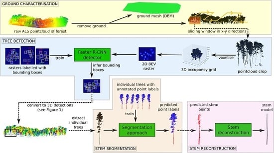
A high-level overview of the proposed pipeline is given in Figure 1. From the high resolution ALS data acquired over a forest, the ground is characterised with a digital terrain model (DTM) and ground points are removed from the pointcloud. Then, individual trees are detected and their tree points are delineated, allowing for the inference of attributes such as a stem map, tree counts and plot density, as well tree-level structural metrics such as crown width and tree height. Next, stem points are segmented from the pointclouds for individual trees, after which a model-fitting process fits small cylinders to the segmented stem points of each detected tree (i.e., stem reconstruction). From these cylinders, structural metrics such as the DBH, stem profile and stem volume can be obtained for each tree. A graphical overview of the pipeline is shown in Figure 2.
3.2. Ground Characterisation and Removal
Many of the ALS pulses received are returns from the ground. These points are important for the characterisation of the ground with a DTM, which in itself is a useful component for inventory. The DTM can be used for estimating attributes such as tree height. It is also necessary to know which points are returns from the ground so that they can be removed from the pointcloud. This simplifies the subsequent detection, segmentation and reconstruction steps. The method used in this paper produces a relatively coarse DTM. If a finer resolution is required (e.g., for precise measurement of tree height), than another tool should be used, such as points2grid (https://opentopography.org/otsoftware/points2grid) from Open Topography or Simple Morphological Filter (https://pdal.io/) from the PDAL library.
To build a DTM for the ground, the entire pointcloud is discretised into metre bins in the xy-plane. The point (x,y,z coordinate) in each bin with the smallest height is stored. Next, a grid with metre cells that spans the size of the pointcloud is created. A K-D Tree [63] is used to find the closest four points (in terms of euclidean distance in the xy-plane) from the subset stored previously to the centre location of each grid cell. The average of these four points, weighted by their distance to the grid cell centre, is calculated as the ground height for the given xy location in the grid. The height of each grid cell is computed in this way and then meshed using a delauney triangulation [64], which outputs a smooth DTM.
Once the DTM has been estimated, ground points can be removed by discarding all points within a height threshold above the DTM (which varies along the xy-plane). This threshold should be adjusted for different tasks. For example, it is useful to set it to two metres when doing tree detection, as this removes many of the points that belong to ground-based vegetation which can register as false positive trees. However, when doing the stem segmentation and reconstruction, the threshold should be lower because the DBH is usually measured at around 1.3 m (although a stem model can still be fit without these points). In the experiments, a threshold of 2 m is used for tree detection and 1 m for stem segmentation.
3.3. Individual Tree Detection
Once the ground points are removed from the pointcloud, individual trees are detected as subsets of points (i.e., trees are delineated). The task of delineation is more difficult than simply detecting tree crowns, but it allows for the extraction of inventory metrics such crown width and is necessary for stem segmentation. In this work, delineation is accomplished using a common approach to object detection in pointclouds [25,26] whereby a 2D, 3-channel image is generated from a birds-eye view projection (BEV) (i.e., projected into the xy-plane, see Figure 3) of the pointcloud for a Faster R-CNN object detector [65]—an approach designed for 2D imagery, to make bounding box detections on. Individual trees are delineated by projecting the 2D bounding box detections (Figure 4a) from the xy-plane into 3D cuboids that in-case the points belonging to each tree (Figure 4b).
The BEV Faster R-CNN approach to object detection has primarily found uses in vehicle perception applications [25,26]. However, there are reasons to justify its application in forestry, mainly that trees are reasonably uniform across a forest, with vertical cylindrical shapes that project conveniently into the BEV image without too much occlusion. The effectiveness of BEV rasters as a representation of ALS forest data was investigated in [66,67]. However, these methods use simpler approaches to delineating trees in the raster (e.g., watershed).
3.3.1. Individual Tree Detection: BEV Representations
The BEV is a three-channel image that encodes the 3D information in the pointcloud. In vehicle perception tasks, the BEV channels comprise vertical density, maximum height and average return and are obtained by discretising the pointcloud into voxels [25,26]. The vertical density is computed by summing the number of occupied voxels in the z axis for each grid location and dividing by the total number of occupied and un-occupied voxels. The max height is computed as the z-location of the highest occupied cell for each grid location. The average return is found by taking the mean of the return values of all points in all grids along the z-axis for each grid location.
This work explores the effectiveness of the BEV representation for tree detection by testing two different representations. The first representation is the vertical density converted to a three-channel colour image, encoding information about the density of points in the vertical axis—similar to the tree detection method proposed in Windrim et al. 2019 [21]. Trees have a characteristic appearance in this representation as their stems contribute to a high density circular shape near the centre of the lower density surrounding foliage. In this work, the grid size was m with a resolution of 0.2 m. This produces a 2D matrix, which is mapped to a 3-channel colour image using a ‘jet’ colour scale, producing a colour image. The second representation concatenates the vertical density, maximum height and average returns to make a three-channel image. An example of the two different BEV representations of the same plot is shown in Figure 3.
3.3.2. Individual Tree Detection: Training
To train the object detector, several 3D crops from the ground-removed pointcloud (with sizes less than m in x and y respectively, to fit within the grid with 0.2 m resolution) are converted to BEV images. The trees in each image are annotated with axis-aligned bounding boxes. Shrub and partial tree background classes are also annotated to reduce the number of false positives tree detections. The partial tree class contains trees which lie on the crop boundary. The BEV images with their bounding box labels are used to train a Faster-RCNN object detector. The Faster-RCNN network with a Resnet-101 backend [68] was trained for 10,000 iterations using Stochastic Gradient Descent (with momentum), a learning rate of 0.003, momentum of 0.9 and batch size of 1. The network was initialised with weights from training on the MS COCO dataset [69].
3.3.3. Individual Tree Detection: Inference
For inference, a window slides in the -plane of the ground-removed pointcloud and at each location the points whose x and y values are contained within the bounds of the window are cropped out and converted to a BEV. Trees, shrubs and partial trees in the BEV are detected with bounding boxes and class names using the trained Faster-RCNN model. Shrub and partial tree bounding boxes are discarded. Please note that the window slides with an overlap such that partial trees will appear as full trees in another window. Bounding boxes for all trees across the pointcloud are accumulated together and their coordinates are changed from local BEV coordinates to locations in the larger pointcloud. Finally, the 2D bounding boxes are projected into 3D cuboids such that all points whose x and y coordinates fall within the bounding box are detected as trees. The result is a set of points associated with each tree in the pointcloud.
3.4. Stem Segmentation
Once each individual tree has been detected as a set of 3D points, the points can be further segmented into stem and foliage components. For this, two deep learning approaches to pointcloud segmentation are tested. The first uses a voxel representation, where the set of points for a given tree are converted to a 3D occupancy grid and a 3D convolutional architecture is used to infer a semantic label for each voxel, which are converted back to points. The second approach, called pointnet, uses the raw point representation of the data to train a neural network to infer labels.
To train the segmentation networks, individual tree pointclouds were manually labelled using the CloudCompare software tool [70]. For each tree, points were labelled as either crown vegetation (referred to as foliage from this point in the manuscript, collectively referencing branches, twigs and leaves), stem or clutter class (clutter being anything other then stem or foliage, such as ground vegetation).
3.4.1. Stem Segmentation: 3D-FCN Architecture for Voxel Segmentation
The voxel approach for tree segmentation, shown in Figure 5a, draws from two seminal works in volumetric deep learning. The first is VoxNet [22], a 3D-CNN architecture for classification of LiDAR scans of object captured in urban environments (e.g., cars, pedestrians, bicyles). The second approach is V-net [71], which is a 3D fully convolutional encoder-decoder neural network (3D-FCN) designed for segmentation of 3D medical imagery (e.g., an MRI). The network designed for tree segmentation in this work adopts the 3D-FCN structure of V-net, but with similar convolutional layers (which are mirrored in the deconvolutional layers) to VoxNet.
For input, the network with architecture given in Figure 6a takes an occupancy grid for each tree of size voxels with resolution m in the x, y and z axes respectively. Two types of occupancy grid are experimented with: a binary type (Figure 7a) with only ones and zeros indicating occupancy and unknown occupancy/free space, and a non-binary type (Figure 7b) which instead has a pulse return value for each occupied voxel in the grid (and zeros for unknown occupancy/free space). The binary type is similar to the stem segmentation method proposed in Windrim et al. 2019 [21]. The network, comprising an encoder and decoder, is trained to reconstruct target semantic grids consisting of one binary occupancy grid for each of the three classes—empty space, foliage and stem (see Figure 5a). To adapt a ’one-hot’ style representation for the target labels, for each set of corresponding voxels across the three output grids, only one voxel is occupied (with a one) such that each voxel only has one class label. For locations with no points, the free space grid voxels will be occupied with a one. Points labelled as clutter are represented as occupied cells in the input, but in the output they occupy the empty space grid. This is to train the network to remove clutter from its output. As seen in Figure 6a, the network contains five fully convolutional layers, two of which are deconvolutional in the decoder. There are skip connections between corresponding encoder and decoder layers to preserve the resolution of the voxels when upsampling (i.e., deconvolving).
To train the voxel networks, the three occupancy grids output by the network are treated in a similar fashion to one-hot vectors for classification: a softmax non-linearity is applied across corresponding cells before a cross-entropy loss function compares predictions to the labelled target occupancy grids. The networks are trained with batches of individual tree pointclouds. Each batch of pointclouds—the input and labelled target, are converted to their occupancy grid representations on the fly. This is so that the batch can be augmented with random rotations and flipping about the z-axis, which must occur on the pointcloud before voxelisation. All voxel networks are trained from scratch. Networks are trained until convergence, with a learning rate of 0.001 which is decayed to 0.0001 after 500 iterations. The Adam optimiser is used [72], and classes are balanced at each batch by weighting their contributions to the total loss. The batch size and data augmentation is dependant on the total number of training samples and constrained by the GPU memory (11 GB). The batch size is six trees with four additional augmentations for each sample (30 trees per batch in total).
For inference, pointcloud crops detected as trees using the methodology of Section 3.3 are converted to binary occupancy grids (i.e., voxels) and passed through the trained voxel network. The network produces three binary occupancy grids (one for each class), which are converted to a labelled 3D pointcloud. The resultant pointcloud is usually of a lower resolution due to the downsampling of the voxelisation process. To recover the original resolution, a K-D Tree is built from the low resolution labelled point cloud that is output by the network and points from the original, high resolution pointcloud are used to query the K-D Tree in order to find the closest labelled point (within a thresholded distance). The result is a high resolution labelled pointcloud for the tree. Ideally there are no clutter points output in the low resolution pointcloud, so the clutter points in the original, high resolution pointcloud will exceed the distance threshold and have no label.
3.4.2. Stem Segmentation: Pointnet Architecture for Point Segmentation
Unlike the voxel architecture, the pointnet architecture uses a point-based representation of the data to train the network (Figure 5b). The approach taken in this work is based on the popular Pointnet [24] architecture, which is a style of neural network designed for points and is flexible enough to be used for both classification and segmentation. In this work, it is used to map the points for individual trees to foliage, stem and clutter class labels (i.e., segmentation).
The architecture used (Figure 6b) is similar to that of [24], but without the T-net components due to the rotational symmetry about the z-axis. Also, for computational efficiency, the MLP layers are implemented as 2D CNNs. Similar to the voxel architecture, two types of network are developed, one with points simply represented with x, y and z elements, and one with x, y, z and LiDAR pulse return. The latter has a similar architecture to Figure 6b, but with an input size of to incorporate the return intensity. Thus, the filters in the first layer are of size instead of . The architecture for both styles of network constitutes a global feature, which is obtained by pooling over the axis which spans the n points, and is replicated and appended to one of the lower level feature representations before several more layers of features are learnt. The network outputs a score for each of the three classes, for all points.
To train the network, the scores are passed through a softmax layer and compared with one-hot point class labels using a cross-entropy loss function. While the network architecture can support pointclouds with different numbers of points, computational constraints require the same number of points across pointclouds in a given batch. Hence, to avoid significant downsampling, the batchsize is kept low (two), and each pointcloud is paired up with a similar sized pointcloud so that the downsampling is minimised. Conveniently, a lower batchsize produces networks which generalise better [73]. As in [24], a tree pointcloud , where N is the number of points, is normalised into a unit sphere:
Networks are trained from scratch with a learning rate of 0.00001 (no decay), and are trained until convergence using the Adam optimiser. As with the voxel networks, class balancing over the batch was used.
For inference, pointclouds detected as trees are fed forward through the trained pointnet architecture in batches of one so that there is no downsampling. Hence, there is no need for any upsampling, as was necessary with the voxel-based networks (Section 3.4.1).
3.5. Stem Reconstruction/Model Fitting
Once points along the stem of each tree are identified, they are passed to a final stage of processing used to estimate a geometric model of the tree stem based on a least-squares fit to the pointcloud. A Principle Component Analysis (PCA) is calculated on the stem points to determine the vector direction of principle variance, corresponding to the rough direction of the centreline of the tree (Figure 8b). A rotational coordinate transformation is then calculated from this vector, such that the resulting z-axis is aligned along the direction of the central stem, and all stem points are transformed into this coordinate system. The peak point of the tree (point with maximum z-axis value) is identified.
Along the z-direction, the points are binned into groups every 1m, and for each bin, a 2D/horizontal circle is estimated based on a best fit with the points using a RANdom SAmple Consensus (RANSAC) algorithm. The RANSAC algorithm selects three points at random from all stem points in the bin and computes the parameters of a circle , (the horizontal center position) and r (radius) that intersects the three points. The remaining points that lie within ±5 cm of the circle’s radius are counted and used to score the circle. This process is repeated with different random selections of points for N = 200 iterations, and the circle with the maximum number of fitting consensus points is kept as an initial estimate of the tree stem centreline and radius at this bin height. For each bin, points that lie within ±5 cm of the circle’s radius (inlier points) are kept for further processing.
The radius and x-y coordinates of the centers of each circle at each bin create an initial estimate for the profile of the tree’s main stem (Figure 8c). These parameters are refined in a final stage of processing that uses non-linear least squares minimisation of a cost function that combines fitting with LiDAR inlier points, positioning of the top of the tree and curvature constraints along the stem. A state vector consisting of the tree segments is constructed for M vertical segments. A non-linear least squares cost function is then constructed:
where is the number of inlier LiDAR points for stem section j and is the horizontal distance of inlier point i in stem section j from the current estimate of the centerline of stem section j (. The terms and represent cost terms that penalise sharp changes in tree curvature between each stem sections and deviations of the final stem section at the top of the tree from the tree’s peak point:
where , and are weight terms that control the balance between fitting LiDAR points, positioning the tree tip and minimising curvature (in tree sweep in the x-y direction, and the change in tree taper (radius)). For our dataset, values of , and were found to produce good fits to the trees observed. The terms in Equation (4) provide discrete approximations to the second order derivatives in , and r (curvature in x-y, known as tree sweep, and curvature in r, known as tree taper) along the length of the stem.
Levenburg-Marquardt optimisation was used to produce a refined estimate that minimises the cost function , starting from the initial RANSAC circle fits. The final model representing the geometry of the stem was constructed by joining the stem sections into a single tapering, sweeping cylinder (Figure 8d,e).
4. Experimental Setup
For the experiments, 17 non-overlapping plots comprising 188 trees were extracted from the Tumut site pointcloud (Figure 9) and 8 non-overlapping plots comprising 259 trees were extracted from the Carabost site pointcloud. To train the R-CNN detectors, these plots were converted into raster images, for which all trees were annotated with bounding boxes (the process for this is given in Section 3.3.2). For the detection and segmentation experiments, individual trees were sampled and extracted from these plots (75 for Tumut and 81 for Carabost) and annotated at the point-level. Thus, each of the plots had bounding box annotations around all trees and point-label annotations for a sample of the trees.
To evaluate both the detection and segmentation methods, a three fold cross-validation was used for each site. For each fold, a single plot was used for testing (unique to that fold). The test plot either had point-level annotations for every tree (note that detection was evaluated in 3D, not with 2D bounding boxes), or it was cropped such that it had point-level annotations for every tree. The remaining annotations from all other plots for a given site were used for training the detection and segmentation models for that fold. For the Tumut site, the three test plots had 12, 8 and 11 trees. For the Carabost site, the three test plots had 9, 17 and 13 trees. The training/validation/testing splits for each fold are given in Table 1.
The tree detection methods proposed in Section 3.3 were compared against ALS approaches for detecting trees. One technique finds a CHM [74], for a test plot and detects tree crowns as local maximas in the CHM. Marker-controlled watershed segmentation is then used to delineate the points belonging to individual trees, similar to the approach taken in [32,33,34]. Note this is a similar principle to seed-based region growing segmentation methods (see [14,75]). Another technique uses DBSCAN to cluster the pointcloud as in [36], and discards clusters with points below a threshold. Each remaining cluster of points is considered a tree.
The tree segmentation methods proposed in Section 3.4 were compared against other methods for segmenting stems in tree pointclouds. One approach, developed for high resolution TLS forest data, trained a classifier using an Eigen feature representation of points [76]. Another approach, also developed for TLS data, identified stem points as those inside a non-vertical cylinder, found using linear regression for a 3D line fit [3].
To evaluate reconstructed stem models, measurements of Diameter at Breast Height (DBH) were extracted from reconstructed stems and compared against measurements of DBH made in the field using traditional/manual inventory techniques at the time of LiDAR capture. Estimates of DBH were extracted by computing the diameter of the reconstructed profile at a height of 1.3 m, by linearly interpolating between the diameters of adjacent stem sections. DBH values were compared to those measured in the field using traditional inventory.
Two sets of results were computed. Firstly, to test the accuracy of the stem reconstruction, independent of the point segmentation accuracy of the proceeding processing step (Section 3.4), we produced stem reconstructions and DBH estimates using the ground truth stem point labels for each tree (gt DBH). We then produced stem reconstructions using the stem points provided by the full processing pipeline (pred DBH).
A 64-bit desktop computer with an Intel Core i7-7700K Quad Core [email protected] processor and Nvidia GeForce GTX 1080Ti graphics card was used for all of the experiments. Neural Networks were implemented in python using TensorFlow. Training time of a detection and segmentation model was in the order of the hours. Inference time for detection with a single plot was in the order of seconds, as was segmentation on a single tree. Thus, a large section of forest (i.e., several plots) can be completely processed using the pipeline in minutes to hours, depending on its size and point density.
4.1. Metrics
To evaluate the tree detection performance the accuracy, precision, recall and F1 score were used. If a set of points detected as a tree and a ground-truth tree point set had an intersection over union (IoU) in 3D greater than 50%, it was counted as a successful detection (true positive), otherwise it was counted as a misdetection. Misdetections were further categorised as false positives (detection predicted with no ground truth detection) and false negatives (ground truth detection with no predicted detection). Thus, the metrics are defined as:
where , and are the number of true positives, false positives and false negatives respectively for a test plot.
Metrics used to evaluate the 3D tree segmentation accuracy were the precision and recall of point labels for each class, as well as the IoU for each class (foliage and stem). These scores were calculated by converting the ground truth labelled pointclouds and the predicted pointclouds into grids (with a cell resolution of 5 cm) and comparing them. For a given tree:
where and are the predicted and ground truth point sets (converted to grids), respectively, for class i and represents a count of the points in the set. Scores range from 0 to 1, with 1 being a perfect score.
To evaluate the accuracy of DBH prediction, the root mean square error (RMSE) is used, which is the standard deviation of prediction errors.
5. Results
5.1. Ground Characterisation and Removal
Figure 10 shows examples of DTMs extracted from pointclouds and the pointclouds with ground points removed. The pointclouds have different terrains, and in each case the shape of the DTM resembles the terrain.
5.2. Individual Tree Detection
Table 2 compares the individual tree detection results of the methods proposed in this work with those of other approaches. The scores for the Tumut site were higher overall than those for the Carabost site. The R-CNN method that used the vertical density mapped to a colour scale (R-CNN vd) performed best, with the R-CNN method that used vertical density, maximum height and mean return (R-CNN vd/mh/mr) with similar but slightly worse performance for both sites. For the Tumut site, the precision is at its maximum for all three test plots for both the R-CNN methods, indicating that they never detected false positives (objects that were not trees). However, both methods have an average recall of less than one, indicating problems with missing some of the trees in the test plot. For the Carabost site, R-CNN vd/mh/mr had precision and recall scores that were less than one, but R-CNN vd again had maximum precision with recall less than one. Figure 11 shows qualitative detection results from both datasets, from two out of three of the cross-validation folds. The raw point cloud is shown with the corresponding vd and vd/mh/mr BEV images and their respective R-CNN bounding box detections, as well as the resultant point delineations and ground truth delineations.
5.3. Stem Segmentation
The stem segmentation results are reported in Table 3. Unlike the detection scores which are calculated at the plot level, the segmentation scores are calculated at the tree level. Hence, for each fold, the mean segmentation accuracy across all trees in the test plot was calculated. This value was then averaged over the three folds to give the mean and standard deviation scores (Table 3). Qualitative segmentation results are also shown in Figure 12.
From Table 3, similarly to the detection results, the segmentation results indicate that overall, better performance was achieved on the Tumut site. The voxel-based 3D-FCN approach that used the return intensity of each point performed best, attaining the highest IoU and precision scores for stem segmentation for both datasets, and the highest stem recall for Carabost and second highest stem recall for Tumut. It also had the highest IoU and recall scores for foliage segmentation, with the second highest score for foliage precision. In most cases, incorporating the return intensity information into a method resulted in higher segmentation scores. Also, the voxel-based 3D-FCN approaches performed better overall than the pointnet approaches.
5.4. Stem Reconstruction/Model Fitting
Figure 13 illustrates examples of reconstructed stems. The reconstructed profiles follow the taper and sweep of each tree and are able to predict sections of stem for which data is missing, owing to occlusions or for when stem points cannot be reliably extracted or directly observed at the base of trees due to the presence of undergrowth. Sections of stem at the bottom half of trees adhered well to the visible points, whereas the accuracy of the positioning of the stem in the upper sections of the tree was more variable, owing to the difficulty in distinguishing stem points from foliage points where the tree diameter becomes very small.
Table 4 shows the DBH RMSE, maximum error (in cm) and average error as a percentage of the actual stem DBH. Please note that stem diameters varied from approximately 70 to 96 cm. The‘maximum error for the pred DBH corresponded to a tree stem in which stem points had only been segmented for the upper half of the tree only (no information available at breast height). The reconstruction was still able to fit the model to the partial stem at the top of the tree and produce an estimate of diameters at the tree stem through the fitting of the geometric model, although the resulting estimate of diameter was low in comparison to the other trees.
6. Discussion
6.1. Individual Tree Detection
Because ALS data typically does not contain stem information, individual tree detection approaches designed for ALS do not usually make use of the stems. For example, methods that build CHMs [32,33,34] use canopy local maximas as a proxy for the stems. However, stems are a far more reliable cue for defining an individual tree. TLS approaches for tree detection have access to stem information and hence incorporate it into their methodology [77,78].
The problem with naively applying TLS approaches to high resolution ALS data where stems are visible is that the quality of the stem scans are inferior to those of TLS. In many cases, only part of the stem or part of the stems circumference will be present. The advantage of an object detection approach that uses a BEV, such as the one in this paper, is that stem information is naturally incorporated into the feature space, so if it is present, it is used to distinguish individual trees. However, the method is robust to the presence and quality of the stem, and uses other cues as well (such as crown height). This is ideal for high resolution ALS, where you cannot rely on the stem information but also should not discard it.
The detection scores in Table 2 support these deductions. The CHM with watershed method performs best on the Carabost dataset, but is out-performed by a relatively large margin by the R-CNN approaches on the Tumut dataset. A local maxima is a simple feature in comparison to those being learnt by the neural network in the R-CNN, likely to be complex shapes in the vertical density, mean height and return intensity of the canopy and stem. The simple local maxima approach is susceptible to error in many scenarios. For example, when smaller trees are very close to taller adjacent trees, they can appear as a shoulder and not produce a local maxima. In the tree detection method comparison of Kaartinen et al. [41], the results showed that for a CHM-based watershed approach the detection rate dropped from almost 100% for isolated or tall trees to around 75% for groups of similar trees and to under 15% for trees that were next to a bigger tree. Similarly, if a tree is bending significantly such that its crown impedes on anothers, it is difficult to distinguish them from the canopy alone. In the Carabost dataset, trees were generally straighter and more upright in comparison to the Tumut dataset, where trees would bend into other trees. This could explain the lower detection accuracy of the CHM with watershed approach on the Tumut dataset. Alternatively, if a crown has two separate areas of foliage that grow taller than their surroundings they may both be detected as local maxima. This type of error decreases the precision, which for the CHM with watershed approach, was lower than the R-CNN methods for both datasets. In all of these examples, using the stem as a cue was beneficial for distinguishing individual trees.
Another issue with local maxima approaches is that ground vegetation (not removed in pre-processing) will appear as local maxima, requiring methods built on top of the local maxima detection to filter these points out (e.g., by classifying the local maxima as tree crowns or false positive detections). The R-CNN approach has a built-in classifier, so filtering out ground vegetation detections is trivial. In the experiments in this work, ground vegetation greater than two metres (the ground point threshold) was more prominent in the Carabost site than Tumut (see Figure 11a), but in most cases they were shielded by the canopy and were not detected as a local maxima.
The performance of clustering approaches decreases in denser forests as there is no clear boundary between clusters. This was evident in the results of Table 2 as the clustering performance is worse for Carabost than for Tumut. It was the worst performing method for both datasets.
While the CHM and clustering methods cannot be improved without adding to their algorithms, the R-CNN approaches can be improved simply by adding more training examples. There were more trees in the training data used to train the R-CNN models for the Carabost site, but this was because the Carabost site had a greater density of trees. The actual number of example rasters used for training the Carabost models were less than for the Tumut models, and this would explain the drop in performance from Tumut to Carabost for both R-CNN methods (in combination with the added difficulty of the Carabost site being denser than Tumut). Hence, with more training rasters, the performance on the Carabost dataset is expected to improve. At·present, the detection accuracy is competitive in comparison to other works in the literature. In a comparison of six different tree detection methods in ALS data collected over different types of forests, Vauhkonen et al. [79] reported an average detection rate of 65%, and in a study by Dalponte et al. [80] comparing three different ALS tree detection methods (CHM with watershed, CHM with region-growing and clustering) and a hyperspectral method, the detection rate for the ALS methods ranged from 16.2–27.8% (or 38.8–60.9% when only considering trees with a DBH greater than 17.5 cm). From Table 2, the R-CNN approaches have accuracies of 65.0% and 67.0% for Carabost, and 88.6% and 92.8% for Tumut. It is worth noting that the precision score for both R-CNN methods is almost 100% for both datasets (i.e the commission error is low). For both datasets, R-CNN is more effective than the other methods at not falsely detecting trees.
In addition to robustly using the stem information and having the capacity to improve with additional training data, R-CNN can be trained to distinguish between normal trees and trees in the pointcloud that only partially appear because they lie on the boundary of a plot crop. This permits the use of a sliding window (as is proposed in the pipeline in this paper) with an overlap such that no tree is missed or half detected due to the boundaries. Trees detected on the boundary are classified as partial detections so that they can be ignored, as they will appear in full in the next iteration of the sliding window. The use of the sliding window enhances the scalability of the pipeline to large areas.
There are some drawbacks of the proposed detection method. The R-CNN bounding box detections (which become cuboid detections in 3D) are rigid and do not follow the contour of the tree crown, which is usually more circular. If there are trees close together, this often results in some of the foliage being cut-off. Examples of this can be seen in Figure 11. It could be argued that for the purposes of the proposed pipeline, it is more important to capture the stem than all of the foliage for later estimating structural metrics such as the DBH, stem volume and stem profile. Another drawback is the trade-off between having stem information and ground vegetation present in the BEV representations. The lower the threshold is that removes points above the DTM, the more stem information is used at the expense of more ground vegetation not being removed—which alters the appearance of the BEV. For example, in the second plot in Figure 11a there are two trees that are close to each other with ground vegetation between them. In both the vd and vd/mh/mr BEV images (the bottom left corner detection for plot two in Figure 11b,c) these two trees appear similar to a single tree and are incorrectly detected as one tree (the two trees clustered as orange in plot two of Figure 11d and green in plot two of Figure 11e). In this example, the vertical density of the ground vegetation bridges the gap in the crown foliage, and the density of points on the stems is not high enough for R-CNN to distinguish the two trees. It is surprising that the mean height feature of the vd/mh/mr BEV did not distinguish the ground vegetation enough from the foliage to avoid confusing the two trees as one. However, by training on more edge-case examples such as this, the R-CNN approach becomes more robust to the variability induced by ground vegetation underneath the crowns.
The results of using the vd and vd/mh/mr BEVs with R-CNN are relatively similar (Table 2), with some subtle differences. For the Tumut site, both BEVs have 100% precision, but the vd BEV has a slightly higher recall score (i.e., slightly lower omission error) than the vd/mh/mr BEV. From the qualitative Tumut results (the first two plots in Figure 11b,c), the performance is approximately the same for plot one, but for plot two the vd/mh/mr method results in a tree misdetected as a partial. With that said, the tree is almost a partial, but the majority of its stem is inside the cropped region. This would contribute to the lower recall. Plot two also shows an example a shrub that is detected and correctly classified by the vd/mh/mr method, but not detected at all with the vd method, demonstrating that the vd/mh/mr method is more effective at characterising ground vegetation, which has a distinctive mean height. For the Carabost site, the vd/mh/mr has a lower precision and recall than the vd method. In plot three of Figure 11c, a large tree is completely missed by the vd/mh/mr, which is picked up with the vd method. When comparing the two BEV images, the decrease in vertical density at the boundary of the trees in the vd BEV makes them appear more separated than in the vd/mh/mr BEV. For the vd/mh/mr BEV, the vertical density feature may have been over-powered by the canopy height of the two trees being quite similar, and the foliage at the boundary with approximately the same return intensity. Plot four is the most difficult test plot to distinguish individual trees due to the density. The vd/mh/mr BEV detections show that there are more detections within detections which would decrease the precision. It is plausible to filer these out in a post-process as it is unlikely to ever have a tree within another tree’s bounding box (unless it is smaller and sits under the crown).
6.2. Stem Segmentation
The voxel-based methods achieved better overall results than the point-based methods for the stem segmentation. It was hypothesised that the raw point representation would produce better results given that information is inevitably lost when points are converted to voxels. However, the results suggest that any losses incurred during the conversion from points to voxels are compensated for in the superior mapping of the voxel-based architecture. This possibly because the voxel resolutions were high enough to resolve the stems. However, if an 11Gb GPU is not available and a coarser resolution of voxels have to be used, then it is likely that the point-based approach will have better performance.
The addition of the return intensity information was useful for both the voxel-based and point-based methods. This is because the reflectance on average is quite distinctive between foliage and stem. It is not however completely reliable as there is a large amount of variation in the return intensity within the stem and foliage classes.
The high recall scores for the stem class suggests that the voxel approaches were conservative in their labelling of stem points. This is also evident in the qualitative results (Figure 12), which show some of the foliage being labelled as stem. This is most likely due to the voxels being too coarse to resolve regions with both stem and foliage. The stem class is prioritised for a voxel with stem and foliage points, and this bias is in-grained into the network during training. As a result, when voxels are converted back to points after inference, a few foliage points close to the stem acquire the stem label. While this reduces the segmentation performance, it has less of an impact on the stem reconstruction step, which robustly fits circles to the stem points, rejecting the mislabelled foliage points as outliers.
The Eigen feature approach lacked the expressive power of the deep learning approaches. It worked reasonably well for the parts of the stem which have no surrounding foliage, but break down once there is foliage. This explains why they worked better on the Tumut data than the Carabost data, which had less bare stem. Even the addition of return intensity information did not yield an acceptable improvement. The RANSAC approach used a geometric model which was too rigid. It could not account for tree stems with a large amount of sweep.
6.3. Stem Reconstruction/Model Fitting
The stem reconstruction algorithms developed here are able to fit coherent stem models to segmented pointclouds even in the presence of labelling errors or when points along the stem are missing or occluded (Figure 13). When comparing against field-measured DBH, our approach is able to estimate stem diameters with an error of approximately 15% of actual DBH. Estimates of DBH from automated segmentation approaches that work with TLS data typically achieve a higher accuracy than this due to higher scanning densities and lack of point occlusions. Kankare et al. report an error of 7.2% [31] and Liang et al. achieve an error of 4.2% in DBH for Norway spruce stands (with a smaller diameter of the Radiata pine in our study) using TLS scans [10]. For ALS studies where DBH is regressed/inferred from pointcloud data (data not sufficient resolution to observe stems directly), Kankare et al. et al. reported an error that increases to 16.3% when using ALS at a resolution of 10 pulses per m [31]. Although our accuracy in DBH is approximately equivalent for direct measurements, the direct observation of the stem also allows for diameter estimates to be provided at a range of different heights along the stem, which should provide the ability to more accurately estimate the total volume of the tree and additionally provide estimates of the taper and sweep of the stem. Sweep is an important measurement of stem quality, particularly at the base of the stem, as it affects the total volume of usable/extractable high-grade timber that is available at harvest. The errors of our stem reconstruction technique decreases to approximately 9% when using the ground truth labelled stem points to fit our stem model, hence providing the potential for better inventory estimates with improvements in the machine learning pointcloud segmentation model that may be achievable with additional training data.
6.4. Scalability and Generalisation
In terms of the scalability of the pipeline to larger forest areas, the tree detection process uses a sliding window in the -plane, so if the forest area increases by m times laterally and n times longitudinally, then the detection runtime increases by a factor of . GPU memory constraints dictate the size and resolution of the sliding window (which determine the time it takes to traverse the entire dataset). The use of rasters enables the runtime to scale well with point density. However, CPU memory constrains the point density, and overly dense pointclouds should be downsampled (note that resolution will be lost during voxelisation and rasterisation anyway). For the neural network component of the tree segmentation step, a batch of multiple trees can be processed efficiently on a GPU. In the experiments, the K-d tree upsampling component of the voxel-based segmentation process bottlenecked the speed, but it could be made more efficient with a parallelised implementation on a GPU to enable scaling up to larger and more dense pointclouds. At the point densities and number of trees used in this study (300–700 points per m) the non-parallelised operation was not prohibitively expensive.
While the forests tested on in the experiments were homogeneous plantations, the method was not designed around the forests being homogeneous or thinned. It was designed to be robust to the size, shape and class of the trees, providing sufficient training data is available. More datasets should be tested on to investigate this.
7. Conclusions
This paper has developed new approaches to automated tree detection, segmentation, and stem reconstruction from high-resolution aerial LiDAR pointclouds using algorithms based on deep supervised machine learning. Our approach is able to determine tree stem points and further build a segmented model of the main tree stem that encompasses tree height, diameter, taper, and sweep, which may be useful in applications such as forest inventory. Through the use of deep learning models, our approach is able to adapt to variations in pointcloud densities and partial occlusions that are particularly prevalent when data is captured from the air. Our combined processing pipeline allows for characteristics of individual stems to be ascertained even when direct observation points are missing along or across tree stems, owing to occlusions when imaging through the canopy. The methods developed here have potential applications in forest inventories for forest science, ecology, management, and for commercial forestry operations, by enabling inventory metrics on individual trees (including direct measurements of stem volume, stem form and potentially product-level information) to be measured from the air, rather than from the ground/in the field.
Future research will focus on validating the approaches developed here to other forest types. We will explore the potential of the techniques developed here for measuring trees in forests composed of heterogeneous species, where height, stem form, crown shape and other structural attributes of the trees vary more considerably across a stand. We will continue to develop and extend our models for stem reconstruction by exploring methods to directly regress inventory metrics from segmented stem points. One potential way in which the accuracy of the stem reconstruction algorithms presented here could be improved is through the use of specific parametric models for tree taper that depend on tree species in order to improve diameter estimates, particularly along sections of the tree stem which contain many missing LiDAR points. Species-specific taper models could be combined with an approach to species classification using pointcloud information in the canopy within mixed forests which could rely on the types of 3D pointcloud deep learning models used here.
Author Contributions
L.W. and M.B. were responsible for conceptualization, methodology, software, validation, investigation and writing. All authors have read and agreed to the published version of the manuscript.
Funding
This work was funded in part by Forest and Wood Products Australia grants Forest and Wood Products Australia Grant PNC377-1516 and National Institute for Forest Production Innovation grant NIF073-1819.
Acknowledgments
This work has been supported by the Australian Centre for Field Robotics, University of Sydney. Thanks to David Herries, Susana Gonzales, Christine Stone and Interpine New Zealand for providing access to airborne laser scanning datasets.
Conflicts of Interest
The funders had no role in the design of the study; in the collection, analyses, or interpretation of data; in the writing of the manuscript, or in the decision to publish the results.
References
- Weiskittel, A.; Hann, D.; Vanclayy, J.K.J. Forest Growth and Yield Modeling; Wiley-Blackwell: Oxford, UK, 2011. [Google Scholar]
- West, P.W. Tree and Forest Measurement, 3rd ed.; Springer: Cham, Switzerland, 2015. [Google Scholar]
- Högström, T.; Wernersson, Å. On Segmentation, Shape Estimation and Navigation Using 3D Laser Range Measurements of Forest Scenes. IFAC Proc. Vol. 1998, 31, 423–428. [Google Scholar] [CrossRef]
- Forsman, P.; Halme, A. 3-D mapping of natural environments with trees by means of mobile perception. IEEE Trans. Robot. 2005, 21, 482–490. [Google Scholar] [CrossRef]
- Bienert, A.; Scheller, S.; Keane, E.; Mohan, F.; Nugent, C. Tree detection and diameter estimations by analysis of forest terrestrial laserscanner point clouds. In Proceedings of the ISPRS Workshop on Laser Scanning 2007 and SilviLaser 2007, Espoo, Finland, 12–14 September 2007; pp. 50–55. [Google Scholar]
- Othmani, A.; Piboule, A.; Krebs, M.; Stolz, C. Towards automated and operational forest inventories with T-Lidar. In Proceedings of the 11th International Conference on LiDAR Applications for Assessing Forest Ecosystems (SilviLaser 2011), Hobart, Australia, 16–20 October 2011; pp. 1–9. [Google Scholar]
- Liang, X.; Litkey, P.; Hyyppä, J.; Kaartinen, H.; Vastaranta, M.; Holopainen, M. Automatic stem mapping using single-scan terrestrial laser scanning. IEEE Trans. Geosci. Remote Sens. 2012, 50, 661–670. [Google Scholar] [CrossRef]
- Pueschel, P.; Newnham, G.; Rock, G.; Udelhoven, T.; Werner, W.; Hill, J. The influence of scan mode and circle fitting on tree stem detection, stem diameter and volume extraction from terrestrial laser scans. ISPRS J. Photogramm. Remote Sens. 2013, 77, 44–56. [Google Scholar] [CrossRef]
- Olofsson, K.; Holmgren, J.; Olsson, H. Tree stem and height measurements using terrestrial laser scanning and the RANSAC algorithm. Remote Sens. 2014, 6, 4323–4344. [Google Scholar] [CrossRef] [Green Version]
- Liang, X.; Kankare, V.; Yu, X.; Hyyppä, J.; Holopainen, M. Automated stem curve measurement using terrestrial laser scanning. IEEE Trans. Geosci. Remote Sens. 2014, 52, 1739–1748. [Google Scholar] [CrossRef]
- Olofsson, K.; Holmgren, J. Single tree stem profile detection using terrestrial laser scanner data, flatness saliency features and curvature properties. Forests 2016, 7, 207. [Google Scholar] [CrossRef]
- Heinzel, J.; Huber, M.O. Detecting tree stems from volumetric TLS data in forest environments with rich understory. Remote Sens. 2017, 9, 9. [Google Scholar] [CrossRef] [Green Version]
- Xi, Z.; Hopkinson, C.; Chasmer, L. Filtering Stems and Branches from Terrestrial Laser Scanning Point Clouds Using Deep 3-D Fully Convolutional Networks. Remote Sens. 2018, 10, 1215. [Google Scholar] [CrossRef] [Green Version]
- Hyyppä, J.; Kelle, O.; Lehikoinen, M.; Inkinen, M. A segmentation-based method to retrieve stem volume estimates from 3-D tree height models produced by laser scanners. IEEE Trans. Geosci. Remote Sens. 2001, 39, 969–975. [Google Scholar] [CrossRef]
- Persson, A.; Holmgren, J.; Soderman, U. Detecting and measuring individual trees using an airborne laser scanner. Photogramm. Eng. Remote Sens. 2002, 68, 925–932. [Google Scholar]
- Maltamo, M.; Peuhkurinen, J.; Malinen, J.; Vauhkonen, J.; Packalén, P.; Tokola, T. Predicting tree attributes and quality characteristics of scots pine using airborne laser scanning data. Silva Fennica 2009, 43, 507–521. [Google Scholar] [CrossRef] [Green Version]
- Vauhkonen, J.; Korpela, I.; Maltamo, M.; Tokola, T. Imputation of single-tree attributes using airborne laser scanning-based height, intensity, and alpha shape metrics. Remote Sens. Environ. 2010, 114, 1263–1276. [Google Scholar] [CrossRef]
- Næsset, E. Predicting forest stand characteristics with airborne scanning laser using a practical two-stage procedure and field data. Remote Sens. Environ. 2002, 80, 88–99. [Google Scholar] [CrossRef]
- Gobakken, T.; Næsset, E. Estimation of diameter and basal area distributions in coniferous forest by means of airborne laser scanner data. Scand. J. For. Res. 2004, 19, 529–542. [Google Scholar] [CrossRef]
- Maltamo, M.; Suvanto, A.; Packalén, P. Comparison of basal area and stem frequency diameter distribution modelling using airborne laser scanner data and calibration estimation. For. Ecol. Manag. 2007, 247, 26–34. [Google Scholar] [CrossRef]
- Windrim, L.; Bryson, M. Forest Tree Detection and Segmentation using High Resolution Airborne LiDAR. In Proceedings of the 2019 IEEE/RSJ International Conference on Intelligent Robots and Systems (IROS), Macau, China, 4–8 November 2019; pp. 3898–3904. [Google Scholar]
- Maturana, D.; Scherer, S. VoxNet: A 3D Convolutional Neural Network for Real-Time Object Recognition. In Proceedings of the 2015 IEEE/RSJ International Conference on Intelligent Robots and Systems (IROS), Hamburg, Germany, 28 September–3 October 2015; pp. 922–928. [Google Scholar] [CrossRef]
- Wu, Z.; Song, S.; Khosla, A.; Yu, F.; Zhang, L.; Tang, X.; Xiao, J. 3D ShapeNets: A deep representation for volumetric shapes. In Proceedings of the IEEE Computer Society Conference on Computer Vision and Pattern Recognition, Boston, MA, USA, 7–12 June 2015; pp. 1912–1920. [Google Scholar] [CrossRef] [Green Version]
- Cherabier, I.; Hane, C.; Oswald, M.R.; Pollefeys, M. PointNet: Deep Learning on Point Sets for 3D Classification and Segmentation. In Proceedings of the IEEE Cvpr 2017, Honolulu, HI, USA, 21–26 July 2017; pp. 601–610. [Google Scholar] [CrossRef]
- Chen, X.; Ma, H.; Wan, J.; Li, B.; Xia, T. Multi-View 3D Object Detection Network for Autonomous Driving. In Proceedings of the IEEE Cvpr 2017, Honolulu, HI, USA, 21–26 July 2017; pp. 1907–1915. [Google Scholar]
- Beltran, J.; Guindel, C.; Moreno, F.M.; Cruzado, D.; Garc, F.; Escalera, A.D. BirdNet: A 3D Object Detection Framework from LiDAR information. In Proceedings of the 2018 21st International Conference on Intelligent Transportation Systems (ITSC), Maui, HI, USA, 4–7 November 2018. [Google Scholar]
- Caltagirone, L.; Scheidegger, S.; Svensson, L.; Wahde, M. Fast LIDAR-based road detection using fully convolutional neural networks. In Proceedings of the IEEE Intelligent Vehicles Symposium, Redondo Beach, CA, USA, 11–14 June 2017; pp. 1019–1024. [Google Scholar] [CrossRef] [Green Version]
- Qi, C.R.; Liu, W.; Wu, C.; Su, H.; Guibas, L.J. Frustum PointNets for 3D Object Detection from RGB-D Data. In Proceedings of the IEEE Conference on Computer Vision and Pattern Recognition, Salt Lake City, UT, USA, 18–22 June 2018. [Google Scholar] [CrossRef] [Green Version]
- Xu, Q.; Maltamo, M.; Tokola, T.; Hou, Z.; Li, B. Predicting tree diameter using allometry described by non-parametric locally-estimated copulas from tree dimensions derived from airborne laser scanning. For. Ecol. Manag. 2018, 434, 205–212. [Google Scholar] [CrossRef]
- Vastaranta, M.; Saarinen, N.; Kankare, V.; Holopainen, M.; Kaartinen, H.; Hyyppä, J.; Hyyppä, H. Multisource single-tree inventory in the prediction of tree quality variables and logging recoveries. Remote Sens. 2014, 6, 3475–3491. [Google Scholar] [CrossRef] [Green Version]
- Kankare, V.; Liang, X.; Vastaranta, M.; Yu, X.; Holopainen, M.; Hyyppä, J. Diameter distribution estimation with laser scanning based multisource single tree inventory. ISPRS J. Photogramm. Remote Sens. 2015, 108, 161–171. [Google Scholar] [CrossRef]
- Chen, Q.; Baldocchi, D.; Gong, P.; Kelly, M. Isolating Individual Trees in a Savanna Woodland Using Small Footprint Lidar Data. Photogramm. Eng. Remote Sens. 2006, 72, 923–932. [Google Scholar] [CrossRef] [Green Version]
- Ene, L.; Næsset, E.; Gobakken, T. Single tree detection in heterogeneous boreal forests using airborne laser scanning and area-based stem number estimates. Int. J. Remote Sens. 2012, 33, 5171–5193. [Google Scholar] [CrossRef]
- Dalponte, M.; Ørka, H.O.; Ene, L.T.; Gobakken, T.; Næsset, E. Tree crown delineation and tree species classification in boreal forests using hyperspectral and ALS data. Remote Sens. Environ. 2014, 140, 306–317. [Google Scholar] [CrossRef]
- Zhen, Z.; Quackenbush, L.J.; Zhang, L. Impact of tree-oriented growth order in marker-controlled region growing for individual tree crown delineation using airborne laser scanner (ALS) data. Remote Sens. 2013, 6, 555–579. [Google Scholar] [CrossRef] [Green Version]
- Smits, I.; Prieditis, G.; Dagis, S.; Dubrovskis, D. Individual tree identification using different LIDAR and optical imagery data processing methods. Biosyst. Inf. Technol. 2012, 1, 19–24. [Google Scholar] [CrossRef]
- Gupta, S.; Koch, B.; Weinacker, H. Tree Species Detection Using Full Waveform Lidar Data In A Complex Forest. Int. Arch. Photogramm. Remote Sens. Spat. Inf. Sci. 2010, XXXVIII, 249–254. [Google Scholar]
- Wang, Y.; Weinacker, H.; Koch, B.; Stere, K.; Stereńczak, K. Lidar Point Cloud Based Fully Automatic 3D Singl Tree Modelling in Forest and Evaluations of the Procedure. Int. Arch. Photogramm. Remote Sens. Spat. Inf. Sci. 2008, XXXVII, 45–52. [Google Scholar] [CrossRef]
- Dong, T.; Zhang, X.; Ding, Z.; Fan, J. Multi-layered tree crown extraction from LiDAR data using graph-based segmentation. Comput. Electron. Agric. 2020, 170, 105213. [Google Scholar] [CrossRef]
- Chen, W.; Hu, X.; Chen, W.; Hong, Y.; Yang, M. Airborne LiDAR Remote Sensing for Individual Tree Forest Inventory Using Trunk Detection-Aided Mean Shift Clustering Techniques. Remote Sens. 2018, 10, 1078. [Google Scholar] [CrossRef] [Green Version]
- Kaartinen, H.; Hyyppä, J.; Yu, X.; Vastaranta, M.; Hyyppä, H.; Kukko, A.; Holopainen, M.; Heipke, C.; Hirschmugl, M.; Morsdorf, F.; et al. An international comparison of individual tree detection and extraction using airborne laser scanning. Remote Sens. 2012, 4, 950–974. [Google Scholar] [CrossRef] [Green Version]
- Solberg, S.; Naesset, E.; Bollandsas, O.M. Single tree segmentation using airborne laser scanner data in a structurally heterogeneous spruce forest. Photogramm. Eng. Remote Sens. 2006, 72, 1369–1378. [Google Scholar] [CrossRef]
- Pitkänen, J.; Maltamo, M. Adaptive Methods for Individual Tree Detection on Airborne Laser Based Canopy Height Model. Int. Arch. Photogramm. Remote Sens. Spat. Inf. Sci. 2004, 36, 187–191. [Google Scholar]
- Luostari, T.; Lahivaara, T.; Packalen, P.; Seppanen, A. Bayesian approach to single-tree detection in airborne laser scanning—Use of training data for prior and likelihood modeling. J. Phys. Conf. Ser. 2018, 1047, 012008. [Google Scholar] [CrossRef]
- Amiri, N.; Polewski, P.; Heurich, M.; Krzystek, P.; Skidmore, A.K. Adaptive stopping criterion for top-down segmentation of ALS point clouds in temperate coniferous forests. ISPRS J. Photogramm. Remote Sens. 2018, 141, 265–274. [Google Scholar] [CrossRef]
- Liang, X.; Kankare, V.; Hyyppä, J.; Wang, Y.; Kukko, A.; Haggrén, H.; Yu, X.; Kaartinen, H.; Jaakkola, A.; Guan, F.; et al. Terrestrial laser scanning in forest inventories. ISPRS J. Photogramm. Remote Sens. 2016, 115, 63–77. [Google Scholar] [CrossRef]
- Qi, C.R.; Yi, L.; Su, H.; Guibas, L.J. PointNet++: Deep Hierarchical Feature Learning on Point Sets in a Metric Space. In Proceedings of the Neural Information Processing Systems (NIPS 2017), Long Beach, CA, USA, 4–9 December 2017. [Google Scholar]
- Wang, Y.; Sun, Y.; Liu, Z.; Sarma, S.E.; Bronstein, M.M.; Solomon, J.M. Dynamic Graph CNN for Learning on Point Clouds. ACM Trans. Graph. (TOG) 2019, 38, 1–12. [Google Scholar] [CrossRef] [Green Version]
- Zhou, Y.; Tuzel, O. VoxelNet: End-to-End Learning for Point Cloud Based 3D Object Detection. In Proceedings of the IEEE Conference on Computer Vision and Pattern Recognition, Salt Lake City, UT, USA, 18–22 June 2018; pp. 4490–4499. [Google Scholar]
- Cheng, G.; Zhou, P.; Han, J. Learning Rotation-Invariant Convolutional Neural Networks for Object Detection in VHR Optical Remote Sensing Images. IEEE Trans. Geosci. Remote Sens. 2016, 54, 7405–7415. [Google Scholar] [CrossRef]
- Wu, H.; Zhang, H.; Zhang, J.; Xu, F. Typical Target Detection in Satellite Images Based on Convolutional Neural Networks. In Proceedings of the 2015 IEEE International Conference on Systems, Man, and Cybernetics, Hong Kong, China, 9–12 October 2015; pp. 2956–2961. [Google Scholar] [CrossRef]
- Zhang, L.; Shi, Z.; Wu, J. A Hierarchical Oil Tank Detector with Deep Surrounding Features for High-Resolution Optical Satellite Imagery. IEEE J. Sel. Top. Appl. Earth Obs. Remote Sens. 2015, 8, 4895–4909. [Google Scholar] [CrossRef]
- Windrim, L.; Ramakrishnan, R.; Melkumyan, A.; Murphy, R. Hyperspectral CNN Classification with Limited Training Samples. In Proceedings of the British Machine Vision Conference (BMVC), London, UK, 4–7 September 2017; pp. 2.1–2.12. [Google Scholar]
- Windrim, L.; Melkumyan, A.; Murphy, R.J.; Chlingaryan, A.; Ramakrishnan, R. Pretraining for Hyperspectral Convolutional Neural Network Classification. IEEE Trans. Geosci. Remote Sens. 2018, 56, 2798–2810. [Google Scholar] [CrossRef]
- Xiu, H.; Yan, W.; Vinayaraj, P.; Nakamura, R.; Kim, K.S. 3D semantic segmentation for high-resolution aerial survey derived point clouds using deep learning (demonstration). In Proceedings of the International Conference on Advances in Geographic Information Systems 2018, Washington, DC, USA, 1 November 2018; pp. 588–591. [Google Scholar] [CrossRef]
- Liu, Y.; Piramanayagam, S.; Monteiro, S.T.; Saber, E. Dense Semantic Labeling of Very-High-Resolution Aerial Imagery and LiDAR with Fully-Convolutional Neural Networks and Higher-Order CRFs. In Proceedings of the IEEE Computer Society Conference on Computer Vision and Pattern Recognition Workshops, Honolulu, HI, USA, 21–26 July 2017; pp. 1561–1570. [Google Scholar] [CrossRef]
- Pratikakis, I.; Dupont, F.; Ovsjanikov, M. Unstructured point cloud semantic labeling using deep segmentation networks. In Proceedings of the Eurographics Workshop on 3D Object Retrieval (2017), Lyon, France, 23–24 April 2017. [Google Scholar] [CrossRef]
- Guan, H.; Yu, Y.; Ji, Z.; Li, J.; Zhang, Q. Deep learning-based tree classification using mobile LiDAR data. Remote Sens. Lett. 2015, 6, 864–873. [Google Scholar] [CrossRef]
- Zou, X.; Cheng, M.; Wang, C.; Xia, Y.; Li, J. Tree Classification in Complex Forest Point Clouds Based on Deep Learning. IEEE Geosci. Remote Sens. Lett. 2017, 14, 2360–2364. [Google Scholar] [CrossRef]
- Mizoguchi, T.; Ishii, A.; Nakamura, H.; Inoue, T.; Takamatsu, H. Lidar-based individual tree species classification using convolutional neural network. Videometrics Range Imaging Appl. XIV 2017, 10332, 103320O. [Google Scholar] [CrossRef]
- Hamraz, H.; Jacobs, N.B.; Contreras, M.A.; Clark, C.H. Deep learning for conifer/deciduous classification of airborne LiDAR 3D point clouds representing individual trees. ISPRS J. Photogramm. Remote Sens. 2018, 158, 219–230. [Google Scholar] [CrossRef] [Green Version]
- Ayrey, E.; Hayes, D.J. The Use of Three-Dimensional Convolutional Neural Networks to Interpret LiDAR for Forest Inventory. Remote Sens. 2018, 10, 649. [Google Scholar] [CrossRef] [Green Version]
- Bentley, J.L. Multidimensional binary search trees used for associative searching. Commun. ACM 1975, 18, 509–517. [Google Scholar] [CrossRef]
- Delaunay, B. Sur la sphere vide. J. Phys. Radium 1934, 7, 735–739. [Google Scholar] [CrossRef] [Green Version]
- Ren, S.; He, K.; Girshick, R.; Sun, J. Faster R-CNN: Towards Real-Time Object Detection with Region Proposal Networks. IEEE Trans. Pattern Anal. Mach. Intell. 2017, 39, 1137–1149. [Google Scholar] [CrossRef] [Green Version]
- Holmgren, J.; Lindberg, E. Tree crown segmentation based on a tree crown density model derived from Airborne Laser Scanning model derived from Airborne Laser Scanning. Remote Sens. Lett. 2019, 10, 1143–1152. [Google Scholar] [CrossRef]
- Lee, A.C.; Lucas, R.M. A LiDAR-derived canopy density model for tree stem and crown mapping in Australian forests. Remote Sens. Environ. 2007, 111, 493–518. [Google Scholar] [CrossRef]
- He, K.; Zhang, X.; Ren, S.; Sun, J. Deep Residual Learning for Image Recognition. In Proceedings of the IEEE Conference on Computer Vision and Pattern Recognition, Las Vegas, NV, USA, 26 June–1 July 2016; pp. 770–778. [Google Scholar]
- Lin, T.Y.; Maire, M.; Belongie, S.; Hays, J.; Perona, P.; Ramanan, D.; Dollár, P.; Zitnick, C.L. Microsoft COCO: Common objects in context. In Proceedings of the 13th European Conference on Computer Vision (ECCV), Zurich, Switzerland, 6–12 September 2014; pp. 740–755. [Google Scholar] [CrossRef] [Green Version]
- Girardeau-Montaut, D. Cloud Compare—3D Point Cloud and Mesh Processing Software. 2015. Available online: https://www.danielgm.net/cc/ (accessed on 6 May 2019).
- Milletari, F.; Navab, N.; Ahmadi, S.a. V-net: Fully convolutional neural networks for volumetric medical image segmentation. In Proceedings of the International Conference on 3DVision 2016, Stanford, CA, USA, 25–28 October 2016; pp. 565–571. [Google Scholar]
- Kingma, D.P.; Ba, J.L. Adam: A method for stochastic optimization. arXiv 2014, arXiv:1412.6980. [Google Scholar] [CrossRef]
- Masters, D.; Luschi, C. Revisiting Small Batch Training for Deep Neural Networks. arXiv 2018, arXiv:1804.07612. [Google Scholar]
- Bryson, M. PointcloudITD: A software package for individual tree detection and counting. In Deployment and Integration of Cost-Effective, High Spatial Resolution, Remotely Sensed Data for the Australian Forestry Industry; FWPA Technical Report; FWPA: Melbourne, Australia, 2017; pp. 1–19. Available online: https://www.fwpa.com.au/images/pointcloudITD_information.pdf (accessed on 6 May 2019).
- Li, W.; Guo, Q.; Jakubowski, M.K.; Kelly, M. A New Method for Segmenting Individual Trees from the Lidar Point Cloud. Photogramm. Eng. Remote Sens. 2013, 78, 75–84. [Google Scholar] [CrossRef] [Green Version]
- Lalonde, J.; Vandapel, N.; Hebert, M. Automatic three-dimensional point cloud processing for forest inventory. Robot. Inst. 2006, 334. [Google Scholar] [CrossRef]
- Yao, T.; Yang, X.; Zhao, F.; Wang, Z.; Zhang, Q.; Jupp, D.; Lovell, J.; Culvenor, D.; Newnham, G.; Ni-Meister, W.; et al. Measuring forest structure and biomass in New England forest stands using Echidna ground-based lidar. Remote Sens. Environ. 2011, 115, 2965–2974. [Google Scholar] [CrossRef]
- Lindberg, E.; Holmgren, J.; Olofsson, K.; Olsson, H. Estimation of stem attributes using a combination of terrestrial and airborne laser scanning. Eur. J. For. Res. 2012, 131, 1917–1931. [Google Scholar] [CrossRef] [Green Version]
- Vauhkonen, J.; Ene, L.; Gupta, S.; Heinzel, J.; Holmgren, J.; Pitkänen, J.; Solberg, S.; Wang, Y.; Weinacker, H.; Hauglin, K.M.; et al. Comparative testing of single-tree detection algorithms under different types of forest. Forestry 2012, 85, 27–40. [Google Scholar] [CrossRef] [Green Version]
- Dalponte, M.; Reyes, F.; Kandare, K.; Gianelle, D. Delineation of individual tree crowns from ALS and hyperspectral data: A comparison among four methods. Eur. J. Remote Sens. 2015, 48, 365–382. [Google Scholar] [CrossRef] [Green Version]
Figure 1.
High-level overview of pipeline for obtaining forest attributes for inventory. The green boxes indicate the high-level processes and the blue boxes indicate the inventory attributes that can be obtained.
Figure 1.
High-level overview of pipeline for obtaining forest attributes for inventory. The green boxes indicate the high-level processes and the blue boxes indicate the inventory attributes that can be obtained.

Figure 2.
Graphical overview of pipeline for obtaining forest attributes for inventory. See Figure 5 for a more detailed graphical depiction of the stem segmentation module.
Figure 2.
Graphical overview of pipeline for obtaining forest attributes for inventory. See Figure 5 for a more detailed graphical depiction of the stem segmentation module.

Figure 3.
Comparison of the two different BEV representations of a Carabost plot. (a) Carabost plot pointcloud. (b) Vertical density mapped to jet colour scale (vd). (c) Vertical density, maximum height and average return (vd/mh/mr).
Figure 3.
Comparison of the two different BEV representations of a Carabost plot. (a) Carabost plot pointcloud. (b) Vertical density mapped to jet colour scale (vd). (c) Vertical density, maximum height and average return (vd/mh/mr).

Figure 4.
Example of a predicted bounding box detection on a 2D raster in the xy-plane (from BEV), and its projection to a 3D cuboid that delineates the points for the tree. (a) 2D bounding box detection; (b) 3D cuboid detection.
Figure 4.
Example of a predicted bounding box detection on a 2D raster in the xy-plane (from BEV), and its projection to a 3D cuboid that delineates the points for the tree. (a) 2D bounding box detection; (b) 3D cuboid detection.

Figure 5.
Graphical comparison of the voxel and point-based segmentation approaches. (a) Voxel-based 3D-FCN approach. (b) Pointnet approach.
Figure 5.
Graphical comparison of the voxel and point-based segmentation approaches. (a) Voxel-based 3D-FCN approach. (b) Pointnet approach.

Figure 6.
Segmentation network architectures. The blue blocks represent layers of the network and the red blocks show the changing shape of the data as it moves through the network. For the Voxel-based 3D-FCN, 3D convolutions occur in the last three dimensions. For the Pointnet architecture, 2D convolutions occur in the last two dimensions (although the filters have no space to actually convolve in the last dimension, which has a size of one). Please note that Pointnet usually contains MLP layers, but here it was implemented with equivalent 2D convolution layers. (a) Voxel-based 3D-FCN approach. (b) Pointnet approach.

Figure 7.
An example comparison of the voxel 3D representations of data input into the 3D-FCN (segmentation network). (a) Binary. (b) LiDAR pulse returns.
Figure 7.
An example comparison of the voxel 3D representations of data input into the 3D-FCN (segmentation network). (a) Binary. (b) LiDAR pulse returns.

Figure 8.
Tree stem reconstruction process: (a) segmented pointcloud (stem points shown in red), (b) stem points and rough principle direction of the tree stem estimated using PCA, (c) RANSAC circles at each stem section and (d) refined stem sections estimate based on robust least-squares fitting process. (e) shows examples of the final fitted stem model.

Figure 9.
The pointcloud dataset collected from the Tumut site with the 17 extracted plots used in experiments highlighted in colour. The plots with black boundaries were used for testing. An example of one of the test plots is shown, with its corresponding point-level semantic annotation its right, and raster image with bounding box annotations to its left.

Figure 10.
Qualitative results of ground characterisation. Selected Tumut and Carabost plots are shown with the ground characterised with a DTM (magenta) and the ground points removed—in this case, ground points were considered to be within 1 metre of the DTM. (a) Tumut plot. (b) Tumut plot with computed DTM and ground points removed. (c) Carabost plot 1. (d) Carabost plot 1 with computed DTM and ground points removed. (e) Carabost plot 2. (f) Carabost plot 2 with computed DTM and ground points removed.

Figure 11.
Individual tree detection results for selected test plots. The colour key for the bounding box detections superimposed on the BEV images (rows 2 and 3) is red: tree, aqua: partial tree, white: shrub. The first two test plots are from the Tumut dataset (folds 1 and 2) and the second two plots are from the Carabost dataset (folds 1 and 3). (a) Test plot pointclouds (with return intensity). (b) BEV images (vd) with R-CNN bounding box detections. (c) BEV images (vd/mh/mr) with R-CNN bounding box detections. (d) vd tree delineations. (e) vd/mh/mr tree delineations. (f) Ground truth tree delineations.


Figure 12.
Stem and foliage segmentation results for the different methods. Red points are stem and blue points are foliage. The first seven trees are from the Tumut dataset, and the remaining six are from the Carabost dataset. (a) Individual tree pointclouds (with return intensity). (b) Ground truth point segmentation labels. (c) Voxnet point segmentation. (d) Voxnet with returns point segmentation. (e) Pointnet point segmentation. (f) Pointnet with returns point segmentation.

Figure 13.
Examples of reconstructed stems: shown in blue are individual tree pointclouds, with segmented stem points (using the Voxnet approach in Section 3.4.1) shown in red. The reconstructed tree stems are show in green.
Figure 13.
Examples of reconstructed stems: shown in blue are individual tree pointclouds, with segmented stem points (using the Voxnet approach in Section 3.4.1) shown in red. The reconstructed tree stems are show in green.


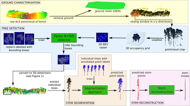
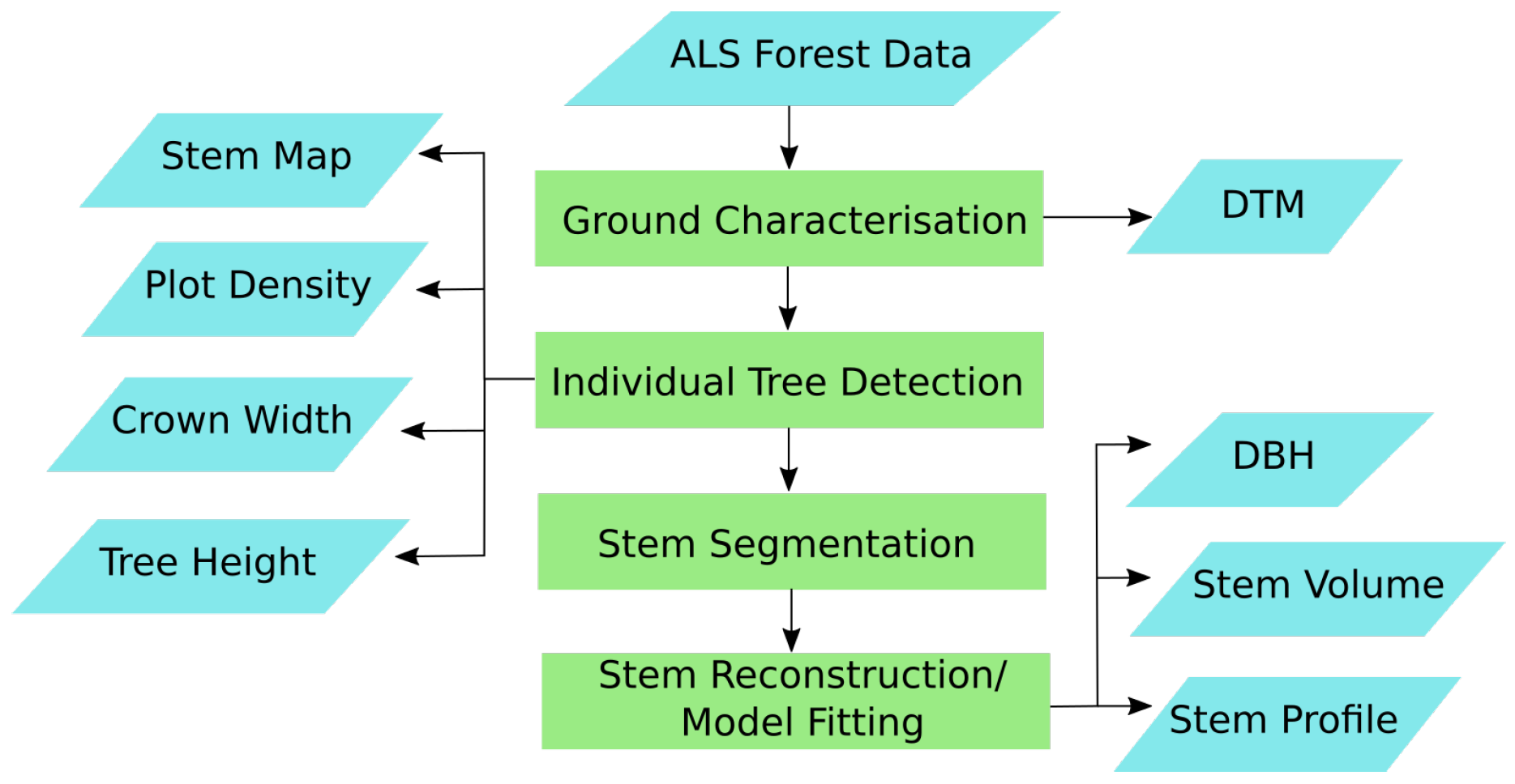
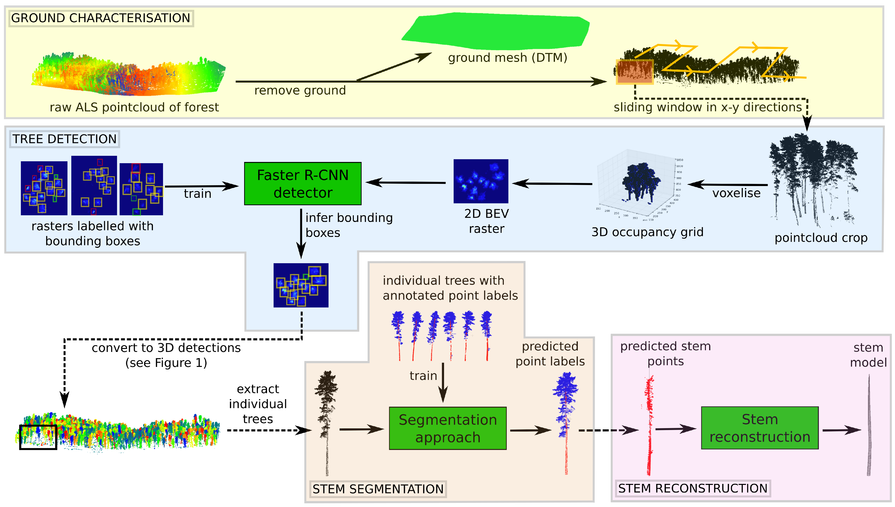
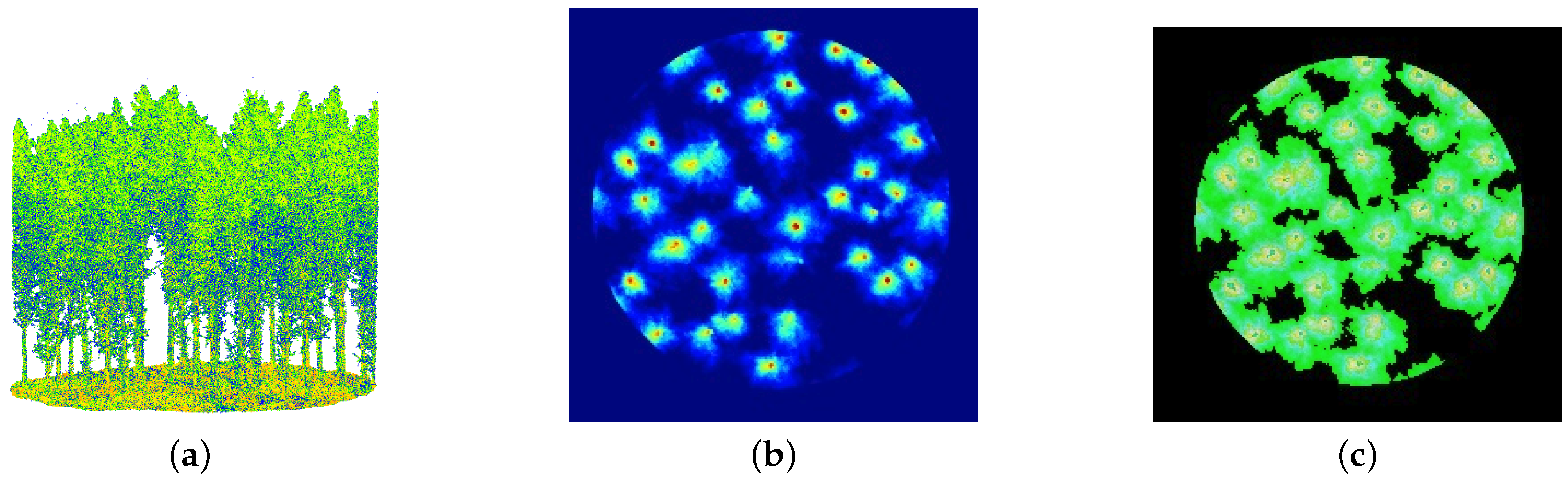
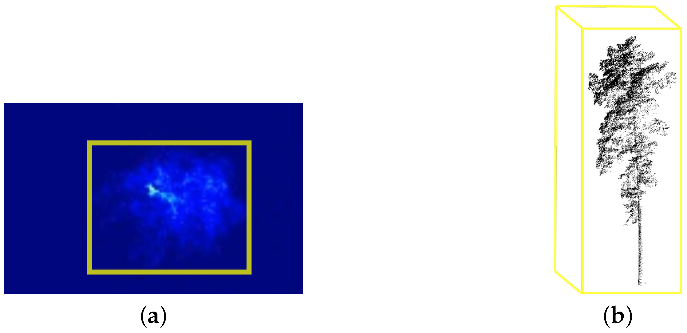
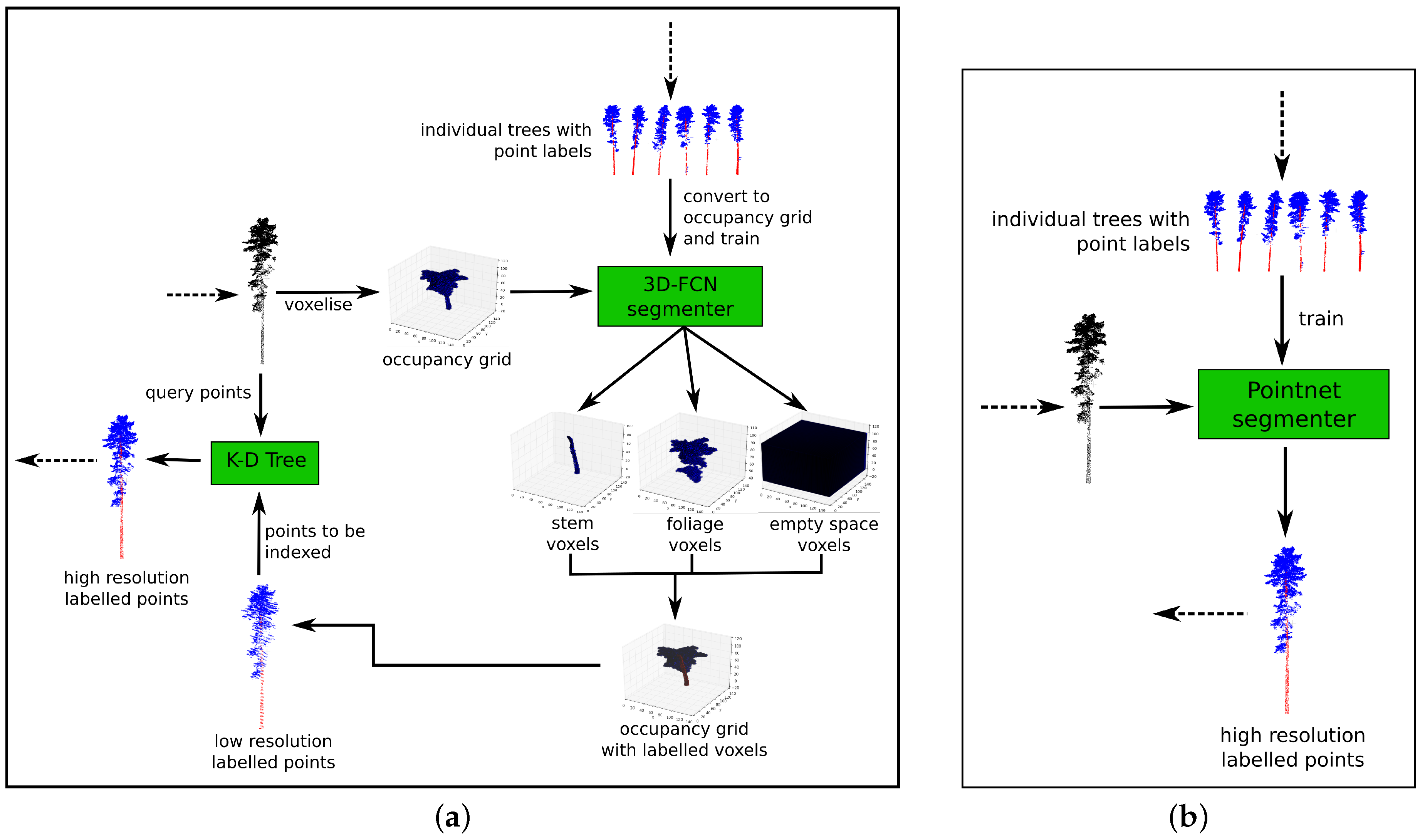
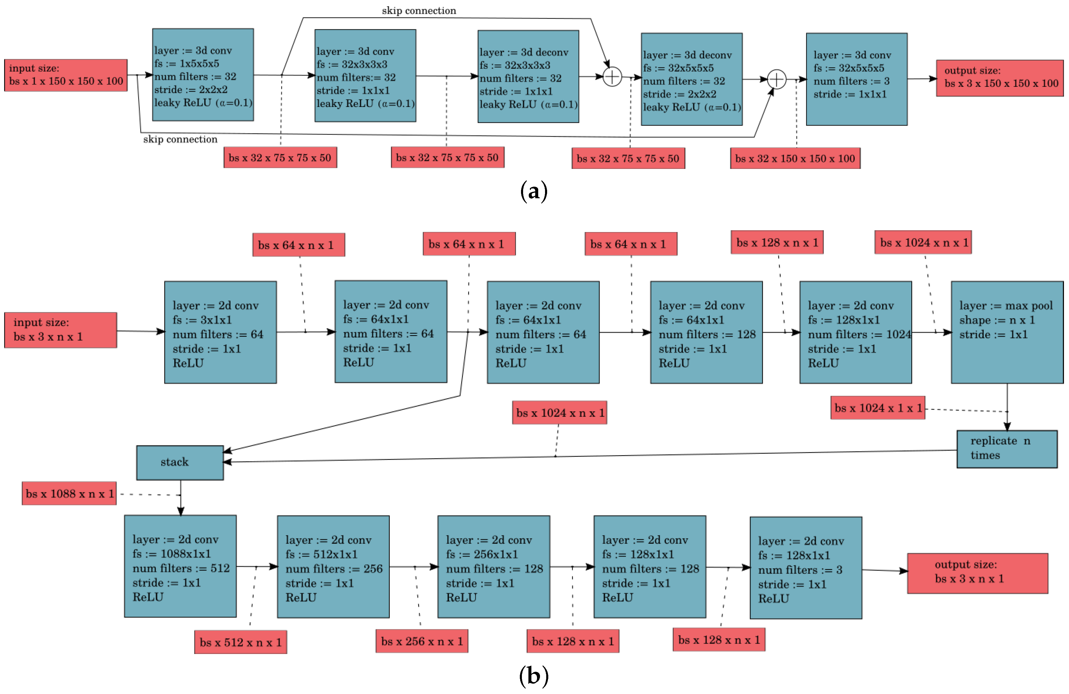
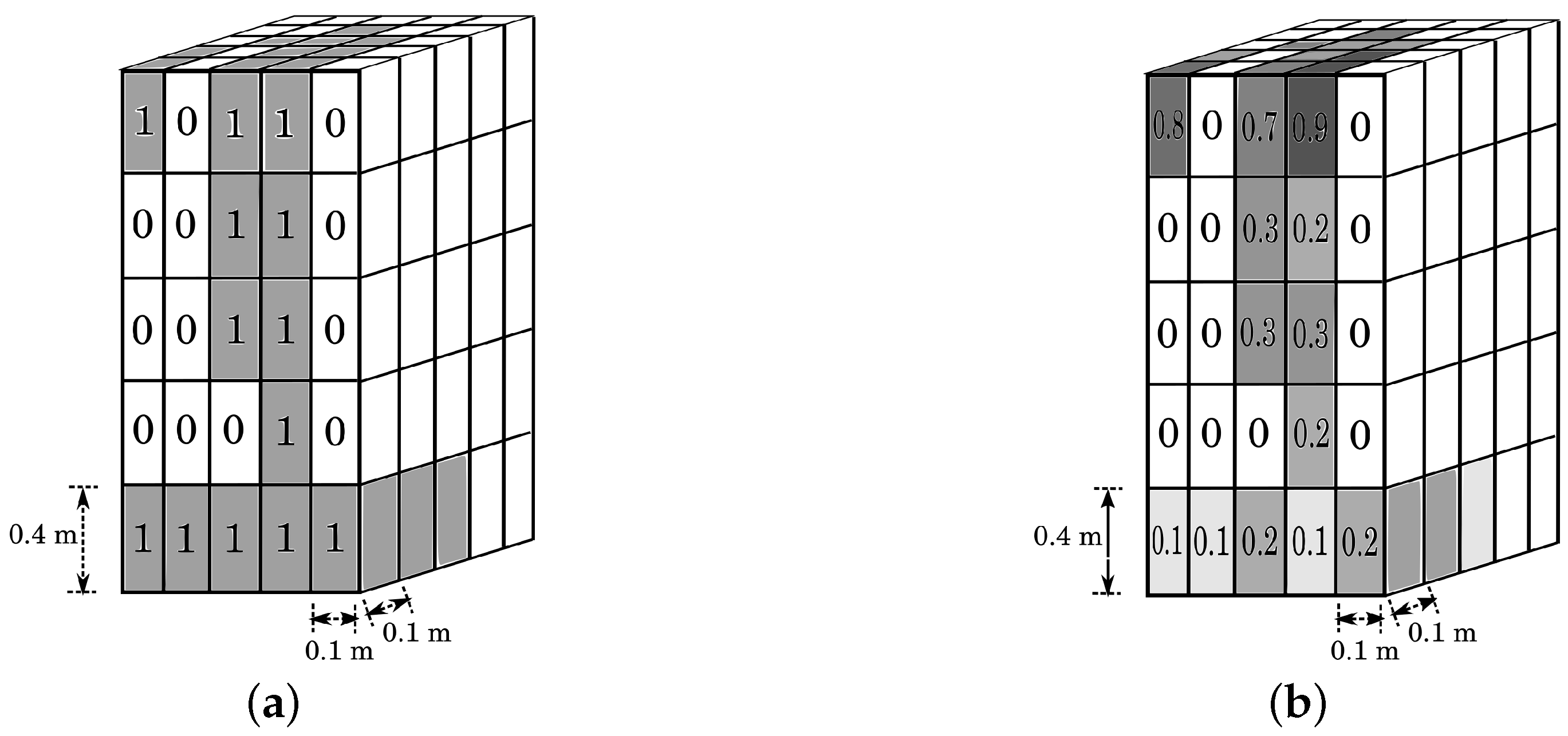
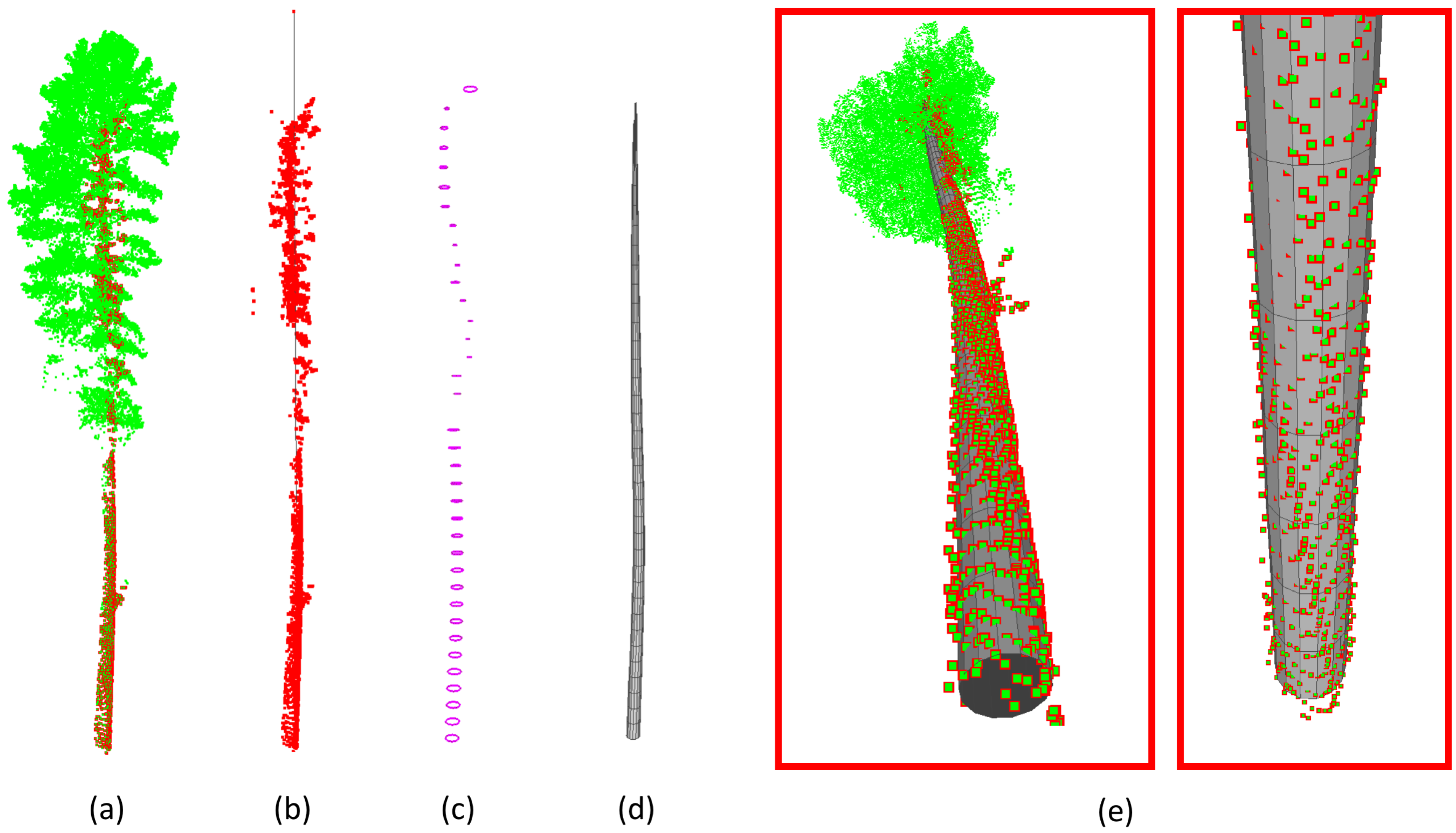
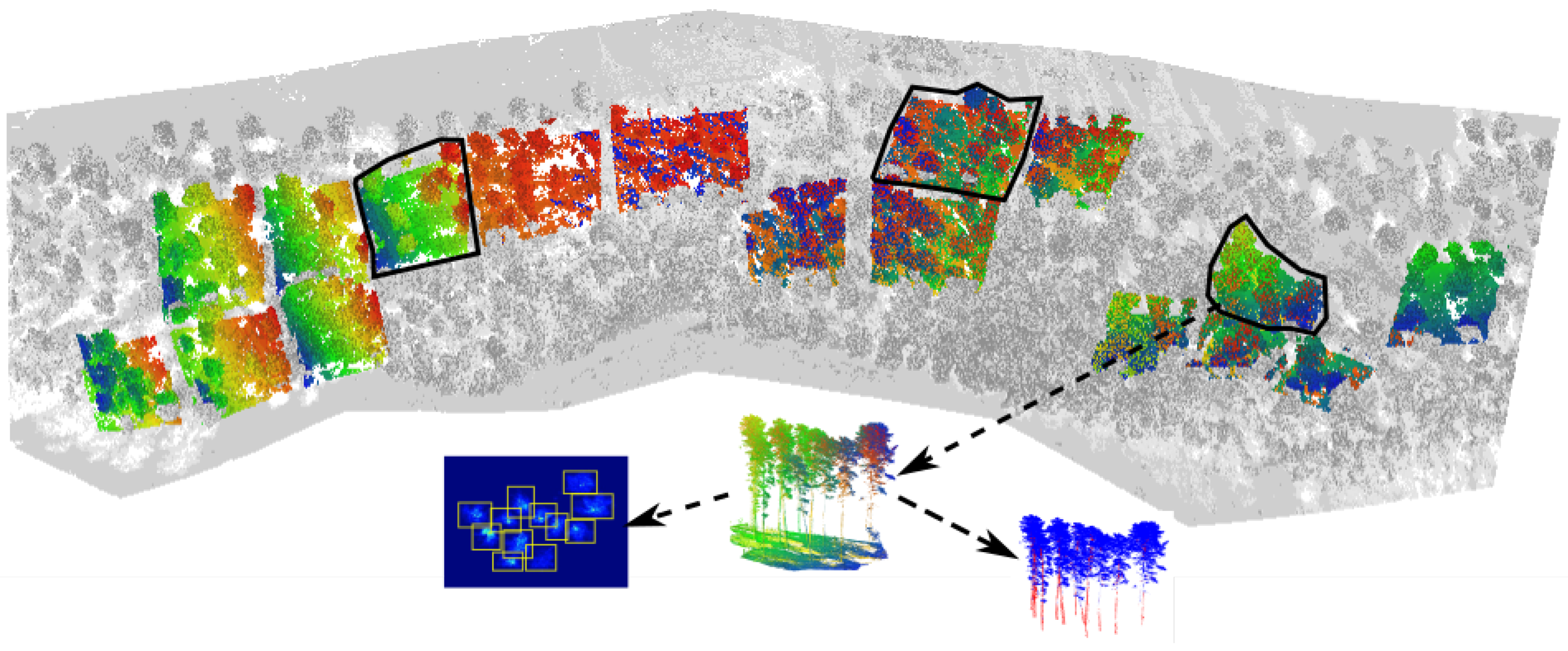
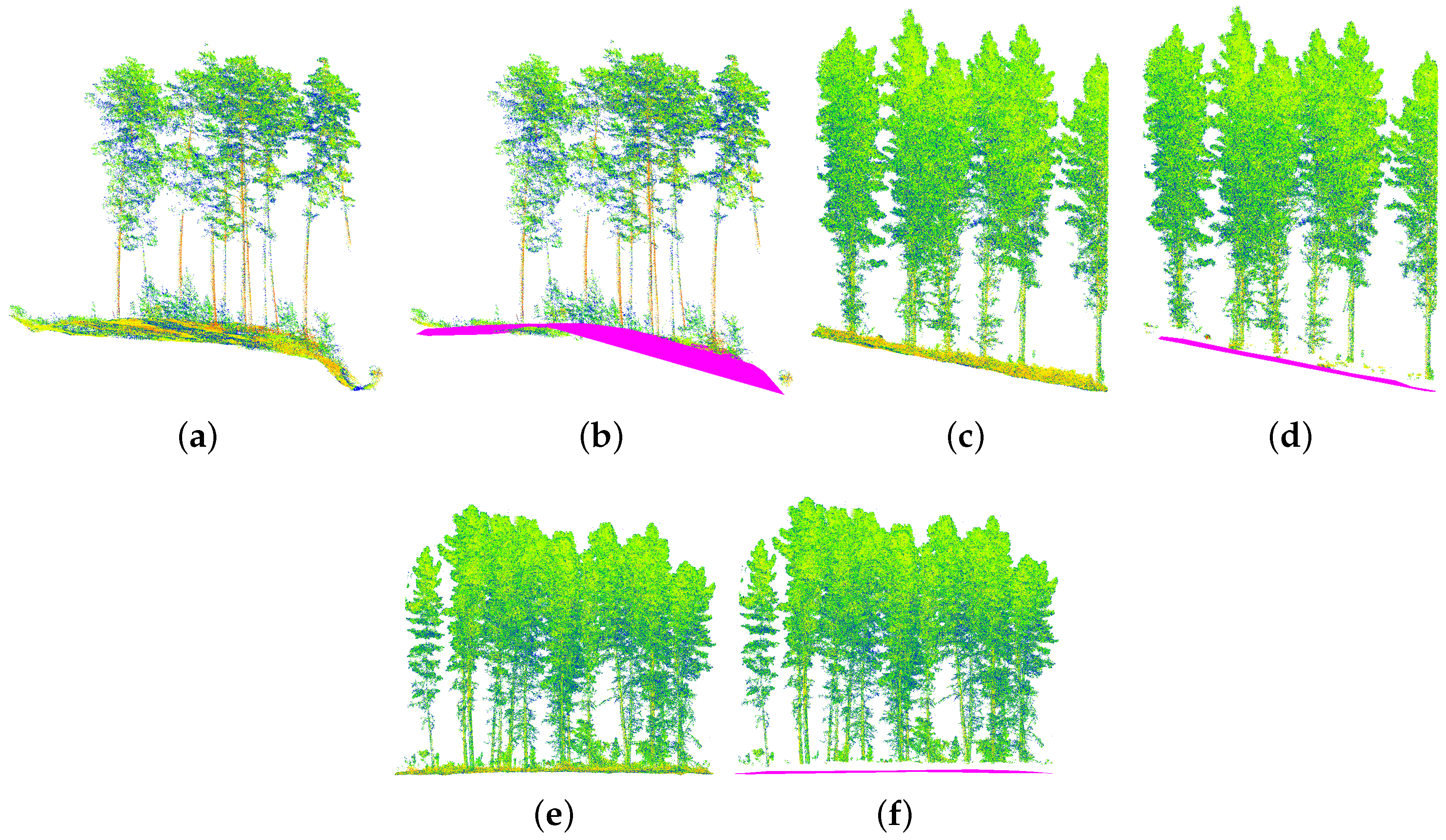
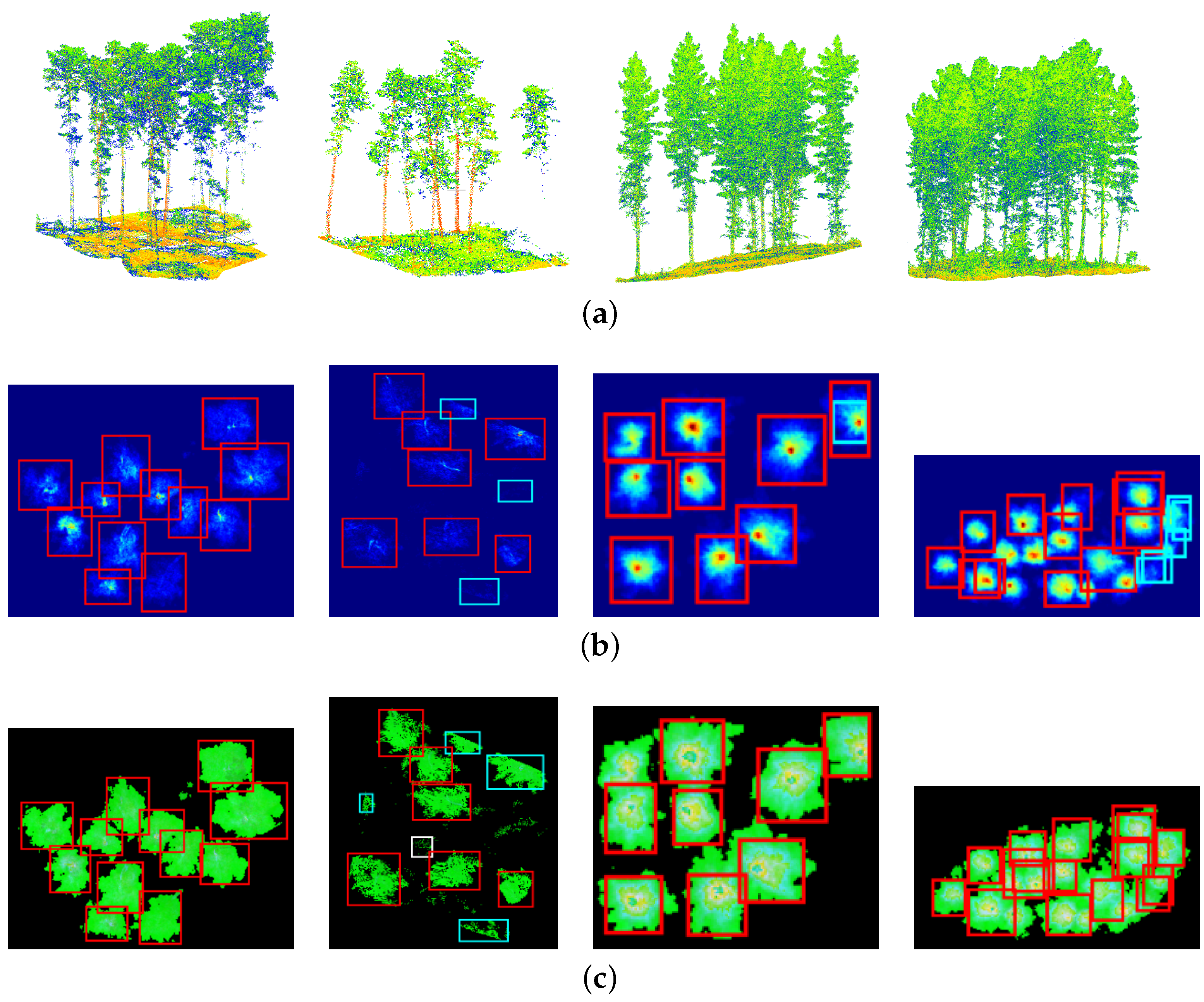
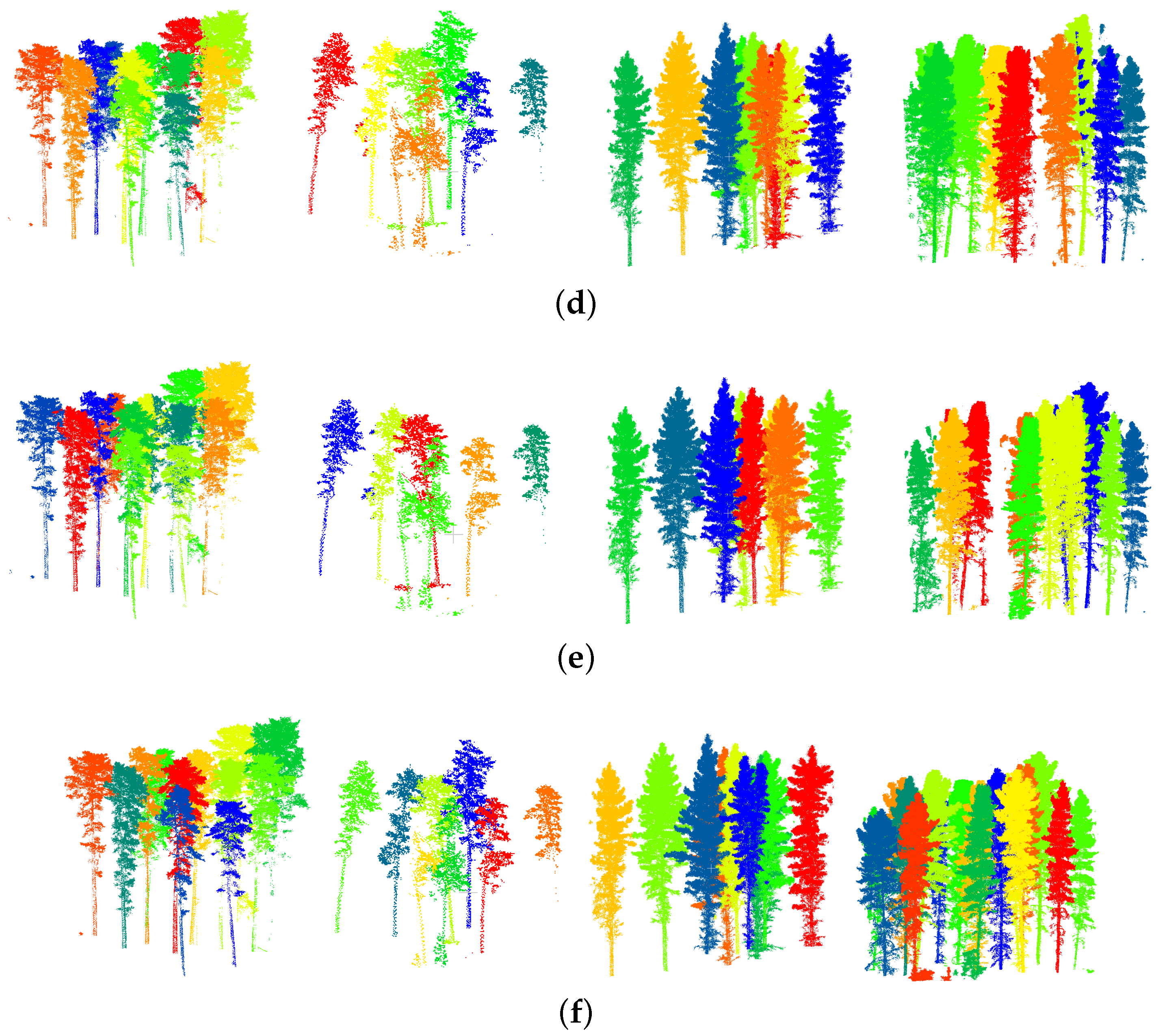
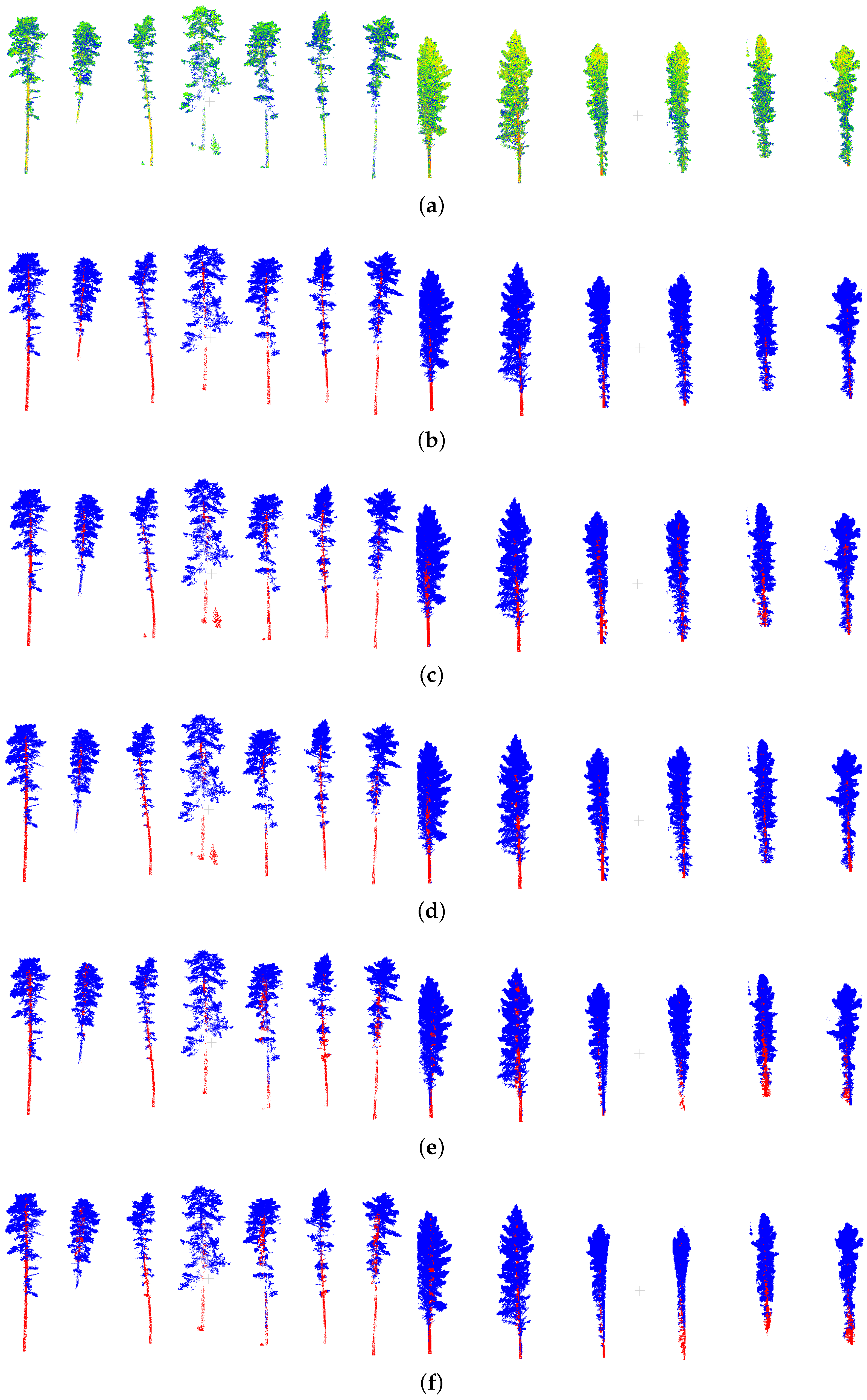
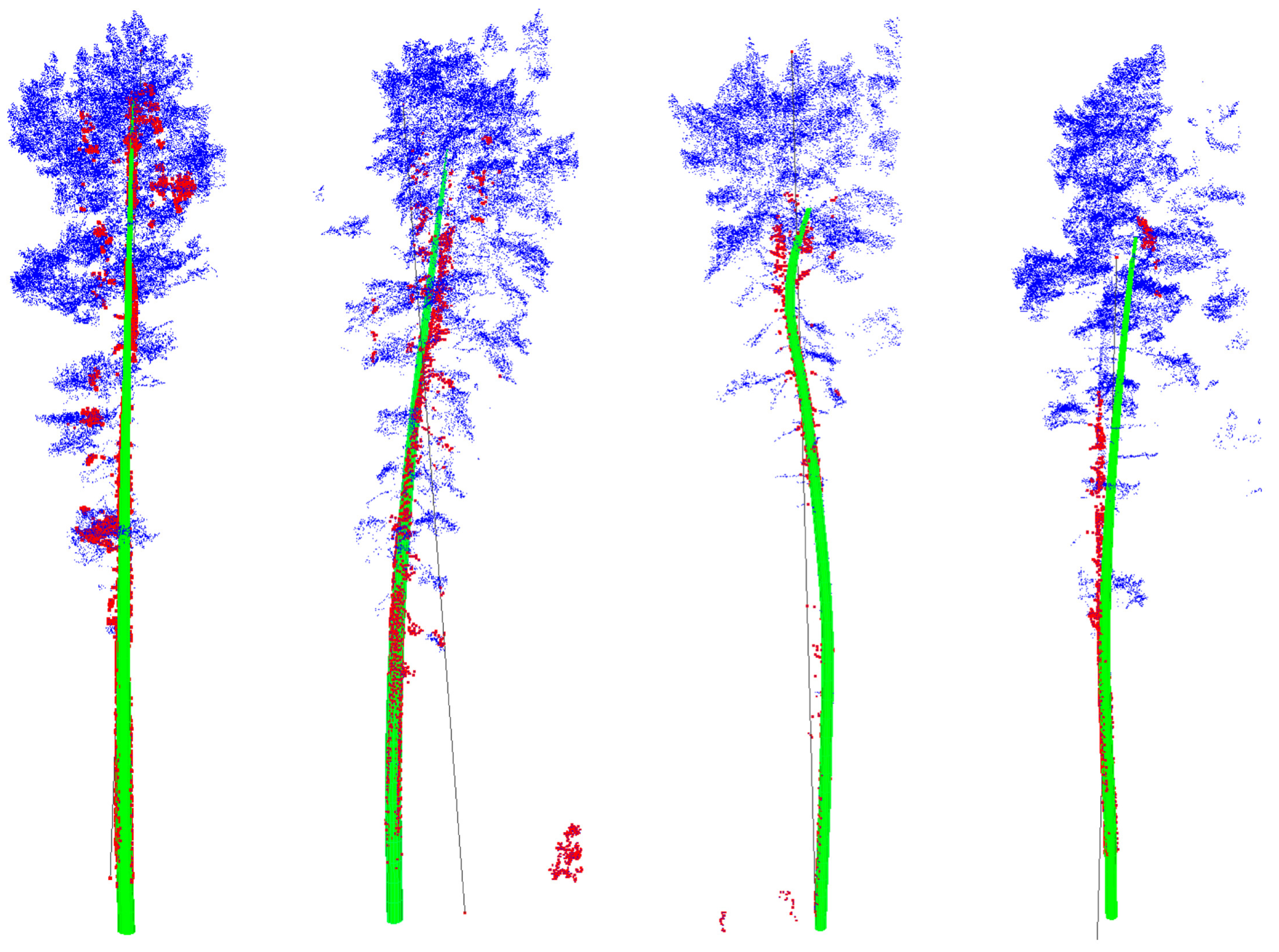
Table 1.
The number of trees used to train, validate and test the segmentation and detection models for each fold of the cross-validation. The test splits did not overlap across folds. Please note that raster bounding box annotations were used to train and validate the detection models, individual tree pointcloud annotations were used to test the detection models and point-level annotations were used to train, validate and test the segmentation models.
| Dataset | Fold | Detection split | Segmentation split | ||||
|---|---|---|---|---|---|---|---|
| Train | Val | Test | Train | Val | Test | ||
| Tumut | 1 | 164 | 12 | 12 | 60 | 3 | 12 |
| 2 | 168 | 12 | 8 | 60 | 7 | 8 | |
| 3 | 165 | 12 | 11 | 60 | 4 | 11 | |
| Carabost | 1 | 233 | 17 | 9 | 66 | 6 | 9 |
| 2 | 216 | 26 | 17 | 60 | 4 | 17 | |
| 3 | 209 | 37 | 13 | 66 | 2 | 13 | |
Table 2.
Individual tree detection cross-validation results comparing methods described in this work (those with a *) with other ALS methods. The acronyms vd, mh and mr stand for vertical density, maximum height and mean return. Detection metrics are described in Section 4.1 (see Equation (9)). The mean and standard deviation across the three folds is reported. The top performing method in each category is highlighted in bold.
| Dataset | Method | Accuracy | Precision | Recall | F1 |
|---|---|---|---|---|---|
| Tumut | CHM + watershed | ||||
| DBSCAN | |||||
| RCNN vd * | |||||
| RCNN vd/mh/mr * | |||||
| Carabost | CHM + watershed | ||||
| DBSCAN | |||||
| RCNN vd * | |||||
| RCNN vd/mh/mr * |
Table 3.
Stem and foliage point segmentation cross-validation results. Methods with a * are those described in this work, and (r) indicates methods which used the LiDAR pulse return information. Please note that the RANSAC approach only extracts stems (does not label foliage). Segmentation metrics are described in Section 4.1 (see Equation (12)). The mean and standard deviation over all trees across the three folds is reported. The top performing method in each category is highlighted in bold.
| Stem | Foliage | ||||||
|---|---|---|---|---|---|---|---|
| Dataset | Method | IoU | Precision | Recall | IoU | Precision | Recall |
| Tumut | Eigen features | ||||||
| Eigen features (r) | |||||||
| RANSAC | |||||||
| Voxel 3D-FCN * | |||||||
| Voxel 3D-FCN (r) * | |||||||
| Pointnet * | |||||||
| Pointnet (r) * | |||||||
| Carabost | Eigen features | ||||||
| Eigen features (r) | |||||||
| RANSAC | |||||||
| Voxel 3D-FCN * | |||||||
| Voxel 3D-FCN (r) * | |||||||
| Pointnet * | |||||||
| Pointnet (r) * | |||||||
Table 4.
DBH errors from reconstructed stems for DBH predicted using stem reconstructions on the manually annotated stem points and DBH predicted using stem reconstructions on the automatically segmented stem points of the full pipeline.
Table 4.
DBH errors from reconstructed stems for DBH predicted using stem reconstructions on the manually annotated stem points and DBH predicted using stem reconstructions on the automatically segmented stem points of the full pipeline.
| DBH Estimates from Manual Seg | DBH Estimates from Pipeline Seg | ||||
|---|---|---|---|---|---|
| DBH RMSE | DBH Max. Error | Avg. Perc. Error | DBH RMSE | DBH Max. Error | Avg. Perc. Error |
| 9.45 cm | 17.2 cm | 9.05% | 15.39 cm | 24.5 cm | 15.85% |
© 2020 by the authors. Licensee MDPI, Basel, Switzerland. This article is an open access article distributed under the terms and conditions of the Creative Commons Attribution (CC BY) license (http://creativecommons.org/licenses/by/4.0/).
Share and Cite
MDPI and ACS Style
Windrim, L.; Bryson, M. Detection, Segmentation, and Model Fitting of Individual Tree Stems from Airborne Laser Scanning of Forests Using Deep Learning. Remote Sens. 2020, 12, 1469. https://0-doi-org.brum.beds.ac.uk/10.3390/rs12091469
AMA Style
Windrim L, Bryson M. Detection, Segmentation, and Model Fitting of Individual Tree Stems from Airborne Laser Scanning of Forests Using Deep Learning. Remote Sensing. 2020; 12(9):1469. https://0-doi-org.brum.beds.ac.uk/10.3390/rs12091469
Chicago/Turabian StyleWindrim, Lloyd, and Mitch Bryson. 2020. "Detection, Segmentation, and Model Fitting of Individual Tree Stems from Airborne Laser Scanning of Forests Using Deep Learning" Remote Sensing 12, no. 9: 1469. https://0-doi-org.brum.beds.ac.uk/10.3390/rs12091469
Note that from the first issue of 2016, this journal uses article numbers instead of page numbers. See further details here.