One-Step Three-Dimensional Phase Unwrapping Approach Based on Small Baseline Subset Interferograms

Abstract

One of the most critical steps in a multitemporal D-InSAR analysis is the resolution of the phase ambiguities in the context of phase unwrapping. The Extended Minimum Cost Flow approach is one of the potential phase unwrapping algorithms used in the Small Baseline Subset analysis. In a first step, each phase gradient is unwrapped in time using a linear motion model and, in a second step, the spatial phase unwrapping is individually performed for each interferogram. Exploiting the temporal and spatial information is a proven method, but the two-step procedure is not optimal. In this paper, a method is presented which solves both the temporal and spatial phase unwrapping in one single step. This requires some modifications regarding the estimation of the motion model and the choice of the weights. Furthermore, the problem of temporal inconsistency of the data, which occurs with spatially filtered interferograms, must be considered. For this purpose, so called slack variables are inserted. To verify the method, both simulated and real data are used. The test region is the Lower-Rhine-Embayment in the southwest of North Rhine-Westphalia, a very rural region with noisy data. The studies show that the new approach leads to more consistent results, so that the deformation time series of the analyzed pixels can be improved.

1. Introduction

1.1. General Aspects and Motivation

Multitemporal differential interferometric (D-InSAR) data are used to detect deformation time series of the Earth’s surface. There are two widely used methods, the Persistent Scatterer Interferometry (PSI) [1] and the Small Baseline Subset (SBAS) method [2]. The two main limitations of interferometry are the spatial and temporal decorrelation which increases with larger baselines between the two SAR images. To eliminate this effect, PSI uses only so called persistent scatterers whose backscattering characteristics, measured by the amplitude of the returning signal, remain stable over time. However, these pixels are very rare, especially in rural areas. Over the years, further methods have been developed to obtain spatially denser results. Two examples are SqueeSAR [3], where both persistent and distributed backscatterers are evaluated together, or the Stanford Method for Persistent Scatterers (STAMPS) [4,5], where the pixel selection is based more on the phase characteristic and less on the amplitude. SBAS, on the other hand, reduces the decorrelation effects by only allowing interferograms between SAR images whose spatial and temporal baselines do not exceed a certain threshold. The SBAS method developed by [2] is based on spatially filtered, so called multilooked interferograms to further reduce the phase noise. Additionally, only pixels with coherence values above a certain threshold are evaluated.

The test region in this work is the Lower-Rhine-Embayment in the southwest of North Rhine-Westphalia, Germany. Within this area, there is one of the largest brown coal areas in Europe with the still active open-cast mines Garzweiler, Hambach, and Inden and the already closed coal mines Sophie-Jacoba in the mining region Erkelenz and Emil Mayrisch in the mining region Aachen. Thus, the Earth’s surface is subject to continuous movements which have to be monitored regularly [6]. D-InSAR data should be used for this purpose. As this is a very rural region, only very few persistent scatterers are available. If the amplitude dispersion index with a typical threshold value of 0.25 is chosen [1], this results in an average of 2.24 persistent scatterers per square kilometer. In order to obtain a denser spatial sampling, the analysis is performed using the SBAS method. In this work, a pixel is defined as stable if its coherence value is greater than or equal to 0.7 in at least 95 percent of the interferograms. This results in an average of 7.65 stable pixels per square kilometer.

The main problem when using interferometric data are that the phase can only be measured modulo 2$\pi$. To derive the information of interest, for instance the deformation, the phase ambiguities have to be solved. This is done in the context of phase unwrapping. In a typical SBAS processing, the phase unwrapping is done iteratively to reduce phase unwrapping errors. However, the phase unwrapping remains a critical task in the analysis [7]. This paper will address this problem and presents a new approach that leads to more consistent results.

1.2. Scientific Context

In many applications, such as magnetic resonance imaging (MRI) or fringe projection profilometry (FPP), the problem of phase ambiguities occurs. In general, the process of phase unwrapping is the reconstruction of an absolute, so called unwrapped phase from the measured wrapped phase. However, this is an ill-posed problem. There is no unique solution unless additional assumptions are made ([8], p. 55). Most methods estimate finite differences between adjacent pixels and assume that these are smaller than half the wavelength. Under this assumption, the phase unwrapping problem is a finite integration problem [9]. In reality, this assumption is rarely true due to noise or a subsampling resulting in a more complex phase unwrapping which depends on the integration path.

A phase image provides information in two dimensions. If measurements are made over time, there is a third dimension: the time. In principle, a distinction is made between spatial and temporal methods. Spatial phase unwrapping methods solve phase ambiguities based on one image. Temporal methods on the other hand solve the phase ambiguities of a phase gradient in time. Therefore, a motion model is derived using the temporal information of this gradient in all images. The estimation of the motion model simplifies the phase unwrapping and is essential for its success. Over the years, many phase unwrapping methods have been developed, whereas especially three-dimensional methods that include both temporal and spatial phase unwrapping became a research focus. The methods developed specifically for FPP data, e.g., [10,11] or the methods developed specifically for MRI data, e.g., [12,13] cannot be applied directly to InSAR data [14]. The radar signal is predetermined by the signal of the satellites, so that, in contrast to FPP or MRI systems, no differently structured patterns or multifrequency methods can be applied.

There are also three-dimensional approaches specifically for D-InSAR data. On the one hand, there are two-step approaches in which the temporal phase unwrapping is carried out first and then in a second step the spatial phase unwrapping follows [7,14]. The disadvantage of this step-by-step approach is that the spatial phase unwrapping destroys the previously established temporal consistency. On the other hand, there are procedures that work in one single step but cannot be easily integrated into the SBAS Workflow [15,16]. These approaches are not based on the temporal and spatial double differences that enter the phase unwrapping algorithm in a typical SBAS workflow.

Currently, there is no three-dimensional approach in the literature that works in one step and is specifically applicable for SBAS interferograms or, to go one step further, that is specifically applicable for spatially filtered so called multilooked SBAS interferograms. This work focuses on the Extended Minimum Cost Flow (EMCF) algorithm [7]. It is a rather popular three-dimensional phase unwrapping method and fully compatible to the SBAS method. The only disadvantage is that it works in two steps. First, each spatial phase gradient is temporally unwrapped. This temporal phase unwrapping is done iteratively for a predefined set of modified observations. These modified observations consist of a linear motion model, whereas the motion model parameters are unknown. The results of the temporal phase unwrapping are then used in the second step to spatially unwrap the phases independently for each image. The temporally unwrapped results serve on the one hand as a starting solution for the spatial phase unwrapping and on the other hand they are used to weight the phase gradients for the spatial phase unwrapping. Three-dimensional phase unwrapping is thus performed by solving two simpler and less dimensional problems. To solve the spatial and temporal phase unwrapping in one step, the EMCF algorithm has to be modified so that the motion model parameters and the weights of the spatial phase unwrapping are estimated independently of the solution of the temporal phase unwrapping. Another point is that the phase unwrapping approach should be applicable for multilooked SBAS interferograms. The multilooking step poses another challenge. Due to this preprocessing step, which is carried out individually for each interferogram, the interferograms are not completely consistent in time. This temporal inconsistency has to be taken into account. Otherwise, the temporal and spatial constraints, combined in one single large constraint matrix, will lead to conflicts.

1.3. Outline

The paper is structured as follows. Section 2 gives an overview of the conventional EMCF approach according to [7]. Afterwards, Section 3 provides some modifications including the estimation of the motion model and the choice of the weights, so that finally in Section 4 a one-step approach can be presented, which is simply integrable into the SBAS Workflow and can also deal with multilooked data. The approach is applied to simulated data and finally, in Section 5, to real data of the Lower-Rhine-Embayment. Section 6 ends with a conclusion.

2. State-of-the-Art Extended Minimum Cost Flow Approach

2.1. Problem Formulation

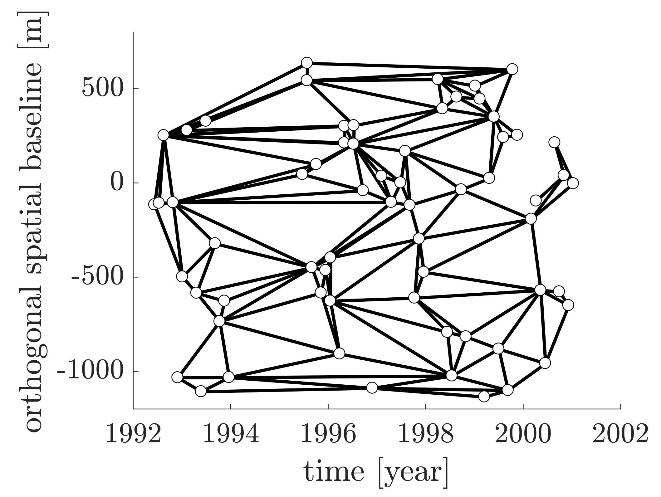
Assume that there is a set ${\mathcal{M}}^{\prime }$ of $m^{\prime }$ SAR images between which a set ${\mathcal{N}}^{\prime }$ of $n^{\prime }$ interferograms is generated according to the SBAS method. This results in a triangulation in the temporal/ perpendicular baseline plane, as shown in Figure 1 for one D-InSAR stack based on ERS 1/2 data from May 1992 to December 2000 as used in the numerical study later on. The white points represent the $m^{\prime }$ SAR images, the black arcs the $n^{\prime }$ interferograms resulting in a set ${\mathcal{R}}^{\prime }$ of $r^{\prime }$ triangles. The triangulation is optimized according to [17]. In order to improve the resulting deformation time series, two preprocessing steps are inserted before the SBAS workflow. These preprocessing steps imply an effective noise filtering and an efficient interferogram selection procedure. It has to be mentioned that this triangulation in the temporal/ perpendicular baseline plane is absolutely necessary for the application of the EMCF algorithm. If the triangulation represents a plane graph, the advantage is that the problem can be solved very efficiently as a network flow problem [18]. However, a triangulation is not absolutely necessary. Ref. [19] allows a free choice of the network in the temporal/ perpendicular baseline plane with overlapping arcs. Thus, the problem can no longer be solved as a network flow problem, but an increased degree of freedom is obtained.

In addition to the triangulation in the temporal/ perpendicular baseline plane, a second triangulation is generated in the azimuth/ range plane. For this purpose, the same set $\mathcal{M}$ of m pixels is evaluated in each interferogram. These pixels have a low noise level, which can be selected, for example, by the coherence value [18]. Based on these pixels, the second triangulation in the azimuth/ range plane is generated. This results in a set $\mathcal{N}$ of n spatial arcs and a set $\mathcal{R}$ of r triangles. The EMCF algorithm proposed by [7] is based on these two triangulations and works in two steps: the temporal and the spatial unwrapping. The algorithm extends the MCF algorithm, originally developed by [18] for the spatial phase unwrapping of one single interferogram. The multitemporal phase unwrapping of the D-InSAR stack is achieved by downscaling the three-dimensional problem into two simpler problems that are two-dimensional. As most phase unwrapping methods, it starts with the estimation of the wrapped phase gradient between two adjacent pixels $x_l$ and $x_k$ within an interferogram with time difference $\Delta t_{\alpha \beta }=t_{\beta }-t_{\alpha }$

$$\begin{array}{c}\hfill {\psi }_{\Delta x_{kl}}^{\Delta t_{\alpha \beta }}={\langle {\psi }_{x_l}^{\Delta t_{\alpha \beta }}-{\psi }_{x_k}^{\Delta t_{\alpha \beta }}\rangle }_{-\pi ,\pi }\forall \Delta x_{kl}\in \mathcal{N}\forall \Delta t_{\alpha \beta }\in {\mathcal{N}}^{\prime }\end{array}$$

(1)

with the modulo 2$\pi$-operator ${\langle .\rangle }_{-\pi ,\pi }$. The wrapped phase gradients differ from the unwrapped ones by an unknown multiple of 2$\pi$

$${\varphi }_{\Delta x_{kl}}^{\Delta t_{\alpha \beta }}={\psi }_{\Delta x_{kl}}^{\Delta t_{\alpha \beta }}+2\pi {\tilde{k}}_{\Delta x_{kl}}^{\Delta t_{\alpha \beta }}$$

(2)

with the unknown phase ambiguity factor ${\tilde{k}}_{\Delta x_{kl}}^{\Delta t_{\alpha \beta }}\in \mathbb{Z}$ of the phase gradient.

2.2. Temporal Phase Unwrapping

First, one spatial phase gradient, for example the gradient $\Delta x_{kl}$, is individually unwrapped in time. With time, the two pixels $x_k$ and $x_l$ are moving with a certain motion model. The relative deformation of this phase gradient is measured in all $n^{\prime }$ interferograms, collected in the wrapped observation vector ${\mathit{\psi }}_{\Delta x_{kl}}^{\Delta t}$. To detect this motion, the temporal information is used to estimate a linear motion model

$$\begin{array}{cc}\hfill M(v_{\Delta x_{kl}},\Delta h_{\Delta x_{kl}})& =\frac{4\pi }{\lambda }\Delta t·v_{\Delta x_{kl}}+\frac{4\pi }{\lambda }\frac{\Delta b_{\perp }}{rsin\left(\theta \right)}·\Delta h_{\Delta x_{kl}}\hfill \end{array}$$

(3)

with the temporal baseline $\Delta t$ and the orthogonal spatial baseline $\Delta b_{\perp }$ between the SAR images, the wavelength $\lambda$, the sensor target distance r in line-of-sight and the incidence angle $\theta$. The error of the scene topography $\Delta h_{\Delta x_{kl}}$ and the deformation velocity variation $v_{\Delta x_{kl}}$ between the pixels $x_k$ and $x_l$ are the unknown parameters. In the following, the model $\mathit{M}(v_{\Delta x_{kl}},\Delta h_{\Delta x_{kl}})$ is briefly referred to as M.

This motion model is used as preliminary information to estimate new modified observations

$${\mathit{\chi }}_{\Delta x_{kl}}^{\Delta \mathit{t}}=\mathit{M}+{\langle {\mathit{\psi }}_{\Delta x_{kl}}^{\Delta \mathit{t}}-\mathit{M}\rangle }_{-\pi ,\pi }$$

(4)

which offer a reduced number of phase ambiguities. This makes the phase unwrapping less complex. The modified and unwrapped gradients differ again by a multiple of 2$\pi$, but this time by a smaller multiple than the original observations ${\mathit{\psi }}_{\Delta x_{kl}}^{\Delta \mathit{t}}$. Thus, the relationship is given by

$$\begin{array}{cc}\hfill {\mathit{\varphi }}_{\Delta x_{kl}}^{\Delta \mathit{t}}& ={\mathit{\chi }}_{\Delta x_{kl}}^{\Delta \mathit{t}}+2\pi {\mathit{k}}_{\Delta x_{kl}}^{\Delta \mathit{t}}\hfill \end{array}$$

(5)

with the unknown phase ambiguity factors ${\mathit{k}}_{\Delta x_{kl}}^{\Delta \mathit{t}}\in {\mathbb{Z}}^{n^{\prime }}$ of the modified phase gradients. Due to some preprocessing steps, e.g., the multilooking which is performed individually to each interferogram, the interferograms are not fully consistent in time. This means that the sum of the unwrapped phase gradients in each of the $r^{\prime }$ triangles of the temporal triangulation, see again Figure 1, is unequal to zero [3,20] resulting in

$$\begin{array}{c}\hfill {\mathit{B}}_{\mathrm{temp}}^T{\mathit{\varphi }}_{\Delta x_{kl}}^{\Delta \mathit{t}}\ne 0\end{array}$$

(6)

with the constraint matrix ${\mathit{B}}_{\mathrm{temp}}^T\in {\mathbb{Z}}^{r^{\prime }\times n^{\prime }}$. One row of ${\mathit{B}}_{\mathrm{temp}}^T$ contains zeros except the columns which belong to the defining arcs of the actual triangle. These are filled with one or minus one depending on the orientation of the arc. If Equation (5) is inserted into Equation (6), the temporal constraint results in

$$\begin{array}{c}\hfill {\mathit{B}}_{\mathrm{temp}}^T{\mathit{k}}_{\Delta x_{kl}}^{\Delta \mathit{t}}=\underset{{\mathit{b}}_{\mathrm{temp}}}{\underbrace{-\lfloor \frac{{\mathit{B}}_{\mathrm{temp}}^T{\mathit{\chi }}_{\Delta x_{kl}}^{\Delta \mathit{t}}}{2\pi }\rceil }}.\end{array}$$

(7)

Due to the temporal inconsistency, the right-hand side ${\mathit{b}}_{\mathrm{temp}}$ will usually not be an integer value and assumes values between $-\pi$ and $\pi$. To ensure that the solution of the unknown phase ambiguity factors ${\mathit{k}}_{\Delta x_{kl}}^{\Delta t}$ will be integer values, the rounding operator $\lfloor .\rceil$ is necessary.

Analogous to the spatial MCF approach proposed by [18], the problem is defined as minimizing the L${}_1$-norm of the phase ambiguity factors

$$\begin{array}{c}\hfill C_{\mathrm{temp}}\left({\mathit{k}}_{\Delta x_{kl}}^{\Delta \mathit{t}}\right)={{\mathit{p}}_{\Delta x_{kl}}^{\Delta \mathit{t}}}^T\left|{\mathit{k}}_{\Delta x_{kl}}^{\Delta \mathit{t}}\right|\dots \min \end{array}$$

(8)

with the weights ${\mathit{p}}_{\Delta x_{kl}}^{\Delta \mathit{t}}$ which are generally set to one for the sake of simplicity. As the constraint matrix ${\mathit{B}}_{\mathrm{temp}}^T$ is totally unimodular and additionally, the weights ${\mathit{p}}_{\Delta x_{kl}}^{\Delta \mathit{t}}$ and the right-hand side vector $b_{\mathrm{temp}}$ have all integer entries, the problem can be solved as a Linear Program (LP) resulting in integer parameters ${\mathit{k}}_{\Delta x_{kl}}^{\Delta \mathit{t}}$ ([21] p. 266). As already mentioned, provided that the triangulation represents a plane graph, the problem can be solved efficiently as a network flow problem [18].

The problem remains that the variables $v_{\Delta x_{kl}}$ and $\Delta h_{\Delta x_{kl}}$ which are included in the sequence of modified observations ${\mathit{\chi }}_{\Delta x_{kl}}^{\Delta \mathit{t}}$ are unknown. Therefore, the parameter vector ${\mathit{k}}_{\Delta x_{kl}}^{\Delta \mathit{t}}$ is sequentially estimated for each ($v_{\Delta x_{kl}}$, $\Delta h_{\Delta x_{kl}}$)-pair in a predefined discrete search space, resulting in one cost function value $C_{\mathrm{temp}}$. The optimal solution is obtained by the pair where the cost value is minimal. This solution is symbolized with a bar afterwards.

2.3. Spatial Phase Unwrapping

In a second step, the temporally unwrapped phase gradients

$${\overline{\mathit{\varphi }}}_{\Delta \mathit{x}}^{\Delta t_{\alpha \beta }}={\overline{\mathit{\chi }}}_{\Delta \mathit{x}}^{\Delta t_{\alpha \beta }}+2\pi {\overline{\mathit{k}}}_{\Delta \mathit{x}}^{\Delta t_{\alpha \beta }}$$

(9)

are used to unwrap each interferogram individually via the spatial MCF approach, c.f. [18]. The previously calculated temporally unwrapped phase gradients ${\overline{\mathit{\varphi }}}_{\Delta x}^{\Delta t_{\alpha \beta }}$ are used as starting point. The problem is again defined as a weighted L${}_1$-norm minimization problem

$$\begin{array}{c}\hfill C_{\mathrm{spatial}}\left({\mathit{k}}_{\Delta \mathit{x}}^{\Delta t_{\alpha \beta }}\right)={{\mathit{p}}_{\Delta \mathit{x}}^{\Delta t_{\alpha \beta }}}^T\left|{\mathit{k}}_{\Delta \mathit{x}}^{\Delta t_{\alpha \beta }}\right|\dots \min \end{array}$$

(10)

under the constraint that the unwrapped phase gradients should be spatially consistent, this time. This means that the sum of the unwrapped phase gradients in each of the triangles in the azimuth/ range plane should be zero, resulting in the constraint

$$\begin{array}{c}\hfill {\mathit{B}}_{\mathrm{spatial}}^T{\mathit{k}}_{\Delta \mathit{x}}^{\Delta t_{\alpha \beta }}=\underset{b_{\mathrm{spatial}}}{\underbrace{-\frac{{\mathit{B}}_{\mathrm{spatial}}^T{\overline{\mathit{\varphi }}}_{\Delta \mathit{x}}^{\Delta t_{\alpha \beta }}}{2\pi }}}\end{array}$$

(11)

with the constraint matrix ${\mathit{B}}_{\mathrm{spatial}}^T\in {\mathbb{Z}}^{r\times n}$ referring to the spatial triangulation in the azimuth/ range plane. As the phase gradients are consistent in space, the right-hand side vector ${\mathit{b}}_{\mathrm{spatial}}$ will be an integer value and a rounding operator is not necessary. The weights ${{\mathit{p}}_{\Delta x}^{\Delta t_{\alpha \beta }}}^T$ in Equation (10) are derived by using the previously calculated temporal cost value ${\overline{C}}_{{\mathrm{temp}}_{\Delta x_{kl}}}$ for the corresponding arc $\Delta x_{kl}$. Large costs mean that the probability of an occurring phase ambiguity is large and therefore the unwrapped phase can be erroneous. Hence, this arc is less familiar and its influence is lowered by low weights. The weights are derived by an inverse exponential relation [7]

$$p_{\Delta x_{kl}}^{\Delta t_{\alpha \beta }}=\left\{\begin{array}{cc}{2}^S/2^{{\overline{C}}_{{\mathrm{temp}}_{\Delta x_{kl}}}}\hfill & {\overline{C}}_{{\mathrm{temp}}_{\Delta x_{kl}}}<\rho \hfill \\ 1\hfill & {\overline{C}}_{{\mathrm{temp}}_{\Delta x_{kl}}}\ge \rho \hfill \end{array}\right.$$

(12)

with an upper limit for the maximum cost $2^S$ and a threshold $\rho$. As the spatial constraint matrix ${\mathit{B}}_{\mathrm{spatial}}^T$ is also totally unimodular, the spatial phase unwrapping can be solved as an LP or due to its special structure as a network flow problem.

3. Modified Extended Minimum Cost Flow Approach

The step-wise EMCF algorithm has the disadvantage that the second spatial phase unwrapping step destroys the previously created temporal constraints in Equation (7). Thus, the aim of this work is the development of a phase unwrapping method that solves the temporal and the spatial phase unwrapping in one single step. Intuitively, the problem seems to be solved simply by putting all the temporal and spatial constraints in one big constraint matrix and by minimizing the weighted L${}_1$-norm of the phase ambiguity factors. However, the problem is that the temporal phase unwrapping is based on the modified observations which include the unknown motion model parameters. These parameters are estimated iteratively by solving the temporal phase unwrapping for a predefined search space and defining these parameters as optimal which cause minimal temporal costs. Furthermore, the results of the temporal phase unwrapping are required to define the weights of the spatial phase unwrapping, see Equation (12). Therefore, the EMCF algorithm has to be modified so that the motion model parameters and the spatial weights are independent of the results of the temporal phase unwrapping.

3.1. Estimation of the Motion Model Parameters

First, the problem of the motion model is discussed. In contrast to the conventional method, where the motion model parameters are defined as optimal, where the temporal cost function is minimal, an alternative approach is used, which has already been discussed and analyzed in [22]. This alternative approach estimates the motion model parameters by searching for the maximum of the Ensemple Phase Coherence (EPC) [23] function. The EPC gives a value for the quality of the estimated model for each phase gradient. For the arc $\Delta x_{kl}$, it is defined as

$$\begin{array}{c}\hfill EPC(v_{\Delta x_{kl}},\Delta h_{\Delta x_{kl}})=\left|\frac{{\displaystyle \sum _{\forall \Delta t_{\alpha \beta }\in {\mathcal{N}}^{\prime }}}{e}^{i({\psi }_{\Delta x_{kl}}^{\Delta t_{\alpha \beta }}-\mathit{M})}}{n^{\prime }}\right|\end{array}$$

(13)

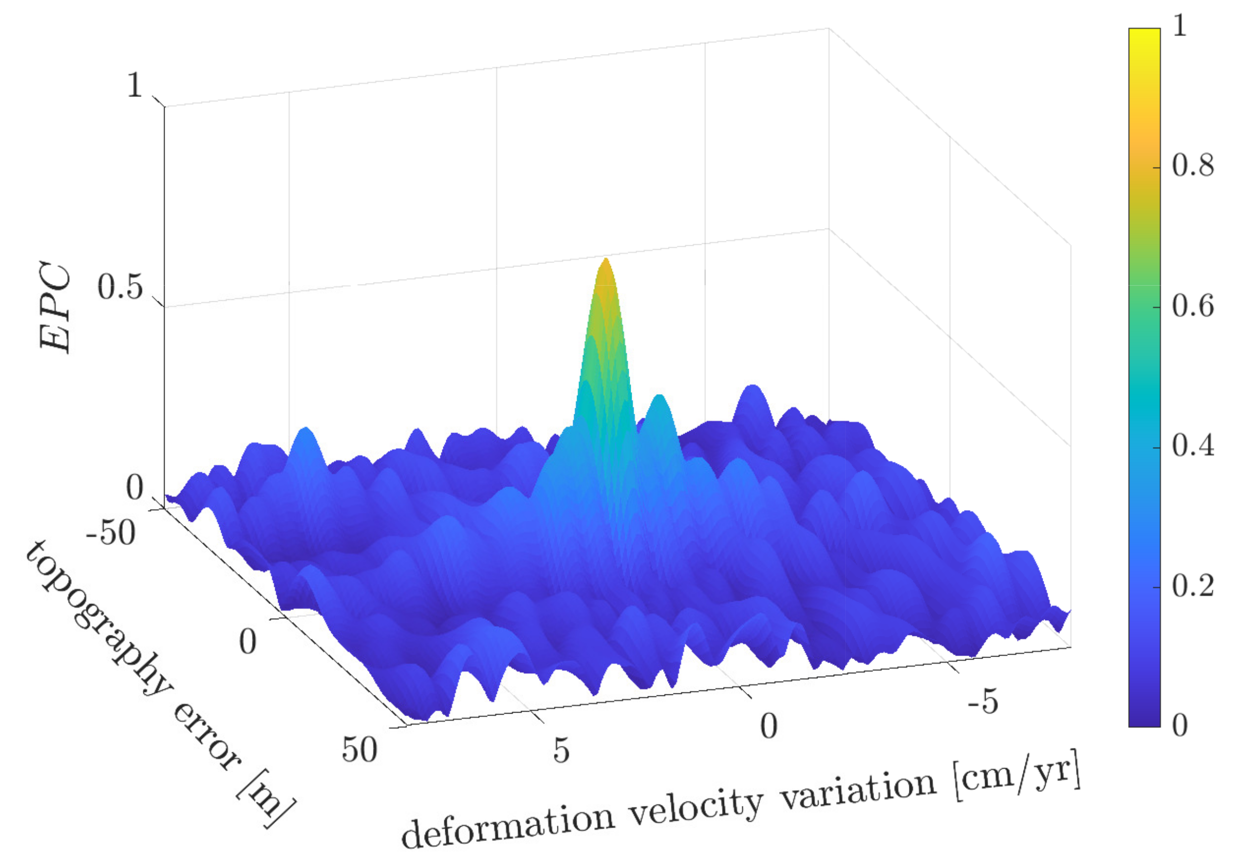
with M from Equation (3) which depends on the parameters $v_{\Delta x_{kl}}$ and $\Delta h_{\Delta x_{kl}}$. The EPC function is continuous with values between zero and one, see the exemplary shown EPC function for one simulated phase gradient in Figure 2. A value of zero means that model and observation do not fit and a value of one corresponds to an optimal fit. It can be seen that the function shows a clear maximum. The idea is to find this maximum of the EPC function and to use the corresponding parameters as optimal motion model parameters to calculate the modified observations, equal to [3]. Especially with noisy data, where the global maximum is not as pronounced, a modified algorithm that combines simulated annealing and the local Nelder–Mead search algorithm is the best way to find the maximum [22]. If the maximum found by simulated annealing falls below a certain threshold, it is assumed that the motion model cannot be estimated reliably enough. Instead of using a possibly too extreme motion model, which is very unreliable and may lead to phase unwrapping errors, the maximum around an appropriate approximate value is locally searched using Nelder–Mead. In contrast to the conventional iterative approach, this alternative approach has the advantage that the motion model can be estimated independently of the temporal phase unwrapping. Consequently, the temporal phase unwrapping only needs to be solved once for each phase gradient. This offers an improved run time. Furthermore, it is no longer necessary to define a discrete search space for the parameters. More information on the analysis and comparison of the alternative and conventional methods can be found in [22].

3.2. Choice of the Weights

The second modification concerns the choice of the weights during the spatial phase unwrapping. Thus far, the spatial weights are derived from an inverse exponential relationship to the temporal costs. Alternatively, the EPC function can be used [19] resulting in

$$\begin{array}{c}\hfill p_{\Delta x_{kl}}\left(EP{C}_{\Delta x_{kl}}\right)=EP{C}_{\Delta x_{kl}}.\end{array}$$

(14)

The higher the EPC value, the better fit observation and model, and the more reliable the result should be. The problem remains that the estimated parameters in form of the phase ambiguity factors $k_{\Delta x}^{\Delta t}$ must be integer values. To get an integer solution from the LP, the weights must also be integers ([21], p. 266). A simple rounding of Equation (14) would only return values of 0 and 1. In order to obtain a slightly more detailed classification, the weight factors are increased by a power of ten and then rounded. An increase by a further power is not necessary. Since only integer values are allowed, the solution is less sensitive to a small change of the weights [24]. In order to obtain a clearer classification, the weight factor is then potentiated to base 2. This results in the following integer weights on the basis of the EPC values

$$\begin{array}{c}\hfill p_{\Delta x_{kl}}\left(EP{C}_{\Delta x_{kl}}\right)=2^{\lfloor EP{C}_{\Delta x_{kl}}·10\rceil }.\end{array}$$

(15)

4. One-Step Three-Dimensional Phase Unwrapping Approach

4.1. Problem Formulation

Using the two modifications described in Section 3, the one-step three-dimensional phase unwrapping approach is defined. Therefore, the two steps, temporal and spatial phase unwrapping, are combined into a single step. However, before the phase unwrapping is performed, it is necessary to estimate the motion model. For this purpose, the EPC function is maximized for each phase gradient using the modified algorithm combining simulated annealing and Nelder–Mead. Based on these modified observations, the multitemporal phase unwrapping is done. For this purpose, the modified observations are all written into a vector

$$\begin{array}{c}\hfill {\mathit{\chi }}_{\Delta \mathit{x}}^{\Delta \mathit{t}}={\left[\begin{array}{cccccccc}{\chi }_{\Delta x_{kl}}^{\Delta t_{\alpha \beta }}& {\chi }_{\Delta x_{kl}}^{\Delta t_{\beta \gamma }}& {\chi }_{\Delta x_{kl}}^{\Delta t_{\gamma \alpha }}& \dots & {\chi }_{\Delta x_{lm}}^{\Delta t_{\alpha \beta }}& {\chi }_{\Delta x_{lm}}^{\Delta t_{\beta \gamma }}& {\chi }_{\Delta x_{lm}}^{\Delta t_{\gamma \alpha }}& \dots \end{array}\right]}^T.\end{array}$$

(16)

Putting all constraints, temporal and spatial ones, into one single constraint matrix $B_{3\mathrm{D}}^T\in {\mathbb{Z}}^{r^{\prime }·n+r·n^{\prime }\times n^{\prime }·n}$, the one-step three-dimensional phase unwrapping approach can be defined as

$$\begin{array}{cc}\hfill \mathrm{Objective}\mathrm{function}:& C_{3\mathrm{D}}\left({\mathit{k}}_{\Delta \mathit{x}}^{\Delta \mathit{t}}\right)={{\mathit{p}}_{\Delta \mathit{x}}^{\Delta \mathit{t}}}^T\left|{\mathit{k}}_{\Delta \mathit{x}}^{\Delta \mathit{t}}\right|\dots \min \hfill \\ \hfill \mathrm{Constraint}:& {\mathit{B}}_{3\mathrm{D}}^T{\mathit{k}}_{\Delta \mathit{x}}^{\Delta \mathit{t}}=\underset{b_{3\mathrm{D}}}{\underbrace{-\lfloor \frac{{\mathit{B}}_{3\mathrm{D}}^T{\mathit{\chi }}_{\Delta \mathit{x}}^{\Delta \mathit{t}}}{2\pi }\rceil }}\hfill \\ \hfill \mathrm{Variable}:& {\mathit{k}}_{\Delta \mathit{x}}^{\Delta \mathit{t}}\in \mathbb{Z}.\hfill \end{array}$$

(17)

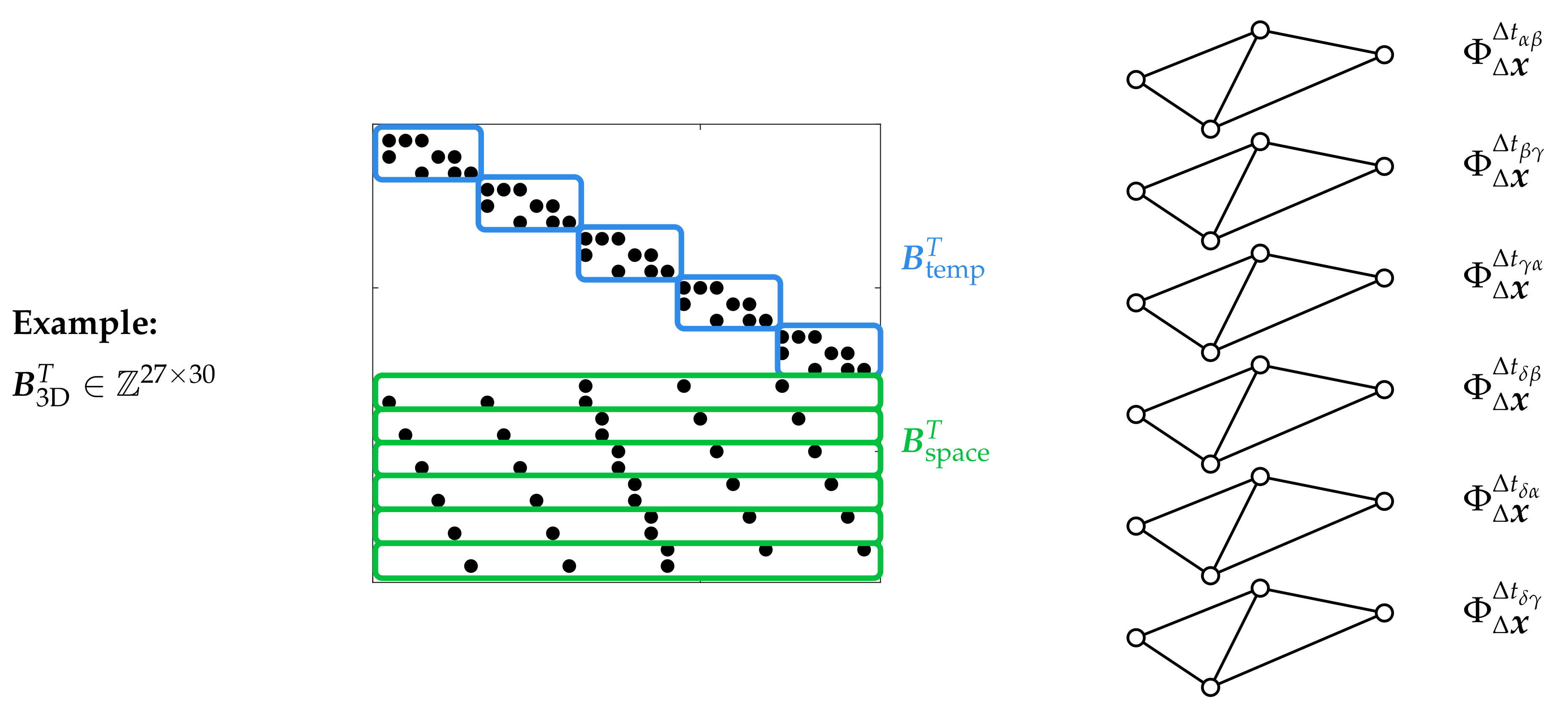
The dimension of the constraint matrix ${\mathit{B}}_{3\mathrm{D}}^T$ quickly becomes large for an entire D-InSAR stack. However, one row of the matrix has only three entries which are non-zero. Therefore, it is a sparse matrix. Figure 3 shows a small D-InSAR stack consisting of $n^{\prime }=6$ interferograms shown in the right subfigure. Each interferogram consists of $n=5$ spatial phase gradients, see black lines between the white points which represent the stable pixels. In time, there exist $r^{\prime }=3$ temporal constraints between the spatial phase gradients. In the left subfigure, the structure of the global constraint matrix is shown. The three temporal constraints fill three rows in the global constraint matrix, see one blue framed block, with three non-zero entries per each row symbolized as black dots. As there are $n=5$ spatial gradients in total, there are five times the blue framed block. The green bordered blocks symbolize the spatial constraints. In each interferogram $r=2$ spatial constraints can be set up. Since there are $n^{\prime }=6$ interferograms in total, six of these green blocks exist. The dimension of the constraint matrix $B_{3\mathrm{D}}^T$ is therefore $3·5+2·6\times 5·6=27\times 30$.

The problem remains of the weights ${\mathit{p}}_{\Delta \mathit{x}}^{\Delta \mathit{t}}$. With this one-step approach, it is no longer possible that the spatial weights are dependent of the temporal costs. Therefore, the EPC based weights, cf. Equation (15), are used to define the weights ${\mathit{p}}_{\Delta \mathit{x}}^{\Delta \mathit{t}}$. Since the EPC value refers to a spatial phase gradient and is the same in all interferograms, the weights are still constant in time and only in space different weights occur for each phase gradient.

4.2. Temporal Inconsistency

A posteriori filtering steps which are done for each interferogram separately, like the multilooking, lead to temporal inconsistent interferograms. For this reason, a rounding operator has to be inserted on the right-hand side of the temporal constraint in Equation (7). A rounding operation always includes errors. It is not clear if rounding down or up represents the truth. Therefore, the rounding can lead to conflicts in the constraints, if the problem is defined in a one-step three-dimensional approach as desired in this work. When formulating the problem in a one-step three-dimensional approach, it must therefore be taken into account that these contradictions are compensated by so called slack variables. The temporal constraints for the phase gradient between the pixels $x_k$ and $x_l$ are thus extended to

$$\begin{array}{c}\hfill {\mathit{B}}_{\mathrm{temp}}^T{\mathit{k}}_{\Delta x_{kl}}^{\Delta \mathit{t}}+{\mathbf{1}}_{[r^{\prime }·n+r·n^{\prime }\times r^{\prime }·n]}y=\underset{{\mathit{b}}_{\mathrm{temp}}}{\underbrace{-\lfloor \frac{{\mathit{B}}_{\mathrm{temp}}^T{\mathit{\chi }}_{\Delta x_{kl}}^{\Delta \mathit{t}}}{2\pi }\rceil }}\end{array}$$

(18)

with the slack variables $y\in {\mathbb{Z}}^{r^{\prime }·n}$. With the help of these slack variables, the temporal inconsistency of the data are compensated. However, it must be avoided that the inclusion of a slack variable replaces the estimation of a phase ambiguity factor. Consequently, the objective function must be adapted accordingly, so that it is expensive to insert such slack variables. Overall, the one-step three-dimensional phase unwrapping can be defined as

$$\begin{array}{cc}\hfill \mathrm{Objective}\mathrm{function}:& C_{3\mathrm{D}}({\mathit{k}}^{\Delta \mathit{t}},y)={{\mathit{p}}_{\Delta \mathit{x}}^{\Delta \mathit{t}}}^T|{\mathit{k}}_{\Delta \mathit{x}}^{\Delta \mathit{t}}|+{{\mathit{p}}_{\mathit{y}}^{\Delta \mathit{t}}}^T\left|\mathit{y}\right|\dots \min \hfill \\ \hfill \mathrm{Constraint}:& \underset{{\mathit{B}}_{3\mathrm{D},y}^T}{\underbrace{\left[\begin{array}{cc}{\mathit{B}}_{3\mathrm{D}}^T& {\mathit{B}}_y^T\end{array}\right]}}\left[\begin{array}{c}{\mathit{k}}_{\Delta \mathit{x}}^{\Delta \mathit{t}}\\ \\ y\end{array}\right]=\underset{{\mathit{b}}_{3\mathrm{D}}}{\underbrace{-\lfloor \frac{{\mathit{B}}_{3\mathrm{D}}^T{\mathit{\chi }}_{\Delta \mathit{x}}^{\Delta \mathit{t}}}{2\pi }\rceil }}\hfill \\ \hfill \mathrm{Variable}:& {\mathit{k}}_{\Delta \mathit{x}}^{\Delta \mathit{t}},y\in \mathbb{Z}\hfill \end{array}$$

(19)

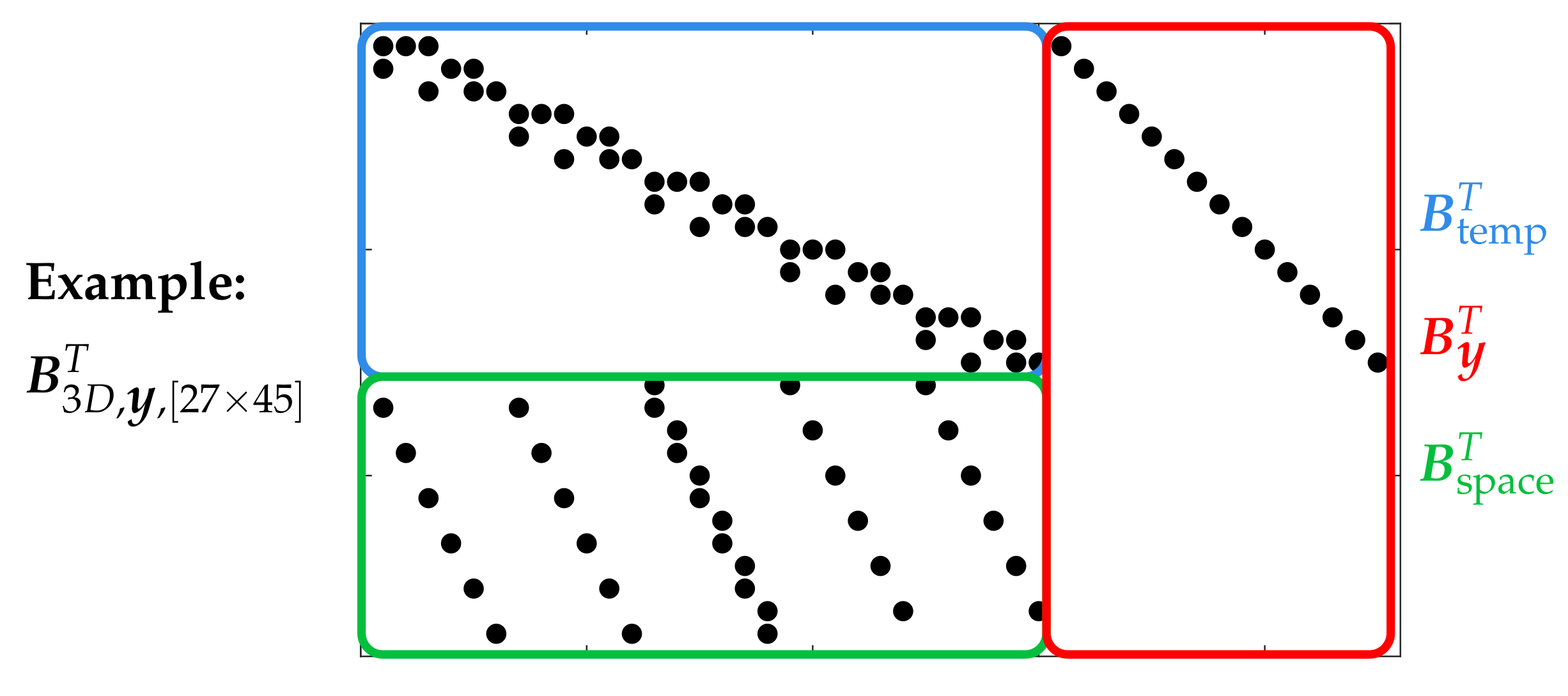
with the constraint matrix ${\mathit{B}}_y^T\in {\mathbb{Z}}^{r^{\prime }·n+r·n^{\prime }\times r^{\prime }·n}$, which consists of an identity matrix for the temporal constraints and has only zero columns for the spatial constraints. Thus, the whole constraint matrix ${\mathit{B}}_{3\mathrm{D},y}^T$ expands to a dimension of $r^{\prime }·n+r·n^{\prime }\times n^{\prime }·n+r^{\prime }·n$. For the above example, the global matrix is extended by the columns framed in red, see Figure 4. A slack variable is added for each of the $3·5$ temporal constraints. Thus, the constraint matrix ${\mathit{B}}_{3\mathrm{D},y}^T$ gets a size of $27\times 30+3·5=45$. However, there are a maximum number of four non-zero entries per row, so that the matrix is sparse again. The weights of the slack variables ${\mathit{p}}_{\mathit{y}}^T$ must be chosen very high, so that it is more expensive to insert a slack variable than to estimate a phase ambiguity factor. The constraint matrix remains totally unimodular, so that the phase unwrapping can still be solved with standard LP solvers resulting in integer parameters. The observations represent double differences in space and time based on two graphs, one in the temporal/ perpendicular baseline plane and the other one in the azimuth/ range plane. However, it is not possible to represent the observations in a three-dimensional graph, so the one-step approach can no longer be defined as a network flow problem. Similar to [19], this enables the potential to select other D-InSAR distributions with overlapping arcs in the temporal/ perpendicular baseline plane.

4.3. Application to Simulated Data

4.3.1. Simulation Scenario

The one-step three-dimensional approach described in Equation (19) shall be applied to a simulated D-InSAR stack and compared with the conventional EMCF algorithm [7]. The ERS 1/2 data from May 1992 to December 2000, which cover the test region of the Lower-Rhine-Embayment, serve as data basis. Based on the temporal and spatial configuration of the 64 SAR images, a settlement depression is simulated related to the first image. The test region is limited to 401 × 401 pixels with the settlement depression in the center. The deformation consists of a linear trend where the mean deformation velocity is limited to a range from 8 to 12 cm/yr. The deformations within the subsidence basin of the still active open-cast mine Garzweiler, Hambach, and Inden are in a comparable range of values, so that the simulation is realistic. In addition to the deformation, a topography error is added. This reaches values between −5 and 40 m. To make the simulation more realistic, a normally distributed noise is added per SAR image. The standard deviation varies from 0.2 to 0.9 rad. The typical signal-to-noise ratio for ERS data are 10 to 20 db ([25], p. 26) corresponding to 0.3 to 0.7 rad [26]. Between the 64 SAR images, 161 interferograms are generated according to the SBAS method resulting in 98 temporal constraints, see the corresponding temporal triangulation already shown in Figure 1. Since the interferograms are spatially filtered, the real data are not consistent in time. To simulate this, an additional normally distributed noise is added to each simulated interferogram. The standard deviation depends on the unbiased coherence [27] taken from the real data. These coherence values are also used to select the so called stable pixels. A pixel is defined as stable if it has a coherence value greater than or equal to 0.7 in at least 95% of the interferograms. Within the 401 × 401 test region, this is the case for $m=9346$ pixels defining $n=27,900$ arcs and $r=18,555$ spatial constraints.

4.3.2. Results of Closed Loop Simulation

The simulated phase serves as the reference phase. This phase is wrapped in a value range from $-\pi$ to $\pi$ representing the measured phase which has to be unwrapped multitemporally. In the best-case scenario, the unwrapped phase will then return to the reference phase. To multitemporally unwrap the measured phases, the conventional EMCF algorithm [7] is used first. In addition, an alternative EMCF algorithm is applied, where the motion model parameters are estimated by maximizing the EPC function using the modified algorithm and where EPC based weights are used. Finally, the phase ambiguities are solved using the one-step three-dimensional phase unwrapping approach.

The first validation criterion is the temporal consistency. Due to the insertion of slack variables, the results of the one-step approach will not be completely consistent in time. As explained above, this is mostly not the case due to preprocessing steps such as multilooking. However, it is assumed that the results of the one-step approach are more consistent than the results of the two-step EMCF approach. To validate the temporal consistency, the absolute number of temporal inconsistencies is calculated for each phase gradient

$$\begin{array}{c}\hfill TIN{C}_{\Delta x_{kl}}=\sum \left|\lfloor \frac{{\mathit{B}}_{\mathrm{time}}^T{\mathit{\varphi }}_{\Delta x_{kl}}^{\Delta \mathit{t}}}{2\pi }\rceil \right|\forall \Delta x_{kl}\in \mathcal{N}\end{array}$$

(20)

and again summarized for all phase gradients, resulting in

$$\begin{array}{c}\hfill TINC=\sum _{\forall \Delta x_{kl}\in \mathcal{N}}TIN{C}_{\Delta x_{kl}}.\end{array}$$

(21)

Table 1. Total number of temporal inconsistencies for different noise levels. In addition to the reference, the number is listed for different phase unwrapping methods.

Method	Total Number of Temporal Inconsistencies for Different Noise Levels [rad]
	0.2	0.4	0.6	0.8	0.9
reference	59	59	59	59	59
conventional EMCF approach	23	23	46	30,705	142,090
alternative EMCF approach	33	19	88	28,336	65,599
one-step three-dimensional approach	14	14	14	14	14

lists the total number of temporal inconsistencies for different noise levels and different phase unwrapping methods. For comparison, the number of the reference phases is also shown. Since the noise is added per SAR image, the number of temporal inconsistencies remains the same for different noise levels. This is the case with the solution of the one-step approach. It is also obvious that the one-step approach provides the most consistent results. The solution is even more consistent than the reference data. If the noise level is lower, the other two methods also provide a lower number of temporal inconsistencies than the reference. However, especially at higher noise levels, it becomes obvious that the conventional EMCF algorithm leads to significantly more inconsistencies. The alternative EMCF approach can reduce the temporal inconsistencies somewhat, but also here the spatial phase unwrapping that follows in the second step destroys the temporal consistencies previously created in the temporal phase unwrapping.

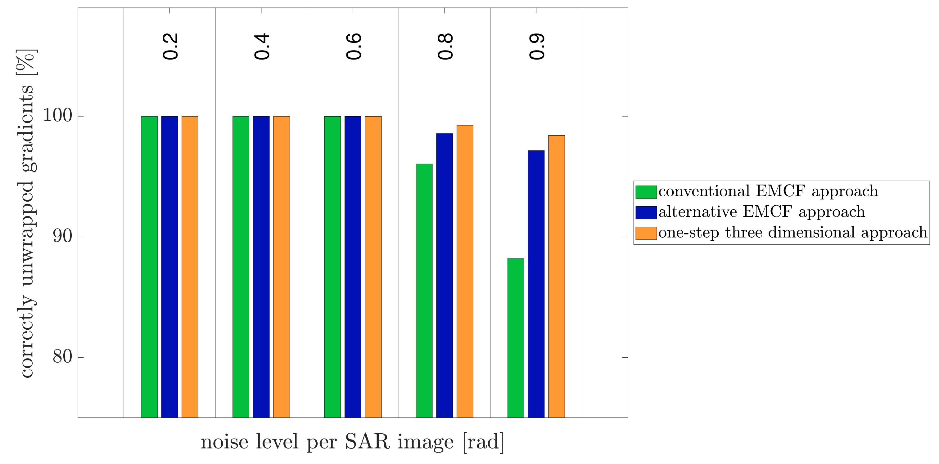
Since the reference number is never reproduced exactly, the accuracy of the results is further investigated. Therefore, Figure 5 shows the percentage of correctly unwrapped phase gradients depending on the noise level. The green bars represent the results of the conventional EMCF algorithm, the dark blue bars of the alternative EMCF algorithm, and the orange bars of the new one-step method. Up to a noise level of 0.6 rad, there are no significant differences. Nearly all phase gradients are unwrapped correctly. Above a noise level of 0.8 rad, it looks different. The alternative EMCF algorithm shows an improvement compared to the conventional approach. At a noise level of 0.8 rad, the number of correctly unwrapped phase gradients increases from 96.05% to 98.56% and at a noise level of 0.9 rad from 88.24% to 97.15%. By applying the one-step three-dimensional method, the percentage can be increased even further to 99.26% at a noise level of 0.8 rad and to 98.41% at a noise level of 0.9 rad.

5. Application to Real Data

5.1. Data Basis

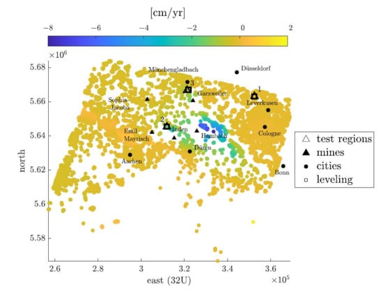
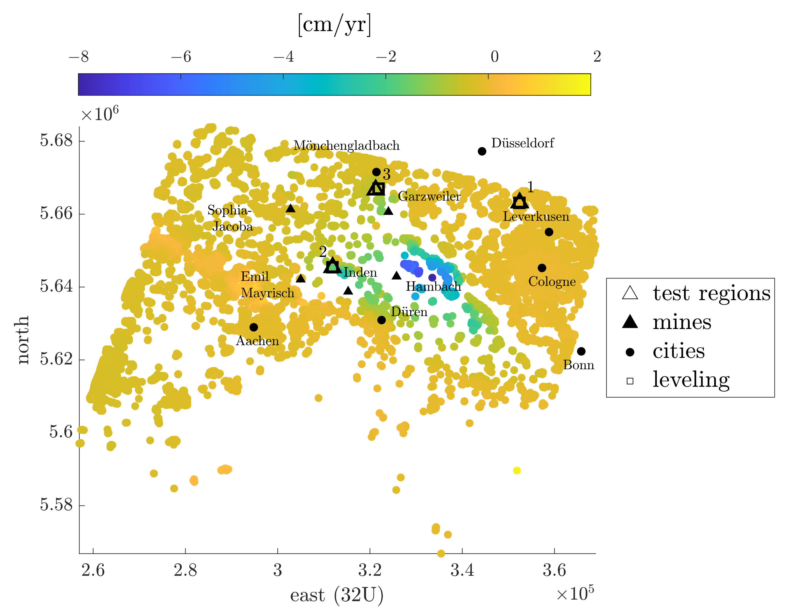
In the following, it will be tested if the one-step three-dimensional approach also leads to better results when applied to ERS 1/2 real data. The test region is the Lower-Rhine Embayment in North Rhine-Westphalia, Germany with the still active open-cast mines Garzweiler, Hambach and Inden and the already closed coal mines Sophie-Jacoba in the mining region Erkelenz and Emil Mayrisch in the mining region Aachen. Analogous to the simulation, the data consist of $m^{\prime }=64$ SAR images collected from May 1992 to December 2000. The temporal triangulation is already shown in Figure 1. A total of $n^{\prime }=161$ D-InSAR images are generated according to the SBAS method resulting in $r^{\prime }=98$ temporal constraints. The SBAS analysis is carried out with the Remote Sensing Software Graz (RSG) (http://www.remotesensing.at/en/remote-sensing-software.html). Pixels are defined as coherent when their coherence values are greater than or equal to 0.7 in at least 95% of the interferograms. For the whole ERS 1/2 scene, this is the case for $m=96,531$ pixels defining $n=289,489$ arcs and $r=192,959$ triangles. Figure 6 shows the mean deformation velocity map of the coherent pixels using the conventional EMCF approach which is the state of the art in the RSG software. Since the phase gradients represent temporal and spatial double differences, there is a datum defect. To overcome this defect, both a temporal and a spatial reference must be chosen. The spatial reference is a pixel in Cologne, since it can be assumed that this region is stable. In time, the first SAR image in May 1992 serves as reference. In Figure 6, it is clearly visible that the Earth’s surface decreases by −6 to −8 cm/yr around the still active open-cast mines Garzweiler and Hambach and increases by a few cm/yr near the closed coal mines Sophie-Jacoba in the mining region Erkelenz and Emil Mayrisch in the mining region Aachen.

The SBAS analysis is repeated, whereas this time the phase unwrapping is performed externally in MATLAB© (R2019b, The MathWorks, Natick, MA, USA) once using the alternative EMCF algorithm and once using the new one-step approach. The deformation maps are very similar to that shown in Figure 6. The average difference is only 0.004 cm/yr in both cases. Therefore, other criteria have to be found to compare the results.

5.2. Temporal Consistency

Similar to the simulated data, the total sum of temporal inconsistency is calculated according to Equation (21). As a reminder, the phase unwrapping is carried out iteratively during the SBAS analysis to reduce phase unwrapping errors. Therefore, the total number of temporal inconsistency is calculated once after the first and once after the second phase unwrapping, see

Table 2. Number of total temporal inconsistencies for ERS 1/2 data. The number is listed for different phase unwrapping methods after the first and the second phase unwrapping step in the SBAS workflow.

Method	Total Number of Temporal Inconsistencies after
	1st Phase Unwrapping	2nd Phase Unwrapping
conventional EMCF approach	16,309	2947
alternative EMCF approach	15,711	2810
one-step three-dimensional approach	10,491	938

. The values clearly show that the conventional EMCF approach leads to most temporal inconsistencies. The alternative EMCF approach shows a slight improvement and the one-step three-dimensional approach shows the most consistent results.

5.3. Smoothness in Space

The second criterion is the smoothness in space. It is assumed that no large movements should occur between adjacent pixels. Therefore, the Root Mean Square (RMS) error is calculated for each pixel $x_j$ in space. For each pixel $x_j\in \mathcal{M}$, there is a deformation time series $h_{x_j}^{t_{\alpha }},\forall t_{\alpha }\in {\mathcal{M}}^{\prime }$. This deformation time series is compared to the deformation time series of the set ${\mathcal{M}}_{x_j}$ of $m_{x_j}$ pixels within a radius of 300 m around $x_j$. If at least five pixels lie within this radius, the difference between the deformation time series of the analyzed pixel and the individual pixels within the radius is squared and averaged over the number of $m_{x_j}$ pixels. Then, the average over all $m^{\prime }$ time acquisitions is taken to obtain one RMS value for each pixel

$$\begin{array}{c}\hfill RM{S}_{x_j}=\frac{1}{m^{\prime }}\sum _{t_{\alpha }\in {\mathcal{M}}^{\prime }}\sqrt{\sum _{x_k\in {\mathcal{M}}_{x_j}}{(h_{x_k}^{t_{\alpha }}-h_{x_j}^{t_{\alpha }})}^2/m_{x_j}},\forall x_j\in \mathcal{M}.\end{array}$$

(22)

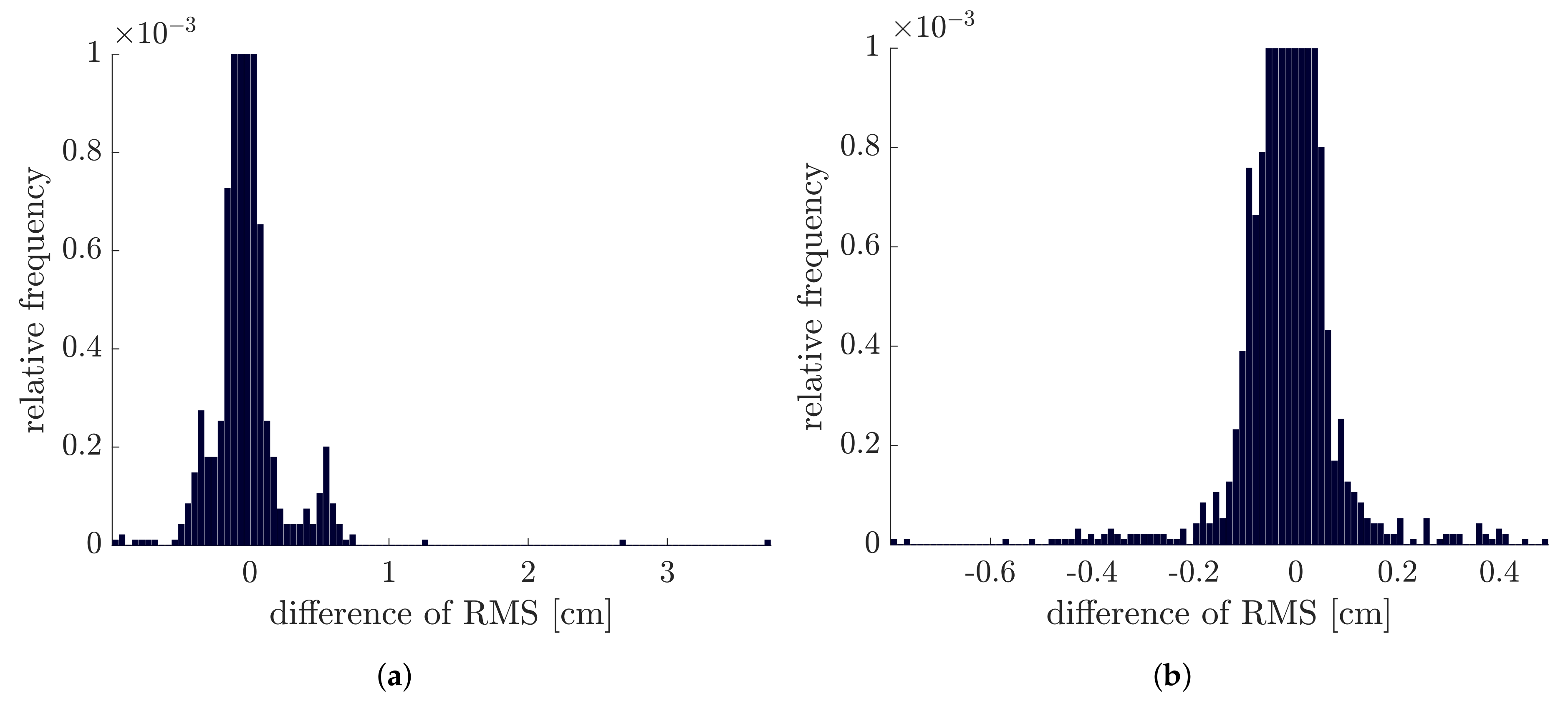
In this way, the RMS is calculated for 89.4% of pixels for the results of the conventional and the alternative EMCF approach and for the results of the one-step three-dimensional approach. Figure 7a shows the comparison between the conventional method and the one-step approach. The difference of the RMS value of the methods is formed in such a way that positive differences indicate that the RMS value is lower when using the one-step approach. The differences are mostly all close to zero. The histogram shows the relative frequencies, which sum up to one. The bar around zero thus goes almost to one. In order to make anything visible, the histogram has been cut off. There are also RMS differences of a few centimeters, for example 2.8 cm, which corresponds to half a wavelength and thus indicates phase unwrapping errors. These larger differences are in the positive range, so that the one-step three-dimensional approach leads to a reduction of the RMS value. Figure 7b shows analogously the histogram of the differences between the alternative EMCF and the one-step three-dimensional approach. Here, again, the histogram is truncated at the top. Positive differences also mean that the one-step approach leads to lower RMS values than the alternative EMCF approach. However, it can be seen that the differences are very small and less than 1 cm. Consequently, by just comparing the RMS values, it is not possible to say which approach delivers better and which worse results.

5.4. Single Pixel Evaluation

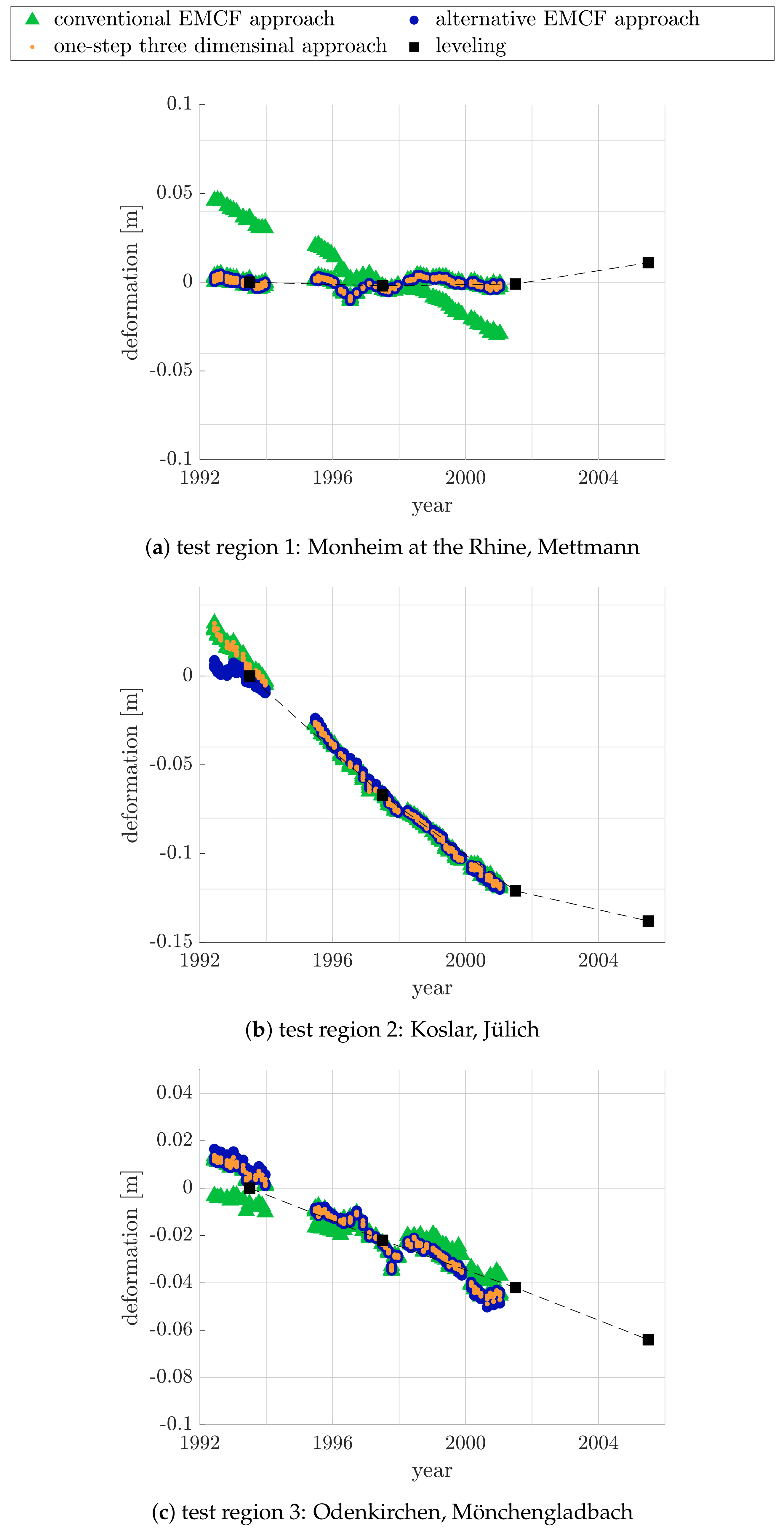
For a further investigation, the time series of five pixels located in the three test regions highlighted in Figure 6 are analyzed and compared with the closest leveling point. Therefore, the leveling data measured by GeoBasis NRW in a four-year cycle from 1993 to 2001 are used. The campaigns are individually evaluated in an adjustment following [28] with a total of four reference points located in Viersen, Cologne, Aachen, and Rheinbach. When comparing interferometric and leveling data, the problem of different spatial and temporal resolution and the problem of different reference points occur. For the analyzed pixels, the nearest leveling data are within a radius of 300 m or less. It can therefore be assumed that both data sets observe a similar deformation, since no abrupt changes are assumed. In general, the D-InSAR data measure movements in line-of-sight and the leveling data relate to vertical height changes. However, since only ERS data from descending orbits are available in this study, it must be assumed that no horizontal movements take place. The time offset is compensated by transferring the interferometric data to the leveling data with help of a local offset, cf. [29]. Figure 8a–c show the corresponding deformation time series after applying the local offset. The reader is reminded that the vertical axes of the plots were chosen differently, since the analyzed pixels show differently strong motions. The green triangles are the results using the conventional EMCF method, the dark blue points are the results using the alternative EMCF method and the results of the one-step three-dimensional approach are shown as orange points. In addition, the closest leveling point is shown as black squares.

Test region 1 examines pixels in Mohnheim at the Rhine. It is a region where movement is almost non-existent, see Figure 8a. Based on the leveling data, a slight elevation of the Earth’s surface in the range of one centimeter can be observed after 2001. Within this test region, however, there is a pixel at which the RMS value using the conventional EMCF method is 3.84 cm, so greater than half the wavelength, see Figure 7a. For comparison, with the other two methods, the RMS value of this pixel is 0.10 cm in both cases. With the conventional method, the motion model parameters of the corresponding phase gradients are estimated too strong, so that the pixel seems to experience a strong subsidence. Maximizing the EPC function results in more realistic motion model parameters that better match the neighboring pixels and the leveling data. There are no differences between the alternative EMCF and the one-step three-dimensional approach. Looking at the total number of temporal inconsistencies for the phase gradients, which include the conspicuous pixel, it becomes clear that the results of the conventional EMCF algorithm are not temporally consistent after the first phase unwrapping. The total number of temporal inconsistencies is 56. If the alternative EMCF algorithm or the one-step approach is used, the number can be reduced to 26 or 24.

Test region 2 shows pixels in Koslar, Jülich near the still active open-cast mine Inden. The resulting subsidence of the Earth’s surface is visible both in the interferometric and in the leveling data, see Figure 8b. Especially at the beginning of the D-InSAR time series, it becomes apparent that the results based on the alternative EMCF algorithm, represented as dark blue points, show a jump of about 2 cm in contrast to the other two methods. This jump is more of an unnatural behavior and indicates a phase unwrapping error. This does not occur in the corresponding RMS values, since all pixels have this jump and the pixels fit together. However, if one looks at the temporal inconsistencies of the associated phase gradients, it becomes apparent again that the one-step three-dimensional approach provides the most consistent results in time. The temporal inconsistencies are conspicuously high after the second phase unwrapping step when using the alternative EMCF approach. The spatial phase unwrapping carried out in the second step caused these temporal inconsistencies, resulting in the unnatural jumps at the beginning of the deformation time series.

The last test region is in Odenkirchen, Mönchengladbach. This region also shows a slight subsidence of the Earth’s surface, see Figure 8c. In this example, all problems discussed before occur. Starting with the conventional EMCF algorithm, it becomes apparent that one pixel has a slightly different behavior than the surrounding pixels. The RMS value of this pixel is 1.42 cm. The reason can be found in incorrectly estimated motion model parameters of the corresponding phase gradients. This also results in a temporal inconsistency after the first phase unwrapping. Using the alternative EMCF algorithm, the RMS value of this conspicuous pixel can be reduced to 0.36 cm. However, a temporal inconsistency is also inserted here by the two-step procedure. The situation is different with the one-step three-dimensional approach. The results are temporally consistent and the RMS value of the pixel can be further reduced to 0.16 cm.

6. Conclusions and Outlook

In summary, it can be concluded that a three-dimensional phase unwrapping approach has been successfully defined which solves the temporal and the spatial phase unwrapping in one single step. This approach is based on the two-step EMCF algorithm and can therefore be easily integrated into the SBAS workflow. The conventional EMCF algorithm has to be modified with respect to the estimation of the motion model and the choice of spatial weights. Furthermore, the problem of temporal inconsistency due to preprocessing steps such as multilooking is addressed in the form of slack variables. However, since it is not desirable that the slack variables replace the estimation of ambiguity factors, the slack variables must be highly weighted in the objective function. The one-step approach is therefore based on the assumption that the phase gradients should be as consistent as possible in time.

Both on the basis of the simulated data and on the basis of the ERS 1/2 real data, it has been proven that this assumption is justified. With the simulated data, it could be shown that especially at a higher noise level the one-step method leads to a higher percentage of correctly unwrapped phase gradients compared to the conventional two-step EMCF approach. The resulting deformation time series of the Lower-Rhine-Embayment reflect the essential movement patterns, i.e., the subsidence in the areas of the still active open-cast mines Hambach, Inden, and Garzweiler and the uplift in the already closed coal mines Sophie-Jacoba in the mining region Erkelenz and Emil Mayrisch in the mining region Aachen. Compared to the two-step EMCF approach, the results of the one-step approach are temporally more consistent and the analysis of single pixels has shown that the detected motions partly fit better to the leveling data. In this study, the ERS 1/2 data was chosen consciously, as the phase unwrapping is especially difficult with these older data and there is potential for improvement. However, the proposed approach can easily be applied one-to-one to other sensors such as Sentinel-1 and TerraSAR-X.

Nevertheless, it has to be mentioned that there is no phase unwrapping algorithm that can be used for all scenarios. The approach presented here estimates the deformation parameters by maximizing the EPC function. This function includes a linear motion model. This means that the proposed approach assumes that the phase gradients move linearly with time. If nonlinear motion components are present, the EPC function has to be extended by this nonlinear effect to estimate realistic deformation model parameters.

Moreover, so far, the evaluation of real data has been limited to pixels with a coherence value greater than or equal to 0.7 in at least 95% of the interferograms. These pixels therefore have only a very low noise level. The simulated data demonstrated that the one-step approach shows its performance especially at a high noise level. Consequently, the new approach is well suited to also include less coherent pixels in the evaluation. Thus, spatially more dense results can be achieved. However, this leads to the fact that the one-step three-dimensional problem takes on a very high dimension and requires high computing resources in combination with performance computing strategies which are outside the scope of this study. However, the current literature shows that there is research in this field, so that the solution of such complex problems is quite feasible. One possibility to apply the approach also to higher dimensional systems can be the transition to massively parallel computers as well as the further investigation and analysis of the special structure of the constraint matrix with respect to its efficiency, cf. for example [30]. Furthermore, it would be conceivable to use a region growing based technology, similar to [31] or [32], a hierarchical algorithm [33] or a tiling strategy [34].

References

- Ferretti, A.; Prati, C.; Rocca, F. Permanent Scatterers in SAR Interferometry. IEEE Trans. Geosci. Remote Sens. 2001, 39, 8–20. [Google Scholar] [CrossRef]
- Berardino, P.; Fornaro, G.; Lanari, R.; Sansosti, E. A New Algorithm for Surface Deformation Monitoring Based on Small Baseline Differential SAR Interferograms. IEEE Trans. Geosci. Remote Sens. 2002, 40, 2375–2383. [Google Scholar] [CrossRef] [Green Version]
- Ferretti, A.; Fumagalli, A.; Novali, F.; Prati, C.; Rocca, F.; Rucci, A. A New Algorithm for Processing Interferometric Data-Stacks: SqueeSAR. IEEE Trans. Geosci. Remote Sens. 2011, 49, 3460–3470. [Google Scholar] [CrossRef]
- Hooper, A.; Zebker, H.A.; Segall, P.; Kampes, B. A New Method for Measuring Deformation on Volcanoes and Other Natural Terrains Using InSAR Persistent Scatterers. Geophys. Res. Lett. 2004, 31, 1–5. [Google Scholar] [CrossRef]
- Hooper, A.; Segall, P.; Zebker, H. Persistent Scatterer InSAR for Crustal Deformation Analysis, with Application to Volcán Alcedo, Galápagos. J. Geophys. Res. 2007, 112, 1–21. [Google Scholar] [CrossRef] [Green Version]
- Boje, R.; Gstirner, W.; Schuler, D.; Spata, M. Leitnivellements in Bodenbewegungsgebieten des Bergbaus - Eine Langjährige Kernaufgabe der Landesvermessung in Nordrhein-Westfalen. NÖV NRW 2008, 3, 33–42. [Google Scholar]
- Pepe, A.; Lanari, R. On the Extension of the Minimum Cost Flow Algorithm for Phase Unwrapping of Multitemporal Differential SAR Interferograms. IEEE Trans. Geosci. Remote Sens. 2006, 44, 2374–2383. [Google Scholar] [CrossRef]
- Hanssen, R.F. Radar Interferometry: Data Interpretation and Error Analysis; Remote Sensing and Digital Image Processing; Springer: Dordrecht, The Netherlands, 2001. [Google Scholar]
- Tribolet, J. A New Phase Unwrapping Algorithm. IEEE Trans. Acoust. Speech Signal Process. 1977, 25, 170–177. [Google Scholar] [CrossRef]
- Huntley, J.M. Three-Dimensional Noise-Immune Phase Unwrapping Algorithm. Appl. Opt. 2001, 40, 3901–3908. [Google Scholar] [CrossRef]
- Su, X.; Zhang, Q. Dynamic 3-D Shape Measurement Method: A Review. Opt. Lasers Eng. 2010, 48, 191–204. [Google Scholar] [CrossRef]
- Cusack, R.; Papdakis, N.; Martin, K.; Brett, M. A New Robust 3d Phase-Unwrapping Algorithm Applied to fMRI Field Maps for the Undistortion of EPIs. Neuroimage 2001, 13, 103. [Google Scholar] [CrossRef]
- Salfity, M.F.; Ruiz, P.D.; Huntley, J.M.; Graves, M.J.; Cusack, R.; Beauregard, D.A. Branch Cut Surface Placement for Unwrapping of Undersampled Three-Dimensional Phase Data: Application to Magnetic Resonance Imaging Arterial Flow Mapping. Appl. Opt. 2006, 45, 2711–2722. [Google Scholar] [CrossRef] [PubMed]
- Hooper, A.; Zebker, H.A. Phase unwrapping in three dimensions with application to INSAR time series. J. Opt. Soc. Am. A 2007, 24, 2737–2747. [Google Scholar] [CrossRef] [PubMed] [Green Version]
- Shanker, A.P.; Zebker, H. Edgelist Phase Unwrapping Algorithm for Time Series InSAR Analysis. J. Opt. Soc. Am. A 2010, 27, 605–612. [Google Scholar] [CrossRef]
- Costantini, M.; Malvarosa, F.; Minati, F. A General Formulation for Redundant Integration of Finite Differences and Phase Unwrapping on a Sparse Multidimensional Domain. IEEE Trans. Geosci. Remote Sens. 2012, 50, 758–768. [Google Scholar] [CrossRef]
- Pepe, A.; Yang, Y.; Manzo, M.; Lanari, R. Improved EMCF-SBAS Processing Chain Based on Advanced Techniques for the Noise-Filtering and Selection of Small Baseline Multi-Look DInSAR Interferograms. IEEE Trans. Geosci. Remote Sens. 2015, 53, 4394–4417. [Google Scholar] [CrossRef]
- Costantini, M. A Phase Unwrapping Method Based on Network Programming. In ERS SAR Interferometry; European Space Agency (ESA): Zurich, Switzerland, 1997; Volume 406, pp. 261–272. [Google Scholar]
- Fornaro, G.; Pauciullo, A.; Reale, D. A Null-Space Method for the Phase Unwrapping of Multitemporal SAR Interferometric Stacks. IEEE Trans. Geosci. Remote Sens. 2011, 49, 2323–2334. [Google Scholar] [CrossRef]
- Pepe, A. Theory and statistical description of the enhanced multi-temporal insar (e-mtinsar) noise-filtering algorithm. Remote Sens. 2019, 11, 363. [Google Scholar] [CrossRef] [Green Version]
- Schrijver, A. Theory of Linear and Integer Programming; John Wiley & Sons, Inc.: New York, NY, USA, 1986. [Google Scholar]
- Esch, C.; Köhler, J.; Gutjahr, K.; Schuh, W.D. On the Analysis of the Phase Unwrapping Process in a D-InSAR Stack with Special Focus on the Estimation of a Motion Model. Remote Sens. 2019, 11, 2295. [Google Scholar] [CrossRef] [Green Version]
- Zhang, K.; Li, Z.; Meng, G.; Dai, Y. A Very Fast Phase Inversion Approach for Small Baseline Style Interferogram Stacks. ISPRS J. Photogramm. Remote Sens. 2014, 97, 1–8. [Google Scholar] [CrossRef]
- Costantini, M. A Novel Phase Unwrapping Method Based on Network Programming. IEEE Trans. Geosci. Remote Sens. 1998, 36, 813–821. [Google Scholar] [CrossRef]
- Schwaebisch, M. Die SAR-Interferometrie Zur Erzeugung Digitaler Geländemodelle; Technical Report 95-25; DLR, Abtl. Operative Planung: Köln, Germany, 1995. [Google Scholar]
- Just, D.; Bamler, R. Phase Statistics of Interferograms with Applications to Synthetic Aperture Radar. Appl. Opt. 1994, 33, 4361–4368. [Google Scholar] [CrossRef] [PubMed]
- Lee, J.S.; Hoppel, K.W.; Mango, S.A.; Miller, A.R. Intensity and Phase Statistics of Multilook Polarimetric and Interferometric SAR Imagery. IEEE Trans. Geosci. Remote Sens. 1994, 32, 1017–1028. [Google Scholar] [CrossRef]
- Halsig, S.; Ernst, A.; Schuh, W.D. Ausgleichung von Höhennetzen aus mehreren Epochen unter Berücksichtigung von Bodenbewegungen. Z. Geod. Geoinf. Landmanag. 2013, 4, 288–296. [Google Scholar]
- Esch, C.; Köhler, J.; Gutjahr, K.; Schuh, W.D. 25 Jahre Bodenbewegungen in der Niederrheinischen Bucht—Ein kombinierter Ansatz aus D-InSAR und amtlichen Leitnivellements. Z. Geod. Geoinf. Landmanag. 2019, 3, 173–186. [Google Scholar]
- Breuer, T.; Bussieck, M.; Cao, K.-K.; Cebulla, F.; Fiand, F.; Gils, H.C.; Gleixner, A.; Khabi, D.; Koch, T.; Rehfeldt, D.; et al. Optimizing large-scale linear energy system problems with block diagonal structure by using parallel interior-point methods. In Operations Research Proceedings; Kliewer, N., Ehmke, J.F., Borndörfer, R., Eds.; Springer International Publishing: Cham, Switzerland, 2018; pp. 641–647. ISBN 978-3-319-89920-6. [Google Scholar]
- Yang, A.; Pepe, A.; Manzo, M.; Casu, F.; Lanari, R. A region-growing technique to improve multi-temporal dinsar interferogram phase unwrapping performance. Remote Sens. Lett. 2013, 4, 10. [Google Scholar] [CrossRef]
- Ojha, C.; Manunta, M.; Lanari, R.; Pepe, A. The constrained-network propagation (c-netp) technique to improve sbas-dinsar deformation time series retrieval. IEEE J. Sel. Top. Appl. Earth Obs. Remote Sens. 2015, 8, 4910–4921. [Google Scholar] [CrossRef]
- Carballo, G.F.; Fieguth, P. Hierarchical network flow phase unwrapping. IEEE Trans. Geosci. Remote Sens. 2002, 40, 1695–1708. [Google Scholar] [CrossRef]
- Chen, C.W.; Zebker, H.A. Phase unwrapping for large sar interferograms: Statistical segmentation and generalized network models. IEEE Trans. Geosci. Remote Sens. 2002, 40, 1709–1719. [Google Scholar] [CrossRef] [Green Version]
Figure 1.
Temporal triangulation related to the Small BAseline Subset (SBAS) method with a set of SAR images and a set of interferograms. The white dots represent the individual SAR scenes at the individual acquisition times with corresponding orthogonal spatial baseline relating to the master scene. The black lines represent the interferograms. The spatial and temporal baseline information comes from the ERS 1/2 data from May 1992 to December 2000.
Figure 2.
EPC function exemplary for one phase gradient depending on the error of the scene topography and the deformation velocity variation.
Figure 3.
Exemplary structure of global constraint matrix for a small D-InSAR stack consisting of six interferograms between which a total of three temporal constraints can be generated and five spatial gradients, between which two spatial constraints must be fulfilled.
Figure 4.
Exemplary structure of a global constraint matrix with slack variables for a small D-InSAR stack consisting of six interferograms between which a total of three temporal constraints can be generated and five spatial gradients between which two spatial constraints must be fulfilled.
Figure 5.
Percentage of correctly unwrapped phase gradients depending on the noise level added per SAR image. The green bars show the results of the conventional EMCF approach, the dark blue bars are the results using the alternative EMCF algorithm and the orange bars are the results using the one-step three-dimensional approach.
Figure 6.
Mean deformation velocity map of the Lower-Rhine-Embayment based on ERS 1/2 data from May 1992 to December 2000 for pixels with a coherence value greater 0.7 in at least 95% of interferograms and estimated using the conventional EMCF approach. The highlighted test regions 1 to 3 are examined in more detail as time series in Figure 8.
Figure 7.
Difference of RMS values of the deformation time series estimated with (a) the conventional EMCF approach minus RMS of one-step three-dimensional approach and (b) the alternative EMCF approach minus RMS of one-step three-dimensional approach.
Figure 8.
Deformation time series of five pixels lying in each of the three highlighted test regions shown in Figure 6. (a) shows the pixels in Mohnheim at the Rhine, (b) in Koslar and (c) in Odenkirchen. The results using the conventional EMCF approach are shown as green triangles, using the alternative EMCF as dark blue points and using the one-step three-dimensional approach as orange points. The black squares indicate the data from the closest leveling point.