Evaluation and Normalization of Topographic Effects on Vegetation Indices

Abstract

The normalization of topographic effects on vegetation indices (VIs) is a prerequisite for their proper use in mountainous areas. We assessed the topographic effects on the normalized difference vegetation index (NDVI), the enhanced vegetation index (EVI), the soil adjusted vegetation index (SAVI), and the near-infrared reflectance of terrestrial vegetation (NIRv) calculated from Sentinel-2. The evaluation was based on two criteria: the correlation with local illumination condition and the dependence on aspect. Results show that topographic effects can be neglected for the NDVI, while they heavily influence the SAVI, EVI, and NIRv: the local illumination condition explains 19.85%, 25.37%, and 26.69% of the variation of the SAVI, EVI, and NIRv, respectively, and the coefficients of variation across different aspects are, respectively, 8.13%, 10.46%, and 14.07%. We demonstrated the applicability of existing correction methods, including statistical-empirical (SE), sun-canopy-sensor with C-correction (SCS + C), and path length correction (PLC), dedicatedly designed for reflectance, to normalize topographic effects on VIs. Our study will benefit vegetation monitoring with VIs over mountainous areas.

1. Introduction

The vegetation indices (VIs) are widely used in vegetation monitoring and biophysical parameters retrieval because of their simplicity and robustness [1]. Among existing VIs, the normalized difference vegetation index (NDVI) is the most widely used, partly due to its normalized ratio form, which minimizes the influence of several confounding factors [2]. However, many studies revealed that NDVI still suffers from many confounding factors, e.g., atmosphere and soil, and is prone to saturate for dense vegetation [3]. Therefore, many alternative soil-adjusted and atmospherically resistant VIs based on normalized expressions with ratios of reflectance terms that can contain additional corrective factors for confounding factors have been developed, including the enhanced vegetation index (EVI) [3], the soil adjusted vegetation index (SAVI) [4], and the near-infrared reflectance of terrestrial vegetation (NIRv) [5].

Mountainous areas cover approximately 24% of the Earth’s land surface, and play an important role in the complex Earth system [6]. In mountainous areas, VIs are significantly affected by topography. The evaluation and normalization of topographic effects on VIs is a prerequisite for their proper use in mountainous areas. The NDVI has long demonstrated insensitivity to topography [7]. However, the topographic effects on the EVI, SAVI, and NIRv are still not clear.

Many topographic correction methods exist in the literature to create consistent and radiometrically stable time series, since terrain shadows change with illumination conditions. The existing correction methods can roughly be categorized into empirical methods (e.g., C-correction (C) [8], statistical-empirical (SE) [8] and sun-canopy-sensor with C-correction (SCS + C) [9]) which rely on statistical relationships between surface reflectances and topographic characteristics; and semi-physical methods (e.g., SCS [10], Dymond-Shepherd (D-S) [11] and path length correction (PLC) [12]) based on simplifications of the radiative transfer function. The statistical parameters in the empirical methods are temporally and spatially specific and semi-physical methods are often preferred to ensure spatiotemporal consistency [13].

Current topographic correction studies mainly focus on reflectance rather than VIs. The objective of this paper is to evaluate and normalize the topographic effects on VIs. We addressed the following two questions: (1) Is it necessary to implement topographic correction for the normalized VIs? (2) Can the existing topographic correction methods, dedicatedly designed for reflectance, directly be applied to VIs?

2. Materials and Methods

2.1. Study Area and Data

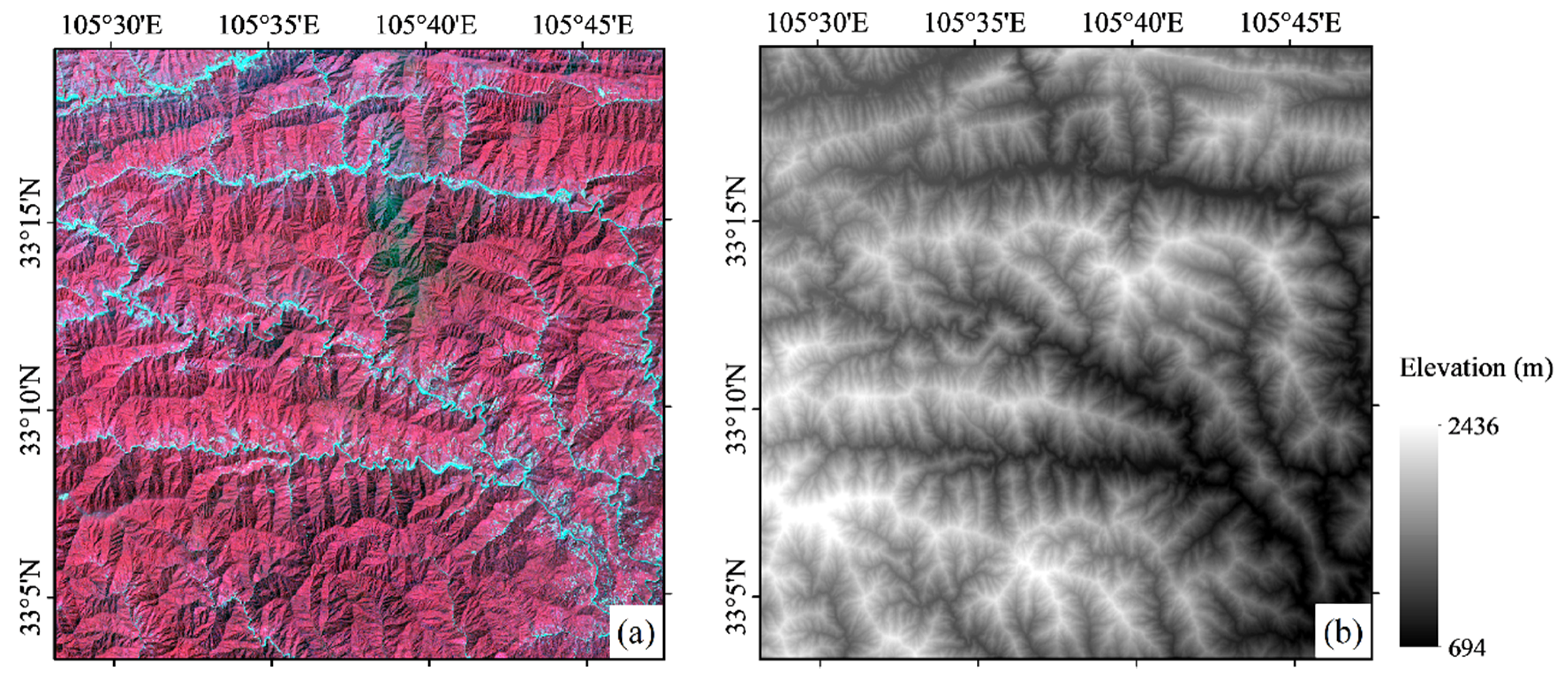
A 30 km × 30 km mountainous area centered at approximately 33°11.5′N, 105°38′E was selected as the study area (Figure 1a). The elevation varies from 694 m to 2436 m. The dominant land cover is broadleaved deciduous forest.

The Advanced Land Observing Satellite (ALOS) global digital surface model (AW3D30) dataset was used to calculate the slope and aspect, which are key parameters to implement topographic correction (Figure 1b). The spatial resolution is 1 arc-second (approximately 30 m). This dataset was generated through optical stereo matching of the Panchromatic Remote-sensing Instrument for Stereo Mapping (PRISM) images. AW3D30 was released on the website https://www.eorc.jaxa.jp/ALOS/en/aw3d30/data/index.htm by the Japan Aerospace Exploration Agency. An extensive validation activity revealed a height accuracy of 4.40 m (RMSE) [14], meeting the requirements of topographic correction [15].

The Sentinel-2A satellite carries a multispectral imager (MSI), covering 13 spectral bands. The spatial resolution is 10 m, 20 m and 60 m, depending on different bands. The revisit cycle of one satellite is 10 days. A cloud-free Sentinel-2A Level-1C image acquired on August 15, 2019 was downloaded from the Copernicus Open Access Hub (https://scihub.copernicus.eu). The solar zenith and azimuth angles were 25.09° and 134.16°, respectively. The Level-1C, i.e., top of atmosphere reflectance, Sentinel-2A images were atmospherically corrected using the Sen2Cor processor in the Sentinel Application Platform (SNAP) [16] to obtain the top of canopy reflectance. The terrain correction embedded in the recent Sen2Cor processor was not applied. The spatial resolution of Sentinel-2 was resampled to 30 m to be consistent with the AW3D30.

2.2. Vegetation Indices

Four VIs, i.e., NDVI, EVI, SAVI, and NIRv, were selected to test the topographic effects on VIs (

Table 1. Selected vegetation indices. NIR, R, and B are, respectively, the reflectances in the near-infrared, red, and blue bands.

Vegetation Index	Formula	Reference
NDVI	(NIR-R)/(NIR + R)	Tucker (1979) [2]
EVI	2.5(NIR-R)/(NIR + 6.0R − 7.5B + 1)	Huete et al. (2002) [3]
SAVI	1.5(NIR-R)/(NIR + R + 0.5)	Huete (1988) [4]
NIRv	NIR × NDVI	Badgley et al. (2017) [5]

). NDVI is the most widely used VI [2]; SAVI was designed to minimize soil effects [4]; EVI can reduce the saturation effect at high leaf area index values and is insensitive to atmospheric perturbation [3]; NIRv represents the near-infrared reflectance from vegetation and is more directly related to photosynthesis than more traditional VIs [5].

2.3. Topographic Normalization Methods

Many topographic correction methods exist in the literature (we refer to references [6,17,18,19] for detailed review and comparison). Three methods specifically designed to normalize topographic effects on surface reflectances were selected: SE [8], SCS + C [9], and PLC [12] (

Table 2. Formulas of selected topographic correction methods. $O_H$ and $O_t$ are remote sensing observations over horizontal and inclined surfaces, respectively. ${\overline{O}}_t$ is the mean of the $O_t$. A and B are slope and intercept of the linear regression between the observations and local illumination conditions, i (Equation (1)), respectively, and C is the ratio between A and B. ${\theta }_s$ and ${\phi }_s$ are solar zenith and azimuth angles, respectively. ${\theta }_v$ and ${\phi }_v$ are viewing zenith and azimuth angles, respectively. $\alpha$ and $\beta$ are slope and aspect of the terrain, respectively.

Method	Formula	Reference
SE	$O_H=O_t-\left(Acosi+B\right)+{\overline{O}}_t$	Teillet et al. (1982) [8]
SCS + C	$O_H=O_t\frac{cos \alpha cos {\theta }_s+C}{cos i+C}$	Soenen (2015) [9]
PLC	$O_H=O_t\frac{1/cos {\theta }_s+1/cos {\theta }_s\left(1-tan \alpha cos\left({\phi }_s-\beta \right)tan {\theta }_s\right)}{1/cos {\theta }_v+1/cos {\theta }_v\left(1-tan \alpha cos\left({\phi }_v-\beta \right)tan {\theta }_v\right)}$	Yin et al. (2018) [12]

). SE is an empirical method based on the regression relationship between reflectance and local illumination condition, $cos\left(i\right)$:

$$cos\left(i\right)=cos\left(\alpha \right)cos\left({\theta }_s\right)+sin\left(\alpha \right)sin\left({\theta }_s\right)cos\left({\phi }_s-\beta \right)$$

(1)

where $\alpha$ and $\beta$ are slope and aspect derived from DEM, respectively. ${\theta }_s$ and ${\phi }_s$ are solar zenith and azimuth angles, respectively [8,9]. SCS + C is also based on an empirical-statistical regression relationship between observations and $cos\left(i\right)$. SCS + C relies on the SCS method, which is derived from the simplification of a geo-optical model [10], and introduces an empirical parameter for the regulation of scattered radiation. The empirical parameters in both SCS + C and SE lack a physical basis. On the contrary, PLC has a solid physical basis and was derived from the solution to the canopy radiative transfer equation [12]. The underlying mechanism works so that the slope significantly distorts the angular distribution of the path length, which is a critical factor causing reflectance distortion [20,21]. Recent evaluation activities demonstrated that these three methods outperformed other existing methods [12,17,22].

We tested two alternative pathways to reduce the topographic effects on VIs: (1) firstly correct the topographic effects on reflectance, and then calculate VIs with the topographically corrected reflectance; and (2) calculate VIs with uncorrected reflectance, and then directly apply the topographic correction methods to the VIs. Herein, we refer to the two pathways as Correct-then-Index (CI) and Index-then-Correct (IC) strategies, respectively.

2.4. Evaluation Approach

Two criteria were used to assess the topographic effects on VIs before and after correction: (1) Correlation analysis: the correlation coefficient (R²) and the slope of the linear regression between the local illumination condition (Equation (1)) and the VIs; and (2) Aspect-dependence: the coefficient of variation (CV) (%) of the VI across different aspects. R², slope, and CV quantify the VIs’ variations caused by topography. The higher their values, the higher the topographic effects, and vice versa.

3. Results

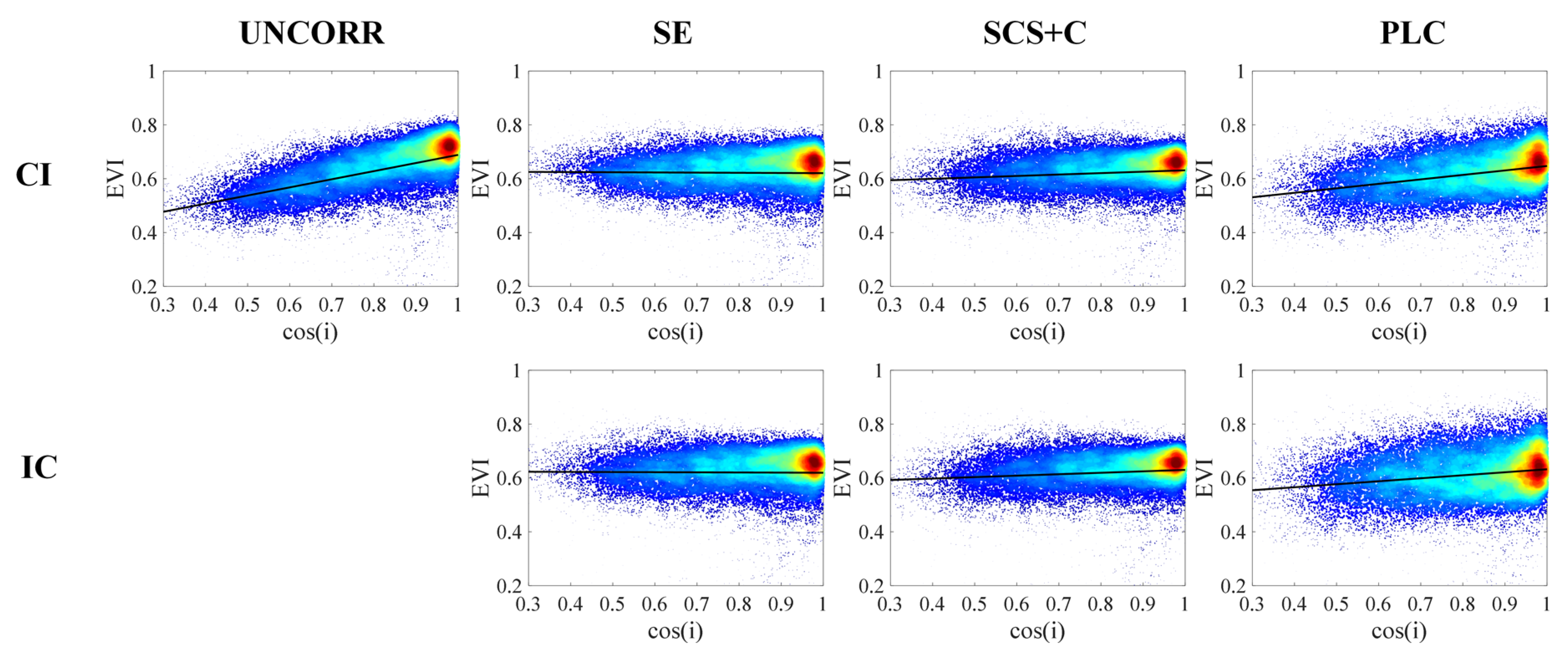
The statistics of the correlation analysis between VIs and local illumination conditions before and after the topographic correction with CI and IC strategies are presented in

Table 3. The slope and R² of the regression relationships between the local solar incidence angle and the normalized difference vegetation index (NDVI), the soil adjusted vegetation index (SAVI), EVI and the near-infrared reflectance of terrestrial vegetation (NIRv) before (un-corrected (UNCORR)) and after topographic correction (with SE, SCS + C and PLC methods). Lower values of the slope and R² of the linear regression indicate lower topographic effects. CI: first correct the topographic effects on reflectance, and then calculate vegetation index. IC: first calculate vegetation index, and then apply the topographic correction.

Method		NDVI		SAVI		EVI		NIRv
		Slope	R2	Slope	R2	Slope	R2	Slope	R2
UNCORR		−0.036	0.006	0.213	0.199	0.302	0.254	0.216	0.267
SE	CI	−0.006	0	−0.005	0	−0.007	0	−0.001	0
	IC	−0.001	0	−0.004	0	−0.005	0	−0.004	0
SCS + C	CI	−0.010	0.001	0.038	0.008	0.053	0.011	0.038	0.012
	IC	−0.008	0	0.038	0.009	0.054	0.012	0.036	0.011
PLC	CI	−0.036	0.006	0.114	0.058	0.166	0.080	0.115	0.078
	IC	−0.311	0.165	0.035	0.004	0.113	0.031	0.115	0.078

. For brevity, the relationships are shown only for the case of the EVI (Figure 2).

Topography-insensitive VIs should be characterized by values of R² and slope of the linear regression close to zero. The NDVI is insensitive to topographic effects (slope = −0.036, R² = 0.006). The EVI has the highest slope (0.302) and the NIRv has the highest correlation with illumination conditions (R² = 0.267). The topographic correction is not necessary for the NDVI and it may cause over-correction (after PLC correction with IC, the slope becomes −0.310). For the three non-normalized VIs, the topographic effects can be significantly reduced by both IC and CI. For example, the slope and R² between local illumination condition and EVI decrease from 0.302 and 0.254, respectively, to −0.005/0.050/0.110 and 0/0.010/0.031 after SE/SCS + C/PLC correction with IC strategy (see also Figure 2).

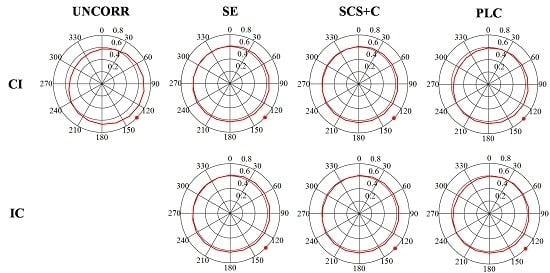
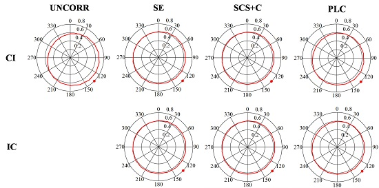
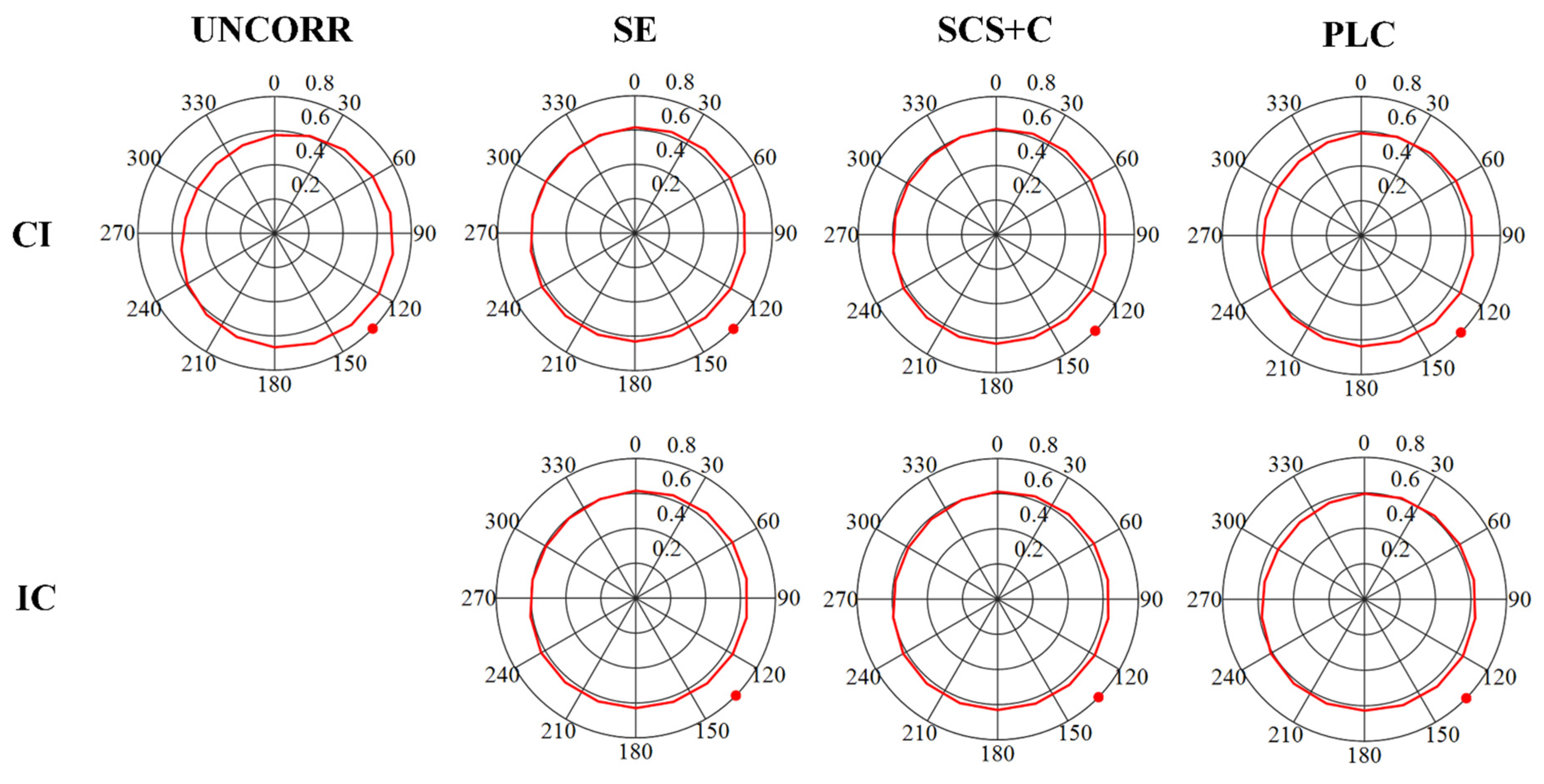
Figure 3 shows the EVI variations across different aspect angles. Before correction, the EVI over the sun-facing aspects was remarkably larger than those over the opposite directions, exhibiting significantly topographic influences. All the three topographic correction methods can obviously reduce the asymmetry of the EVI distribution across aspects, i.e., the topographic effects are successfully mediated.

Smaller values of the CV of VIs across different aspects indicate lower topographic effects, and vice versa.

Table 4. The coefficient of variation (%) of vegetation index across different aspects before (UNCORR) and after the topographic correction with SE, SCS + C, and PLC methods. CI: first correct the topographic effects on reflectance, and then calculate vegetation index. IC: first calculate vegetation index, and then apply the topographic correction.

Method		NDVI	SAVI	EVI	NIRv
UNCORR		0.66	8.13	10.46	14.07
SE	CI	1.03	2.16	2.53	3.55
	IC	1.04	2.22	2.59	3.38
SCS + C	CI	0.97	2.36	2.79	3.72
	IC	1.04	2.37	2.79	3.63
PLC	CI	0.66	4.51	5.87	7.76
	IC	6.33	1.95	4.16	7.76

presents the CV of VIs across different aspects before and after the topographic correction. Before correction, NDVI and NIRv have the smallest (0.66%) and largest CV (14.07%), respectively. For the three topography-sensitive VIs (EVI, SAVI, and NIRv), the CV is greatly reduced after the topographic correction using any correction methods (SE, SCS + C, or PLC) and strategies (CI or IC).

4. Discussion

We evaluated topographic effects through correlation analysis and aspect-dependence. We acknowledge that uncertainty exists in each of these two evaluation criteria. However, we analyzed the relationship of VIs and two complementary topographic indicators, i.e., local illumination condition and aspect; therefore, the combination of the two criteria can fully capture the topographic effects of the VIs and give a relatively objective result.

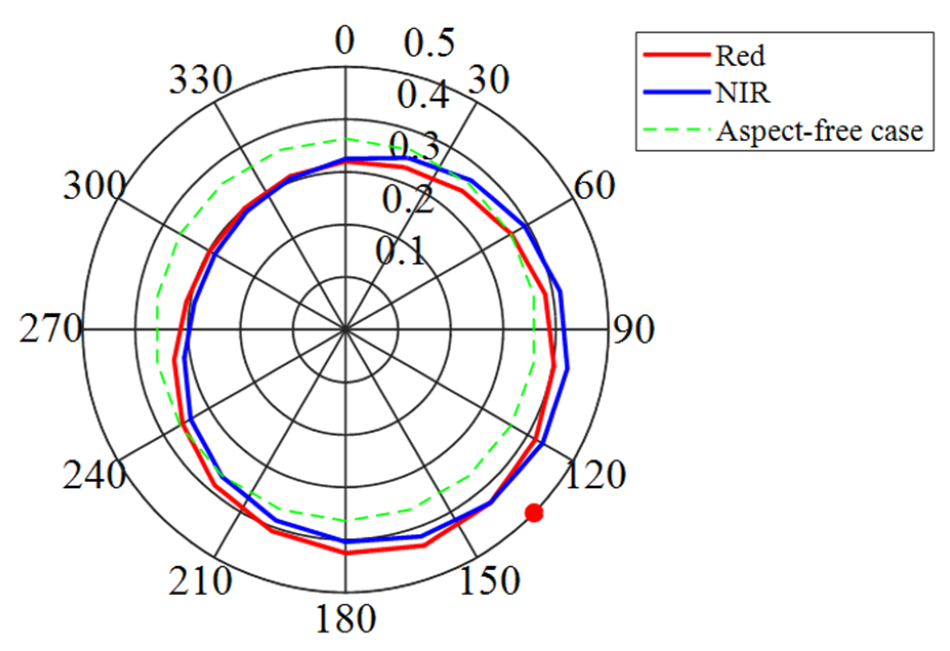
Results confirm previous findings on the fact that the NDVI is insensitive to topography [23,24,25]. Therefore, the topographic correction for NDVI appears unnecessary. The insensitivity of the NDVI to topography is attributed to the similar topographic influences in relative terms on the red and NIR spectral band reflectances, so the normalized band-ratio formula of NDVI can cancel out most of the topographic effects. To validate this assumption, we analyzed the reflectance distribution with aspect angles for both red and NIR bands (Figure 4). The two circles nearly overlap, with similar CV (13.3% and 14.2% for red and NIR bands, respectively). For visualization, the red band reflectance distribution was normalized such that it has an identical area to that of the NIR case.

However, NDVI suffers from saturation, background and atmospheric influences [3], and a wide number of alternative VIs, including the EVI, SAVI, and NIRv, were developed to cope with these uncertainties. This study reveals that the local illumination condition ($cos\left(i\right)$) can explain 19.85%, 25.37%, and 26.69% of the variation of the commonly used SAVI, EVI, and NIRv, respectively (see Table 3). It implies that although these alternative normalized VIs may outperform the NDVI in terms of soil and atmospheric dependences [26], topographic correction should be specially considered when applying them to mountainous areas.

The topographic correction for VIs is a long-neglected problem, and the very few existing related studies rely on the CI strategy, i.e., first correct reflectance and then calculate VIs. In this sense, Adhikari et al. [25] and Galvão et al. [27] found that the CI strategy can obviously reduce the correlation between non-normalized VIs and local illumination condition. Our study, for the first time, demonstrates the feasibility of directly applying topographic correction to VIs, i.e., IC strategy. Considering that high-level VI products, including bidirectional reflectance distribution function (BRDF) correction and other processing, are now freely accessed (e.g., MODIS EVI product [3]), our finding has important implications for their use in mountainous areas, because the topographic correction can be implemented by the end users of VIs through IC strategy.

An alternative approach is to develop novel VIs independent from topographic effects. Based on the finding that the soil adjustment factor in the EVI makes it very sensitive to topographic conditions [23], Liao et al. [28] modified the EVI by changing the soil adjustment index from a constant to a variable related to the incidence angle. This pioneering work provides a paradigm to extend the applicability of current VIs to mountainous areas. Forthcoming studies will explore these novel VIs insensitive to topography over more case studies and larger study areas.

5. Conclusions

We assessed the topographic effects on four VIs: NDVI, EVI, SAVI, and NIRv, calculated from Sentinel-2A. We corrected the topographic effects by three commonly used methods (SE, SCS + C, and PLC) through two strategies (CI and IC). The following two main conclusions were drawn:

• The NDVI is insensitive to topography, in agreement with the literature. On the contrary, EVI, SAVI, and NIRv need to be corrected from topographic effects over mountainous regions. Neglecting those effects, particularly for the recently developed NIRv, would cause prominent uncertainty for downstream applications.
• Existing topographic correction methods dedicatedly designed for reflectance can effectively reduce topographic effects on VIs. Besides the CI pathway, this study, for the first time, demonstrated the feasibility of directly applying SE, SCS + C, and PLC correction methods to VIs. This would significantly simplify the topographic correction process for VIs.

Our study will contribute to improved vegetation monitoring with VIs and benefit the retrieval of vegetation biophysical and biochemical parameters over mountainous areas. It is worth noting that the implementation of topographic correction methods for VIs through Google Earth Engine and other cloud platforms would substantially benefit the release of analysis-ready VI products.

References

- Huete, A.; Miura, T.; Yoshioka, H.; Ratana, P.; Broich, M. Indices of vegetation activity. In Biophysical Applications of Satellite Remote Sensing; Springer: Berlin/Heidelberg, Germany, 2014; pp. 1–41. [Google Scholar]
- Tucker, C.J. Red and photographic infrared linear combinations for monitoring vegetation. Remote Sens. Environ. 1979, 8, 127–150. [Google Scholar] [CrossRef] [Green Version]
- Huete, A.; Didan, K.; Miura, T.; Rodriguez, E.P.; Gao, X.; Ferreira, L.G. Overview of the radiometric and biophysical performance of the MODIS vegetation indices. Remote Sens. Environ. 2002, 83, 195–213. [Google Scholar] [CrossRef]
- Huete, A.R. A soil-adjusted vegetation index (SAVI). Remote Sens. Environ. 1988, 25, 295–309. [Google Scholar] [CrossRef]
- Badgley, G.; Field, C.B.; Berry, J.A. Canopy near-infrared reflectance and terrestrial photosynthesis. Sci. Adv. 2017, 3, e1602244. [Google Scholar] [CrossRef] [Green Version]
- Wen, J.; Liu, Q.; Xiao, Q.; Liu, Q.; You, D.; Hao, D.; Wu, S.; Lin, X. Characterizing Land Surface Anisotropic Reflectance over Rugged Terrain: A Review of Concepts and Recent Developments. Remote Sens. 2018, 10, 370. [Google Scholar] [CrossRef] [Green Version]
- Holben, B.; Justice, C. An examination of spectral band ratioing to reduce the topographic effect on remotely sensed data. Int. J. Remote Sens. 1981, 2, 115–133. [Google Scholar] [CrossRef]
- Teillet, P.M.; Guindon, B.; Goodenough, D.G. On the Slope-Aspect Correction of Multispectral Scanner Data. Can. J. Remote Sens. 1982, 8, 84–106. [Google Scholar] [CrossRef] [Green Version]
- Soenen, S.A.; Peddle, D.R.; Coburn, C.A. SCS + C: A modified sun-canopy-sensor topographic correction in forested terrain. IEEE Trans. Geosci. Remote Sens. 2005, 43, 2148–2159. [Google Scholar] [CrossRef]
- Gu, D.; Gillespie, A. Topographic normalization of landsat TM images of forest based on subpixel Sun-canopy-sensor geometry. Remote Sens. Environ. 1998, 64, 166–175. [Google Scholar] [CrossRef]
- Dymond, J.R.; Shepherd, J.D. Correction of the topographic effect in remote sensing. IEEE Trans. Geosci. Remote Sens. 1999, 37, 2618–2619. [Google Scholar] [CrossRef]
- Yin, G.F.; Li, A.N.; Wu, S.B.; Fan, W.L.; Zeng, Y.L.; Yan, K.; Xu, B.D.; Li, J.; Liu, Q.H. PLC: A simple and semi-physical topographic correction method for vegetation canopies based on path length correction. Remote Sens. Environ. 2018, 215, 184–198. [Google Scholar] [CrossRef]
- Yin, G.; Ma, L.; Zhao, W.; Zeng, Y.; Xu, B.; Wu, S. Topographic Correction for Landsat 8 OLI Vegetation Reflectances Through Path Length Correction: A Comparison Between Explicit and Implicit Methods. IEEE Trans. Geosci. Remote Sens. 2020, 1–13. [Google Scholar] [CrossRef]
- Tadono, T.; Nagai, H.; Ishida, H.; Oda, F.; Naito, S.; Minakawa, K.; Iwamoto, H. Generation of the 30 m-mesh global digital surface model by ALOS prism. In Proceedings of the XXIII ISPRS Congress, Prague, Czech Republic, 12–19 July 2016. [Google Scholar]
- Wu, Q.; Jin, Y.; Fan, H. Evaluating and comparing performances of topographic correction methods based on multi-source DEMs and Landsat-8 OLI data. Int. J. Remote Sens. 2016, 37, 4712–4730. [Google Scholar] [CrossRef]
- Main-Knorn, M.; Pflug, B.; Louis, J.; Debaecker, V.; Muller-Wilm, U.; Gascon, F. Sen2Cor for Sentinel-2. In Image and Signal Processing for Remote Sensing Xxiii; Bruzzone, L., Bovolo, F., Eds.; Spie-International Society Optical Engineering: Bellingham, WA, USA, 2017; Volume 10427. [Google Scholar]
- Sola, I.; González-Audícana, M.; Álvarez-Mozos, J. Multi-criteria evaluation of topographic correction methods. Remote Sens. Environ. 2016, 184, 247–262. [Google Scholar] [CrossRef] [Green Version]
- Hantson, S.; Chuvieco, E. Evaluation of different topographic correction methods for Landsat imagery. Int. J. Appl. Earth Obs. Geoinf. 2011, 13, 691–700. [Google Scholar] [CrossRef]
- Richter, R.; Kellenberger, T.; Kaufmann, H. Comparison of Topographic Correction Methods. Remote Sens. 2009, 1, 184–196. [Google Scholar] [CrossRef] [Green Version]
- Yin, G.; Cao, B.; Li, J.; Fan, W.; Zeng, Y.; Xu, B.; Zhao, W. Path Length Correction for Improving Leaf Area Index Measurements Over Sloping Terrains: A Deep Analysis Through Computer Simulation. IEEE Trans. Geosci. Remote Sens. 2020, 1, 1–17. [Google Scholar] [CrossRef]
- Yin, G.F.; Li, A.N.; Zhao, W.; Jin, H.A.; Bian, J.H.; Wu, S.B.A. Modeling Canopy Reflectance Over Sloping Terrain Based on Path Length Correction. IEEE Trans. Geosci. Remote Sens. 2017, 55, 4597–4609. [Google Scholar] [CrossRef]
- Hurni, K.; Van Den Hoek, J.; Fox, J. Assessing the spatial, spectral, and temporal consistency of topographically corrected Landsat time series composites across the mountainous forests of Nepal. Remote Sens. Environ. 2019, 231, 111225. [Google Scholar] [CrossRef]
- Matsushita, B.; Wei, Y.; Jin, C.; Onda, Y.; Qiu, G. Sensitivity of the Enhanced Vegetation Index (EVI) and Normalized Difference Vegetation Index (NDVI) to Topographic Effects: A Case Study in High-Density Cypress Forest. Sensors 2007, 7, 2636–2651. [Google Scholar] [CrossRef] [Green Version]
- Lyon, J.G.; Yuan, D.; Lunetta, R.S.; Elvidge, C.D. A change detection experiment using vegetation indices. Photogramm. Eng. Remote Sens. 1998, 64, 143–150. [Google Scholar]
- Adhikari, H.; Heiskanen, J.; Maeda, E.E.; Pellikka, P.K.E. The effect of topographic normalization on fractional tree cover mapping in tropical mountains: An assessment based on seasonal Landsat time series. Int. J. Appl. Earth Obs. Geoinf. 2016, 52, 20–31. [Google Scholar] [CrossRef]
- Kimm, H.; Guan, K.; Jiang, C.; Peng, B.; Gentry, L.F.; Wilkin, S.C.; Wang, S.; Cai, Y.; Bernacchi, C.J.; Peng, J.; et al. Deriving high-spatiotemporal-resolution leaf area index for agroecosystems in the U.S. Corn Belt using Planet Labs CubeSat and STAIR fusion data. Remote Sens. Environ. 2020, 239, 111615. [Google Scholar] [CrossRef]
- GalvãO, L.S.; Breunig, F.M.; Teles, T.S.; Gaida, W.; Balbinot, R. Investigation of terrain illumination effects on vegetation indices and VI-derived phenological metrics in subtropical deciduous forests. Mapp. Sci. Remote Sens. 2016, 53, 360–381. [Google Scholar]
- Liao, Z.M.; He, B.B.; Quan, X.W. Modified enhanced vegetation index for reducing topographic effects. J. Appl. Remote Sens. 2015, 9, 96068. [Google Scholar] [CrossRef]
Figure 1.
Study area. (a) Sentinel-2A image from August 15, 2019 (the R, G, and B color space correspond to bands 8A (narrow NIR), 4 (red), and 3 (green), respectively). (b) Elevation map from AW3D30.
Figure 2.
Density scatterplots between the enhanced vegetation index (EVI) and the cosine of the local solar incidence angle () with statistical-empirical (SE), sun-canopy-sensor with C-correction (SCS + C), and path length correction (PLC) methods through Correct-then-Index (CI) strategy (first correct the topographic effects on reflectance, and then calculate vegetation index) and Index-then-Correct (IC) strategy (first calculate the VI and then apply the topographic correction methods).
Figure 3.
Mean EVI distribution with aspect angles before (UNCORR) and after topographic correction with SE, SCS + C, and PLC methods through CI strategy and IC strategy. The polar angle represents the aspect, and the radius represents the magnitude of the EVI with zero in the center. The red point represents the sun azimuth angle at 134.16°.
Figure 4.
Mean reflectance distribution with aspect angles. The polar angle represents the aspect, and the radius represents the magnitude of the reflectance with zero in the center. The red point represents the sun azimuth angle. The blue and red circles represent NIR and red bands, respectively. For visualization, the red band reflectances were normalized such that it has an identical area to that of NIR reflectances. The dashed green circle is the hypothetically aspect-free case whose radius is the averaged value of the UNCORR reflectances across different aspects and centered in the ordinate origin.