Estimating River Sediment Discharge in the Upper Mississippi River Using Landsat Imagery

Abstract

With the decline of operational river gauges monitoring sediments, a viable means of quantifying sediment transport is needed. In this study, we address this issue by applying relationships between hydraulic geometry of river channels, water discharge, water-leaving surface reflectance (SR), and suspended sediment concentration (SSC) to quantify sediment discharge with the aid of space-based observations. We examined 5490 Landsat scenes to estimate water discharge, SSC, and sediment discharge for the period from 1984 to 2017 at nine gauging sites along the Upper Mississippi River. We used recent advances in remote sensing of fluvial systems, such as automated river width extraction, Bayesian discharge inference with at-many-stations hydraulic geometry (AMHG), and SSC-SR regression models. With 621 Landsat scenes available from all the gauging sites, the results showed that the water discharge and SSC retrieval from Landsat imagery can yield reasonable sediment discharge estimates along the Upper Mississippi River. An overall relative bias of −25.4, mean absolute error (MAE) of 6.24 × 10⁴ tonne/day, relative root mean square error (RRMSE) of 1.21, and Nash–Sutcliffe Efficiency (NSE) of 0.49 were obtained for the sediment discharge estimation. Based on these statistical metrics, we identified three of the nine gauging sites (St. Louis, MO; Chester, IL; and Thebes, IL), which were in the downstream portion of the river, to be the best locations for estimating water and sediment discharge using Landsat imagery.

1. Introduction

Rivers are vital components of a drainage basin. They act as habitats for aquatic organisms, serve as drainage channels for surface water, and regulate the hydrological cycle. They provide water for domestic, industrial and agricultural use, power generation, and navigation [1,2]. Anthropogenic activities have increasingly altered rivers’ physical and chemical properties [3,4,5,6]. These activities include agricultural practices, industrial operations, and land use and land cover changes, which all tend to negatively impact surface water quality through excessive point- or nonpoint-source loadings of pollutants [3,7,8,9,10,11]. A major driver of this problem is human-induced sedimentation, which affects the hydrologic regime and water quality of a river and its drainage basin [12,13,14]. Human activities, such as agriculture, forest operations, mining, and urbanization, increase erosion and sediment transport within a drainage basin [15].

Under natural conditions, sediment transport in rivers helps in carrying soil towards floodplains, delivering nutrient-rich soils to improve the agricultural productivity of adjacent lands. Changes in sediment transport impact fluvial properties and processes, such as geochemical cycling, channel morphology, and delta development [15]. In recent decades, anthropogenic activities have changed sedimentation across the globe, in both increasing and decreasing trends [16]. Martinez et al. [17] reported that global changes in rainfall patterns and regional land cover changes have led to an increase in sediment transport in the Amazon River. In contrast, Wang et al. [18] reported a marked decrease in sedimentation in the Yellow River due to vegetation restoration and construction of sediment trapping systems such as dams and reservoirs. Both scenarios have been reported for the Mississippi River [19,20,21,22]. A gradual increase in sedimentation has been estimated beginning with European settlement in 1830 due to the introduction of forest clearance and tillage practices, and continuing with a sharp increase between 1940 and 1970, likely caused by the rise of agricultural and industrial activities [19]. Holeman [20] estimated that, during 1951–1965, the Mississippi River’s sediment discharge averaged 3.12 × 10⁸ tonnes (t) annually. A subsequent report by Milliman and Meade [21] indicated that yearly sedimentation in the Mississippi River had declined to 1.91 × 10⁸ t during 1963–1979 due to reservoir and dam construction, the implementation of measures to control river bank erosion, and improved soil conservation practices within the drainage basin. A later study by Meade and Moody [22] reported a continued trend of decreasing sedimentation in the river system, with an average annual sediment yield of 1.32 × 10⁸ t between 1986 and 2007. The authors suggest that the decrease was due to the reduced sediment supply upstream owing to the installation of sediment trapping structures and soil conservation practices.

Gauging stations and hydrologic models are widely used to measure and estimate sediment transport. Gauging stations are instrumented to directly measure river properties such as water discharge and sediment concentration at a site; these properties are then used to estimate sediment transport. In the US, sediment transport is commonly reported as sediment discharge, which represents the suspended sediment load across the river and is calculated based on field-measured, time-weighted discharge and suspended sediment concentration (SSC) [23,24]. At the watershed or regional scale, sediment transport can be assessed using hydrologic models [25,26], which require information about key watershed properties, such as topography, climate, soil, and vegetation [27,28]. These models are highly dependent upon the availability of input data. In data-scarce regions, representation of physical properties and processes as model inputs poses a challenge.

Numerous studies have assessed hydrologic processes and water quality parameters in rivers via space-based observations. These processes and parameters include floodplain water storage in braided rivers, inundation extent, stage variation, ice cover, turbidity, chlorophyll a, and flood wave propagation [29,30,31,32,33,34,35,36]. These studies demonstrated the potential of monitoring rivers from space on a broad scale as well as in cases where the study river is in a data-scarce region. River discharge, a critical property, was also estimated recently with optical satellite data. Gleason and Smith [37] submitted that the at-a-station hydraulic geometry (AHG) parameters (site-specific coefficients and exponents statistically relating river width to discharge) are related across all cross-sections within the same river, and therefore referred to such relationships as at-many-stations hydraulic geometry (AMHG). AMHG allows reach-averaged discharge to be estimated solely by hydraulic geometry, which is especially useful where river cross-sectional widths can be extracted from satellite data, such as Landsat, Sentinel-2, or Cubesat imagery [38]. Hagemann et al. [39] further developed the AMHG discharge estimation method using a Bayesian inference approach. The Bayesian-AMHG method uses prior information on AHG parameters and discharge data from various sources, e.g., literature, in situ measurements, and reanalysis datasets [38,39]. Given the wide coverage of remotely sensed data, there is potential for using the AMHG approach for discharge estimation across river basins, especially for regions where gauging stations are limited or non-existent.

Only a few studies have attempted to estimate sediment discharge via remotely sensed data [17,40,41,42]. These studies used field-measured water discharge and estimated the sediment concentration using remotely sensed water-leaving reflectance (usually with 250-m MODIS (Moderate Resolution Imaging Spectroradiometer) data) to determine the sediment discharge. A related study also explored using satellite gravimetry to estimate the sediment discharge of major rivers to the ocean [43]. More commonly, river sedimentation estimates from remotely sensed data are reported in terms of suspended sediment concentration along a river reach, or volume of sediment deposition at the river deltas or coastal zones [44,45,46,47,48,49,50,51,52]. In the former, SSC is estimated through empirical relationships between the remotely sensed surface reflectance (SR) of sampling areas and field-measured SSC. In the latter, the volume of sediment deposition is determined using channel change detection from digital elevation models constructed from laser altimetry and image processing.

Over the next decades, land surface changes will continue to contribute to changes in terrestrial sedimentation. Nonetheless, despite the increasing demands for sediment data [53], there has been an evident decline and discontinuation of operational gauging stations in many areas across the US. Monitoring operations may be hampered by accuracy requirements, cost, and safety concerns over traditional labor-intensive field sampling methods. There is a need for alternative approaches for the continuous monitoring of our river systems. With recent advancements in remote sensing of rivers, the use of space-based observations could offer greater opportunities to address the need. A method using remotely sensed information also allows us to compare rivers without gauging stations and identify which rivers have higher sedimentation rates than others.

This study was undertaken to investigate the potential of estimating sediment discharge using remotely sensed data, as an alternative method for providing useful hydrological information at lower cost. Specifically, we: (1) developed a method for estimating river sediment discharge from Landsat imagery, and applied it to nine gauging sites in the Upper Mississippi River; (2) established relationships between suspended sediment concentration and Landsat surface reflectance; and (3) evaluated the predictive performance of the approach for sediment discharge estimation against field-measured sediment data from United States Geological Survey (USGS) gauging stations.

2. Materials and Methods

2.1. Study Sites and Data

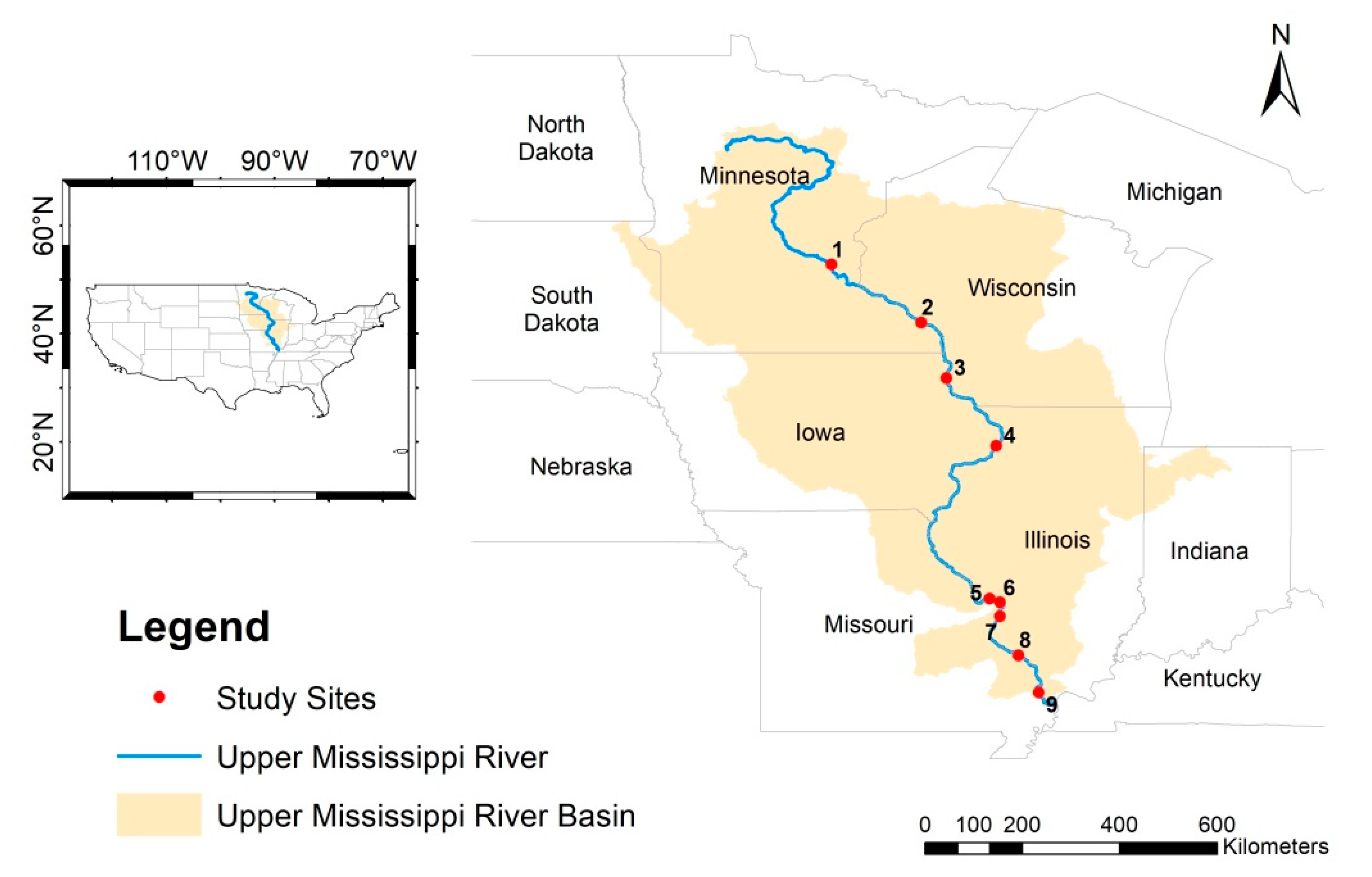
The research area for this study was the Upper Mississippi River, which stretches approximately 2100 km and composes nearly half of the entire Mississippi River. The main tributaries include the Missouri, Illinois, Wisconsin, and Iowa rivers. Three national wildlife refuges are present within the Upper Mississippi River Basin, which supports over 120 species of fish and 300 migratory bird species [54]. The USGS has installed 43 gauging stations to monitor the quantity and quality of water in the Upper Mississippi River, and daily flow and sediment discharge records are available in the USGS database for the period from 1861–2017. Of these 43 stations, nine have simultaneous records of daily flow and sediment discharge. This study examined all nine of these gauging stations (hereafter study sites) for the estimation of sediment discharge (Figure 1).

The nine study sites are located in four different states, namely Minnesota, Iowa, Illinois, and Missouri, with varying periods of available flow and sediment records (

Table 1. General information and periods of available flow and sediment data (both suspended sediment concentration (SSC) and sediment discharge) for the nine Upper Mississippi River study sites shown in Figure 1. Source: https://waterdata.usgs.gov/nwis/.

Site	Longitude	Latitude	USGS Gauge ID	Location	Flow Data	Sediment Data
1	−93.30	45.13	05288500	Brooklyn Park, MN	1931–present	1975–1996
2	−91.64	44.06	05378500	Winona, MN	1928–present	1975–1988
3	−91.17	43.03	05389500	McGregor, IA	1936–2013	1975–2004
4	−90.25	41.78	05420500	Clinton, IA	1873–present	1994–1997
5	−90.37	38.95	05587455	Grafton, IL	1997–present	1989–2017
6	−90.18	38.89	05587500	Alton, IL	1933–1987	1982–1989
7	−90.18	38.63	07010000	St. Louis, MO	1861–present	1980–2017
8	−89.84	37.90	07020500	Chester, IL	1942–present	1982–2017
9	−89.47	37.22	07022000	Thebes, IL	1933–present	1982–2017

). Among these sites, the earliest flow data were recorded at St. Louis, MO, in 1861, and monitoring has continued until the present. The earliest sediment monitoring was started in 1975 at the gauging stations of Brooklyn Park, MN; Winona, MN; and McGregor, IA, followed by other operations in the 1980s. Most USGS gauging stations have remained operational and still record water discharge. However, most sediment monitoring efforts have been halted, with the last data at St. Louis, MO; Grafton, IL; Chester, IL; and Thebes, IL, being recorded on 30 September 2017.

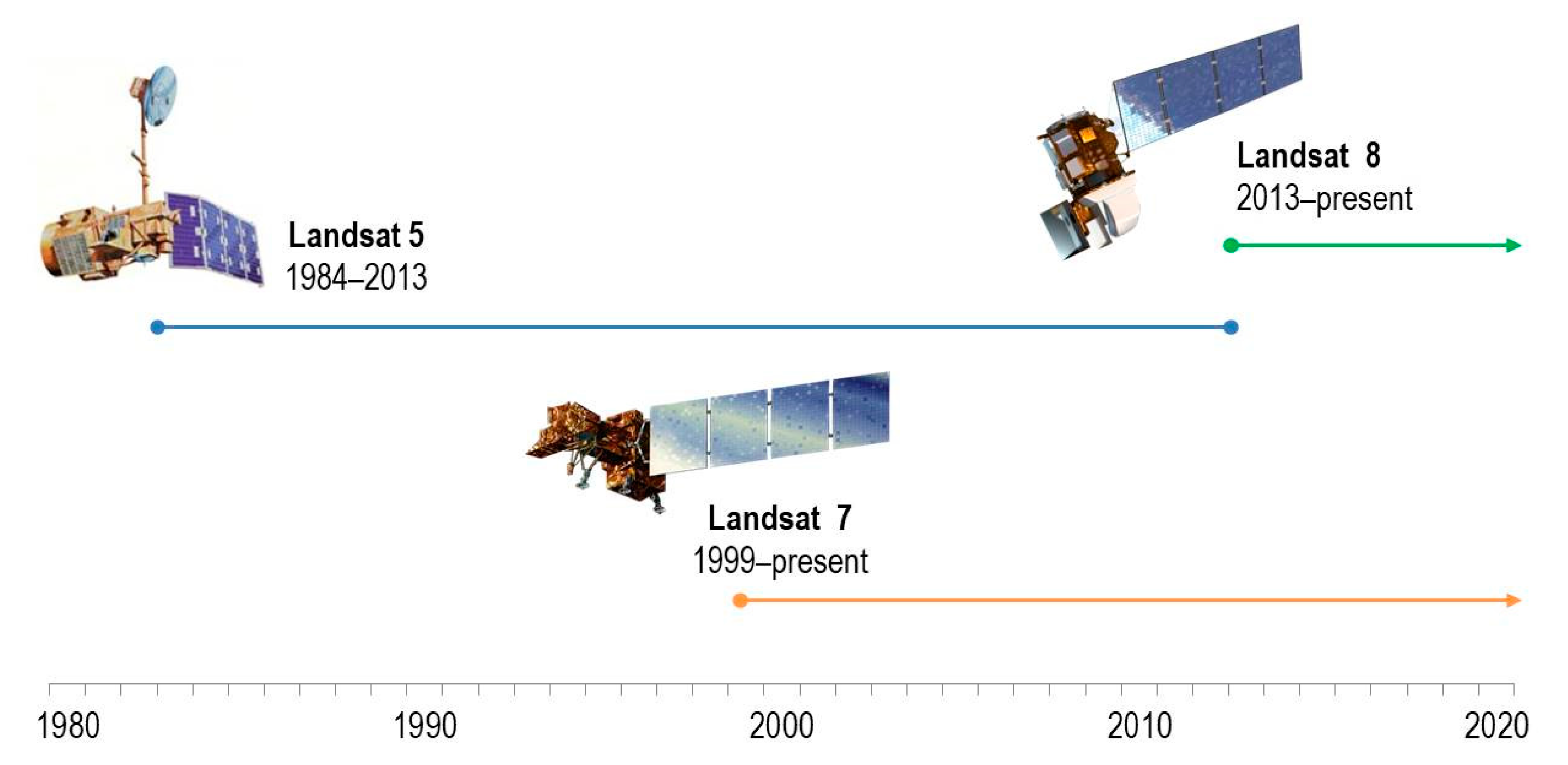
To estimate sediment discharge using remotely sensed data, we inspected the availability of remotely sensed imageries for three Landsat missions (5, 7, and 8) with different periods of operation in orbit (Figure 2). Landsat 5 captured Earth images with a thematic mapper (TM) sensor from March 1984 to January 2013, when it was decommissioned. Landsat 7 started its mission in 1999 and is presently operational with its enhanced thematic mapper plus (ETM+) sensor. However, since May 2003, it has been adversely impacted by a failure of the scan line corrector. Landsat 8 was launched as the Landsat Data Continuity Mission with the Operational Land Imager (OLI). It began capturing Earth images in 2013 and remains operational.

These Landsat missions share a common temporal resolution of 16-day repeat coverage, and 30-m spatial resolution for visible, near-infrared, and shortwave infrared bands. Multi-temporal Tier 1 Landsat scenes (pre-processed Landsat data at the highest available quality) were compiled using the Google Earth Engine platform [55], which allows a user to directly visualize, sort, and process imagery within the cloud platform. We identified 5490 Landsat scenes from March 1984 to September 2017 for which corresponding sediment data were available at the nine study sites in the Upper Mississippi River (

Table 2. Available Landsat images (5490 total) with corresponding sediment data for the Upper Mississippi River study sites.

Site	Location	Flow and Sediment Data	Landsat Acquisition Path/Row	Number of Landsat Images
				Landsat 5	Landsat 7	Landsat 8	Total
1	Brooklyn Park, MN	1975–1996	27/29	141	-	-	141
2	Winona, MN	1975–1988	25/29, 25/30, 26/29	175	-	-	175
3	McGregor, IA	1975–2004	25/30	286	80	-	366
4	Clinton, IA	1994–1997	24/31, 25/31	93	-	-	93
5	Grafton, IL	1989–2017	23/33, 24/33	636	609	117	1362
6	Alton, IL	1982–1989	23/33, 24/33	142	-	-	142
7	St. Louis, MO	1980–2017	23/33, 24/33	786	609	180	1575
8	Chester, IL	1982–2017	22/34, 23/34, 24/34	403	317	88	808
9	Thebes, IL	1982–2017	23/34	418	323	87	828

(-) no data

). Some study sites share similar Landsat acquisition path/row numbers (e.g., Grafton, IL; Alton, IL; and St. Louis, MO, at 23/33), meaning that they had similar nominal scene centers.

2.2. River Discharge Estimation using Landsat Imagery

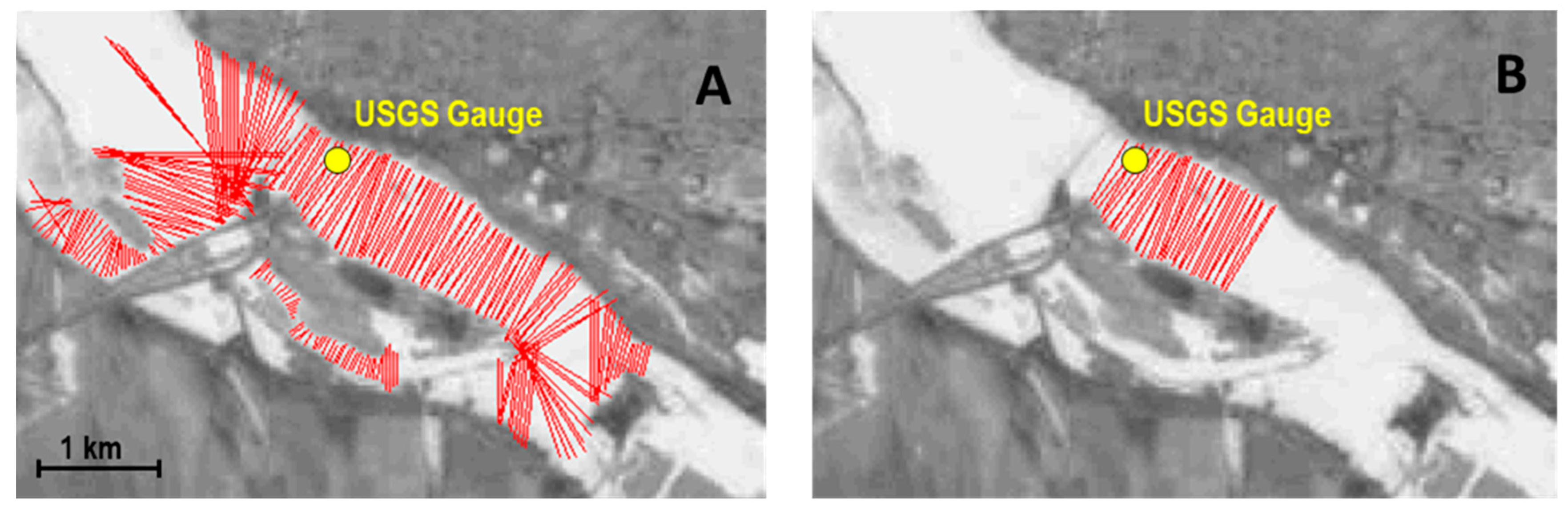
River widths obtained from Landsat river masks were used as inputs for the river discharge retrievals. Prior to width extraction, the imagery collection for each site was filtered to obtain those with less than 10% cloud obstruction at the gauging site. The cross-sectional widths along the river channels were extracted using the RivWidthCloud algorithm in Google Earth Engine following Yang et al. [56]. RivWidthCloud automatically extracts the centerline and width transects from the river mask of the area of interest in the Landsat imagery. The algorithm also detects widths obstructed due to clouds, cloud shadows, and snow. The resulting river widths were visually inspected and filtered to retain only those having midpoints within a ~1-km distance from their respective USGS gauging site (Figure 3), so as to best represent the reach of their site. In addition, widths within the standing confluence at an individual study site were excluded. The filtered river widths were subsequently used as inputs for the Bayesian-AMHG inference of river discharge.

The Bayesian-AMHG [37,39] was developed based upon the classic relationship between the hydraulic geometry of river channels and river discharge. Leopold and Maddock [57] posited a power-law statistical relationship between a river’s width and discharge:

W = aQ^b

(1)

where W is the river’s width, Q is its discharge, and a and b are the classic AHG parameters. For an AMHG relationship, the AHG parameter a is substituted by the AMHG parameters, and the discharge equation becomes:

$$Q={\left(\frac{W_{\mathrm{i}}}{W_{\mathrm{c}}}\right)}^{\frac{1}{b_{\mathrm{i}}}}{ Q}_{\mathrm{c}}$$

(2)

where W_c and Q_c are global AMHG parameters, and W_i and b_i are, respectively, the river width and the classic AHG parameter for each river cross section [37,39]. Equation (2) is the basis for the inference of river discharge in the Bayesian-AMHG method.

Bayesian inference requires both the likelihood of data and prior probability distributions of unknown parameters in order to obtain the full posterior distribution via Monte Carlo sampling [39]. Log-transforming Equation (2) yields a likelihood function and the prior probability distributions of the unknown parameters (b_i, W_c, Q_c, and Q). Based on a large number of acoustic doppler current profiler (ADCP) measurements at 10,081 USGS gauging stations, Hagemann et al. [39] obtained the likelihood function:

log W_i = b_i (log Q – log Q_c) + log W_c + ε

(3)

where ε is the AMHG error term with a standard deviation (SD) of 0.22. The prior distributions for Q and Q_c both follow a truncated normal distribution with a coefficient of variation of 1. The empirical prior distribution of the AHG parameter b, which is normally distributed, is given by:

log b = 0.02161 + 0.4578 SD (log W) + ε_b

(4)

where ε_b is the random error with a standard deviation of 0.098. Further, the prior distribution of W_c is log-normally distributed with its center at the mean width observed for the river reach, with a coefficient of variation of 0.01. From these likelihood and prior distributions, 1000 realizations of the posterior distribution were generated via Monte Carlo sampling, and a mean expected value of river discharge was obtained for each image [39].

We explored the sensitivity of the posterior mean value of Q to the prior distribution through the use of three different central tendency metrics. Following Feng et al. [38], we examined the potential of discharge estimation for gauged and ungauged settings. Three centers of distribution were analyzed, specifically, the median of daily discharge records Q_median from the USGS database (gauged rivers) and two empirical water balance model mean discharges (Q_wbm1 and Q_wbm2) obtained from widths extracted for each study site (ungauged rivers). For the ungauged rivers, we developed an empirical power-law function to estimate mean discharge based solely on the widths obtained from Landsat imagery. Through reanalysis of widths and water balance model-based mean discharge for 34 independent rivers across the globe compiled by Hagemann et al. [39], we obtained this function:

$$Q_{wbm1}=0.1813 {\overline{W}}^{1.4691}$$

(5)

where Q_wbm1 is the mean discharge from the first empirical water balance model and $\overline{W}$ is the mean width extracted for the study site (see Supplemental files, Figure S1). Q_wbm2 is the mean discharge from the second empirical water balance model obtained by doubling Q_wbm1. This additional empirical metric was included to explore how doubling a center of distribution for Q prior affects the final discharge estimate.

2.3. Estimating Suspended Sediment Concentration

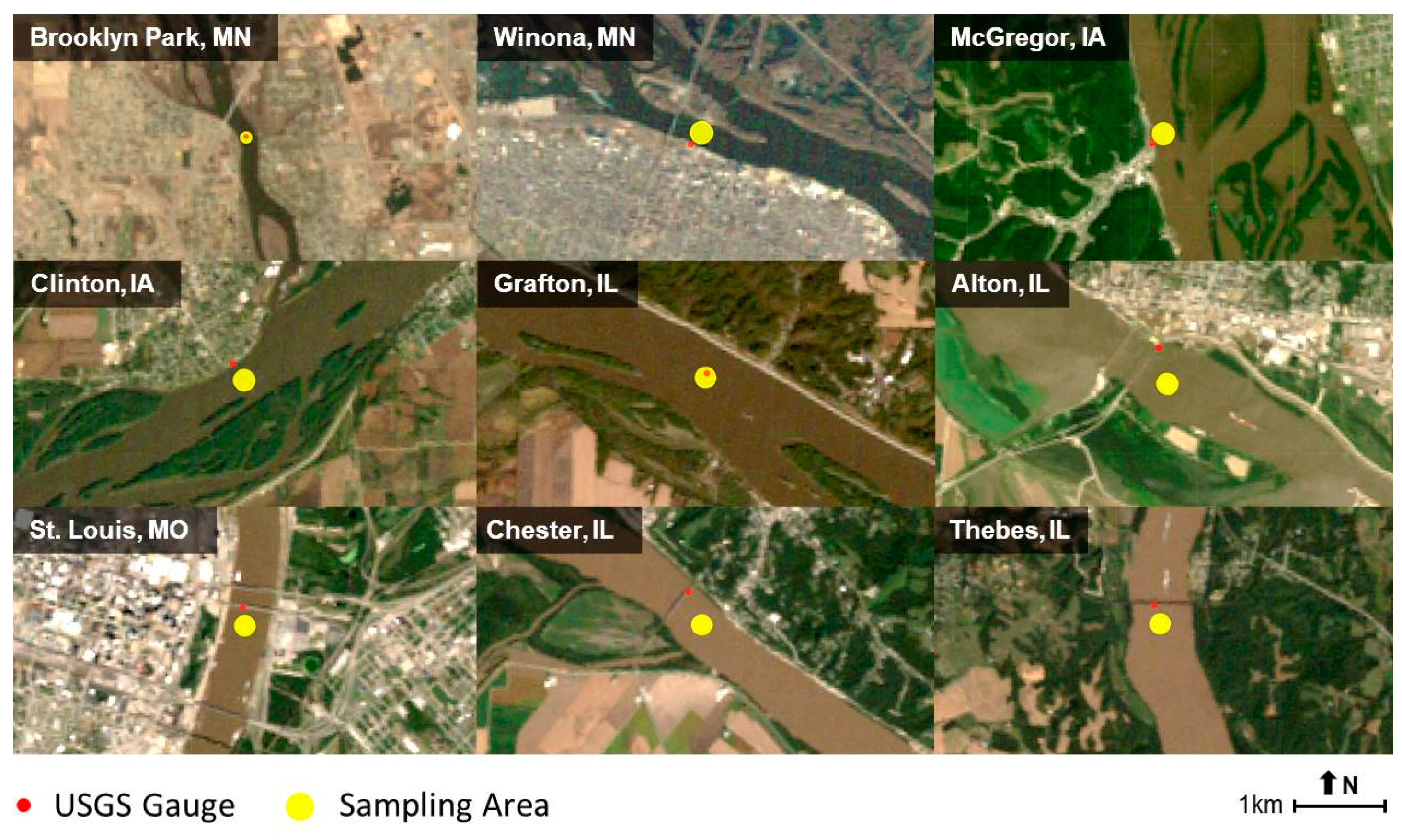
To estimate the SSC at the study sites, we fit the relationship between SSC and surface reflectance (SR) of Landsat images using a different set of images from those used in the discharge retrieval (see Supplemental files, Table S1). Using different image sets allowed an independent performance assessment of SSC and sediment discharge estimation. We identified and obtained the corresponding standard Landsat SR data, which were pre-processed using specialized atmospheric correction methods. The standard Landsat SR was generated from the Landsat Ecosystem Disturbance Adaptive Processing System (LEDAPS) for Landsats 5 and 7, and from the Surface Reflectance Code (LaSRC) for Landsat 8. Using Google Earth Engine, we applied a water mask for all Landsat imagery to identify for each study site a sampling area (diameter 240 m, except for study site 1 for which a radius of 120 m was used) that was at the center of the river reach, near the USGS gauge location, and clear of obstructions (e.g., bridges, ports, etc.) (Figure 4). Mean surface reflectance within the sampling area was calculated for each available Landsat image.

Related studies reported a correlation between SSC and the ratio of red band (0.63–0.69 µm: Band 3 for Landsat 5 and 7, Band 4 for Landsat 8) to green band (0.52–0.60 µm: Band 2 for Landsat 5 and 7, Band 3 for Landsat 8) reflectance in Landsat imagery. This correlation was adopted for this study given the reasonable goodness of fit (R² > 0.5) [48,49,50,51]. Regression functions relating SSC and SR were developed using the in situ SSC measurements and the water-leaving red to green reflectance ratio for each of the specified sampling areas of the nine gauging stations, and for the Upper Mississippi River as a whole using the pooled data. A total of 1854 scenes with corresponding SSC data were used to develop the gauge-specific and the regional-scale regressive SSC-SR functions (for a detailed image count at each study site, see Supplement file, Table S1). These functions were then applied to a set of 621 Landsat images (1) that were successfully used for river discharge estimation, and (2) for which USGS sediment data were available to estimate the mean SSC from surface reflectance. We assume that the estimated mean SSCs are also representative of the channel depth as the in situ SSC measurement of the USGS follows the sampling techniques described by Edwards and Glysson [58]. Accordingly, this set of images with estimated Q and SSC was used for the final sediment discharge estimation.

2.4. Sediment Discharge Estimation and Performance Evaluation

The relationship between river sediment discharge, river discharge, and SSC is described by Porterfield [23] as:

Q_s = k × Q × SSC

(6)

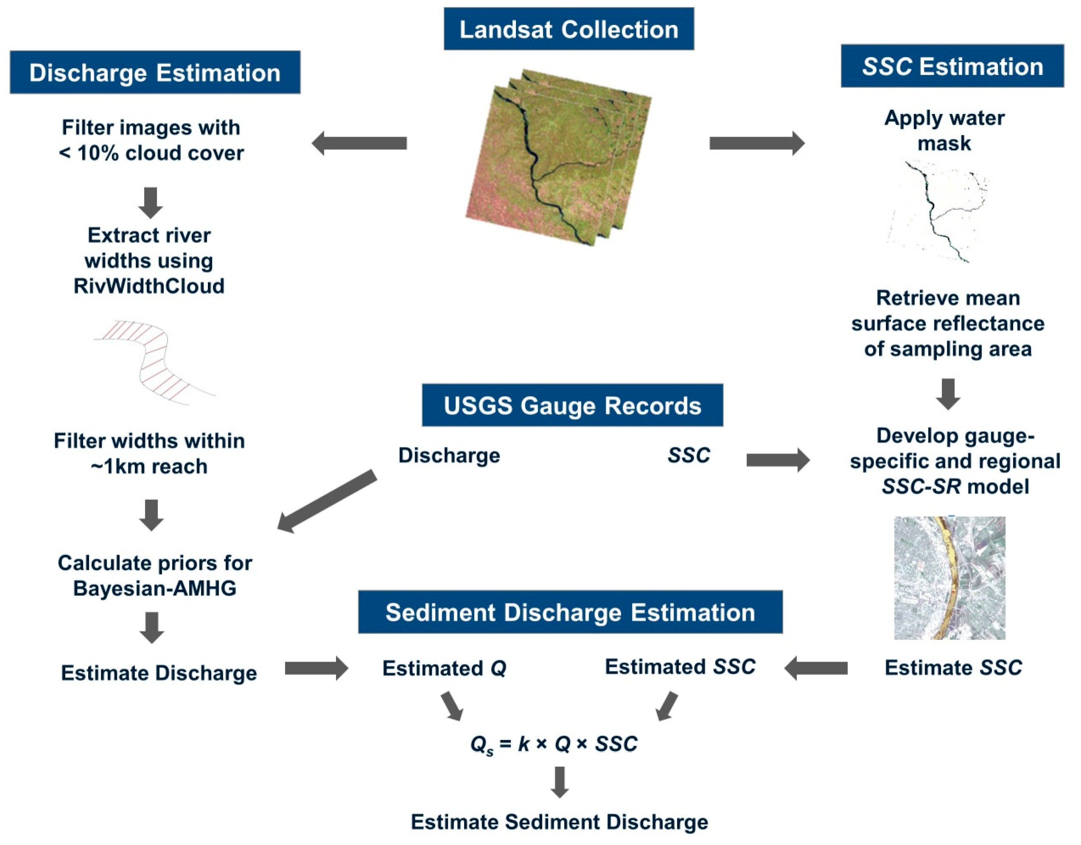
where Q_s is the sediment discharge (t/d), Q is the river discharge (m³/s), SSC is the mean suspended sediment concentration (mg/L), and k is a coefficient based on the units of the river discharge that assumes a specific weight of 2.65 for sediment (0.0864 in SI units). We applied this relationship to obtain sediment discharges for each gauging station. Figure 5 summarizes the main steps to estimate river sediment discharge based on Landsat imagery.

We evaluated the predictive performance of our approach to estimate river discharge, SSC, and sediment discharge for the study sites in the Upper Mississippi River with the set of 621 Landsat images from 1984 to 2017. Four statistical indicators, the Nash–Sutcliffe Efficiency (NSE), relative bias, mean absolute error (MAE), and the relative root mean square error (RRMSE), were calculated following Equations (7)–(10):

$$NSE=1-\frac{{{\displaystyle \sum }}_{\mathrm{i}=1 }^N{\left(y_i-{ y}_i^{\prime }\right)}^2}{{{\displaystyle \sum }}_{\mathrm{i}=1}^N {\left(y_{i }-\overline{y}\right)}^2}$$

(7)

$$Relative bias=\frac{\frac{1}{N}{{\displaystyle \sum }}_{\mathrm{i}=1 }^{\mathrm{N}}\left({ y}_i^{\prime }-{ y}_i\right)}{\overline{y}}$$

(8)

$$MAE=\frac{1}{N} {\displaystyle \sum }_{\mathrm{i}=1 }^N\left|y_{\mathrm{i}}-{ y}_{\mathrm{i}}^{\prime }\right|$$

(9)

$$RRMSE=\frac{1}{\overline{y}} \sqrt{\frac{{{\displaystyle \sum }}_{\mathrm{i}=1 }^N{\left(y_i-{ y}_i^{\prime }\right)}^2}{N}}$$

(10)

where y_i is the observed value (discharge, SSC, and sediment discharge), y_i’ is the estimated value, ȳ is the average of the observed values, and N is the number of observations.

3. Results

3.1. River Widths and Landsat Surface Reflectance Retrieval

Out of 5490 Landsat images available for the nine study sites (Table 2), 779 yielded river widths through the use of RivWidthCloud and post-processing techniques (

Table 3. Statistics of river widths obtained from Landsat imagery for the nine study sites.

Site	Location	N	Minimum	Maximum	Mean (m)	SD (m)	CV (%)
			(m)	(m)
1	Brooklyn Park, MN	34	81.0	181.8	121.8	17.2	14.1
2	Winona, MN	24	124.1	326.2	237.3	29.8	12.6
3	McGregor, IA	99	175.1	390.8	273.4	28.1	10.3
4	Clinton, IA	37	335.5	565.1	445.7	51.3	11.5
5	Grafton, IL	107	657.4	1337.5	947.6	98.9	10.4
6	Alton, IL	22	571.8	982.1	755.8	68.8	9.1
7	St. Louis, MO	121	300.8	641.6	452.4	48.3	10.7
8	Chester, IL	166	300.7	761.2	552.8	67.5	12.2
9	Thebes, IL	169	403.8	908.5	637	72.3	11.4

). The narrowest river channel, 121.8 m at Brooklyn Park, MN, was at the study site farthest upstream. The widest river channel, 947.6 m, was at Grafton, IL, toward the middle of the Upper Mississippi River. An advantage of automating the image-based width extraction is the consistency of width delineation from the river water mask, as seen in the similar coefficient of variation (CV) values. Such consistency reduces the uncertainty that would have been incurred by manually delineating river widths from remotely sensed images.

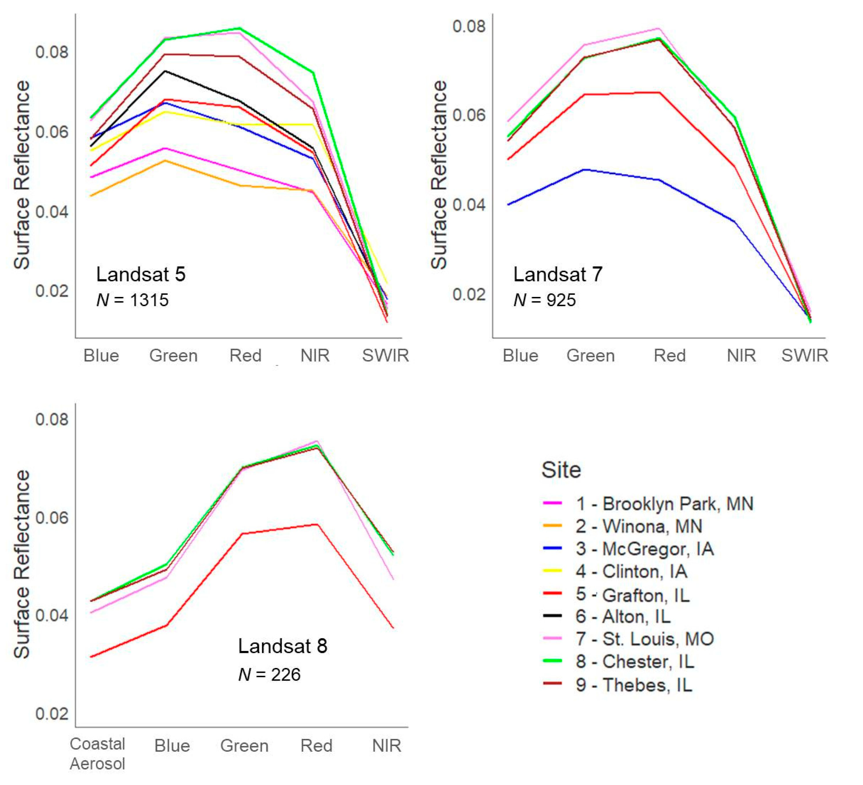
From the same pool of 5490 images, those lacking either reflectance values in the sampling areas or corresponding sediment records from the USGS database were removed, leaving 2475 Landsat images for mean surface reflectance across the nine study sites. Lower mean surface reflectance was observed from the coastal aerosol, blue, and infrared bands rather than from green and red bands (Figure 6). For Landsat 5, a higher mean reflectance in the red band (Band 3, 0.63–0.69 μm) was observed at St. Louis, MO, and Chester, IL. The remaining seven study sites had higher mean reflectance in the green band (Band 2, 0.52–0.60 μm), which can be associated with the presence of chlorophyll a and algae on the river surface due to lower turbulence in the water column [59,60,61]. On the other hand, the highest water-leaving reflectance was observed in the red band for both Landsat 7 (Band 3, 0.63–0.69 µm) and Landsat 8 (Band 4, 0.64–0.67 μm). A higher blue band reflectance indicates clear water while a lower infrared band reflectance confirms high absorption of water in the infrared spectrum. Further, a high water-leaving reflectance in the red band indicates a turbid river water column that brings up the red or brown suspended sediment areas visible on the water surface at the time of image capture. In remote sensing, the terms turbidity and SSC are used interchangeably because they tend to be highly correlated [46,62]. Note that the study sites in St. Louis, MO; Chester, IL; and Thebes, IL, have the highest water-leaving reflectance among the nine study sites.

3.2. River Discharge Estimation

3.2.1. Sensitivity Analysis for Q Prior

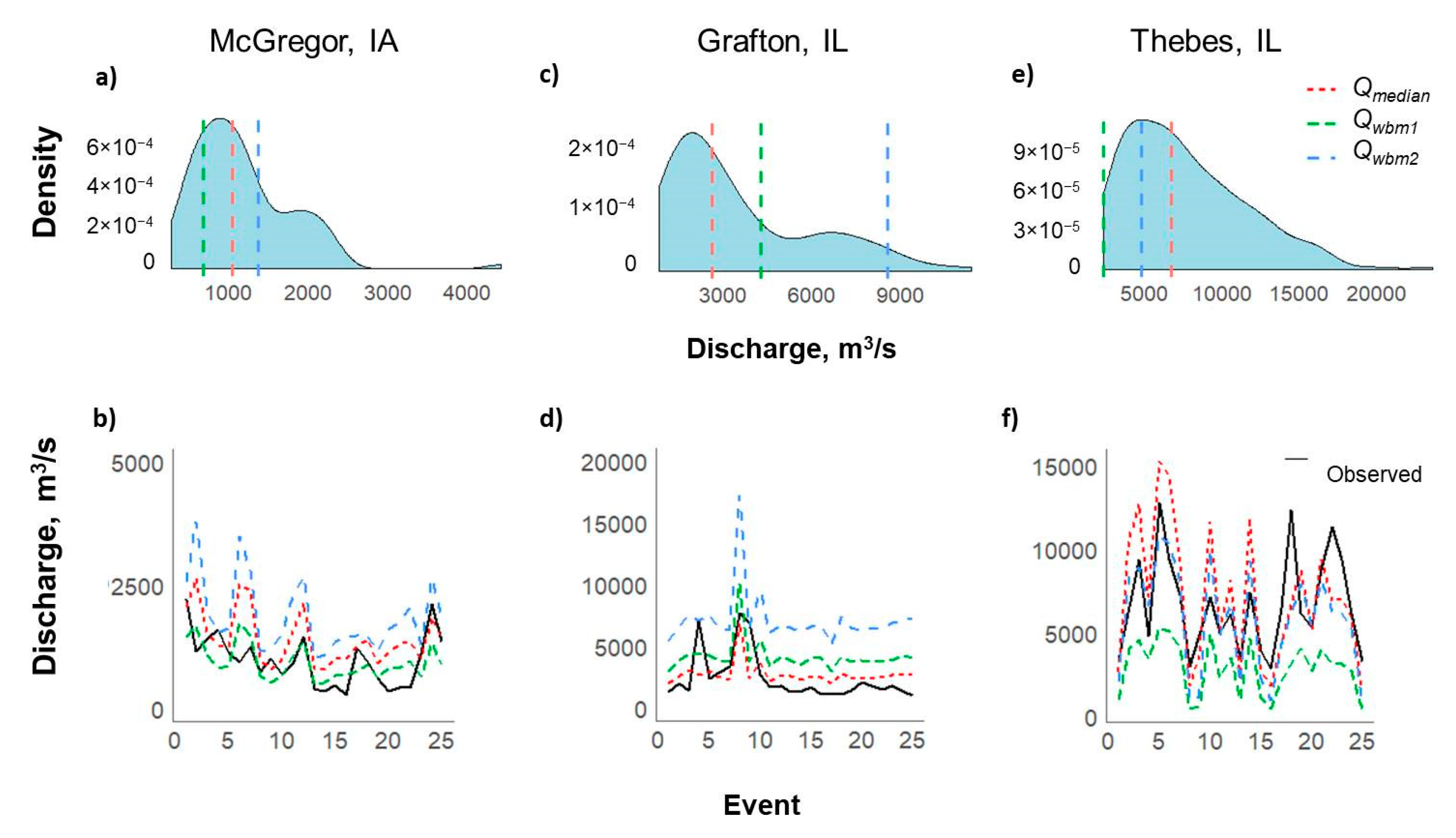
The dependence and sensitivity of the discharge estimates were demonstrated relative to the center of Q prior distribution. Overlaying the three centers of distribution on in situ discharge record density plots revealed which best estimated the peak of the density plot for three representative study sites (Figure 7). Q_wbm1 is most adjacent to the peak of the discharge density plot for the study site at McGregor, IA (Figure 7a). As expected, using this center for Q prior yielded a better discharge estimate than using either of the other two centers of distribution (Figure 7b). Similarly, Q_median appears most adjacent to the peak of the in situ discharge density plot for the study site at Grafton, IL (Figure 7c), so using Q_median as the center of distribution for Q prior led to better performance in estimating the discharge than using either Q_wbm1 or Q_wbm2 (Figure 7d). For the study site at Thebes, IL (Figure 7e,f), the use of Q_wbm2 as the center for the Q prior distribution produced the best discharge estimate because this center is the most adjacent to the peak of the discharge density plot for this river segment. Using an underestimated center for the Q prior distribution tends to underestimate the discharge, and using an overestimated center for the Q prior will likely overestimate the discharge.

3.2.2. Width-Based Discharge Estimates

The performance of Bayesian-AMHG inference using the river widths obtained from the 779 Landsat images (filtered and post-processed) and three different Q prior centers is summarized in

Table 4. Performance of the three Q prior centers (Q_median, Q_wbm1, and Q_wbm2) for estimating river discharge.

Site	Location	Observed Range (m3/s)	N	Relative Bias			MAE (m3/s)			RRMSE			NSE
				Qmedian	Qwbm1	Qwbm2	Qmedian	Qwbm1	Qwbm2	Qmedian	Qwbm1	Qwbm2	Qmedian	Qwbm1	Qwbm2
1	Brooklyn Park, MN	60–968	34	0.07	−0.14	0.71	145	139	282	0.60	0.57	1.10	0.25	0.35	−0.46
2	Winona, MN	187–2720	24	−0.09	−0.22	0.54	389	393	650	0.68	0.75	0.98	0.25	0.16	−0.08
3	McGregor, IA	295–4420	99	0.21	−0.2	0.52	527	426	794	0.54	0.52	0.80	0.11	0.19	−0.29
4	Clinton, IA	547–3630	37	0.13	−0.11	0.38	550	503	848	0.32	0.32	0.53	0.45	0.40	0.10
5	Grafton, IL	813–11400	107	−0.19	0.23	1.09	1850	2260	4070	0.73	0.8	1.44	−0.02	−0.21	−0.88
6	Alton, IL	1010–8160	22	−0.06	−0.19	0.49	1430	1630	2150	0.45	0.49	0.69	0.30	0.29	0.16
7	St. Louis, MO	1940–22800	121	0.13	−0.68	−0.35	1470	4370	2320	0.47	0.82	0.45	0.58	0.56	0.84
8	Chester, IL	1870–16500	166	0.16	−0.66	−0.19	1760	4120	1410	0.37	0.79	0.37	0.59	0.36	0.63
9	Thebes, IL	2720–23600	169	−0.05	−0.59	−0.18	1540	4520	1800	0.28	0.68	0.32	0.70	0.55	0.72
Average across study sites				±0.12	±0.34	±0.49	1074	2040	1590	0.49	0.64	0.74	0.36	0.29	0.08

. Results varied across the nine study sites. As expected, the relative bias was found to be lower with the aid of USGS gauge records (for Q_median) than the approximated mean discharge obtained from either empirical water balance model. An average relative bias of ±0.12 was obtained for all the study sites and found within the “satisfactory” (±0.25) category [63]. Large errors were observed with the use of Q_wbm1 and Q_wbm2 with frequent underestimation (negative bias) and overestimation (positive bias). These results are similar in terms of RRMSE. A lower RRMSE with an average of 0.49 was obtained using Q_median, whereas the estimations with empirically approximated Q priors resulted in a higher average RRMSE (>0.60). Further, the highest NSE was also obtained with Q_median, averaging 0.36 for all the study sites. Among all sites, study site 5 at Grafton, IL, produced the highest MAE (>1850 m³/s) and RRMSE (>0.70) with negative NSEs regardless of which Q prior was used. Even with a rather large number of images (N = 107), this site posed a challenge for river width inference, possibly due to the large width (947.6 m) and standard deviation (98.9 m) (Table 3). In relative terms, study sites 7, 8, and 9, the three farthest downstream sites, were the best sites for predicting discharge using either Q_median or Q_wbm2 as prior information. Despite the unexpected result that Q_wbm2 improved the discharge estimates for these three sites, the estimates themselves were poor for the remaining sites, as indicated by a higher positive bias and RRMSE averaging 0.62 and 0.92, respectively.

Discharge estimates were generally improved by using Q_median in the priors (Figure 8). The Bayesian-AMHG estimates and the in situ discharge records are agreeable (NSE ≥ 0.25) for all the study sites except McGregor, IA, and Grafton, IL. Further, the performance of the Bayesian-AMHG was the best for the three farthest downstream sites, which generally matched the measured discharge with an average relative bias of 0.08, MAE of 1591 m³/s, RRMSE of 0.37, and NSE of 0.62.

3.3. Suspended Sediment Concentration Estimation

3.3.1. Gauge-Specific SSC-SR Model

The regression models for SSC vs. SR are significant at a significance level of 0.05 for all study sites (

Table 5. Gauge-specific functions developed for SSC estimation.

Site	Location	SSC Range (mg/L)	N	Function *	p-Value	R2
1	Brooklyn Park, MN	2–46	38	y = 0.05x + 0.78	0.004	0.21
2	Winona, MN	3–56	37	y = 0.06x + 0.72	0.006	0.20
3	McGregor, IA	3.2–190	86	y = 0.07x + 0.71	<0.001	0.26
4	Clinton, IA	2–127	12	y = 0.03x + 0.84	0.017	0.45
5	Grafton, IL	12.2–796	349	y = 0.13x + 0.37	<0.001	0.40
6	Alton, IL	12.4–324	54	y = 0.06x + 0.64	<0.001	0.27
7	St. Louis, MO	27.4–2340	747	y = 0.13x + 0.36	<0.001	0.66
8	Chester, IL	35–1280	226	y = 0.15x + 0.28	<0.001	0.64
9	Thebes, IL	23.6–961	305	y = 0.13x + 0.36	< 0.001	0.54

* y = red to green band reflectance ratio, x = ln (SSC).

). SSC tends to increase as the water-leaving reflectance from the red band exceeds that from the green band. The functions are similar for study sites 1, 2, 3, 4, and 6 with an average R² of 0.28. Meanwhile, study sites 5, 7, 8, and 9 have similar regression coefficients, with higher slopes and an average R² of 0.61. Of the nine sites, the three farthest downstream have the greatest R² for the SSC-SR regressions: 0.66 for St. Louis, MO; 0.64 for Chester, IL; and 0.54 for Thebes, IL.

3.3.2. Regional-Scale SSC-SR Model

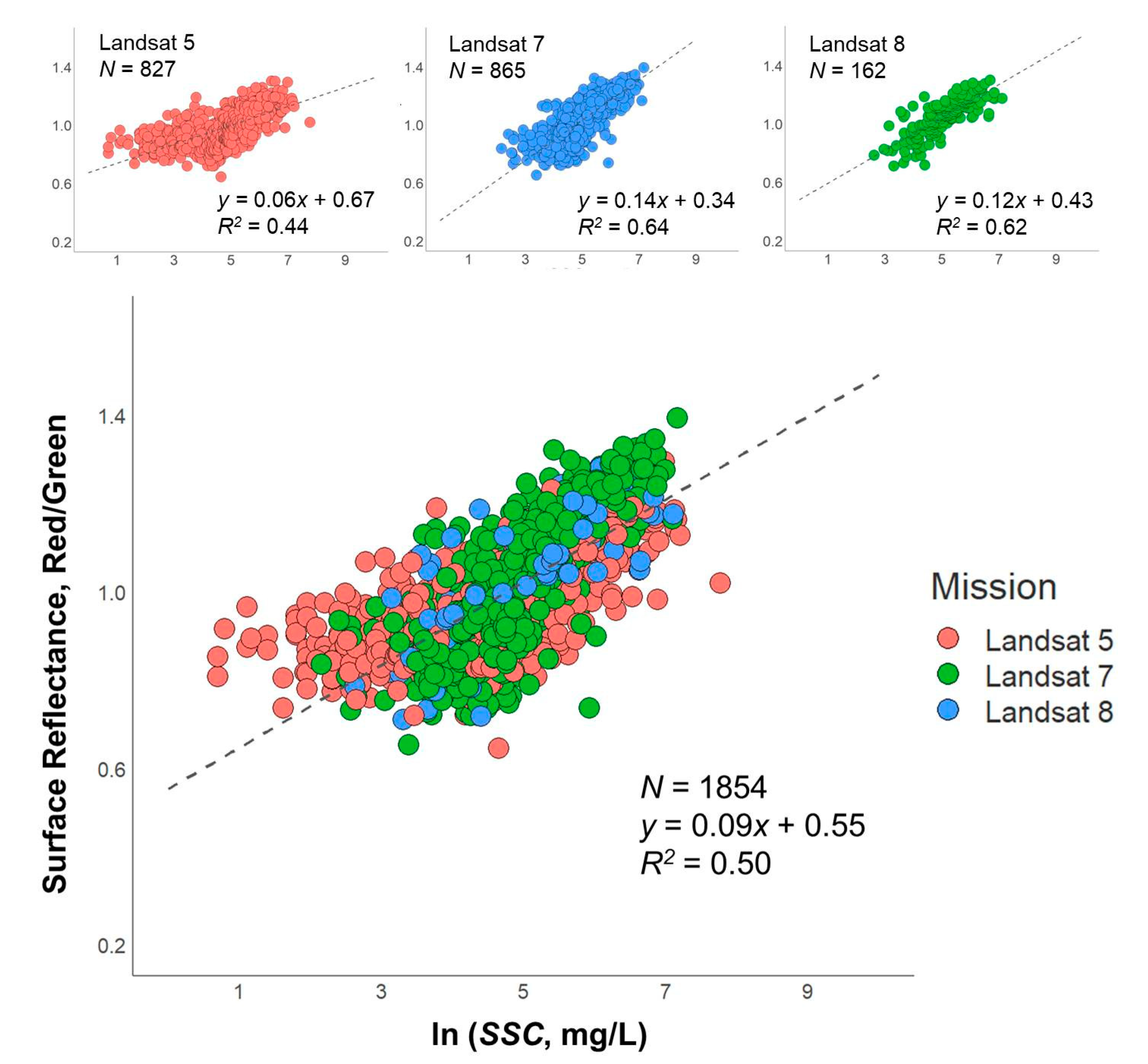
The regional SSC-SR model is significant at a significance level of 0.05 for all missions: Landsat 5 (p-value < 0.001, R² = 0.44), Landsat 7 (p-value < 0.001, R² = 0.64), and Landsat 8 (p-value < 0.001, R² = 0.62). Landsats 7 and 8 exhibit similar patterns of clustering, while as previously discussed, the dispersion in the low SSC range in the Landsat 5 regression is due to the upstream Landsat 5-dominated sites. The regression model for the region with data from all three missions used was also significant at the 0.05 level (p-value < 0.001, R² = 0.50) and “acceptable” (Figure 9) [63].

The estimation of SSC with the regional model results in a high positive bias, RRMSE, and mostly negative NSEs for most of the gauging sites (

Table 6. Performance of gauge-specific and regional SSC-SR models.

Site	Location	Observed Range (mg/L)	N	Relative Bias		MAE (mg/L)		RRMSE		NSE
				Gauge-Specific	Regional	Gauge-Specific	Regional	Gauge-Specific	Regional	Gauge-Specific	Regional
1	Brooklyn Park, MN	5.6–100	29	0.78	0.22	30.8	45.6	2.52	2.68	−6.71	−4.34
2	Winona, MN	6.0–26	22	0.19	1.32	13.7	22.0	1.46	2.35	−9.36	−17.7
3	McGregor, IA	4.0–361	93	0.28	1.09	31.4	42.5	1.85	2.17	−1.33	−1.43
4	Clinton, IA	2.0–198	20	1.23	0.58	109	50.7	2.31	1.06	−5.56	−0.34
5	Grafton, IL	19.9–487	105	0.35	0.95	95.3	183	1.30	3.06	−2.18	−16.1
6	Alton, IL	19.8–373	11	1.40	−0.13	241	77.9	2.66	0.84	−6.11	0.06
7	St. Louis, MO	34.0–1250	115	0.09	0.30	98.4	153	0.59	1.06	0.50	−0.56
8	Chester, IL	39.0–863	79	0.25	1.04	122	324	0.68	2.14	0.16	−6.31
9	Thebes, IL	44.3–1110	147	0.22	0.86	129	294	0.73	1.95	−0.07	−5.83
Average across Study Sites				±0.53	±0.72	96.6	132	1.57	1.92	−3.41	−5.84

). The only positive NSE was obtained for the study site at Alton, IL, with a relative bias of −0.13 and MAE of 77.9 mg/L. In comparison to the regional model, most gauge-specific models yielded a lower RRMSE and higher NSE. Interestingly, the SSC estimates for the three farthest downstream sites at St. Louis, MO; Chester, IL; and Thebes, IL, using their respective gauge-specific models, were all reasonable, with an SSC ranging from 2–1250 mg/L and NSE averaging 0.20. These results were supported by other statistical metric averages: a relative bias of 0.19, MAE of 116.3 mg/L, and RRMSE of 0.67.

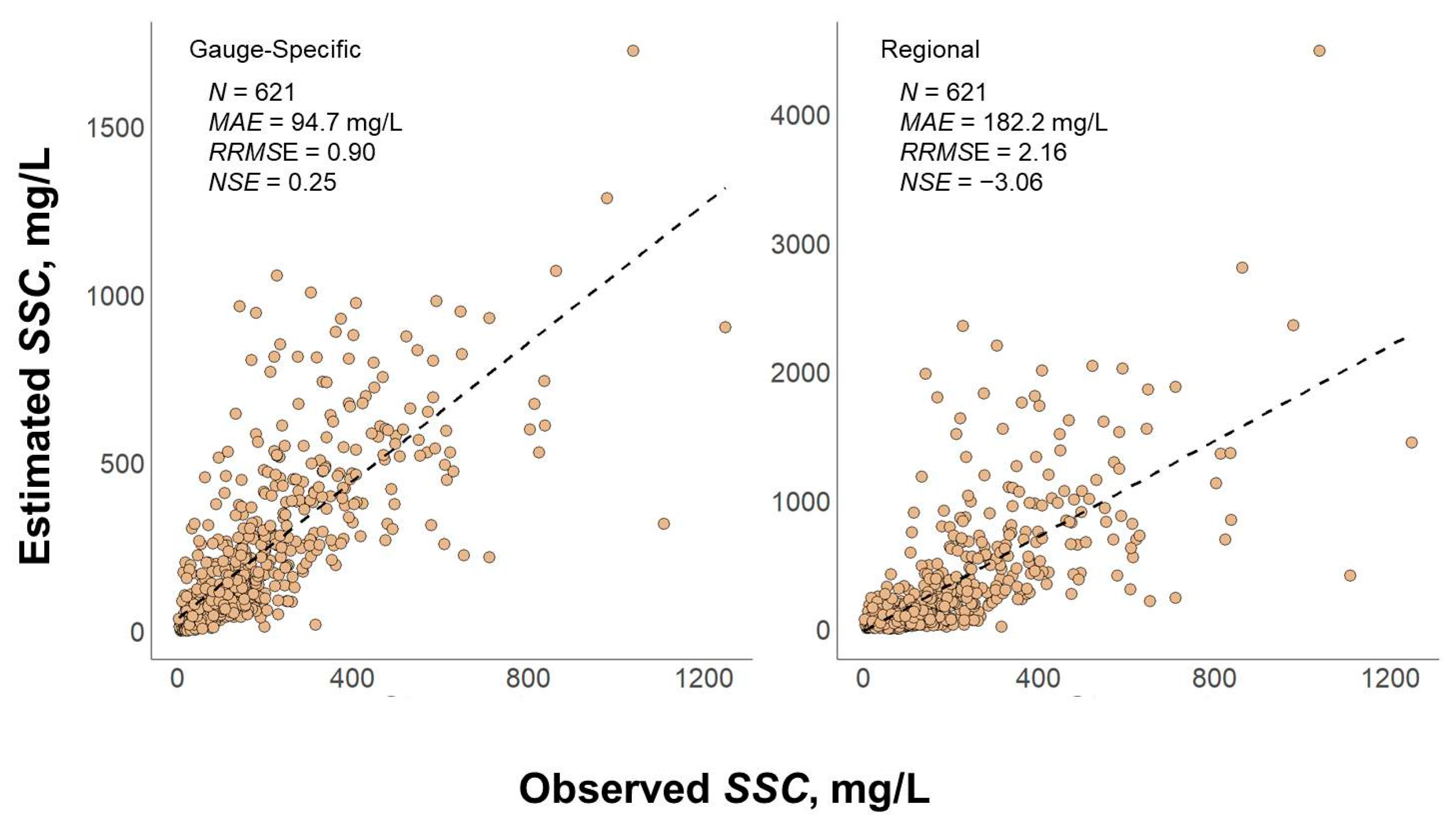
Clearly, using gauge-specific models is better than using a regional model in estimating the SSC for the study sites. The regional model led to an overall MAE of 182.2 mg/L, RRMSE of 2.16, and a negative NSE of −3.06 (Figure 10). In contrast, the gauge-specific SSC-SR models yielded better estimations, with a lower MAE of 94.7 mg/L, RRMSE of 0.90, and a positive NSE of 0.25.

3.4. Sediment Discharge Estimation

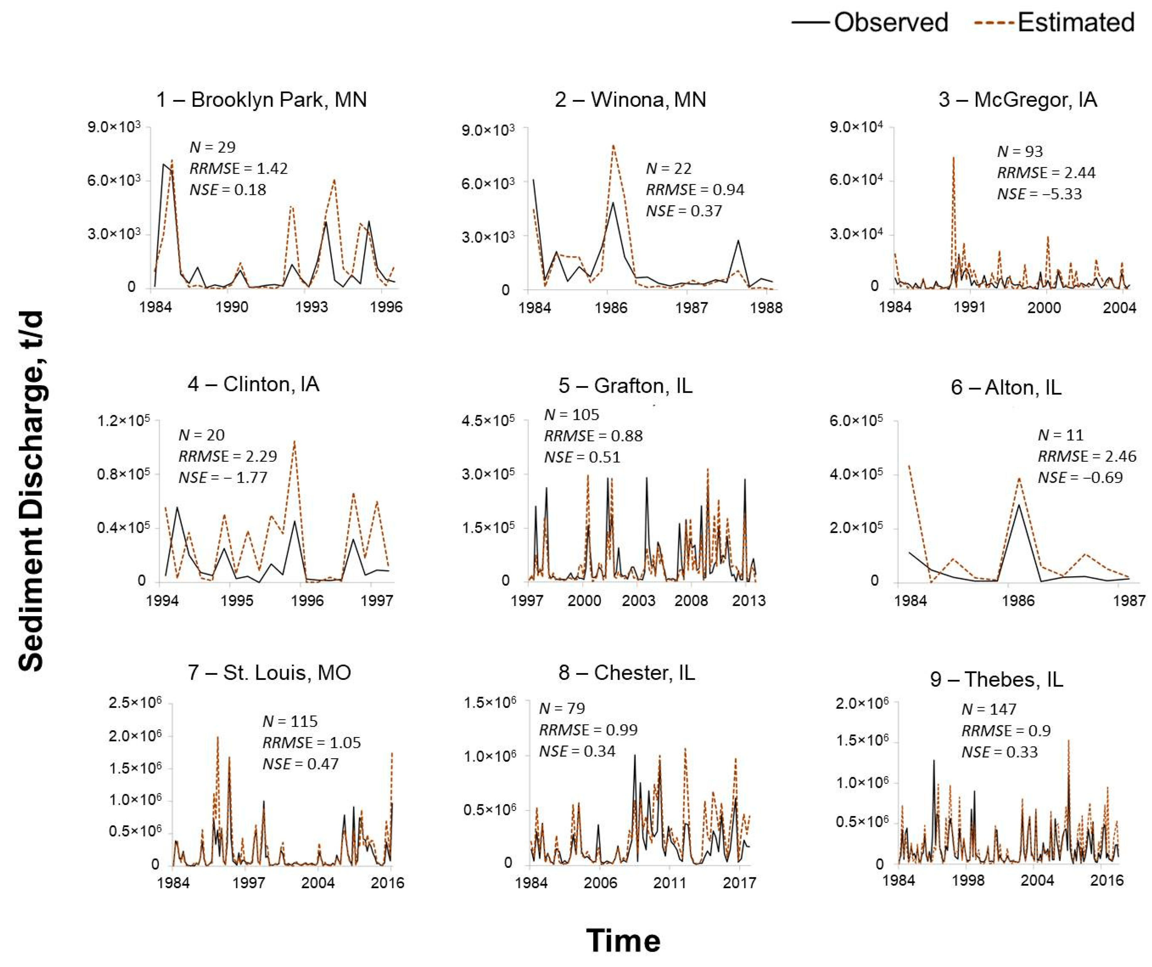
By combining the discharge estimates with the SSC estimates from the gauge-specific model, we calculated sediment discharge for the nine study sites for 621 Landsat images (Figure 11). Interestingly, the site with the best sediment discharge estimates, in terms of RRMSE (0.88) and NSE (0.51), is 5, Grafton, IL. Estimated and observed sediment discharges are generally agreeable among the nine sites, following a similar trend over time. However, extreme events were noticeably overestimated for some images, especially for McGregor, IA; Clinton, IA; and Alton, IL. The second-best study site is 7, St. Louis, MO, with an RRMSE of 1.05 and NSE of 0.47. The estimation appeared problematic at study site 3, McGregor, IA, with a high RRMSE (2.44) and a negative NSE (−5.33).

Combining the discharge and SSC retrieval from Landsat imagery for certain river segments can produce reasonable sediment discharge estimates, as confirmed by comparison with in situ field measurements ranging from 1.78 × 10² to 1.64 × 10⁶ t/d. The relative biases and errors were reduced by using the discharge estimates for gauged settings and a gauge-specific SSC retrieval model. We obtained an average relative bias of 0.23, RRMSE of 0.95, and NSE of 0.40 in simulating the sediment discharge at the USGS gauging sites at Winona, MN; Grafton, IL; St. Louis, MO; Chester, IL; and Thebes, IL (

Table 7. Model performance of sediment discharge estimation for the individual study sites.

Site	Location	Observed Range (t/d)	N	Relative Bias	MAE (t/d)	RRMSE	NSE
1	Brooklyn Park, MN	7.7 × 101–6.95 × 103	29	1.38	8.78 × 102	1.42	0.18
2	Winona, MN	1.78 × 102–6.11 × 103	22	0.03	7.64 × 102	0.94	0.37
3	McGregor, IA	1.46 × 102–1.96 × 104	93	0.63	3.48 × 103	2.44	−5.33
4	Clinton, IA	2.41 × 102–5.58 × 104	20	1.18	2.17 × 104	2.29	−1.77
5	Grafton, IL	2.09 × 102–2.64 × 105	105	−0.09	2.62 × 104	0.88	0.51
6	Alton, IL	5.44 × 103–2.63 × 105	11	1.38	7.18 × 104	2.46	−0.69
7	St. Louis, MO	8.56 × 103–1.64 × 106	115	0.25	8.88 × 104	1.05	0.47
8	Chester, IL	7.52 × 103–1.01 × 106	79	0.40	1.16 × 105	0.99	0.34
9	Thebes, IL	1.38 × 103–1.29 × 106	147	0.22	1.02 × 105	0.90	0.33

). On the other hand, the estimations for the remaining sites were problematic with a higher relative bias (>0.60) and lower NSE (<0.20).

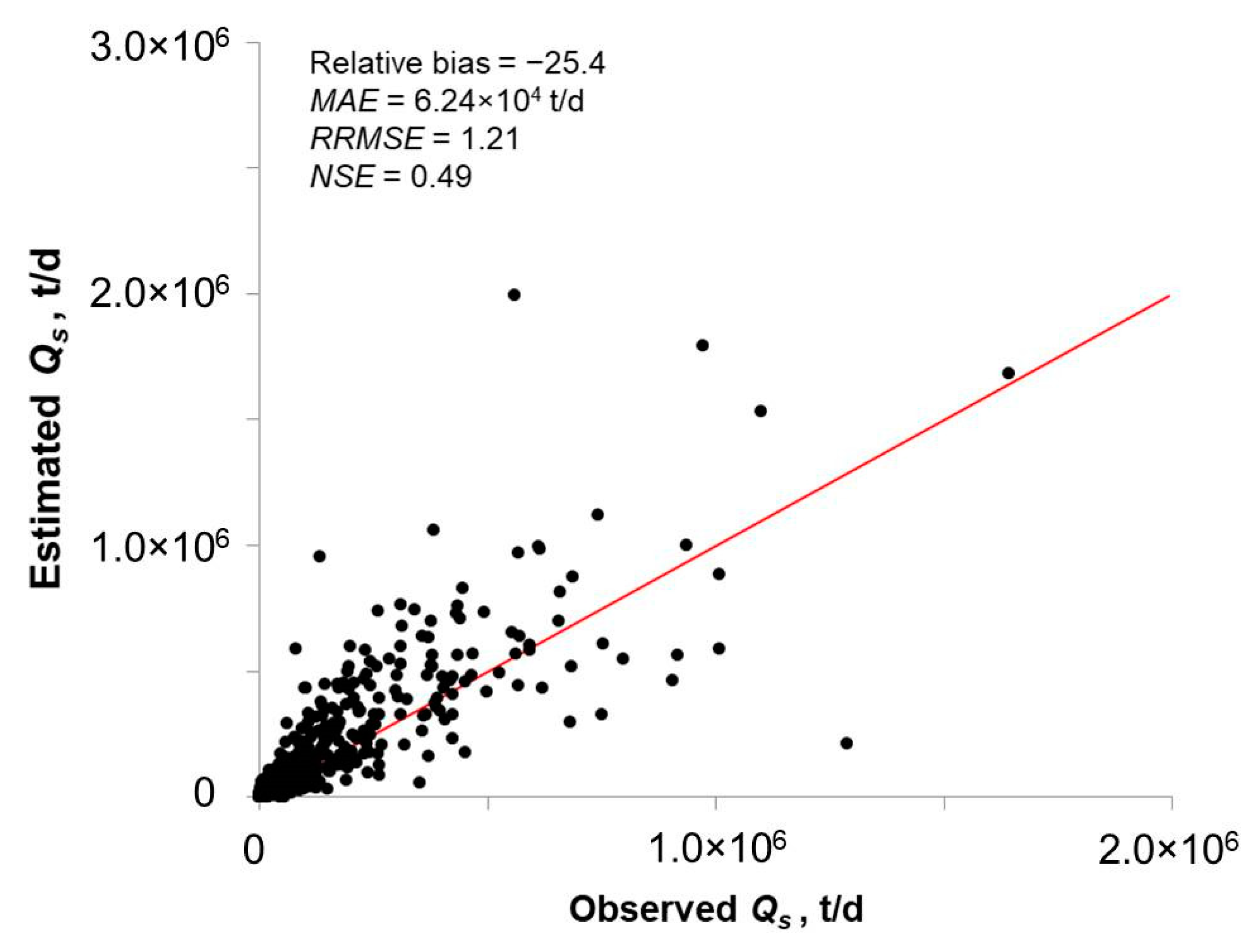
The overall performance of the sediment discharge estimation is illustrated in Figure 12. With 621 Landsat scenes available across all study sites, we obtained a relative bias of −25.4, MAE of 6.24 × 10⁴ t/d, RRMSE of 1.21, and NSE of 0.49. Moriasi et al. [63] recommended that model performance for sediment simulation have a relative bias ± 0.55 and NSE > 0.50 in order to be classified as satisfactory. Their model performance rating is aimed at monthly time step hydrologic simulations for a drainage basin, whereas the method described here is for independent events, at time intervals given by available Landsat imagery for the river reach.

4. Discussion

Our results of estimating river discharge using Landsat imagery support the finding of Feng et al. [38] that the use of Bayesian-AMHG provides better discharge estimates for gauged rivers than for an ungauged setting for which Q priors are approximated from data reanalysis. We also observed that the closer the center of distribution for Q prior was to the peak of the discharge density plot, the more likely the discharge estimate would agree with the observed value. Hence, future studies should further explore how to best approximate the center of distribution of river discharge solely from remotely sensed data.

Our results also suggest that outputs from RivWidthCloud can be effectively used for Bayesian-AMHG discharge inference. The consistency of this automated width retrieval provides a substantial advantage over manual delineation of river widths from remotely sensed imagery. The sediment discharge estimates for the three study sites farthest downstream were “satisfactory” (±0.25 relative bias and NSE > 0.50) following the model performance evaluation criteria recommended by Moriasi et al. [63]. We posit that these results are associated with the morphologic difference between reaches of the study sites. The Rosgen Type I plan view classification of natural rivers broadly characterizes channels as relatively straight (class A), low sinuosity (class B), meandering (class C), braided (class D), anastomosed (class DA), and tortuously meandering (class E) [64]. Study sites 1–6 possess class D channel type features (see Figure 4): complex multiple or braided channels with wide eroding banks. In contrast, study sites 7, 8, and 9 have entrenched and stable channels, more characteristic of class A or B. Consequently, we consider that the selection of a representative reach for a river system is crucial for multi-river studies because the performance in estimating discharge from optical sensors varies widely from one reach to another.

We also observed different patterns in our developed SSC-SR retrieval models. Study sites 1, 2, 3, 4, and 6, which have nearly identical regression functions (Table 5), were likely influenced by the low SSC levels (2–324 mg/L) and by Landsat 5 being the predominant sensor platform used to acquire their images. The lower SSC levels at these study sites may have led to a weaker correlation with the water-leaving reflectance captured in the Landsat 5 images. Further, most of these sites have a higher mean green band than red band reflectance (Figure 6), suggesting that the river segments with low SSC levels or turbidity do not fully illuminate the brownish sediment color in Landsat imagery. This is further confirmed with the regional SSC-SR retrieval model, which shows clearly that Landsat 5 data points differ from Landsats 7 and 8 data points, while the latter two closely match each other (Figure 9). The matching functions for study sites 5, 7, 8, and 9 may be a result of the dominance of the Landsat sensor used and to the proximity of the study sites. In most cases, these study sites were in the same Landsat image, as they share adjacent or similar Landsat acquisition paths/rows (path 24, row 33 and path 23, row 34; Table 2). It is worth noting that SSCs at these sites are higher (12.2–2340 mg/L) than the other five sites, suggesting that sites with lower SSC levels and captured by Landsat 5 likely have a lower coefficient of determination for the SSC-SR model.

Most published SSC–SR models were based on data from a single Landsat mission (e.g., Landsat 8). Pham et al. [51] presented SSC-SR models (R² = 0.75) using the red to green band ratio from Landsat 8, with 40 images and SSC levels ranging from 22.4–178 mg/L. A related study by Pereira et al. [49] using the red to green band reflectance ratio of 26 Landsat 8 images yielded an SSC-SR model with a similarly high coefficient of determination (R² = 0.86) for SSC levels of 49–533 mg/L. Despite these models being developed with a smaller sample and a lower SSC range in their respective river systems, our results show that the red to green band reflectance ratio from multiple Landsat missions can be used to estimate SSCs of certain reaches in the Upper Mississippi River. This result is consistent with the findings of Markert et al. [48] and Peterson et al. [50], both of which reported SSC-SR models with R² ≈ 0.5 using SR data from multiple Landsat missions (5, 7, and 8). Nonetheless, some biases and errors in our SSC estimates were related to the low sediments in the water column captured by the Landsat 5 sensor. As such, other band combinations should be explored when using Landsat 5 surface reflectance data. Note that the errors may also be due to other variables, such as higher blue and red absorption with the presence of chlorophyll and algae during low flows, and the presence of organic materials upstream in the Upper Mississippi River [59,65].

Studies estimating annual sediment discharge using gauge records and composited remotely sensed data (250-m MODIS) have shown good agreement with observed data with a ±2% mean relative difference [17,42]. Compared with these studies, we demonstrated a “per event” or “per image” estimation approach where we approximated the sediment discharge based on gauge records and 30-m Landsat data. Extreme events, such as the “Great Flood of 1993,” a 100-year flood event, were also covered in our simulations for the nine gauge sites of the Upper Mississippi River. Given that the approach is highly dependent on the accuracy of the discharge and SSC estimates, the uncertainties in their estimates can either increase the magnitude of errors or improve the final sediment discharge estimates, as illustrated in Figure 13. For instance, study site 5 (Grafton, IL), shows a negative relative bias (−0.19) in Q estimates and a positive relative bias (0.35) in SSC estimates. As a result, the Q and SSC errors offset each other to yield an unexpectedly good match between sediment discharge estimates and measurements. Unlike study site 5, site 7 (St. Louis, IL) has a minimal relative bias (<0.15) in both Q and SSC estimates. Thus, we can reasonably expect that this site will have good overall sediment discharge estimates with a low relative bias and better model fit. For this reason, we regard the St. Louis site as the best site within the Upper Mississippi River for estimating sediment discharge using Landsat data.

Future efforts should be devoted to improving the Q and SSC estimation to further advance the utility of Landsat data or other optical remote sensing platforms for sediment discharge estimation in river systems. A river’s Q can be estimated based on channel width, but prior discharge information is required to perform the Bayesian-AMHG inference. Readily accessible prior mean discharge of river reaches, e.g., from Lin et al. [66], may be examined to apply discharge estimations to ungauged rivers. Alternative approaches to estimating SSC, such as non-linear regression and machine learning estimation [50], should be explored. Last, even without gauge records for calibrations, a method estimating water and sediment discharge in rivers using remotely sensed data would still be useful in evaluating and screening for those susceptible to extreme flooding events or exhibiting excessive sedimentation.

5. Conclusions

We explored the potential of using remotely sensed images to estimate the discharge of water and sediment in a river system. In many cases, traditional monitoring operations are hampered by accuracy requirements, cost, and safety concerns regarding their labor-intensive field sampling methods. For this reason, the number of active gauging stations in many areas across the US continues to decline, despite increasing demands to monitor flow, sediment transport, and other aspects of river health. Our alternative approach, using space-based observations to assess the status of river systems, helps to address this need.

Conclusions from this study are:

• Width outputs from RivWidthCloud can be effectively used for Bayesian-AMHG inference of river discharge.
• Discharge estimations are influenced by both prior information and morphologic features along the river.
• Higher biases and errors in SSC estimates tended to result from Landsat 5 sensors capturing scenes with low sediment levels in the water column. This suggests that for Landsat 5 surface reflectance data, additional band combinations should be explored.
• Landsat imagery-based estimates of Q and SSC can yield reasonable sediment discharge estimates. In this study of the Upper Mississippi River, estimates had a relative bias of −25.4, MAE of 6.24 × 10⁴ t/d, RRMSE of 1.21, and NSE of 0.49.
• Because sediment discharge estimates are the product of two other independent estimates (water discharge and SSC), biases and errors from these component estimates can either increase or decrease the magnitude of errors in the sediment discharge estimates.
• Even without gauge records for calibrations, this method can be used to estimate water and sediment discharges of rivers, and to evaluate and screen for rivers susceptible to extreme flooding or exhibiting excessive sedimentation.

This study demonstrates the potential of estimating water and sediment discharges—crucial hydrological information—using remotely sensed data as an alternative to labor-intensive field methods. Future efforts should be devoted to refining the Q and SSC estimation to further advance the utility of Landsat data for sediment discharge estimation in river systems.

References

- Aylward, B.; Bandyopadhyay, J.; Belausteguigotia, J.C. Freshwater ecosystem services. In Ecosystems and Human Well-Being: Policy Responses; Island Press: Washington, DC, USA, 2005; Volume 3, pp. 213–254. [Google Scholar]
- Böck, K.; Polt, R.; Schülting, L. Ecosystem services in river landscapes. In Riverine Ecosystem Management; Springer: Cham, Switzerland, 2018; pp. 413–433. [Google Scholar]
- Khatri, N.; Tyagi, S. Influences of natural and anthropogenic factors on surface and groundwater quality in rural and urban areas. Front. Life Sci. 2015, 8, 23–39. [Google Scholar] [CrossRef]
- Adeosun, F.; Adams, T.; Amrevuawho, M. Effect of anthropogenic activities on the water quality parameters of federal university of agriculture Abeokuta reservoir. Int. J. Fish. Aquat. Stud. 2016, 4, 104–108. [Google Scholar]
- Cheng, Y.; He, H.; Cheng, N.; He, W. The effects of climate and anthropogenic activity on hydrologic features in Yanhe River. Adv. Meteorol. 2016, 2016, 1–11. [Google Scholar] [CrossRef] [Green Version]
- Zhang, X.F.; Yan, H.C.; Yue, Y.; Xu, Q.X. Quantifying natural and anthropogenic impacts on runoff and sediment load: An investigation on the middle and lower reaches of the Jinsha River Basin. J. Hydrol. Reg. Stud. 2019, 25, 100617. [Google Scholar] [CrossRef]
- Chimwanza, B.; Mumba, P.P.; Moyo, B.H.Z.; Kadewa, W. The impact of farming on river banks on water quality of the rivers. Int. J. Environ. Sci. Technol. 2006, 2, 353–358. [Google Scholar] [CrossRef] [Green Version]
- Ayobahan, S.U.; Ezenwa, I.M.; Orogun, E.E.; Uriri, J.E.; Wemimo, I.J. Assessment of anthropogenic activities on water quality of Benin River. J. Appl. Sci. Environ. Manag. 2014, 18, 629–636. [Google Scholar] [CrossRef] [Green Version]
- Gunawardena, A.; Wijeratne, E.M.S.; White, B.; Hailu, A.; Pandit, R. Industrial pollution and the management of river water quality: A model of Kelani River, Sri Lanka. Environ. Monit. Assess. 2017, 189, 457. [Google Scholar] [CrossRef]
- Camara, M.; Jamil, N.R.; Abdullah, A.F.B. Impact of land uses on water quality in Malaysia: A review. Ecol. Process. 2019, 8, 10. [Google Scholar] [CrossRef]
- Chetty, S.; Pillay, L. Assessing the influence of human activities on river health: A case for two South African rivers with differing pollutant sources. Environ. Monit. Assess. 2019, 191, 168. [Google Scholar] [CrossRef]
- Gordon, C.; Nukpezah, D.; Lawson, E.T.; Ofori, B.D.; Tawiah, D.Y.; Pabi, O.; Ayivor, J.S.; Koranteng, D.; Mensah, A.M. West Africa—Water resources vulnerability using a multidimensional approach: Case study of Volta Basin. Clim. Vulnerability 2013, 2, 283–309. [Google Scholar]
- Hauer, C.; Leitner, P.; Unfer, G.; Pulg, U.; Habersack, H.; Graf, W. The role of sediment and sediment dynamics in the aquatic environment. In Riverine Ecosystem Management; Springer: Cham, Switzerland, 2018; pp. 151–169. [Google Scholar]
- Tundu, C.; Tumbare, M.J.; Onema, J.M.K. Sedimentation and its impacts/effects on river system and reservoir water quality: Case study of Mazowe catchment, Zimbabwe. Proc. Int. Assoc. Hydrol. Sci. 2018, 377, 57. [Google Scholar] [CrossRef] [Green Version]
- Walling, D.E. The United Nations world water assessment programme. In The Impact of Global Change on Erosion and Sediment Transport by Rivers: Current Progress and Challenges; UNESCO: Paris, France, 2009. [Google Scholar]
- Walling, D.E.; Fang, D. Recent trends in the suspended sediment loads of the world’s rivers. Glob. Planet. Chang. 2003, 39, 111–126. [Google Scholar] [CrossRef]
- Martinez, J.M.; Guyot, J.L.; Filizola, N.; Sondag, F. Increase in suspended sediment discharge of the Amazon River assessed by monitoring network and satellite data. Catena 2009, 79, 257–264. [Google Scholar] [CrossRef] [Green Version]
- Wang, S.; Fu, B.; Piao, S.; Lü, Y.; Ciais, P.; Feng, X.; Wang, Y. Reduced sediment transport in the Yellow River due to anthropogenic changes. Nat. Geosci. 2016, 9, 38–41. [Google Scholar] [CrossRef]
- Engstrom, D.R.; Almendinger, J.E.; Wolin, J.A. Historical changes in sediment and phosphorus loading to the upper Mississippi River: Mass-Balance reconstructions from the sediments of Lake Pepin. J. Paleolimnol. 2009, 41, 563–588. [Google Scholar] [CrossRef]
- Holeman, J.N. The sediment yield of major rivers of the world. Water Resour. Res. 1968, 4, 737–747. [Google Scholar] [CrossRef]
- Milliman, J.D.; Meade, R.H. World-Wide delivery of river sediment to the oceans. J. Geol. 1983, 91, 1–21. [Google Scholar] [CrossRef]
- Meade, R.H.; Moody, J.A. Causes for the decline of suspended-sediment discharge in the Mississippi River system, 1940–2007. Hydrol. Process. Int. J. 2010, 24, 35–49. [Google Scholar] [CrossRef]
- Porterfield, G. Computation of fluvial-sediment discharge. In US Geological Survey Techniques of Water-Resources Investigations; US Government Printing Office: Washington, DC, USA, 1972. [Google Scholar]
- Gray, J.R.; Simões, F.J. Estimating sediment discharge. In Sedimentation Engineering—Processes, Measurements, Modeling, and Practice Manual; American Society of Civil Engineers (ASCE): Reston, VA, USA, 2008; Volume 110, pp. 1067–1088. [Google Scholar]
- Borah, D.K. Sediment discharge model for small watersheds. Trans. ASAE 1989, 32, 0874–0880. [Google Scholar] [CrossRef]
- Wang, G.; Hapuarachchi, P.; Ishidaira, H.; Kiem, A.S.; Takeuchi, K. Estimation of soil erosion and sediment yield during individual rainstorms at catchment scale. Water Resour. Manag. 2009, 23, 1447–1465. [Google Scholar] [CrossRef]
- Prosser, I.P.; Rutherfurd, I.D.; Olley, J.M.; Young, W.J.; Wallbrink, P.J.; Moran, C.J. Corrigendum to: Large-Scale patterns of erosion and sediment transport in river networks, with examples from Australia. Mar. Freshw. Res. 2001, 52, 817. [Google Scholar] [CrossRef]
- Merritt, W.S.; Letcher, R.A.; Jakeman, A.J. A review of erosion and sediment transport models. Environ. Model. Softw. 2003, 18, 761–799. [Google Scholar] [CrossRef]
- Smith, L.C. Satellite remote sensing of river inundation area, stage, and discharge: A review. Hydrol. Process. 1997, 11, 1427–1439. [Google Scholar] [CrossRef]
- Wass, P.D.; Marks, S.D.; Finch, J.W.; Leeks, G.J.L.; Ingram, J.K. Monitoring and preliminary interpretation of in-river turbidity and remote sensed imagery for suspended sediment transport studies in the Humber catchment. Sci. Total Environ. 1997, 194, 263–283. [Google Scholar] [CrossRef]
- Brakenridge, G.R.; Tracy, B.T.; Knox, J.C. Orbital SAR remote sensing of a river flood wave. Int. J. Remote Sens. 1998, 19, 1439–1445. [Google Scholar] [CrossRef]
- Smith, L.C.; Pavelsky, T.M. Estimation of river discharge, propagation speed, and hydraulic geometry from space: Lena River, Siberia. Water Resour. Res. 2008, 44. [Google Scholar] [CrossRef]
- Kuhn, C.; de Matos Valerio, A.; Ward, N.; Loken, L.; Sawakuchi, H.O.; Kampel, M.; Richey, J.; Stadler, P.; Crawford, J.; Striegl, R.; et al. Performance of Landsat-8 and Sentinel-2 surface reflectance products for river remote sensing retrievals of chlorophyll-a and turbidity. Remote Sens. Environ. 2019, 224, 104–118. [Google Scholar] [CrossRef] [Green Version]
- Shen, X.; Wang, D.; Mao, K.; Anagnostou, E.; Hong, Y. Inundation extent mapping by synthetic aperture radar: A review. Remote Sens. 2019, 11, 879. [Google Scholar] [CrossRef] [Green Version]
- Hou, J.; van Dijk, A.I.; Beck, H.E. Global satellite-based river gauging and the influence of river morphology on its application. Remote Sens. Environ. 2020, 239, 111629. [Google Scholar] [CrossRef]
- Yang, X.; Pavelsky, T.M.; Allen, G.H. The past and future of global river ice. Nature 2020, 577, 69–73. [Google Scholar] [CrossRef]
- Gleason, C.J.; Smith, L.C. Toward global mapping of river discharge using satellite images and at-many-stations hydraulic geometry. Proc. Natl. Acad. Sci. USA 2014, 111, 4788–4791. [Google Scholar] [CrossRef] [PubMed] [Green Version]
- Feng, D.; Gleason, C.J.; Yang, X.; Pavelsky, T.M. Comparing discharge estimates made via the BAM algorithm in high-order Arctic rivers derived solely from optical CubeSat, Landsat, and Sentinel-2 data. Water Resour. Res. 2019, 55, 7753–7771. [Google Scholar] [CrossRef]
- Hagemann, M.W.; Gleason, C.J.; Durand, M.T. BAM: Bayesian AMHG-Manning inference of discharge using remotely sensed stream width, slope, and height. Water Resour. Res. 2017, 53, 9692–9707. [Google Scholar] [CrossRef]
- Stumpf, R.P.; Goldschmidt, P.M. Remote sensing of suspended sediment discharge into the western Gulf of Maine during the April 1987 100-year flood. J. Coast. Res. 1992, 8, 218–225. [Google Scholar]
- Mangiarotti, S.; Martinez, J.M.; Bonnet, M.P.; Buarque, D.C.; Filizola, N.; Mazzega, P. Discharge and suspended sediment flux estimated along the mainstream of the Amazon and the Madeira Rivers (from in situ and MODIS Satellite Data). Int. J. Appl. Earth Obs. Geoinf. 2013, 21, 341–355. [Google Scholar] [CrossRef] [Green Version]
- Gallay, M.; Martinez, J.M.; Mora, A.; Castellano, B.; Yépez, S.; Cochonneau, G.; Alfonso, J.A.; Carrera, J.M.; López, J.L.; Laraque, A. Assessing Orinoco river sediment discharge trend using MODIS satellite images. J. S. Am. Earth Sci. 2019, 91, 320–331. [Google Scholar] [CrossRef]
- Mouyen, M.; Longuevergne, L.; Steer, P.; Crave, A.; Lemoine, J.M.; Save, H.; Robin, C. Assessing modern river sediment discharge to the ocean using satellite gravimetry. Nat. Commun. 2018, 9, 1–9. [Google Scholar] [CrossRef] [PubMed] [Green Version]
- Mertes, L.A.; Smith, M.O.; Adams, J.B. Estimating suspended sediment concentrations in surface waters of the Amazon River wetlands from Landsat images. Remote Sens. Environ. 1993, 43, 281–301. [Google Scholar] [CrossRef]
- Lane, S.N.; Westaway, R.M.; Murray Hicks, D. Estimation of erosion and deposition volumes in a large, gravel-bed, braided river using synoptic remote sensing. Earth Surf. Process. Landf. 2003, 28, 249–271. [Google Scholar] [CrossRef]
- Long, C.M.; Pavelsky, T.M. Remote sensing of suspended sediment concentration and hydrologic connectivity in a complex wetland environment. Remote Sens. Environ. 2013, 129, 197–209. [Google Scholar] [CrossRef] [Green Version]
- Villar, R.E.; Martinez, J.M.; Le Texier, M.; Guyot, J.L.; Fraizy, P.; Meneses, P.R.; de Oliveira, E. A study of sediment transport in the Madeira River, Brazil, using MODIS remote-sensing images. J. S. Am. Earth Sci. 2013, 44, 45–54. [Google Scholar] [CrossRef]
- Markert, K.N.; Schmidt, C.M.; Griffin, R.E.; Flores, A.I.; Poortinga, A.; Saah, D.S.; Muench, R.E.; Clinton, N.E.; Chishtie, F.; Kityuttachai, K.; et al. Historical and operational monitoring of surface sediments in the Lower Mekong basin using Landsat and Google Earth Engine cloud computing. Remote Sens. 2018, 10, 909. [Google Scholar] [CrossRef] [Green Version]
- Pereira, L.S.; Andes, L.C.; Cox, A.L.; Ghulam, A. Measuring suspended-sediment concentration and turbidity in the middle mississippi and lower missouri rivers using landsat data. JAWRA J. Am. Water Resour. Assoc. 2018, 54, 440–450. [Google Scholar] [CrossRef]
- Peterson, K.T.; Sagan, V.; Sidike, P.; Cox, A.L.; Martinez, M. Suspended sediment concentration estimation from Landsat imagery along the Lower Missouri and Middle Mississippi Rivers using an extreme learning machine. Remote Sens. 2018, 10, 1503. [Google Scholar] [CrossRef] [Green Version]
- Pham, Q.V.; Ha, N.T.T.; Pahlevan, N.; Oanh, L.T.; Nguyen, T.B.; Nguyen, N.T. Using Landsat-8 images for quantifying suspended sediment concentration in Red River (Northern Vietnam). Remote Sens. 2018, 10, 1841. [Google Scholar] [CrossRef] [Green Version]
- Yepez, S.; Laraque, A.; Martinez, J.M.; De Sa, J.; Carrera, J.M.; Castellanos, B.; Gallay, M.; Lopez, J.L. Retrieval of suspended sediment concentrations using Landsat-8 OLI satellite images in the Orinoco River (Venezuela). Comptes Rendus Geosci. 2018, 350, 20–30. [Google Scholar] [CrossRef]
- Gray, J.R. The need for surrogate technologies to monitor fluvial-sediment transport. In Proceedings of the Turbidity and Other Sediment Surrogates Workshop; 2002. Available online: https://archive.usgs.gov/archive/sites/water.usgs.gov/osw/techniques/TSS/gray.pdf (accessed on 24 January 2020).
- United States Geological Survey. Ecological Status and Trends of the Upper Mississippi River System 1998. A Report of the Long Term Resource Monitoring Program; US Geological Survey, Upper Midwest Environmental Sciences Center: La Crosse, WI, USA, 1999; pp. 1–236.
- Gorelick, N.; Hancher, M.; Dixon, M.; Ilyushchenko, S.; Thau, D.; Moore, R. Google Earth Engine: Planetary-Scale geospatial analysis for everyone. Remote Sens. Environ. 2017, 202, 18–27. [Google Scholar] [CrossRef]
- Yang, X.; Pavelsky, T.M.; Allen, G.H.; Donchyts, G. RivWidthCloud: An automated Google Earth Engine algorithm for river width extraction from remotely sensed imagery. IEEE Geosci. Remote Sens. Lett. 2019, 17, 217–221. [Google Scholar] [CrossRef]
- Leopold, L.B.; Maddock, T. The hydraulic geometry of stream channels and some physiographic implications. In Geological Survey Professional Paper; US Government Printing Office: Washington, DC, USA, 1953; Volume 252. [Google Scholar]
- Edwards, T.K.; Glysson, G.D. Field methods for measurement of fluvial sediment. In US Geological Survey Techniques of Water-Resources Investigations; US Government Printing Office: Washington, DC, USA, 1999. [Google Scholar]
- Han, L. Spectral reflectance with varying suspended sediment concentrations in clear and algae-laden waters. Photogramm. Eng. Remote Sens. 1997, 63, 701–705. [Google Scholar]
- Ha, N.T.T.; Thao, N.T.P.; Koike, K.; Nhuan, M.T. Selecting the best band ratio to estimate chlorophyll-a concentration in a tropical freshwater lake using sentinel 2a images from a case study of Lake Ba Be (Northern Vietnam). ISPRS Int. J. Geoinf. 2017, 6, 290. [Google Scholar] [CrossRef]
- Son, Y.B.; Min, J.E.; Ryu, J.H. Detecting massive green algae (Ulva prolifera) blooms in the Yellow Sea and East China Sea using geostationary ocean color imager (GOCI) data. Ocean Sci. J. 2012, 47, 359–375. [Google Scholar] [CrossRef]
- Pavelsky, T.M.; Smith, L.C. Remote sensing of suspended sediment concentration, flow velocity, and lake recharge in the Peace-Athabasca Delta, Canada. Water Resour. Res. 2009, 45. [Google Scholar] [CrossRef]
- Moriasi, D.N.; Arnold, J.G.; Van Liew, M.W.; Bingner, R.L.; Harmel, R.D.; Veith, T.L. Model evaluation guidelines for systematic quantification of accuracy in watershed simulations. Trans. ASABE 2007, 50, 885–900. [Google Scholar] [CrossRef]
- Rosgen, D.L. A classification of natural rivers. Catena 1994, 22, 169–199. [Google Scholar] [CrossRef] [Green Version]
- Houser, J.N.; Bierman, D.W.; Burdis, R.M.; Soeken-Gittinger, L.A. Longitudinal trends and discontinuities in nutrients, chlorophyll, and suspended solids in the Upper Mississippi River: Implications for transport, processing, and export by large rivers. Hydrobiologia 2010, 651, 127–144. [Google Scholar] [CrossRef]
- Lin, P.; Pan, M.; Beck, H.E.; Yang, Y.; Yamazaki, D.; Frasson, R.; David, C.H.; Durand MPavelsky, T.M.; Allen, G.H.; Gleason, C.J.; et al. Global reconstruction of naturalized river flows at 2.94 million reaches. Water Resour. Res. 2019, 55, 6499–6516. [Google Scholar] [CrossRef] [Green Version]
Figure 1.
Study sites in the Upper Mississippi River.
Figure 2.
Timeline of Landsat mission operations. Source: https://landsat.gsfc.nasa.gov/.
Figure 3.
An example of filtering of river widths at Alton, IL, using a Landsat 5 image captured on 16 June 1984. (A) Raw width outputs obtained from RivWidthCloud. (B) Filtered widths within a ~1-km distance from a USGS gauge location.
Figure 4.
Sampling areas for Landsat surface reflectance retrieval at the study sites.
Figure 5.
Flowchart of estimating sediment discharge with Landsat imagery.
Figure 6.
Mean surface reflectance at each study site obtained from the three Landsat missions.
Figure 7.
Effect of the centers of distribution for Q prior on discharge estimates with study sites 3, 5, and 9 as examples. Top panel: three different centers of distribution over the density plot of gauge discharge records (a,c,e):. Bottom panel: effect of the centers on the discharge estimates for the first 25 events from available Landsat imagery (b,d,f).
Figure 8.
Estimated and observed river discharges (1984–2017) for the nine study sites in the Upper Mississippi River. The dashed line represents the 1:1 relationship.
Figure 9.
Regional SSC-SR models for the Upper Mississippi River. Top panel: regression models for each Landsat mission. Bottom panel: regional regression model for all the Landsat missions.
Figure 10.
Comparison of gauge-specific (left) and regional (right) SSC-SR models for the Upper Mississippi River. Note the different y-axis scales. The dashed line represents the 1:1 relationship.
Figure 11.
Estimated and observed sediment discharges for the individual study sites.
Figure 12.
Overall performance of the sediment discharge estimation for the nine study sites in the Upper Mississippi River. The red line denotes the 1:1 relationship.
Figure 13.
Effect of relative biases in Q and SSC estimation on sediment discharge estimation for the study sites in the Upper Mississippi River. Left panel: relative bias in sediment discharge estimation. Right panel: relative bias in Q and SSC estimation.