Use of Moon Observations for Characterization of Sentinel-3B Ocean and Land Color Instrument

Abstract

During the commissioning of the Sentinel-3B satellite, a single lunar observation was performed to assess the possible use of the moon for characterization and validation of onboard instruments. The observation was carried out in stable orientation after a roll maneuver, allowing the moon to be imaged by the Earth view of instruments. Data acquired by the Ocean Land Color Instrument (OLCI) allowed inflight verification of stray-light correction (SLC) performed by the Mission Performance Centre (MPC), and assessment of radiometric behavior of instrument in comparison with lunar irradiance models performed in cooperation between European Space Research and Technology Centre (ESTEC) and European Organisation for the Exploitation of Meteorological Satellites (EUMETSAT). This paper describes the results of those activities along with the proposed update of stray-light correction developed with the use of lunar data.

1. Introduction

The Sentinel-3 (S3) mission is a part of the Copernicus Space Component (CSC)—the European Commission’s Earth Observation program. The main objectives of the S3 mission are measurements of sea surface topography, sea and land surface temperature as well as ocean and land color to support forecasting systems and environmental and climate monitoring. S3 payloads include Ocean and Land Colour Instrument (OLCI), Sea and Land Surface Temperature Radiometer (SLSTR), Synthetic Aperture Radar Altimeter (SRAL) and MicroWave Radiometer (MWR) along with instruments used for orbit determination.

OLCI is a visible-near-infrared pushbroom imaging spectrometer based on the design of the ENVISAT MERIS instrument (Medium Resolution Imaging Spectrometer). The instrument has a 68.9-degree field of view (1270 km swath) tilted by 12.6 degrees west to avoid sun glint, while minimizing Observation Zenith Angle (OZA) at the edge of swath. OLCI swath is built from five cameras and images the surface of the Earth with 300 m spatial resolution in 21 spectral bands (with a spectral resolution between 2.5 and 40 nm) described in

Table 1. Ocean Land Color Instrument (OLCI) spectral bands.

Band	Central Wavelength (nm)	Band Width (nm)	Function
Oa01	400	15	Aerosol correction, improved water constituent retrieval
Oa02	412.5	10	Yellow substance and detrital pigments (turbidity)
Oa03	442.5	10	Chlorophyll absorption maximum, biogeochemistry, vegetation
Oa04	490	10	High Chlorophyll
Oa05	510	10	Chlorophyll, sediment, turbidity, red tide
Oa06	560	10	Chlorophyll reference (Chlorophyll minimum)
Oa07	620	10	Sediment loading
Oa08	665	10	Chlorophyll (2nd Chlorophyll absorption maximum), sediment, yellow substance/vegetation
Oa09	673.75	7.5	For improved fluorescence retrieval and to better account for smile together with the bands 665 and 680 nm
Oa10	681.25	7.5	Chlorophyll fluorescence peak, red edge
Oa11	708.75	10	Chlorophyll fluorescence baseline, red edge transition
Oa12	753.75	7.5	O2 absorption/clouds, vegetation
Oa13	761.25	2.5	O2 absorption band/aerosol correction
Oa14	764.375	3.75	Atmospheric correction
Oa15	767.5	2.5	O2A used for cloud top pressure, fluorescence over land
Oa16	778.75	15	Atmos. corr./aerosol corr.
Oa17	865	20	Atmospheric correction/aerosol correction, clouds, pixel co-registration
Oa18	885	10	Water vapor absorption reference band, vegetation monitoring
Oa19	900	10	Water vapor absorption/vegetation monitoring (maximum reflectance)
Oa20	940	20	Water vapor absorption, Atmospheric correction/aerosol correction
Oa21	1020	40	Atmospheric correction/aerosol correction

and [1].

Currently, there are two Sentinel-3 satellites in orbit: Sentinel-3A (S3A) and Sentinel-3B (S3B), launched in February 2016 and April 2018, respectively. During the S3B commissioning phase (summer 2018) a single lunar observation was performed to study the viability of collected data for calibration of instruments and to verify the possibility of routine moon observations for S3C and S3D satellites [2]:

By nature, the moon presents several advantages for postlaunch characterizing and monitoring of the radiometric performances of space-borne instruments aboard spacecraft in the Earth’s orbit. In particular, it is a relatively bright object against a very dark and cold background, which allows, for instance, an assessment and potential adjustments of stray-light corrections as performed by the on-ground image processing chains, e.g., [3]. In addition, the exceptional stability in time of the moon’s surface and the predictability of its surface reflectance makes the moon an ideal radiometric source for the calibration of space-borne sensors in Earth’s orbit [4,5], in the reflective part of the solar spectrum. It supposes the use of a lunar radiometric model able to reproduce the lunar signal consistently under the full range of lunar phases and liberations. Due to the complexity and the spatial non-homogeneity of the moon’s surface, lunar models are often integrating the moon’s signal to derive a total lunar irradiance. The viability of lunar calibration was already proved for many Earth-observing instruments on polar orbiters (e.g., [6,7,8]) and on geostationary satellites (e.g., [9]), and it is routinely used for monitoring the radiometric stability of sensors acquiring images within the spectral interval (350 nm, 2500 nm) (e.g., [10,11,12,13]). However, whereas radiometers aboard geostationary satellites can regularly see the moon in their field of view, polar satellites require a maneuver in the absence of a dedicated space-view port.

OLCI-B observed the moon on 27 July 2018 at 05:22 UTC, during the commissioning phase of S3B. The moon was observed in stable orientation after performing a 160° roll (relative to nominal pointing). This allowed the moon to be acquired with Camera 4 at nadir (Figure 1), similarly to an Earth scene viewed by the instrument. The so-called “Moon Maneuver” was performed during the eclipse (when the satellite is in a shadow of the Earth; during “night”). The Moon Maneuver occupies the whole duration of the eclipse. It needs to accommodate stabilization periods after a roll (and roll-back) of the satellite. Execution of this maneuver does not influence the continuity of OLCI data; the instrument is not collecting data during the eclipse (unlike thermal infrared and microwave instruments). The moon observation was performed during the commissioning phase to prove the viability of this maneuver and to investigate possible benefits for the mission. Encouraging results of activities described below became proof of concept for lunar calibration in the Sentinel-3 mission (planned maneuver of S3A).

This paper provides insight into the moon acquisition performed by OLCI aboard Sentinel-3B during the commissioning phase. At first, it details the stray-light performance analysis done with the moon image. A potential improvement in stray-light correction in certain bands is proposed. In the second part, the methods that were deployed to infer parameters, such as oversampling factors and pixels solid angles, are presented and documented. An accurate estimate of those parameters is required before the lunar data can be used to investigate the radiometric behavior of OLCI further. Finally, a preliminary analysis of the radiometric behavior of the instrument is presented using two models for simulating the lunar irradiance at the instrument level: the GIRO model: Global Space-Based Inter-Calibration System (GSICS) Implementation of the Robotic Lunar Observatory (ROLO) [10,14], and the newly developed Lunar Irradiance Model European Space Agency (LIME) [15]. The analysis focuses on interband behavior of instrument, effects of stray-light correction on radiometry, and residual stray-light in different stray-light correction (SLC) implementations. It further demonstrates the added value of lunar observations in analyzing the radiometric performance of imaging spectrometers in space, and the potential that regular lunar observations could offer to monitor their performance.

2. Materials and Methods

2.1. OLCI Moon Observation Data

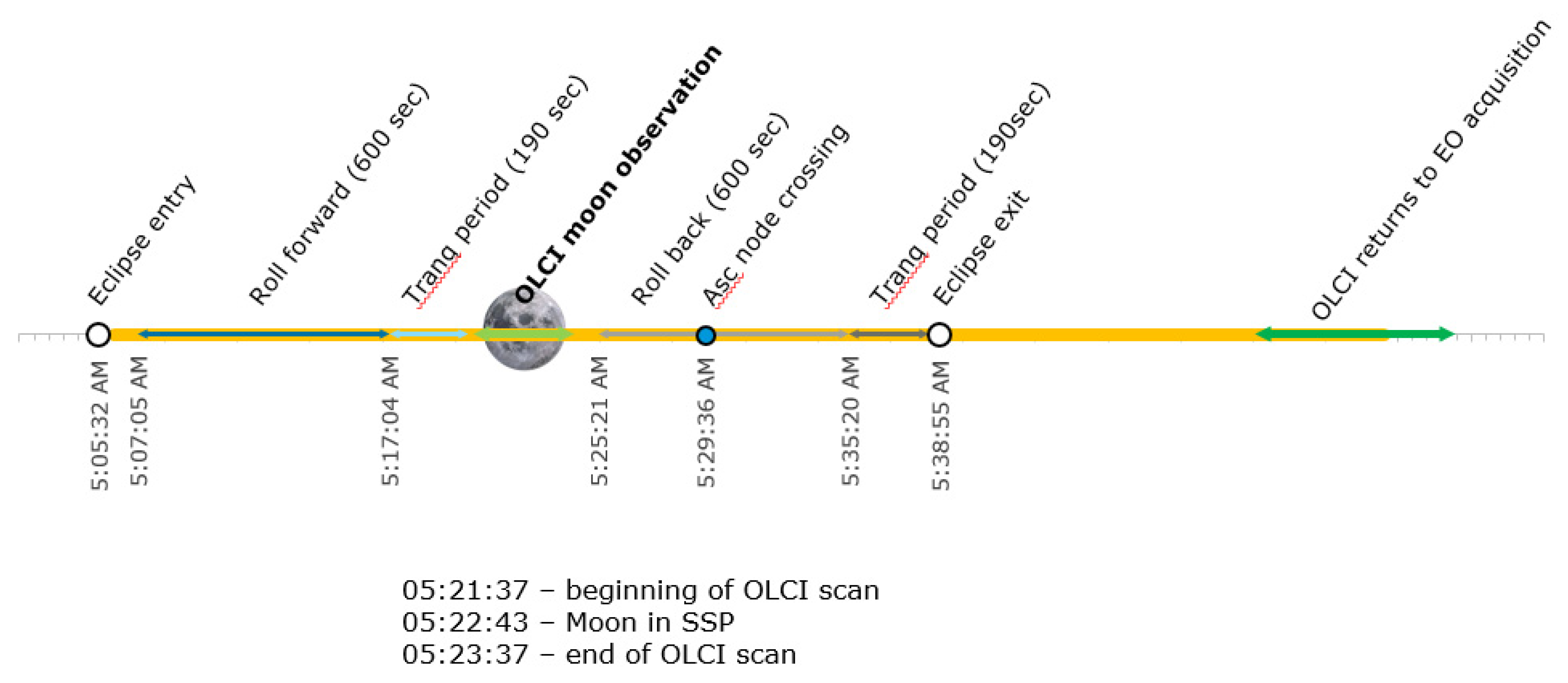
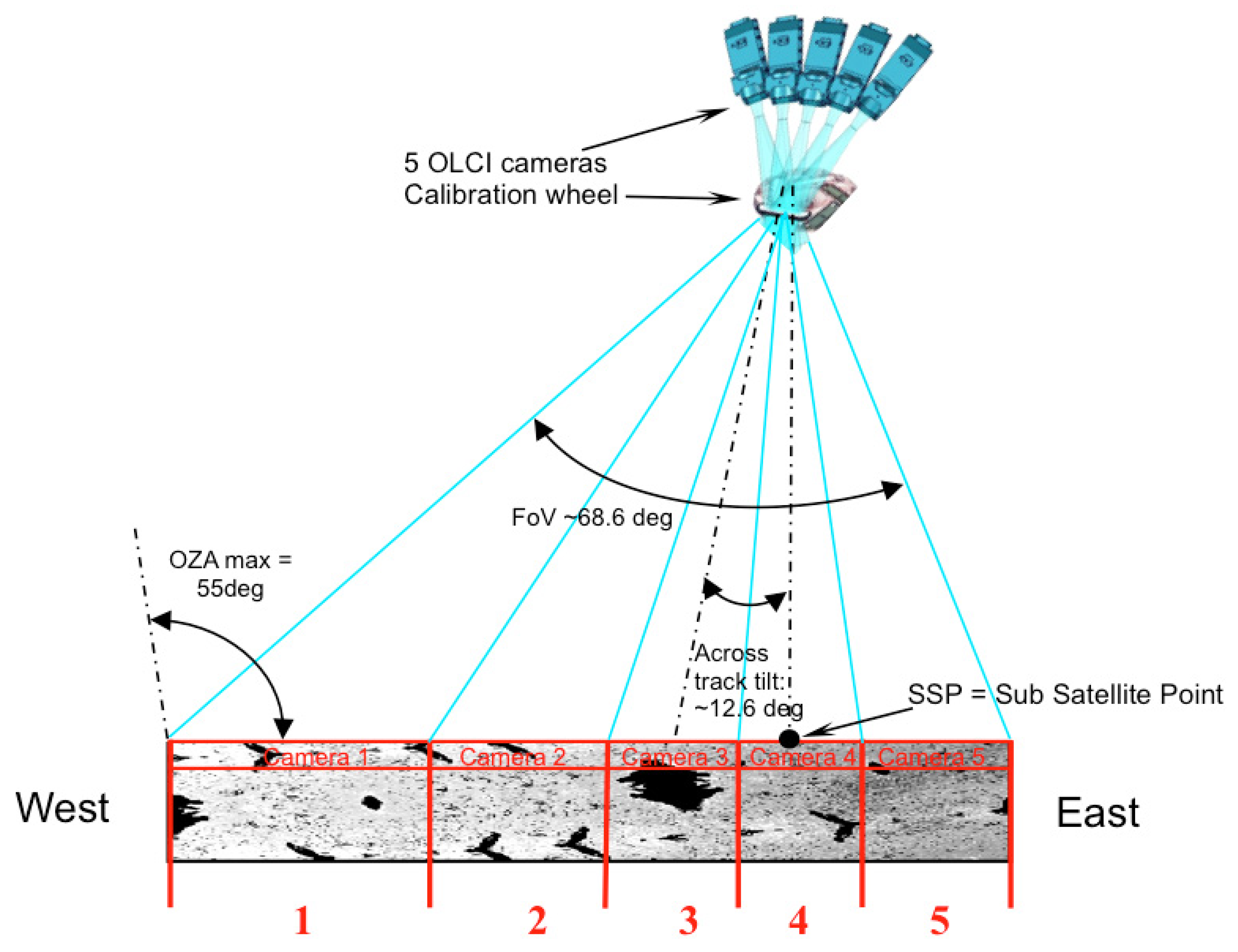
After the roll of the spacecraft was stabilized, the instrument was turned on in nominal Earth Observation mode. The instrument was collecting samples for 2 min with the moon coming into view roughly in the middle of this period with a phase angle of −6.45°. The timeline of the maneuver is presented in Figure 2. The calibration window was selected to make sure that the moon was as close to the middle of the swath as possible to avoid possible negative effects that may occur close to edges of the camera field of view (FOV). Additionally, one of the objectives was to capture all possible stray-light pixels.

Raw data (in Digital Numbers—DNs) acquired during the observation needs to be corrected and calibrated to physical values—undergo Level-1 processing. During processing, raw counts of the detector are converted to radiance as follows:

$$L_{b,k,m}=\frac{1}{A_{b,k,m}}\left(N{L}_{b,m,k}^{-1}\left[X_{b,k,m}\right]-S{m}_{b,k,m}\left(L_{*k,m}+SL\left(L_{*,*,*}\right)\right)-C_{b,k,m}\right)-SL\left(L_{*,*,*}\right)$$

(1)

where:

• $b, k, m$ subscripts stand for the spectral band, the spatial pixel, and the camera identifiers, respectively. When $*$ is used, it means that all items within the range are involved;
• $L_{b,k,m}$ is the scene radiance as seen by the pixel $b, k, m;$
• $X_{b,k,m}$ is the OLCI raw sample—in the equation, it is corrected for nonlinearity;
• $N{L}_{b,k,m}$ is a nonlinear function representing the nonlinearities within the video chain. It also depends on the VAM programmable gain $g$;
• $A_{b,k,m}$ is the instrument radiometric gain expressed in counts per radiance unit. It is determined in flight through the periodic radiometric calibration (performed with solar diffuser);
• $SL$ is the stray-light radiance contribution. It may result from all the wavelengths the detector is sensitive to, from the whole camera FOV (across-track) as well as from out of the FOV (i.e., from FOV of other modules, but also from FOV along-track, i.e., from scenes that have been previously observed or that will be further observed, hence the subscript $L_{*,*,*};$
• $S{m}_{b,k,m}$ is the smear contribution (light integration during Charge-Coupled Device (CCD) frame transfer);
• $C_{b,k,m}$ is the dark signal of the $b, k, m$ pixel during the observation.

The radiometric model is described in technical guides available at [16].

Since the radiometric model is valid regardless of the observed scene, this calibration approach holds for an OLCI moon observation. However, the processing chain was designed for Earth Observation without plans to perform moon observations routinely. Some steps of Level-1 processing are not applicable to data acquired from the moon scan. An obvious example of such a processing step is the georeferencing of samples. For that reason, a development platform of the Instrument Processing Facility (IPF-D) was used to process the moon data. It was configured to output partial Level-1 products, such as calibrated instrument radiances (before and after stray-light correction).

In the case of a wide field of view imaging spectrometer, such as the OLCI, in some observation scenarios (cloud-free ocean pixels close to clouds or land covered by vegetation), stray-light might significantly contribute to radiances. This issue is addressed with stray-light correction performed during Level-1 processing. The moon seen by Sentinel-3 instruments is (in visible bands) a bright circle on a nearly complete black background. This kind of sharp dark → bright → dark transition can be the perfect target to analyze stray-light [17,18,19]. Moon observation has proven to be a great opportunity to assess stray-light correction on-orbit.

2.2. OLCI Stray-Light and Its Correction

According to the OLCI design, the two main contributors to stray-light are the two main optical components, the ground imager and the spectrometer. Stray-light occurring within the ground imager consists of a two-dimensional process, related to the two spatial dimensions, namely the along-track and the across-track directions. There is an important assumption of lack of exchange between wavelengths, as there is no identified process implying energy transfer in the spectral dimension of the incoming radiance field inside the ground imager (GI). Contribution from the spectrometer is also a two-dimensional process with only one spatial dimension—the entrance slit aligned with the across-track dimension, canceling the along-track one and the spectral one introduced by the light dispersion device, the grating. In contrast with the ground imager, the spectrometer stray-light also includes a contribution from the sensor—a CCD—within which scattering of photoelectrons occurs and becomes significant at wavelengths higher than 900 nm.

OLCI stray-light correction was designed based on preliminary characterization showing moderate levels of stray-light—a few percent of the total signal. Therefore, it is assumed that the fundamental structure of the signal is preserved (even if it is slightly blurred by the stray-light) both from a spatial and spectral point of view. This allows using a robust correction method based on a second degradation of the signal. It is assumed that the second degradation has roughly the same impact on the (already) degraded signal as the actual sensing had on the original signal. As the system response is known, it is possible to degrade a second time the measured signal and, by subtraction, to estimate the degradation itself and correct for it. This is equivalent to the well-known expansion:

$${\left(1+\epsilon \right)}^2=1+2\epsilon +{\epsilon }^2\simeq 1+2\epsilon$$

(2)

Rewriting this for a stray-light degradation (linear) operator, the degraded version of the incoming signal x can be written as the sum of the original signal and the degradation itself:$\widehat{x}=x+\tilde{x}$.

The second degradation applied to the result gives:

$$\widehat{\widehat{x}}=\left(x+\tilde{x}\right)+\widetilde{\left(x+\tilde{x}\right)}=x+2\tilde{x}+\tilde{\tilde{x}}$$

(3)

If the degradation operator can be considered as a perturbation (in the physics sense)—that is verifying: energy($\tilde{x}$) << energy(x)—it follows: $\widehat{\widehat{x}}\approx x+2\tilde{x}$ as $\tilde{\tilde{x}}$ can be neglected and x can be retrieved by:

$$x\approx \widehat{\widehat{x}}-2\widehat{x}$$

(4)

This method is sometimes referred to as the “second degradation method”, described in detail in OLCI Level 1 Algorithm Theoretical Basis Document [20].

2.2.1. The Moon, a Great Target for Investigation on SL Correction

The OLCI-B moon observation has been used to assess the performance of the stray-light correction.

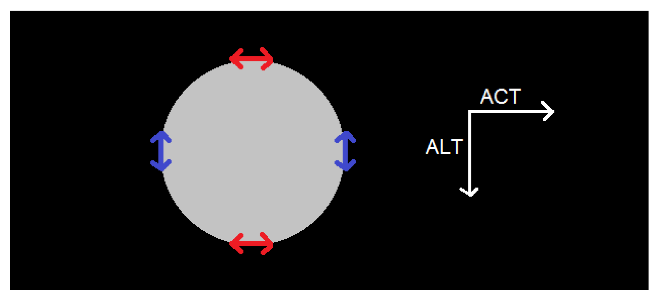
For several reasons, the moon is appropriate for stray-light analysis. First, there is in all spectral bands a sharp transition between bright and dark zones (respectively, moon and deep space), which is very important to analyze the impact of SL correction close to the bright/dark transitions. Second, the dark zone (deep space) is a homogeneous absolute reference at zero radiance, not perturbed by any geophysical signal. Third, the (near) full moon image allows selecting dark/bright interfaces aligned either with the ALT (along-track) direction or with the ACT (across-track) direction, as illustrated in Figure 3. This is important to help to separate the impact of GI (ground imager) SL from the impact of SP (spectrometer) stray-light, since in the ALT direction, only GI stray-light is active. Neglecting the curvature of the moon over a few lines or a few columns allows averaging these lines or columns to reduce the noise. Finally, the stray-light correction performance in the ALT and ACT directions can be assessed on both sides of the moon disk (above and below, left and right), which is important since the stray-light kernels are not systematically symmetrical (especially some ghosts which are present only on one side).

These conditions, well adapted for stray-light analysis, are difficult to find on Earth observation scenes.

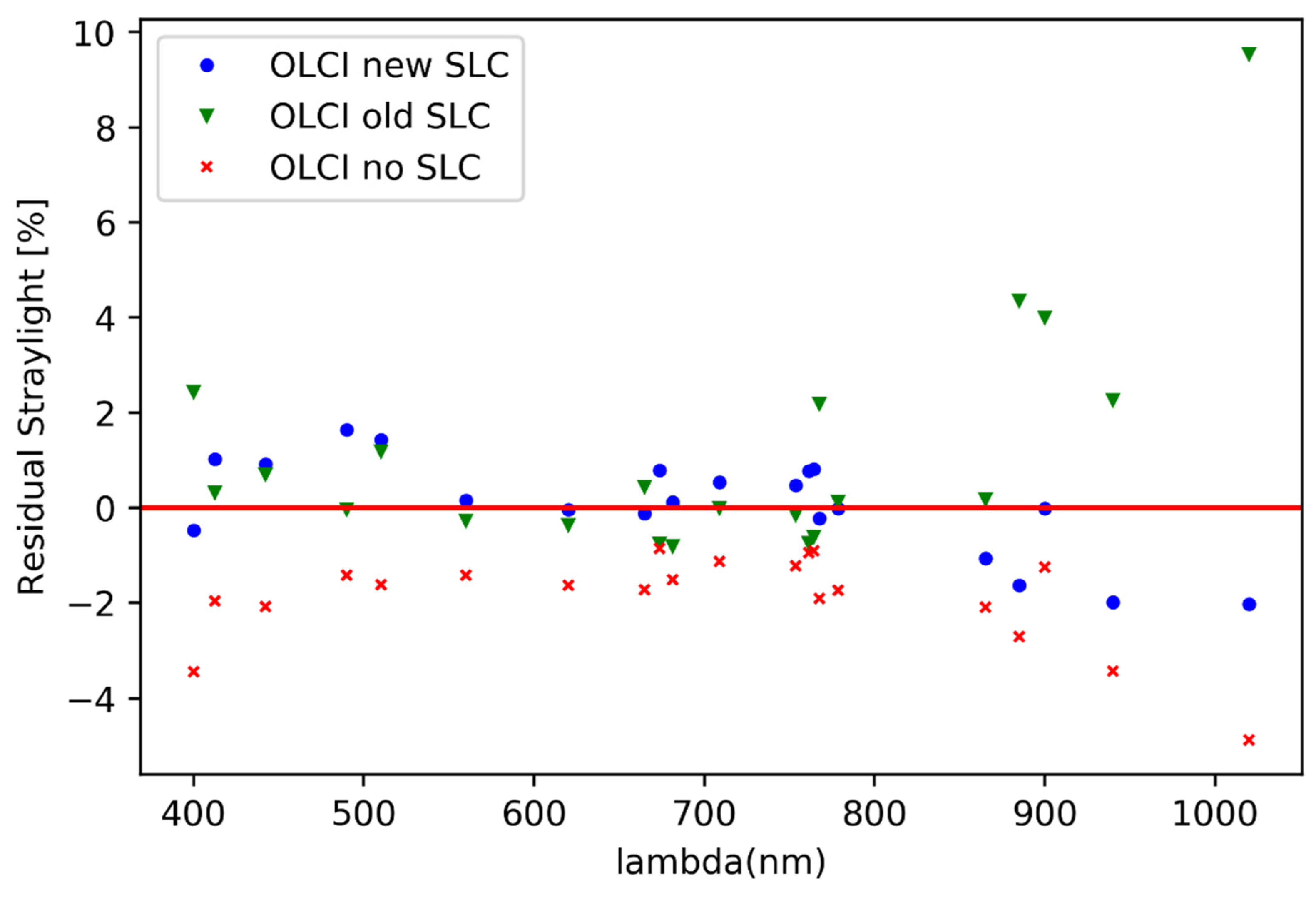
2.2.2. Potential SL Correction Improvements Tested on the Moon Data

The appropriateness of the moon scene for the stray-light investigations allowed us to test two potential improvements in the stray-light correction:

• An iterative method, a solution to the ε² limitation that appeared necessary for Near Infrared (NIR) bands
• Additional spectrometer SL kernels at wavelengths above 1000 nm, improving correction of channel Oa21, for which photoelectrons scattering inside the CCD is currently underestimated.

Iterative Method

As mentioned in Section 2.2, the stray-light correction relies on the “second degradation method”. This method is expected to work well when the stray-light is very small compared to the uncorrupted signal. In the NIR (typically spectral bands Oa19 to Oa21), the photoelectron scatter stray-light level becomes high, and the “second degradation method” results in a stray-light overcorrection.

In theory, this limitation of the “second degradation method” (also referred to as “ε² limitation”) for high stray-light levels can be improved by an iterative approach. It consists after a first estimation of the stray-light corrected radiance in re-estimating the stray-light by applying the SL kernel on this SL-corrected radiance, providing a better stray-light estimation since it is obtained from an image that has less stray-light. This re-estimated stray-light is then removed from the original image. This process can be performed iteratively, each iteration delivering a better estimation of the stray-light that should converge toward the true stray-light.

Practically, this “iterative” method can be achieved with no-extra computational cost by using a simple re-formulation of the kernels in the Fourier transform domain.

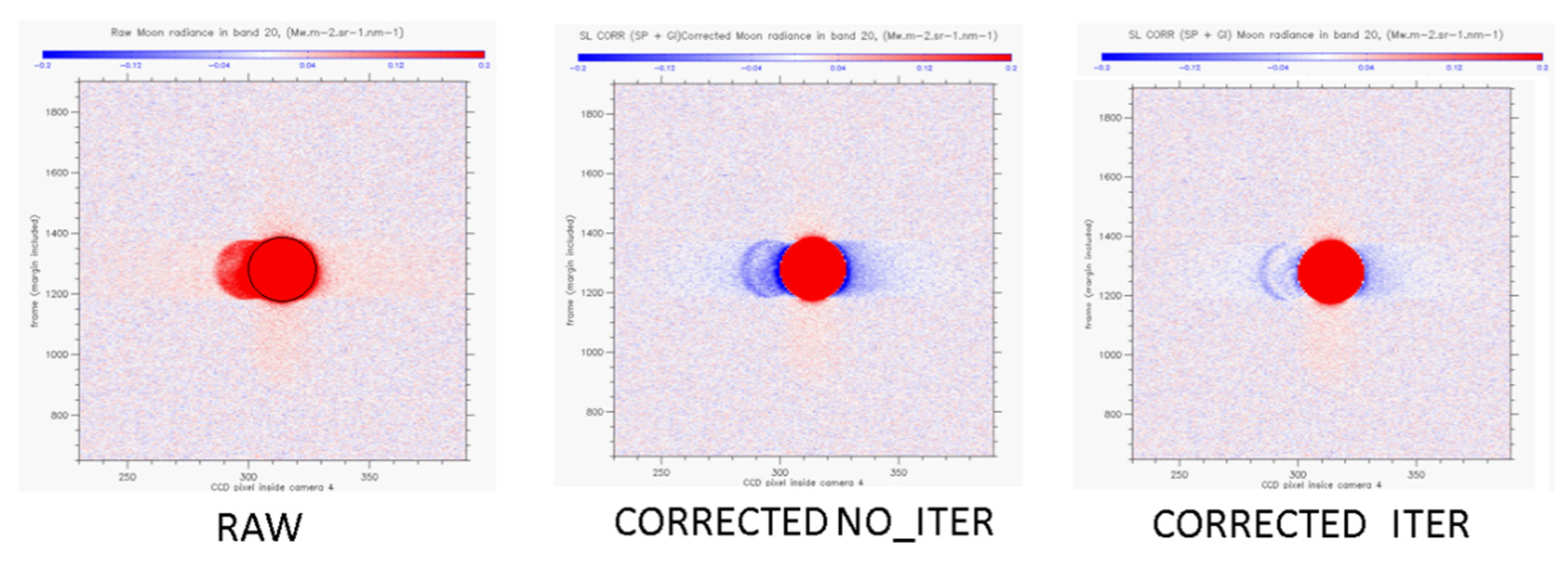
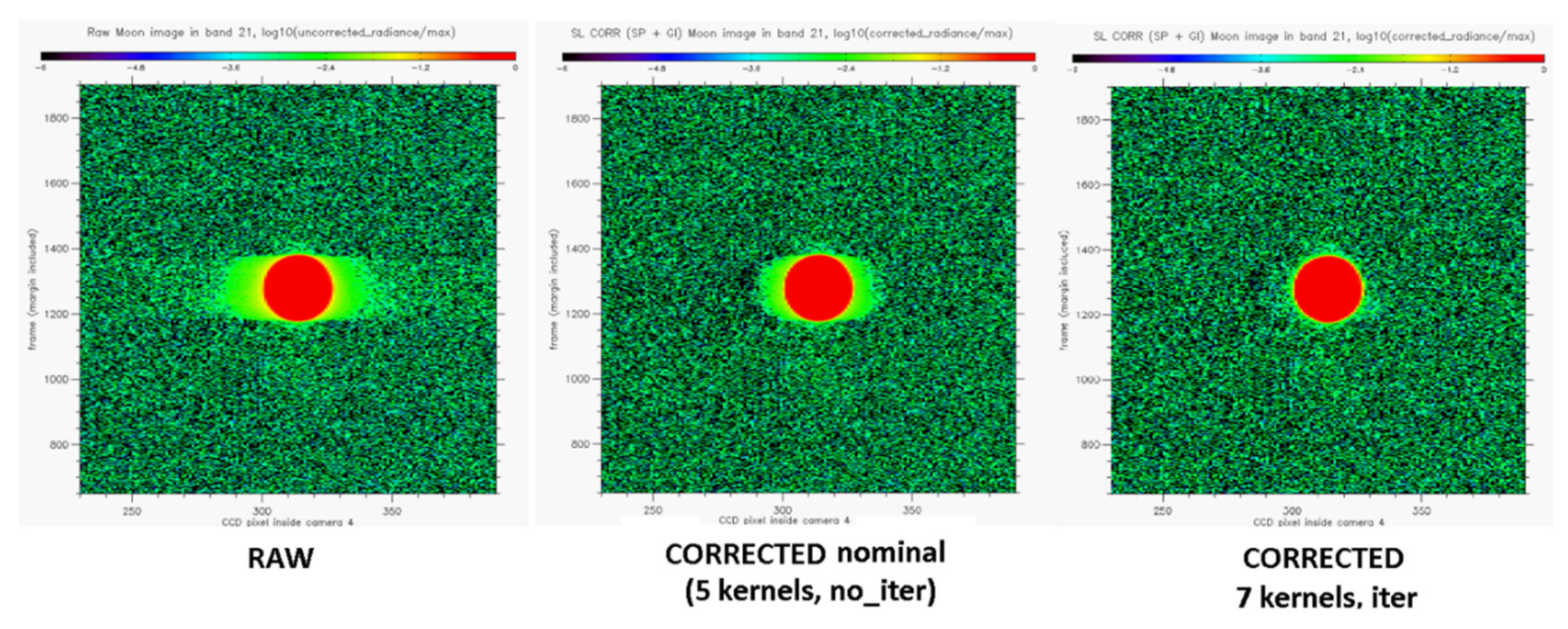
Tests on the moon data have shown, as expected, significant improvement in the NIR bands. This is illustrated for the band Oa20 (Figure 4) in which the overcorrection due to the “second degradation method” has been significantly reduced, even though a slight overcorrection remains, which may be due to other problems than the ε² limitation, such as characterization problem or interpolation problem.

Usage of Additional Spectrometer Stray-Light Kernel Above 1000 nm

In the NIR domain, one strong contributor to the total stray-light is the scattering of the photoelectrons within the CCD (so-called “NIR scatter” stray-light). This scattering is not an electronic cross-talk but an optical diffusion in the silicon layer of CCD. Photons with longer wavelengths are weakly absorbed within CCD material and diffuse to neighboring pixels. The NIR scatter stray-light is completely negligible below ≈900 nm but strongly and gradually increases toward longer wavelengths, reaching a maximum around 1028 nm, followed by a slight decrease until 1040 nm, the upper limit of OLCI’s spectral range. The NIR scatter stray-light contribution is accounted for in the spectrometer stray-light kernels, together with the optical contributions (scatter and ghost).

The nominal SL correction uses spectrometer kernels characterized at five different wavelengths. The last one is located at 973 nm, while the center of band Oa21 is around 1020 nm. Thus, its stray-light correction fully relies on the kernel at 973 (there is no extrapolation beyond characterization wavelengths). Consequently, the NIR_SCATTER stay-light is strongly underestimated for channel Oa21, resulting in significant residual NIR scatter stray-light in the corrected radiances.

To solve this problem, 2 stray-light kernels at 1028 nm and 1039 nm were added, corresponding respectively to the maximum of the NIR scatter curve and to the upper wavelength edge of band Oa21.

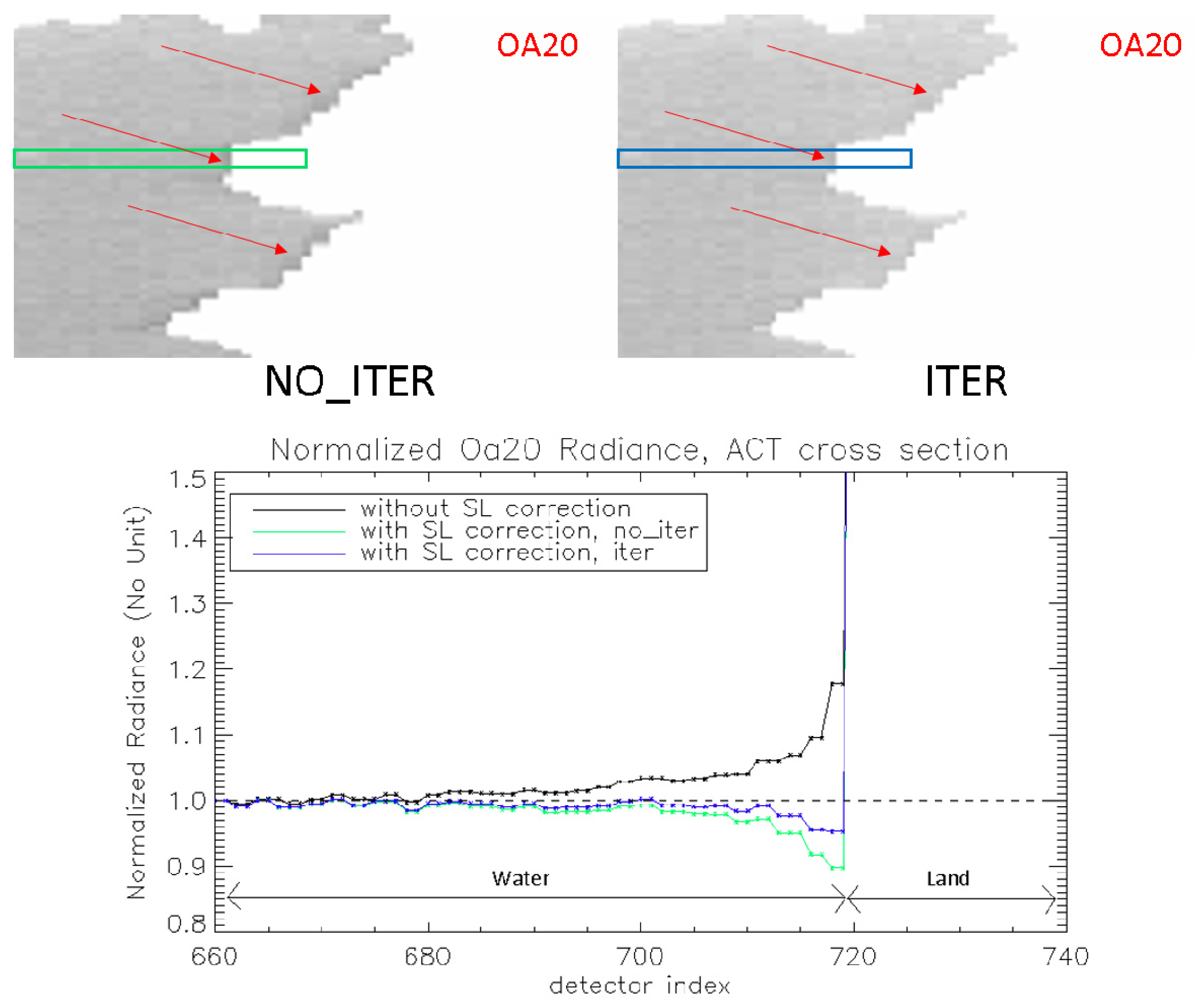
Stray-light correction was tested with these two additional kernels on the moon data, and very promising results were obtained, especially when coupled with the iterative method (described above). As illustrated in Figure 5: the green ACT pattern present on both sides of the moon (left plot, left and right of the moon disk) is residual NIR scatter stray-light: it almost completely disappears when using seven kernels and iterative method (right plot).

2.2.3. Possible Improvements to Earth Observation Data

In Section 2.2.2, the positive impact on moon data of the SL correction improvements (iterative method and additional kernels) was presented. Even though stray-light correction performance assessment is more difficult (especially quantitatively) on Earth Observation (EO), the new methods on EO scenes were applied and provided evidence of the expected improvements.

Figure 6 illustrates the improvement brought to Oa20 by the iterative method applied on an OLCI-A Earth Observation. It shows that, as for the moon observation, overcorrection next to the ACT bright/dark transition (here water/land) was significantly reduced.

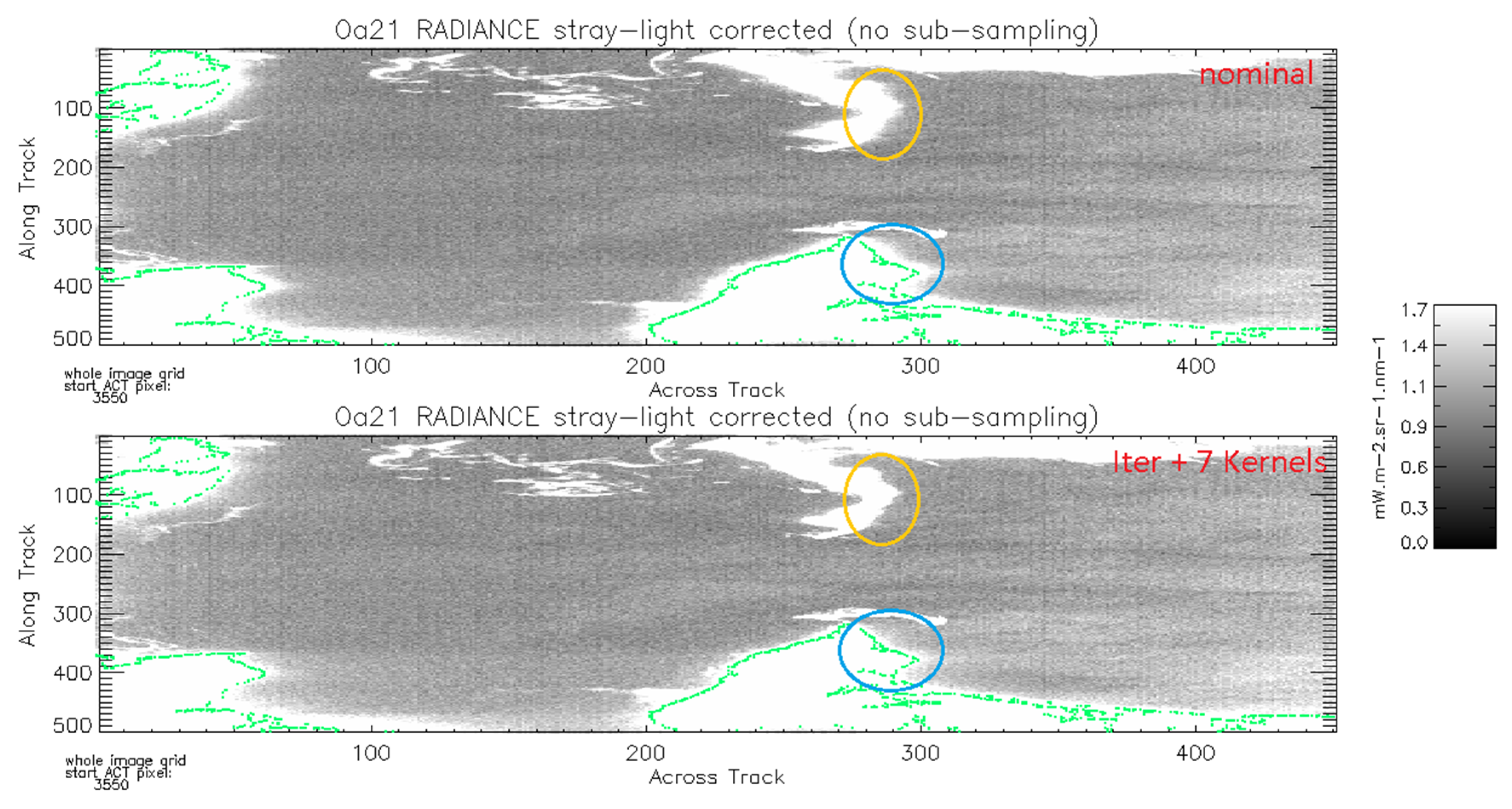
Figure 7 illustrates the improvement brought to band Oa21 by the two additional kernels when applied on an OLCI-B Earth observation. It shows that, as for the moon observation, ACT residual NIR scatter stray-light (thus an SL undercorrection) next to the ACT bright/dark transition (here land/water and cloud/water) was significantly reduced when considering the additional kernels (combined with the iterative method). One can see that the additional kernels at 1028 nm and 1039.75 nm allowed decreasing the residual NIR-scatter stray-light. Indeed, one can see in this image that:

• The location of the transition between the bright and dark pixels in the land/water interfaces was now closer to the coastline (see blue circle as an example).
• The transition between bright and dark pixels in the cloud/water interface became sharper (see orange circle as an example).

2.3. Oversampling of Moon Data

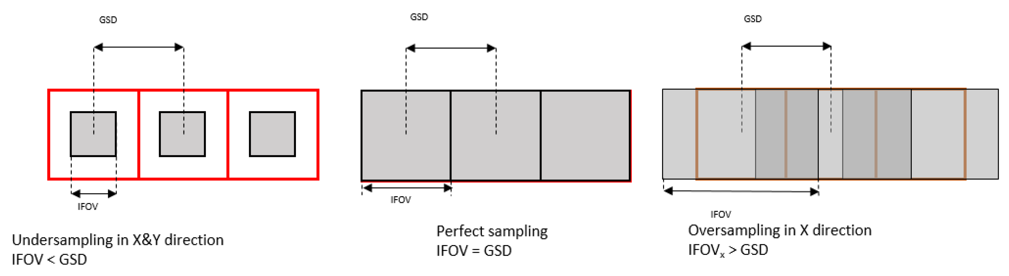
OLCI has been designed to observe the Earth from a specific orbit, at a specific spatial resolution, with a specific internal clock for the acquisitions. The distance between the spacecraft and the moon is much larger than the distance between the satellite and the Earth, which causes the lunar acquisitions to be oversampled as the satellite flies at its nominal speed. Oversampling (Figure 8) is a phenomenon that occurs when the distance between the centers of neighboring pixels (ground sampling distance—GSD) is smaller than the pixel instantaneous field of view (IFOV).

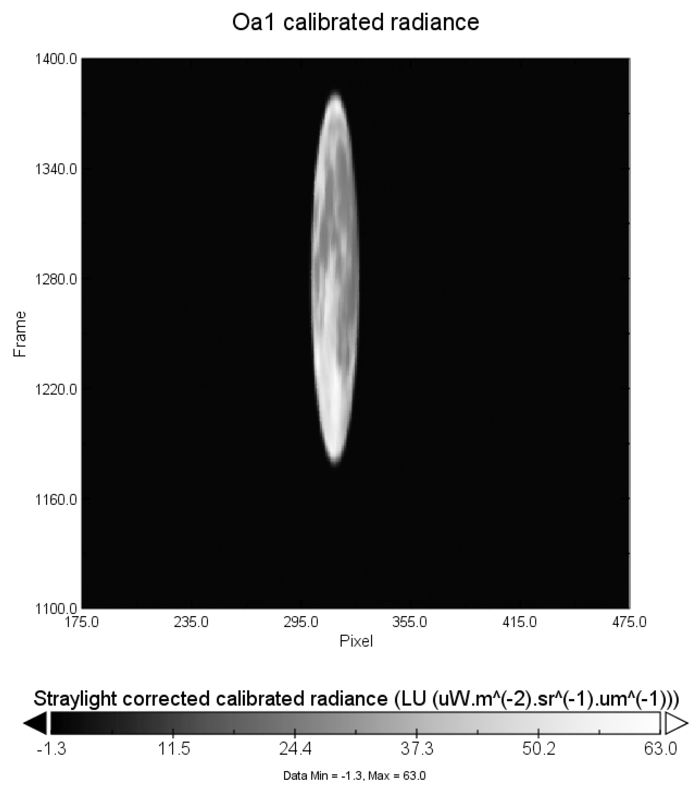
OLCI moon observation data is oversampled in flight (along-track—ALT) direction; the moon appears as elongated ellipse (Figure 9). Since the instrument is essentially a scanner, the along-track dimension of the image is built by satellite motion; the sampling time must be tuned to “match” the velocity of the satellite. This does not hold when observing the moon in nominal Earth Observation mode—the FOV diverges, while the orbital velocity and integration time (contributing to pixel pitch) remain the same. Since image in the across-track (ACT) direction is formed by the same array of detectors, their angular FOV and pixel separation remain the same, as during Earth Observation—there is no ACT oversampling. This instance of oversampling effect could be mimicked if we used an office scanner to scan a printed image of the moon, while slowly pulling the paper in the direction of scanners motion.

An accurate estimate of the oversampling factor is needed to both correct the image and analyze the radiance values. This estimate can be inferred from the orbit and instrument characteristics. Since the spacecraft completes one orbit in 100 min, the average angular velocity is $\frac{2\pi }{6000s}=1.047\frac{mrad}{s}$. During 44 ms (sampling time), the instrument covers an angular distance of 46 µrad. Compared to the distance between S3 and the Moon, the linear displacement of the satellite during this period is negligible, and this angle can be treated as the moon observation angular sampling step in ALT direction. When the instrument looks at the Earth, the subsatellite point (SSP) moves by a distance of $46 \mathsf{\mu }\mathrm{rad}\cdot 6380 \mathrm{km}=294 \mathrm{m}$. This linear pixel displacement seen from 814 km orbit forms angle $\beta =\frac{0.294km}{814km}=360 \mathsf{\mu }\mathrm{rad}$. The oversampling factor is the ratio of those two: $\frac{\beta }{\alpha }=\frac{360}{46}=7.83$.

This calculation can be expressed as:

$$O{S}_{factor}=\frac{\omega \cdot T_{sampl}\cdot R_{earth}}{H_{orbit}\cdot \omega \cdot T_{sampl}}=\frac{R_{earth}}{H_{orbit}}=7.83$$

(5)

where $\omega$ is the angular velocity of the spacecraft, $T_{sampl}$ is the sampling time, $R_{earth}$ is the mean Earth radius, and $H_{orbit}$ is the orbit height (above sea level). Most of the terms cancel out, and oversampling becomes a function of orbit height. This calculation of the oversampling ratio is assuming perfect sampling of Earth data form given orbit height. Based on a range of values of the calculated oversampling ratio derived with different parameters, the overall uncertainty is estimated at 2.5% of the calculated value.

It is important to notice that the instrument is assumed to sample from its orbit perfectly and that the moon is assumed to be sufficiently far to neglect displacement of the instrument between consecutive frames.

The oversampling factor is sometimes estimated using an ellipse fitting algorithm to fit the moon shape. However, this approach is not recommended [18] even for high illumination conditions as the fitting procedure parameters (e.g., the threshold on the quantization), as well as potential artifacts in the image, such as stray-light or ghosts, may lead to erroneous estimates of the oversampling factor. During this activity, ellipse fitting was only used to locate the moon and to automatically find the region of interest on the lunar scan and delimit the area of irradiance integration to the moon disc (with an additional fringe to ensure all moon pixels were included).

2.4. Irradiance Calculation

To assess the inflight radiometric performance of an instrument that has acquired lunar imagery, actual observations have to be compared to models. Such models spectrally simulate the moon signal for the specific geometrical conditions of the acquiring instrument at the time of the observation. Community reference models like ROLO) or GIRO estimate the reflectance spectrum of the moon as a function of time and satellite position and infer the lunar irradiance at instrument entry based on the solar irradiance. The observed lunar irradiance is estimated by integrating the lunar radiances recorded by the instrument.

Spectral irradiance is the integral of spectral radiance over a given surface.

$${\mathrm{E}}_{\mathsf{\lambda }}={{\displaystyle \int }}_{\mathsf{\Omega }}{L}_{\lambda ,x,y} d\mathsf{\Omega }$$

(6)

where ${\mathrm{E}}_{\mathsf{\lambda }}$ is the spectral irradiance coming from an area delimited by $\mathsf{\Omega }$—solid angle of the integrated surface, $L_{\lambda ,x,y}$ is the spectral radiance coming from point (x, y). In the case of discrete spectral radiances recorded by OLCI, integration is replaced by summation. Summation is performed over a range of points $n=1,2,3\dots$ that contribute to surface $\mathsf{\Omega }$. The infinitesimal solid–angular increment $d\mathsf{\Omega }$ is replaced by ${\omega }_n$—IFOV solid angle related to sample n.

$$E_{\lambda }=\frac{1}{O{S}_{corr}}{\displaystyle \sum }_n{L}_{\lambda ,n}\cdot {\omega }_n$$

(7)

A spectral radiance product of IPF-D was used in this study. It provided radiance values for each pixel in each scan of each band, corrected for effects normally influencing readouts during any observation (e.g., smear, nonlinearity, and stray-light). Values were corrected for oversampling ($O{S}_{corr}$) and appropriate IFOV values were assigned to each CCD pixel (${\omega }_n$).

The IFOV solid angle of a pixel can be estimated based on the ground pixel size. If we assume nadir pixel is 272 m ACT and 294 m ALT, and spacecraft is on 810 km orbit, the IFOV can be estimated as surface area divided by distance square:

$${\mathsf{\omega }}_{nadir}=\frac{Pi{x}_{ACT}\cdot Pi{x}_{ALT}}{R^2}=1.22\cdot {10}^{-7}sterad$$

(8)

Valid for the central pixel of the CCD. A more accurate value can be calculated based on the detector pixel pitch and focal length. If we take focal length f = 67.3 mm and pixel pitch ν = 0.0225mm (from instrument specification), we can calculate FOV in both directions: ACT—$a_x=2\cdot \mathrm{atan}\left(\frac{v}{2f}\right),$ ALT—$a_y=\mathrm{atan}\left(\frac{v}{f}\right)$.

This results in a solid angle: ${\omega }_{nadir}=a_x\cdot a_y=1.12\cdot {10}^{-7}sterad$

ACT IFOV of pixel n (counting from the middle of CCD) can be calculated as ACT IFOV of n pixels minus ACT IFOV of n-1 pixels: $a_x=\mathrm{atan}\left(n\cdot \frac{v}{f}\right)-\mathrm{atan}\left(\left(n-1\right)\cdot \frac{v}{f}\right)$. ALT IFOV was limited by spectrometer slit and was assumed to be constant—simulated differences were lower than 0.2%.

The most accurate value of detector IFOVs was based on ground tests and simulations performed during instrument assembly and acceptance (Figure 10). The uncertainty of the IFOV solid angle was estimated based on test requirements at 1.4%.

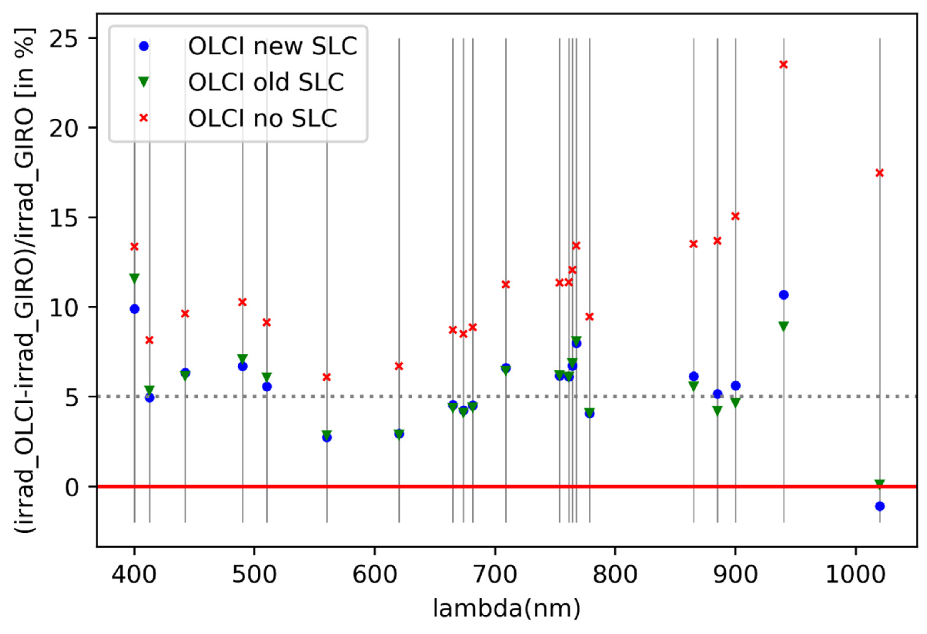
After accounting for oversampling and solid angle, the scene irradiance can be calculated and verified against a lunar irradiance model. It is worth pointing out that OLCI data is radiometrically calibrated by a ground data processor (IPF) that applies calibration inferred from an onboard solar diffuser, providing Level 1b radiance product. At instrument level, calculation of the observed irradiance reduces to a summation of radiances inside the moon disc (multiplied by respective solid angles) and correcting for oversampling. With this approach, any discrepancy between modeled irradiance and calculated instrument irradiance can indicate imperfection in processing chain or instrument radiometry (within the uncertainty range of modeled irradiance).

2.5. The GIRO Model

The GIRO model [10] has been developed by EUMETSAT in collaboration with United States Geological Survey (USGS). It has been endorsed by the Lunar Calibration Community, which encompasses the GSICS Research Working Group and the Comitee on Earth Observation Satellites (CEOS) Working Group on Calibration & Validation (WGCV) Infrared and Visible Optical Sensors Subgroup (IVOS), as the common lunar calibration reference model [17,18].

It is an implementation of the ROLO model [5] where the lunar disk reflectance, within the interval [350 nm, 2500 nm], is described by the following equation:

$${lnA}_k={\displaystyle \sum }_{i=0}^3{a}_{ik}{g}^i+{\displaystyle \sum }_{j=1}^3{b}_{jk}{\Phi }^{2j-1}+c_1\theta +c_2\varphi +c_3\Phi \theta +c_4\Phi \varphi +d_{1k}{e}^{-\frac{g}{p_1}}+d_{2k}{e}^{-\frac{g}{p_2}}+d_{3k}\cos \left(\frac{g-p_3}{p_4}\right)$$

(9)

where $k$ denotes the wavelength band, $g$ is the absolute phase angle, $\theta ,\varphi$ are the selenographic latitude and longitude of the observer (spacecraft), and $\Phi$ is the selenographic longitude of the sun. Parameters $a, b, c, d, p$ were retrieved from a fitting procedure making use of the extensive dataset acquired by the ROLO telescopes over more than eight years. The GIRO implemented the coefficients available in [5].

Reflectance is converted to spectral irradiance as follows:

$$E_{\lambda }=A_k\cdot \mathsf{\Omega }\cdot \frac{E{S}_k}{\pi }$$

(10)

where $\mathsf{\Omega }$ is the solid angle of the moon, $E{S}_k$ denotes solar spectral irradiance in band $k$ (corresponding to wavelength $\lambda$).

The GIRO was validated against the ROLO on an extensive set of data acquired by the SEVIRI instrument aboard Meteosat-8, 9, and 10. Additional comparisons were successfully made with instruments such as MODIS aboard Terra and Aqua or Suomi NPP VIIRS for the First Joint GSICS/IVOS Lunar Calibration Workshop to consolidate this validation [17].

The GIRO provides the lunar irradiance for the reflective solar bands of the processed radiometer at the instrument level. The range of phases covered by the model was |2, 92| degrees, as for the ROLO. The current uncertainties of the GIRO model for absolute calibration were between 5% and 10%, following the assessment made for the ROLO model [21]. However, for stability monitoring, the estimated uncertainty achieved less than 0.5% and even closer to 0.1% for long time series with consistent high illumination conditions [7,21].

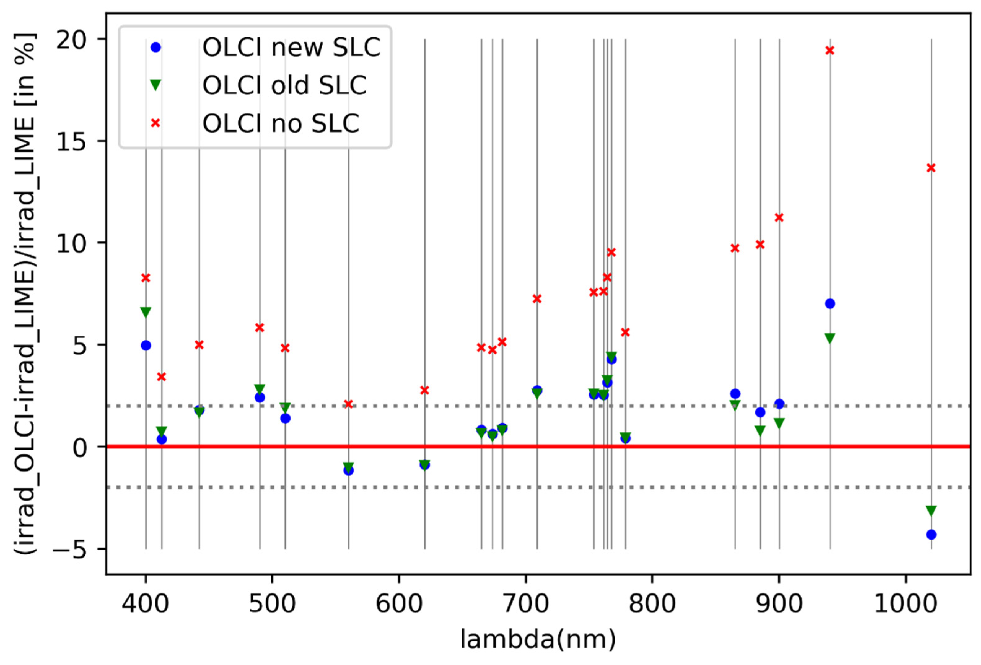
2.6. Lunar Irradiance Model ESA—LIME

In a recent project led by the National Physical Laboratory (NPL) in collaboration with the University of Valladolid and Flemish Institute for Technological Research (VITO) (funded by ESA), new lunar irradiance model—LIME (Lunar Irradiance Model ESA)—was developed.

LIME aimed at deriving an improved lunar irradiance model with sub-2% absolute radiometric uncertainty, SI traceable, based on new lunar observations carried out with a lunar photometer operated from the ground at the Pico Teide in Tenerife (Spain). The instrument was calibrated and characterized at NPL and operated from March 2018 to June 2019, providing around 150 useful nights of lunar observations that allowed deriving the first version of LIME. Additionally, wavelength dependency was introduced for several coefficients. The uncertainty analysis of the model output in the lunar photometer spectral bands led to an uncertainty of about 2% (k=2). Initial comparison to the GIRO model and a time series of EO satellite measurements (PROBA-V and Pléïades) was performed. A detailed description of the model and results of the comparison are available at 15. The photometer is still in operation. The model will be updated on a yearly basis based on an extended set of measurements.

In the current implementation of LIME, it provides lunar reflectance and irradiance at normalized distances. To compare instrument irradiance with LIME, it should be normalized to LIME geometry by following:

$$E_{\lambda }=f_d{E}_{\lambda }’, \mathrm{where} f_d={\left(\frac{D_{S-M}}{1 AU}\right)}^2{\left(\frac{D_{V-M}}{384400 km}\right)}^2$$

(11)

where $E_{\lambda }$ denotes spectral irradiance in LIME observation geometry, $E_{\lambda }’$ denotes spectral irradiance in satellite observation geometry, $D_{S-M}$ denotes the distance between the sun and the moon, $D_{V-M}$ denote the distance between the vehicle and the moon. This normalization is performed externally to reduce the number of regression parameters in the model.

3. Results and Discussion

This section will refer to three datasets obtained in different ways. The three datasets are:

• OLCI new SLC—dataset obtained with the improved stray-light correction described in Section 2.2. It is important to notice that radiometric gains in this variant were obtained using five kernel (old) implementation of SLC. The update is currently being implemented for gains calculation. The difference will be limited to band Oa21 and will result in approximately +2%–+3% higher gains. This change might improve results in Oa21.
• OLCI old SLC—dataset obtained with the current operational implementation of SLC.
• OLCI no SLC—dataset obtained as breakpoint mid-product before SLC correction. This is, however, still corrected for nonlinearity, dark offset, smear, and radiometrically scaled.

The detailed description of level 1 processing is provided in [22].

Instrument requirements specify radiometric uncertainty at 2% for wavelengths below 900 nm, 5% for longer wavelengths. An additional contributor to uncertainty was the uncertainty of the oversampling factor (estimated at 2.5%) and uncertainty of solid angle (IFOV) of detectors (specified at 1.4%). Overall, the uncertainty of measured irradiance was estimated at 3.5% for bands below 900 nm (Oa01-Oa18), 5.8% for bands above 900 nm (Oa19-Oa21).

LIME model delivers irradiance normalized to reference distances along with scaling factor that can be used to convert irradiance between observation distance and normalized distance. For the GIRO model, this conversion is already performed on output irradiance (it is provided as seen from the position of the satellite). For consistency, LIME values were scaled to satellite position by dividing them by $f_d$ from Equation (10).

3.1. Deep Space Offset

Since the moon was considered the only source of illumination of the acquired scene, we assumed the entire signal recorded by the instrument was coming from the moon—radiance contribution from stars was negligible. Therefore, additional verification of stray-light correction could be made based on the distribution of the signal on the full imagette. Ideally, the deep space signal (noise) should average to zero over any region of interest, and the sum of radiances of the whole imagette should be equal to the sum of the radiances inside the moon disc. However, it was noticed that the mean deep space level varies between bands (Figure 11).

While the relative level of deep space noise was very low, it is important to notice that there were around 4200 pixels inside the moon disk and 1.6 M pixels outside. To avoid bias, the inband average value of deep space pixels was subtracted from every pixel.

3.2. Spectral Behaviour

Radiances were limited to those inside the Moon disc, which was defined by an ellipse fitting algorithm and converted to mask array. Values in this mask array were one for every pixel inside ellipse-fitted moon disc; zero for every pixel outside. Then, this array was morphologically diluted with 5 × 5 kernel filled with ones, with three iterations. This caused the elliptical mask to grow in size, ensuring all moon pixels were included in calculations. Calculated instrument spectral irradiance was compared to LIME and GIRO models (Figure 12) to investigate the overall radiometric behavior of the instrument further. The models used the instrument mean spectral response functions (SRF) of each channel as provided in [22] instead of the SRF corresponding to the pixel viewing the moon center on Camera 4.

Both models predicted OLCI irradiance within their respective uncertainty ranges. There was a slight wavelength dependence between two models for short waves, maybe resulting from the fact that LIME introduced a number of wavelength dependencies to certain parameters. This interband behavior is better illustrated in Figure 13, where results were normalized to band Oa17. This way, all curves intersected at 865 nm with a relative value of one—bias between results was removed. Results showed a difference of about 5% between the models and the observations for bands Oa6 and Oa7 that were beyond the uncertainties on the oversampling and the solid angle calculation. It is also important to note that the change in curvature in band Oa20 (penultimate point—940 nm) visible in the models was absent from instrument data. Band Oa15 (767.5mn) also showed a different behavior between the models, which had a drop in irradiance, and the observed irradiance that had a much smoother trend. This behavior is not explained for now. To consolidate those results or to assess the temporal behavior of the instrument, more observations would be required.

3.3. Effect of Residual Stray-Light on Radiometric Accuracy

The relative bias between models and observations was calculated for the three mentioned datasets to assess the influence of the stray light correction on the integrated observed lunar irradiance. The stray-light model for OLCI is defined as not energy-conservative. Stray light is characterized by the use of ray tracing for two cases: ideal instrument with all photons not following direct path excluded and actual instrument including all photons on the direct path, as well as scattered and diffused photons. Stray-light is defined as the difference between those two cases. This means that the sum of irradiances in all bands (total energy) before and after SLC will be different. To achieve energy conservation in this comparison, radiometric gains for imagette before SLC should be derived from data without stray-light.

Calculated irradiances were also compared to models after dividing the bias by modeled irradiance:

$$\frac{Ir{r}_{modeled}-Ir{r}_{measured}}{Ir{r}_{modeled}}\cdot 100\%$$

(12)

This way, the interband behavior of instrument data with different SLC can be analyzed (Figure 14 and Figure 15).

The results with SLC (new and old) were very similar, with slight differences at higher wavelengths. Irradiance uncorrected for SLC was systematically higher—that is a result of the mentioned lack of energy conservation between those.

Measured irradiances were aligned closer to the LIME model. The majority of them were within the 2% uncertainty range. An overcorrection in Oa21 was likely causing a much lower level of this band.

Residual stray-light can be measured by comparing irradiance inside of the lunar disc to irradiance of complete imagette, so that:

$$Residual=\frac{Ir{r}_{disc}-Ir{r}_{img}}{Ir{r}_{img}}\cdot 100\%$$

(13)

For this analysis, the integration disk was tightened only to include moon pixels. Stray-light correction algorithms are optimized for the best performance of ground data processing. The very high contrast of the lunar scene causes strong overcorrection in pixels very close to the edge of the moon. This region (called no-requirement zone) was excluded by tightening the disc. This way, a comparison of plot Figure 16 shows the improvement in SLC in longer wavelengths.

4. Conclusions

While lunar observations were not envisioned as part of Sentinel-3 operations, a single observation was performed by the 3-B unit during commissioning to allow assessment of the potential benefits from this kind of maneuver. The acquired data set was subject to a number of internal studies performed at the European Space Research and Technology Centre (ESTEC), ACRI, and EUMETSAT that are presented here. While some aspects of the instrument can be characterized by a single observation (stray-light), the assessment of the radiometric performances and the temporal drift of the instrument would require regular observations. However, single observations still contribute to the overall understanding of the geometric and radiometric behavior of the instrument. Assessment of stray-light correction performed with the moon as target allowed improvement in SLC methodology. This improvement could be precisely tested on lunar observation data thanks to the characteristics of the scene (simple image with high contrast). Such conditions do not occur on the Earth scenes. Improved SLC mainly affects the long-wavelength channels, most notably significantly improving the performance of band Oa21. Calculated instrument irradiance was compared to lunar irradiance models. For most bands, the calculated irradiances were within a 2% uncertainty range of the LIME model. Currently, Sentinel-3A is preparing for a similar Moon Maneuver as for Sentinel-3B, i.e., performed in similar illumination and geometrical conditions (with the nadir Camera 4). Acquired data will provide an independent snapshot of the instrument radiometric status in the middle of its designed lifetime and may give an interesting insight into the aging of the subsystems.

References

1. Nieke, J.; Mavrocordatos, C.; Donlon, C.; Berruti, B.; Garnier, T.; Riti, J.B.; Delclaud, Y. Ocean and Land Color Imager on Sentinel-3. In Optical Payloads for Space Missions; John Wiley & Sons, Ltd.: Hoboken, NJ, USA, 2015; Chapter 10; pp. 223–245. [Google Scholar] [CrossRef]
2. Nieke, J.; Dransfeld, S.; Donlon, C.; Berruti, B.; Mecklenburg, S. SENTINEL-3 A and B optical payload: Early results from commissioning and tandem flight activities. In Proceedings of the International Geoscience and Remote Sensing Symposium (IGARSS), Valencia, Spain, 22–27 July 2018; Institute of Electrical and Electronics Engineers Inc.: Piscataway, NJ, USA, 2018; Volume 2018, pp. 1098–1099. [Google Scholar] [CrossRef]
3. Ando, S.; Tanaka, K. In-orbit stray-light characterization and correction of optical radiometer using the moon image. Mech. Eng. J. 2019, 6, 19-00098. [Google Scholar] [CrossRef] [Green Version]
4. Kieffer, H.; Wildey, R. Establishing the Moon as a Spectral Radiance Standard. J. Atmos. Ocean. Technol. 1996, 13, 360–375. [Google Scholar] [CrossRef] [Green Version]
5. Kieffer, H.H.; Stone, T.C. The Spectral Irradiance of the Moon. Astron. J. 2005, 129, 2887. Available online: http://0-iopscience-iop-org.brum.beds.ac.uk/1538-3881/129/6/2887/pdf/204408.web.pdf (accessed on 26 June 2020). [CrossRef] [Green Version]
6. Godden, G.; McKay, C. A Strategy for Observing the Moon to Achieve Precise Radiometric Stability Monitoring. Can. J. Remote Sens. 1997, 23, 333–341. [Google Scholar] [CrossRef]
7. Barnes, R.A.; Eplee, R.E.; Patt, F.S.; Kieffer, H.H.; Stone, T.C.; Meister, G.; Butler, J.J.; McClain, C.R. Comparison of SeaWiFS Measurements of the Moon with the U.S. Geological Survey Lunar Model. Appl. Opt. 2004, 43, 5838–5854. [Google Scholar] [CrossRef] [PubMed] [Green Version]
8. Xiong, X.; Sun, J.; Chiang, K.; Xiong, S.-J.; Barnes, W.L. MODIS on-orbit characterization using the moon. Proc. SPIE 2003, 4881, 299–307. [Google Scholar]
9. Stone, T.C.; Kieffer, H.H.; Grant, I.F. Potential for Calibration of Geostationary Meteorological Satellite Imagers using the Moon. Proc. SPIE 2005, 5882. [Google Scholar] [CrossRef]
10. Viticchiè, B.; Wagner, C.S.; Hewison, T.J.; Stone, T.C.; Nain, J.; Gutierrez, R.; Müller, J.; Hanson, C. Lunar Calibration of MSG/SEVIRI Solar Channels. In Proceedings of the AMS—EUMETSAT User Conference, Vienna, Austria, 16–20 September 2013. [Google Scholar]
11. Oh, T.H.; Kim, D. COMS Visible Channel Calibration Using Moon Observation Data. Remote Sens. 2018, 10, 726. [Google Scholar] [CrossRef] [Green Version]
12. Sun, J.; Xiong, X.; Barnes, W.; Guenther, B. MODIS Reflective Solar Bands On-orbit Lunar Calibration. IEEE Trans. Geosci. Remote Sens. 2007, 45, 2383–2393. [Google Scholar] [CrossRef]
13. Choi, T.; Shao, X.; Cao, C. On-orbit radiometric calibration of Suomi NPP VIIRS reflective solar bands using the Moon and solar diffuser. Appl. Opt. 2018, 57, 9533–9542. [Google Scholar] [CrossRef] [PubMed]
14. EUMETSAT Website. Moon as Reference for Long Term Stability Assessment of Optical Sensors. Available online: https://www.eumetsat.int/website/home/Data/ScienceActivities/ScienceStudies/Moonasreferenceforlongtermstabilityassessmentofopticalsensors/index.html (accessed on 26 June 2020).
15. CEOS Cal/Val Portal, Lunar Irradiance Model ESA: LIME. Available online: http://calvalportal.ceos.org/lime (accessed on 26 June 2020).
16. Sentinel online Website. OLCI Technical Guide. Available online: https://sentinel.esa.int/web/sentinel/technical-guides/sentinel-3-olci (accessed on 26 June 2020).
17. Wagner, S.T.; Hewison, T.; Stone, T.; Lacherade, S.; Fougnie, B.; Xiong, X. A summary of the joint GSICS—CEOS/IVOS lunar calibration workshop: Moving towards intercalibration using the Moon as a transfer target. SPIE Remote Sens. 2015, 9639. [Google Scholar] [CrossRef]
18. GSICS Wiki. Second Joint GSICS/IVOS Lunar Calibration Workshop in Xi’an (China), 13–17 November 2017. Available online: http://129.2.124.227/bin/view/Development/20171106 (accessed on 26 June 2020).
19. Summary of the Second Joint GSICS/IVOS Lunar Calibration Workshop, 13–17 November 2017, Xi’an, China. Available online: http://gsics.atmos.umd.edu/pub/Development/20171106/Summary%20-%20Second%20Lunar%20Calibration%20Workshop%20-%20Xian%202017.pdf (accessed on 26 June 2020).
20. Bourg, L. “OLCI Level 0, Level 1b Algorithm Theoretical Basis Document”, S3-ACR-TN-007 Issue 5.0. 10 December 2014. Available online: https://sentinels.copernicus.eu/web/sentinel/user-guides/sentinel-3-olci/document-library/-/asset_publisher/hkf7sg9Ny1d5/content/sentinel-3-olci-level-0-and-level-1b-atbd (accessed on 26 June 2020).
21. Stone, T.C.; Kieffer, H.H. Assessment of uncertainty in ROLO lunar irradiance for on-orbit calibration. In Proceedings of the SPIE 5542, Earth Observing Systems IX, Denver, CO, USA, 2–6 August 2004. [Google Scholar] [CrossRef]
22. Sentinel online Website. OLCI Instrument Specifications. Available online: https://sentinel.esa.int/web/sentinel/technical-guides/sentinel-3-olci/olci-instrument/specifications (accessed on 26 June 2020).
Figure 1. Basic Ocean Land Color Instrument (OLCI) geometry. Field of view (FOV) is tilted westward to avoid sun glint.
Remotesensing 12 02543 g001
Figure 2. Timeline of OLCI-B Moon Observation.
Remotesensing 12 02543 g002
Figure 3. Synthetic representation of the OLCI-B moon observation showing the interfaces between bright and dark zone, which are aligned with along-track (ALT) direction (blue arrows) or across-track (ACT) direction (red arrows).
Remotesensing 12 02543 g003
Figure 4. Oa20 moon radiance (left) without stray-light correction, (middle) after nominal correction, (right) after correction using the iterative method. Color scale is linear, centered on zero (deep space value) and limited to stray-light radiance levels (i.e., the moon disk is saturated); red is for positive, white for close to 0, blue for negative radiance. On the left plot, a black circle has been drawn to visualize the moon disk better.
Remotesensing 12 02543 g004
Figure 5. Oa21 moon radiance (left) without stray-light correction, (center) after nominal correction, (right) after correction using seven kernels and iterative method. Plotted radiances are normalized to maximum and log-scaled to highlight the stray-light impact on the deep-space background around the moon disk. It cannot be compared to that of Figure 4.
Remotesensing 12 02543 g005
Figure 6. Earth Observation stray-light corrected Oa20 radiance over part of the lake of Michigan where dark/bright (water/land) transition occurs (OLCI-A scene, 27/07/2017 15h35), (upper left) without iteration, (upper right) with iterations. The red arrows highlight some improvements brought by the iterative method. (bottom) ACT cross-section in the region of the image indicated by the rectangle (a few frames were averaged to reduce the noise). The curves were normalized by their radiance value at detector index 660 located in the water part at a significant distance from the water/land transition. The data without stray-light correction has been added in black.
Remotesensing 12 02543 g006
Figure 7. Earth Observation stray-light corrected Oa21 radiance in camera 4, in a region of the Gulf of Saint-Laurence where dark/bright (sea/land and sea/cloud) transitions occur. This measurement was done on 25 MAR 2020 ≈14h57 with OLCI-B. (top) nominal processing, (bottom) processing with iterations, and seven kernels. The green line represents the coastline. The yellow and blue circles give an example of where the improvement brought by the additive kernels (combined with the iterative method) happens. The orange and blue circles give examples of where the improvement happened (note, however, that it happened at all ACT bright/dark transition pixels).
Remotesensing 12 02543 g007
Figure 8. Different sampling conditions. Three ground pixels are equally spaced, however, depending on instantaneous field of view (IFOV) detectors, this scene might be over/under sampled.
Remotesensing 12 02543 g008
Figure 9. Radiance imagette from OLCI camera 4, band Oa1 moon scan shows the oversampling effect on moon data. Image is 300 × 300 pixels with ACT direction on X-axis.
Remotesensing 12 02543 g009
Figure 10. Variation of pixel IFOV along CCD. In observation performed in June 2018, the moon was imaged by pixels between red lines marked on the chart.
Remotesensing 12 02543 g010
Figure 11. Mean deep space levels relative to mean level inside moon disc.
Remotesensing 12 02543 g011
Figure 12. Comparison of absolute irradiance at satellite level with Lunar Irradiance Model ESA (LIME) and GSICS Implementation of Robotic Lunar Observatory (GIRO) models. Dash–dot envelopes indicate expected uncertainty ranges of the model.
Remotesensing 12 02543 g012
Figure 13. Irradiance normalized to band Oa17 (865 nm).
Remotesensing 12 02543 g013
Figure 14. Comparison of OLCI calculated irradiances (with different stray-light correction (SLC)) relative to the GIRO model.
Remotesensing 12 02543 g014
Figure 15. Comparison of OLCI calculated irradiances (with different SLC) relative to the LIME model.
Remotesensing 12 02543 g015
Figure 16. Residual stray-light in different SLC variants. Strong overcorrection of the longest wavelengths is replaced by slight undercorrection (negative values).
Remotesensing 12 02543 g016