Hyperspectral Image Classification Using Feature Relations Map Learning

School of Resource and Environmental Sciences, Wuhan University, Wuhan 430079, China
*
Author to whom correspondence should be addressed.
Remote Sens. 2020, 12(18), 2956; https://0-doi-org.brum.beds.ac.uk/10.3390/rs12182956
Submission received: 2 August 2020
/
Revised: 9 September 2020
/
Accepted: 9 September 2020
/
Published: 11 September 2020
Abstract
:Recently, deep learning has been reported to be an effective method for improving hyperspectral image classification and convolutional neural networks (CNNs) are, in particular, gaining more and more attention in this field. CNNs provide automatic approaches that can learn more abstract features of hyperspectral images from spectral, spatial, or spectral-spatial domains. However, CNN applications are focused on learning features directly from image data—while the intrinsic relations between original features, which may provide more information for classification, are not fully considered. In order to make full use of the relations between hyperspectral features and to explore more objective features for improving classification accuracy, we proposed feature relations map learning (FRML) in this paper. FRML can automatically enhance the separability of different objects in an image, using a segmented feature relations map (SFRM) that reflects the relations between spectral features through a normalized difference index (NDI), and it can then learn new features from SFRM using a CNN-based feature extractor. Finally, based on these features, a classifier was designed for the classification. With FRML, our experimental results from four popular hyperspectral datasets indicate that the proposed method can achieve more representative and objective features to improve classification accuracy, outperforming classifications using the comparative methods.
1. Introduction
As the spectral resolution of remote sensing (RS) sensors has improved, hyperspectral technology has exhibited great potential for obtaining land use information with fine quality. Hyperspectral RS images capture the spectrum of every pixel within observed scenes at hundreds of continuous and narrow bands. In comparison with multispectral images, which have wide wavelength, hyperspectral images can provide features hidden in narrow wavelengths in order to distinguish objects that are difficult to detect [1,2]. Since hyperspectral RS images have powerful capabilities, they have popularly been used in many fields, such as mining, precision agriculture, water pollution treatment, etc. [3,4,5].
Hyperspectral RS image classification is an important process for transforming hyperspectral information from the ground’s surface into attribute information. It is an extension of the conventional multiple spectral RS image classification, which aims at assigning a pixel to a unique class [6,7]. Hyperspectral images differ significantly from multiple spectral images because they have high-dimensional features and the correlation between adjacent bands is often high. Along with other aspects, such as noise and mixed pixels, hyperspectral image classification also suffers from data redundancy, dimensional disaster, and uncertainty, making this type of classification more complex and challenging [8,9].
Various methods have been proposed for hyperspectral RS image classification. Classification methods for traditional multiple spectral images, such as support vector machine (SVM), k-nearest neighbor (KNN), naive Bayesian (NB), and decision tree (DT), have early on been transformed into hyperspectral image classification [10,11]. However, influenced by the high data dimension, most of these methods have the drawback of accuracy improvement and are complexed in operation [9,11,12]. Thus, more advanced classifiers are needed to better fit hyperspectral image classification that typically include ensemble learning (EL), such as rotation-based deep forest, cascaded random forest, hybridized composite kernel boosting, canonical correlation forests, and other versions, have been reported as effective approaches to overcoming the shortage of high dimension data classification [8,13,14,15,16]. However, due to the complexity of spatial and spectral factors, the capability of classifier generalization still needs to be improved.
In addition to using advanced classifiers, reducing the complexity of hyperspectral data and extracting new features are other important approaches to improving classification accuracy. These methods focus on solving the classification problem though data processing methods. Up until now, many such methods have been proposed. One popular method is to convert the spectral vector of pixels into a low-dimensional feature space, such as principal component analysis (PCA), independent component analysis (ICA), regularized linear discriminant analysis, and Fisher discriminant analysis [17,18,19]. Another popular method is to extract features with filters that contain different discriminations, such as extended extinction profile, Gabor filters, scatting wavelet transform, and local binary pattern (LBP) [20,21,22]. All these methods have achieved excellent performance in different classification fields. However, most of them heavily depend on hand-crafted features, which are usually designed for a specific task and need a complex parameter setup phase, and the extracted features are not enough to discriminate the land use in more detail [7,23].
Deep learning (DL), a new breakthrough in machine learning (ML), is proven to be one of the most excellent RS classification methods. Unlike other classification methods, DL provides feature learning and deep architecture to model higher-level feature representations without human-designed features or rules [23,24,25]. Convolutional neural network (CNN), a very popular DL method, has produced state-of-the-art results for object detection and RS image classification. It focuses on bridging low-level features to high-level semantics of an image scene and on extracting the intrinsic features from RS images automatically [26]. Recently, CNNs have been reported to be one of the most effective methods for hyperspectral image classification and to show different points of view in their application, including spectral-based, spatial-based, and spectral-spatial based [27,28,29].
Spectral-based methods are conceptually simple and easy to implement, with most of them using one-dimensional CNN (1-D CNN) architectures to extract features from spectral bands. However, these methods ignore spectral contexts, resulting in an unsatisfactory classification performance [7,27]. Spatial-based approaches consider the neighboring pixels of a certain pixel within a scan to extract spatial information using two-dimensional CNN (2-D CNN) architectures. As they are more focused on spatial contexts, most of these methods use pre-processing methods, such as PCA and autoencoders, to first reduce image dimension—however, this process would lose some details in the spectrum, and reduce the capability of these methods to distinguish different objects [27,30,31]. Spatial-spectral approaches fuse the spatial and spectral information using three-dimensional CNN (3-D CNN) architectures and combining the advantages of both 1-D and 2-D CNNs. As they can learn features both in the spatial and spectral domains of hyperspectral cubes, the methods have received more and more attention in order to improve hyperspectral image classification quality in recent research [32,33,34].
CNN has powerful feature learning capability, which could provide more discriminative features for hyperspectral image classification with higher quality. If the learned features are more discriminative, then classification problems would be simpler to solve [35,36,37]. However, CNNs have shortcomings for extractions of global features because most of them extract features from hyperspectral images layer by layer using convolutional filters that cover the neighboring bands and pixels [7,23,32,38]. In addition, in hyperspectral image classification, the existing CNN based methods are focused on extracting hidden features from the spectral, spatial, or spatial-spectral domains [24,39,40], while the rich information that could be generated by the interactions between different original features are not fully considered. Thus, from a global perspective, utilizing all original features to establish relations between them and then learning the features from their relations would be a novel approach to discovering more intrinsic and representative features.
Beyond having the existing CNN methods learn features from original hyperspectral images, it is relatively rare to convert spectral or spatial information into regular texture pictures for feature learning with the CNNs. In fact, extensive literature reports that CNNs have more powerful capability to learn features from pictures with regular textures [26,41,42,43,44]. Therefore, it could be assumed that converting spectral information of each pixel in hyperspectral images into regular texture scan images and using CNNs for feature learning would greatly improve classification accuracy.
For the reasons given above, we propose a new approach—called feature relations map learning (FRML)—for improving hyperspectral image classification. Here, the feature relations mean the correlations between features under certain function or mapping. First, for a pixel on the image, the relations between each two spectral features are calculated by a specific function and are recorded using a 2-D matrix. Then, the matrix is converted into a picture, which can describe the relations between different spectral features with regular textures. Finally, new features are learned from the picture based on CNN architecture and the current pixel is classified and a predicted class label is signed. After FRML is performed on the entire image, a more accurate land use map is produced. Specifically, the remainder of this paper is organized as follows. Section 2 introduces FRML and related work. Section 3 describes data sets and experimental designs. In Section 4, we analyze the experimental results and present the discussion. Finally, conclusions and suggestions are provided in Section 5.
2. Methods
2.1. Feature Relations Map Learning
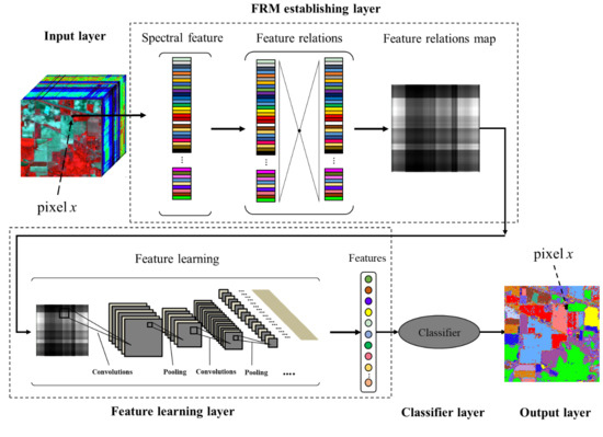
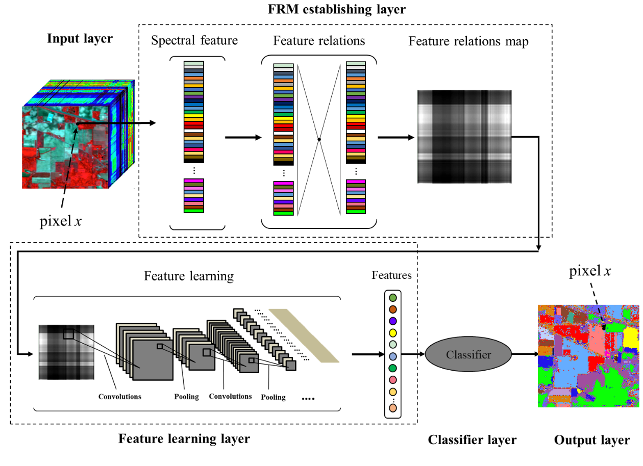
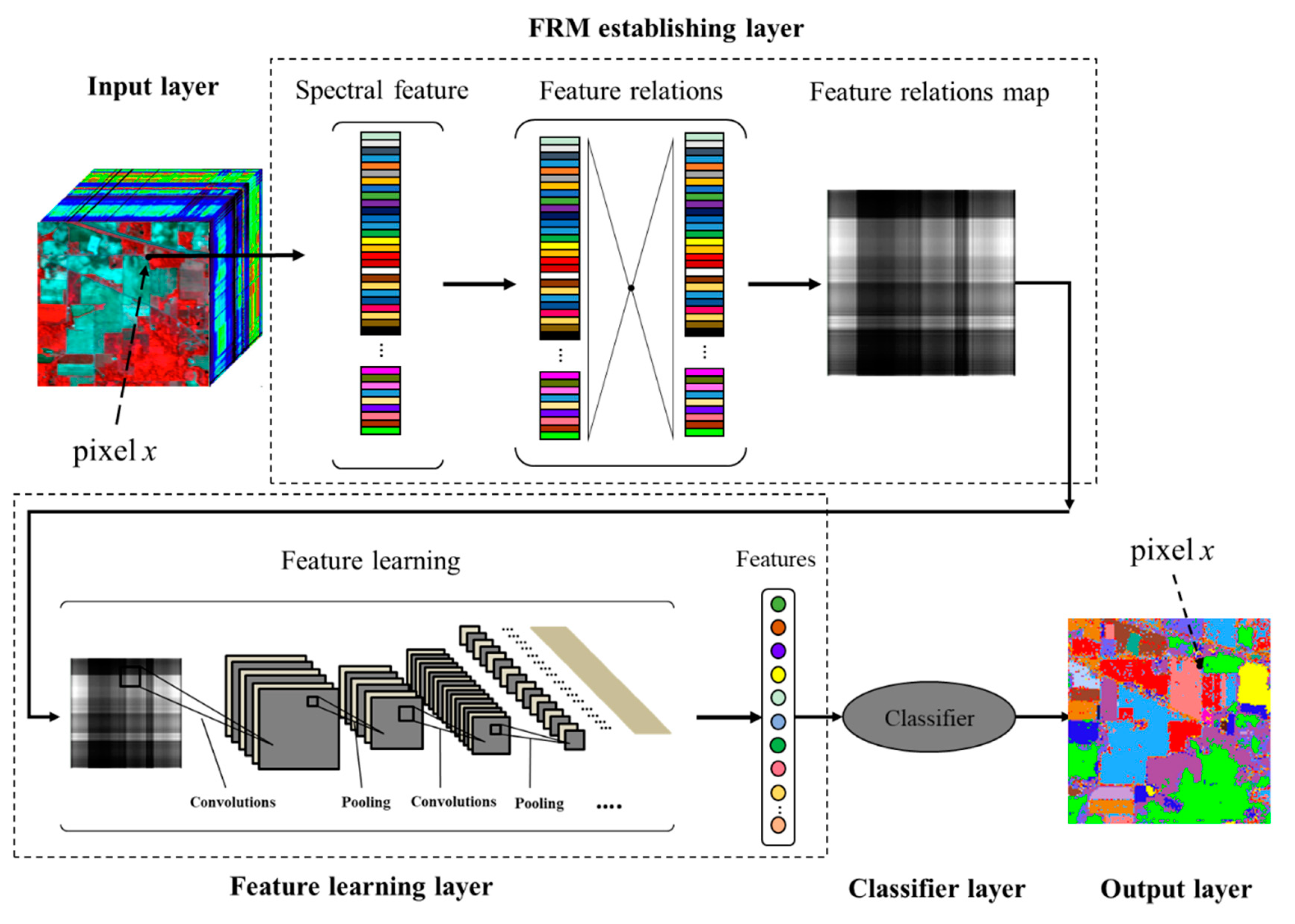
Figure 1 illustrates a hyperspectral image classification framework with the use of FRML. The framework includes an input layer, a feature relations map (FRM) establishing layer, a feature learning layer, and a classifier layer. In the first layer, each pixel in an image can be recorded as a high-dimensional vector whose entries correspond to the spectral features in each band. In the second layer, the value of each two entries can be calculated with a normalized difference index (NDI) to build a 2-D matrix—called the feature relations matrix—and then the matrix can be transformed into a picture to build FRMs that continue regular textures. In the third layer, the convolution layers of CNN can be used as a feature extractor (FE) to extract new features from the picture. In the fourth layer, the new features can be used as the input of the classifier and the final result can be predicted and signed with a class label. The classifier in the FRML can be established by any supervised classification algorithm. In this paper, we used classification and regression trees (CART) [45], random forests (RF) [46], and deep belief network (DBN) [35], respectively, to construct the classifier of FRML framework in order to compare and find the existing regulations in the FRML.
2.1.1. Feature Relations Map Establishment
With the relations of different features, classification rules can be established. However, it is relatively complex to decide how features should be selected for a hyperspectral image classification target [6,47]. To avoid this complexity, in our experiments, we neglected feature selection and had all spectral features build relations between one another.
Normalized indices, such as the normalized difference vegetation index (NDVI), the normalized difference water index (NDWI), and the normalized difference built-up index (NDBI), can generate new features by taking spectral features as input to enhance recognizability of objects [48]. To some extent, these new features can be used to reflect the interrelations between different spectral features. Thus, in this paper, we used the NDI to establish relations between different spectral features. The NDI is shown in (1):
where i = 1, 2, …, n; j = 1, 2, …, n; n is the band count of a hyperspectral image; a and b are two mutually unequal constants. When it comes to each pixel, a 2-D matrix with an n × n dimension would be calculated with the index and a and b would then be used to adjust the matrix into an asymmetric matrix. We defined a + b = 2, and a of 0.25, 0.5, and 0.75 were tested to optimize the parameters, and finally, we found that when a = 0.75, b = 1.25 FRML had the best performance. Therefore, the default values of a and b are set as 1.25 and 0.75, respectively.
With the NDI, pixels of different classes would, respectively, correspond to different feature relation matrices. To covert these matrices into pictures, FRMs of different classes would be formed. In theory, pixels belonging to the same class would have similar textures in FRMs. Thus, the process of constructing an FRM can be considered to be a process that converts a classification that uses complex spectral features into a classification that uses regular texture pictures, which offers more features for the classification target.
Obviously, the number of hyperspectral bands determines the size of an FRM—a high dimension would enlarge the data size, which would affect data processing efficiency. To reduce the potentially large size of data, a separate strategy was designed here, as shown in Figure 2. For each pixel, the spectral dimension was divided into m segments and each segment contained s features (bands). If the band count was not an integer multiple of m, then the values in the forepart continuous bands would be copied and appended on the spectrum vector to make all segments have the same band size. The feature relation matrix of each segment was calculated to obtain the m of different FRMs and then they were combined into one multi-channel picture, which is called the segmented FRM (SFRM). In comparison with the unsegmented FRM (UFRM), which uses full spectral features to build a feature relation matrix, the SFRM has a smaller picture size and its colorful textures in the RGB color space could be used to provide more discriminative information in order to distinguish a current pixel from pixels of other classes.
2.1.2. Feature Learning Method
CNN provides a powerful feature extractor, which consists of alternative convolution and pooling layers, to generalize the features towards deep and abstract representations [37]. As it is characterized by autonomous feature learning and it provides the necessary premise for more high-precision classification, the feature extractor was also previously used in this paper to learn features from the FRM. The descriptions of the convolution and pooling layers are as follows.
Convolution layers: In the FRML, a convolution layer is fed by kernels that have a two-dimensional array of weights and a bias, which scan across an image to capture different feature representations at local and global scales. The kernels provide sharable weights for different feature maps so that the features can be learned through a reduced amount of parameters and an activation function with enhanced nonlinearity operations. Mathematically, assuming X is the input cube with a size of h × w × c, where h × w is the spatial size of X and c is the number of channels, xi means ith feature map of X. Supposing that the current convolution layer had n kernels, then the jth kernel is characterized by the weight of wj and a bias of bj. The jth feature extracted by the current layer can be expressed as (2):
where * is the convolutional operator and f (•) is an activation function that is used to strengthen the nonlinear expression. ReLU is considered to be an effective activation function, which has advantages of fast convergence and robustness for gradient vanishing [7]. Thus, in this paper, we used ReLU as the activation function of the convolution layer.
Pooling layers: The pooling layers are periodically inserted after several convolution layers for down-sampling, while retaining the invariance of features to scale, offset, and shape. With the pooling operation, the parameters and feature map size are reduced for computation and the representation of the extracted feature becomes more abstract. Generally, the common pooling functions include max-pooling, average-pooling, L2-norm pooling, and weighted pooling [7,39]. In this paper, we used the most popular max-pooling function to establish pooling layers.
With the convolutional and pooling layers, we designed a three-layer convolutional network as the FRML feature extractor (the construct of the feature extractor is further illustrated in Section 3) and expected to discover FRM laws that would improve classification accuracy. In order to ensure that our experiment would be performed with high efficiency, we used TensorFlow’s Application Programming Interface (API) for programming. TensorFlow is a very famous open-source software library that was developed by the Google Brain Team for machine learning applications [48]. It provides sophisticated DL approaches, including the necessary FRML support, and is compatible with our graphics processing unit (GPU) for speeding up the operation.
2.1.3. Classification Method
Based on the features extracted from FRMs, CART, RF, and DBN, which belong to a single classifier, the EL and DL are separately used to train the FRML classifiers. CART is a decision tree-based classification algorithm that was built by dividing the sample set layer by layer, where the split property is the one that has the highest information gain ratio with the sample set and the optimal threshold under the split property obtained by information entropy calculation [45,49,50]. The RF combines the Bagging technique with the random subspace method and ensembles a set of CART classifiers to improve classification accuracy. Since it reduces the classification bias and eliminates overfitting in the decision tree construction, the RF has high accuracy and is reported to be an excellent EL method for RS image classification [12,14,51]. DBN is a popular deep learning architecture in the field of classification, consisting of several layers of restricted Boltzmann machines (RBMs) and one backpropagation neural network layer [35,52]. In DBN, RBM is an unsupervised network that consists of both visible and hidden layers. The hidden layer serves as a visible layer for the next and a pair of units from either of the two layers have a symmetric connection between them. With RBMs, probability distributions over their sets of inputs can be learned and used to train the backpropagation neural network [35]. In this paper, these classifiers were realized by using the scikit-learn library in Python.
2.2. Measurement of the Feature Relations Map Difference
FRMs are different for different classes, which can be considered to be an important basis for distinguishing between different objects. The structural similarity index measure (SSIM) is a full reference metric that is used for measuring the similarity of two images [53]. It comprehensively measures their differences through image brightness, contrast, and structure and it has advantages in terms of image difference discrimination. Hence, it can be used to judge the FRMs difference. If the SSIM of two FRMs is smaller, then there would be more difference between them, reflecting that corresponding objects are more easily distinguishable. Supposing that x is the target image and y is the reference image, then the SSIM of x and y can be defined as (3):
where μx (or μy) represents the empirical mean of x (or y), σx (or σy) is the empirical standard deviation of x (or y), σxy means the empirical correlation between x and y, and C1 and C2 are given constants.
2.3. Measurement of the Separability of Different Class Samples
For classification problems, the quality of features determines the separability of different classes. The higher the separability between different classes, the simpler the classification for ML would be. The Jeffries-Matusita distance (JMD) is a very widely used statistical separability criterion, which involves the covariance metrics of the separability measurement [54]. Since it can be used to pairwise measure the separability between classes, the JMD provides an effective assessment of the quality of different class samples in the available feature space. To evaluate the separability of samples with features learned from FRMs, the JMD between class ci and cj, which are members of a set of n classes, is defined as follows (i = 1, 2, …, n; j = 1, 2, …, n):
where bij is the Bhattacharyya distance between ci and cj; Mi and Mj represent the mean values; Ni and Nj denote the covariance matrices of classes ci and cj. Generally, the JMD is a transformation of the Bhattacharyya distance from the [0, inf] range to the fixed [0,2] range—if the JMD is closer to 2, then the separability of samples belonging to two different classes would be higher.
2.4. Accuracy Verification
Cross-validation is a primary method for estimating the skill of an ML model on a limited data sample set. In this paper, to verify the classification performance of FRML, a five-fold cross-valuation method was designed. First, the sample set was divided into five folds. Then, each fold was trained and combined with the other four folds in order to be used for testing. By training the FRML modes and verifying them, five evaluations were obtained. Finally, the highest of the five evaluation values was taken as the final verification. In our experiment, the commonly used quantitative indices, including overall accuracy (OA), kappa coefficients, and accuracy at per-class level, were used for the vivification of the hyperspectral image classification.
3. Dataset Descriptions and Experimental Designs
In our experiments, four popularly used hyperspectral image datasets, including Indiana Pines (IP), Salinas (SA), HyRANK-Loukia (HL), and Pavia University (PU) [55,56,57], were utilized to evaluate the performance of FRML.
The IP dataset was gathered using the Airborne Visible/Infrared Imaging Spectrometer (AVIRIS) sensor over the Indian Pines test site in Northwest Indiana. After removing the bands that cover the region’s water absorption, the dataset consisted of a total of 220 bands with a pixel size of 145 × 145, a spatial resolution of 20 m, and spectral coverage from 400 to 2500 nm. The SA dataset was collected by the 224-band AVIRIS sensor over the Salinas Valley in California. This dataset was characterized by a high resolution of 3.7 m. It discarded 20 water absorption bands, this including a total of 204 bands. The HL represented an image in the HyRANK dataset obtained using the Hyperion Earth Observing-1 sensor. It has a spatial resolution of 30 m and spectral coverage from 400 to 2500 nm. Following a pre-processing step, the image provided 176 surface reflectance bands with a pixel size of 249 × 945. The PU dataset was acquired through the Reflective Optics Systems Imaging Spectrometer (ROSIS) sensor during a flight campaign over Pavia in northern Italy. It constituted an image of 610 × 340 pixels, with 103 bands, spectral coverage from 430 to 860 nm, and a spatial resolution of 1.3 m.
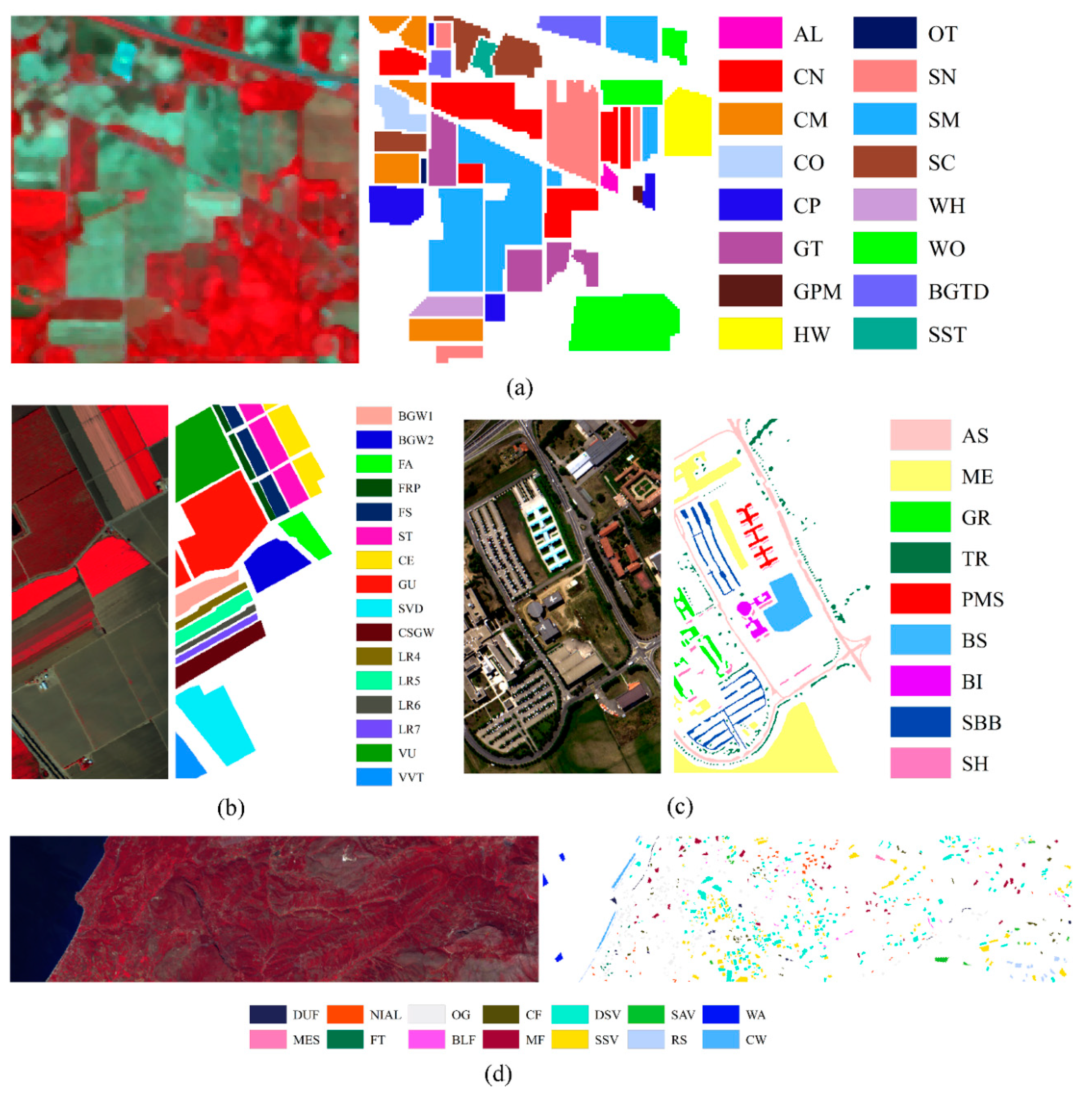
These four datasets provided high-quality benchmark information through expert visual interpretation and field investigation. The sample information of the datasets is listed in Table 1, while their false color composition pictures and corresponding ground truth maps are shown in Figure 3.
Our experiments were conducted in three parts. The first part analyzed the FRM character and the second part analyzed the samples’ separability using the features learned from SFRMs. The third part reported the classification performance of FRML and comparing methods. As the purpose of the experiments was to evaluate the feature learning results of FRML, we conducted the experiment under the same conditions. First, we set the same configuration for the feature extractor in FRML as the one shown in Table 2. Second, we used CART, RF, and DBN classifiers with the same parameters as illustrated in Table 3. All experiments were implemented using an i9-9900K 3.6 GHz processor with 32 GB RAM and the NVIDIA GeForce RTX 2080 Ti graphic card.
4. Experimental Results and Analysis
4.1. Feature Relations Map Analysis
4.1.1. Feature Relations Map Results
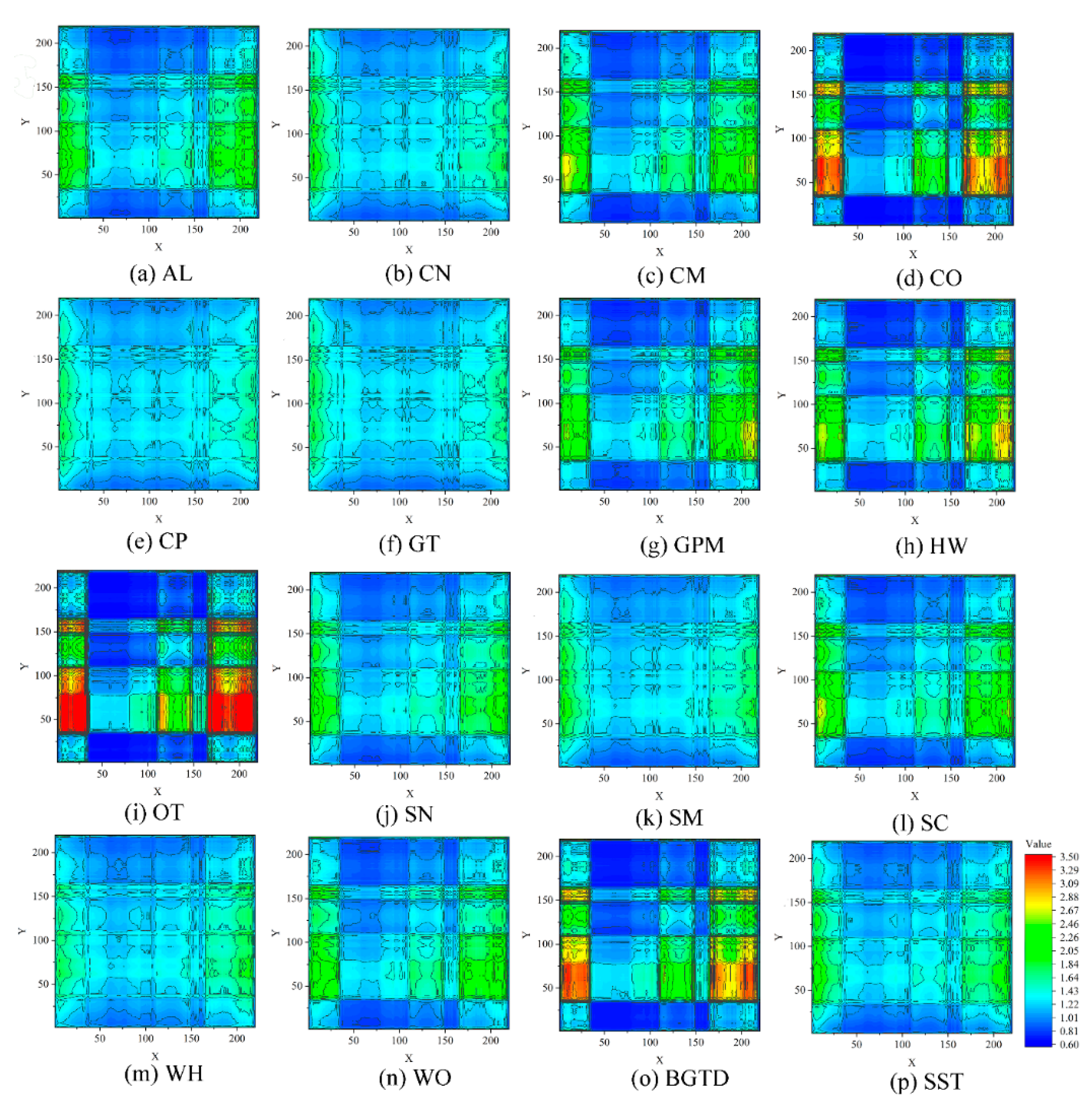
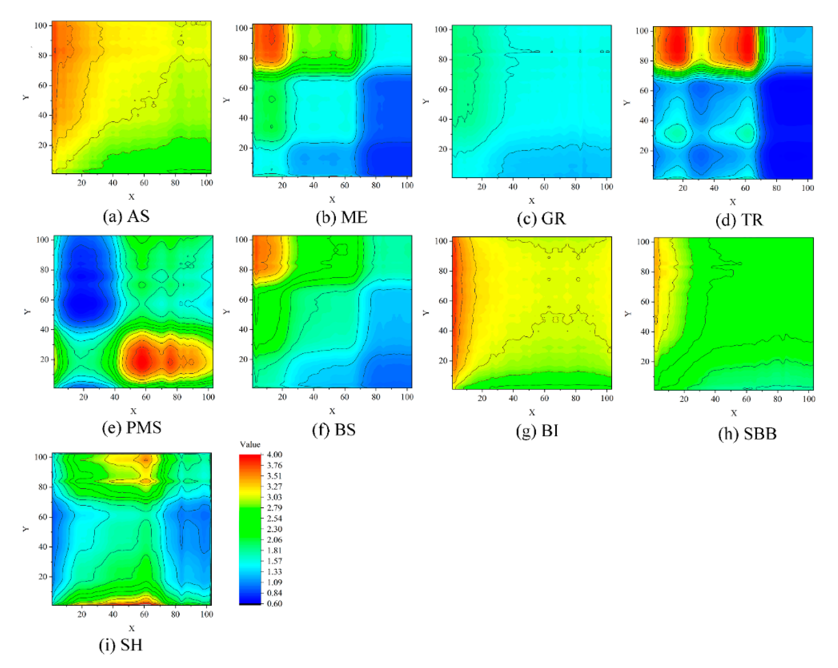
In order to explore the nature of FRM, we first established UFRMs for all samples and calculated the average value in pixels for each class in order to obtain an averaged UFRM. Due to space limitation, only the UFRMs of IP and PU datasets are shown in Figure 4 and Figure 5. Visually, these UFRMs reflect different numerical distributions. The UFRMs of the PU dataset obviously show differences between different classes with strong recognizability. In the IP dataset, some similar classes, such as SN, SM, WH, and WO, exhibit some similarities in their UFRMs, however, if the contours are carefully observed, it would be found that many differences in detail exist in them. These features indicate that, for a hyperspectral image, different classes have different FRMs, which can be used to distinguish them from others. In comparison with the spectral feature, which has only one-dimension, the FRMs provide more intuitive two-dimensional graphic information for distinguishing different patterns.
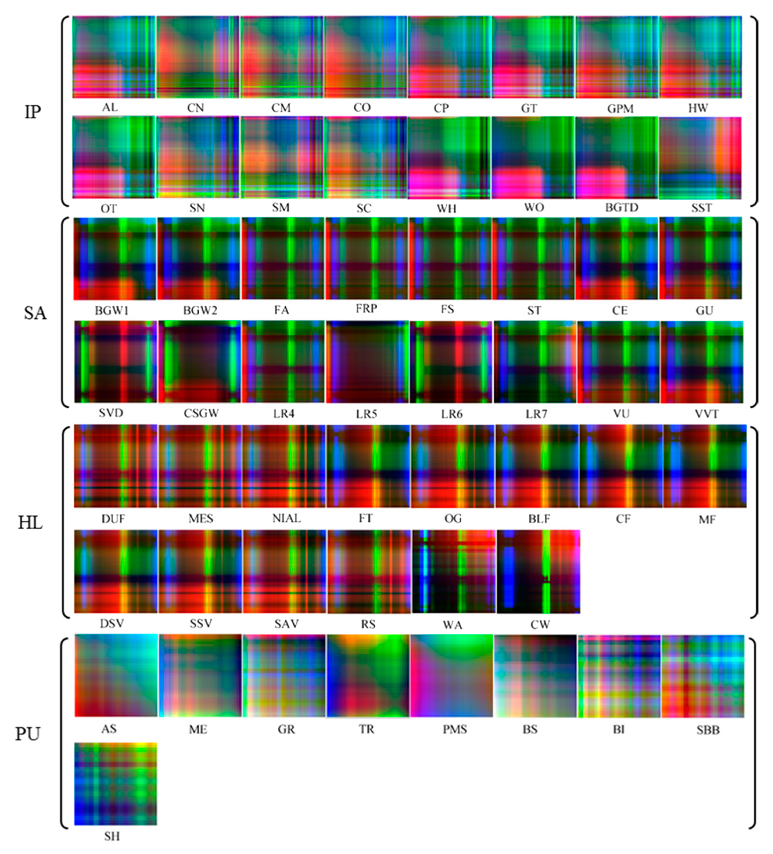
In order to reduce data size and processing time, the SFRM was designed as the final FRM of the FRML in our experiments. In these experiments, we took into consideration that the band counts of four images are different, thus the segment counts of the SFRMs for the IP, SA, HL, and PU datasets were set as 4, 4, 3, and 4, respectively. Displaying the first three channels using the RGB color form, the SFRM of each class in the four datasets is shown in Figure 6. The SFRMs of different classes exhibit different texture patterns (this feature is very obvious in the IP and PU datasets). Although some SFRMs have similar textures visually, they still have differences in brightness and color. This means that, using the segmented strategy, the SFRMs have the same capability as the USFRMs to distinguish between objects of different classes.
4.1.2. Feature Relations Map Differences
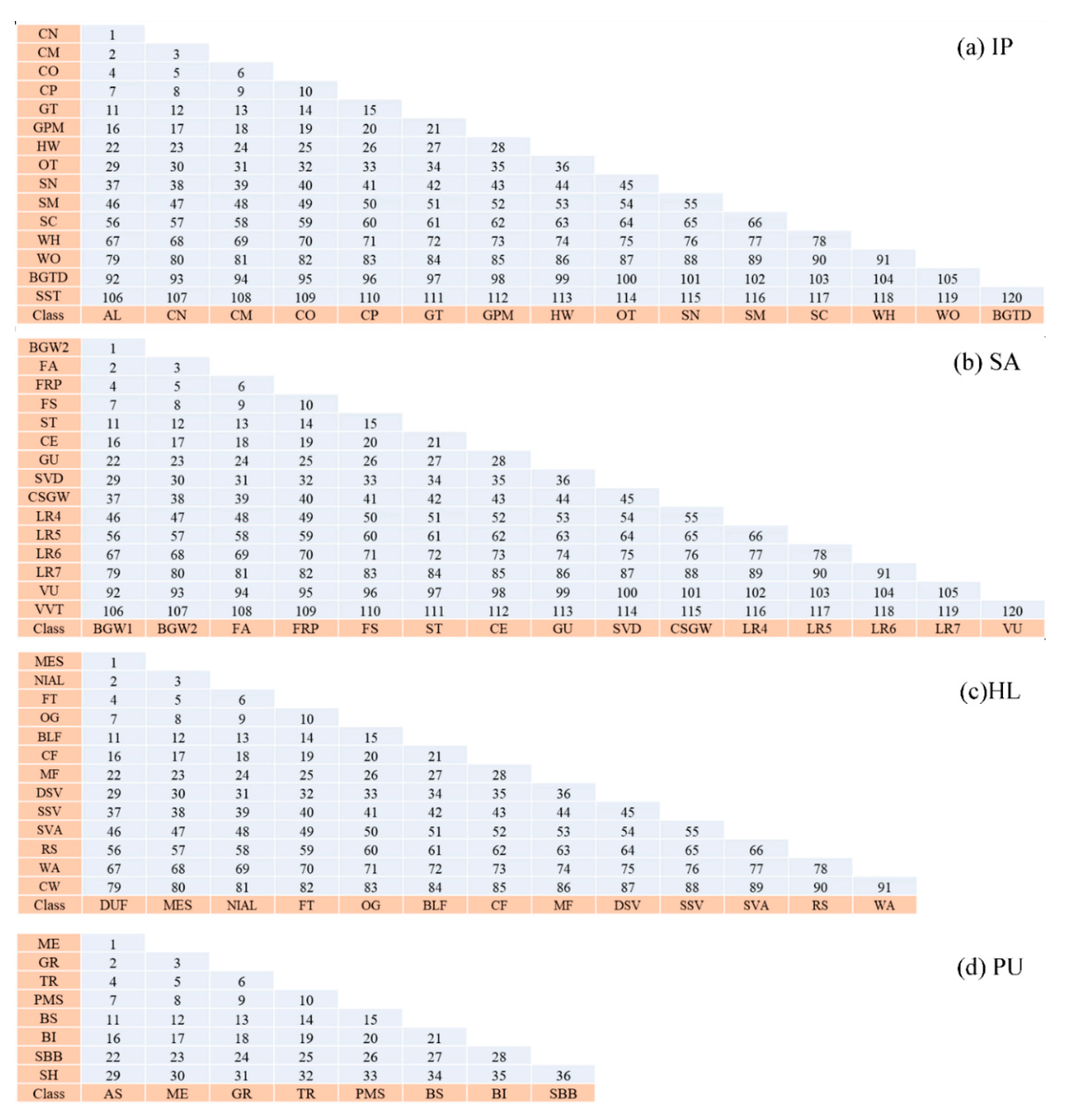
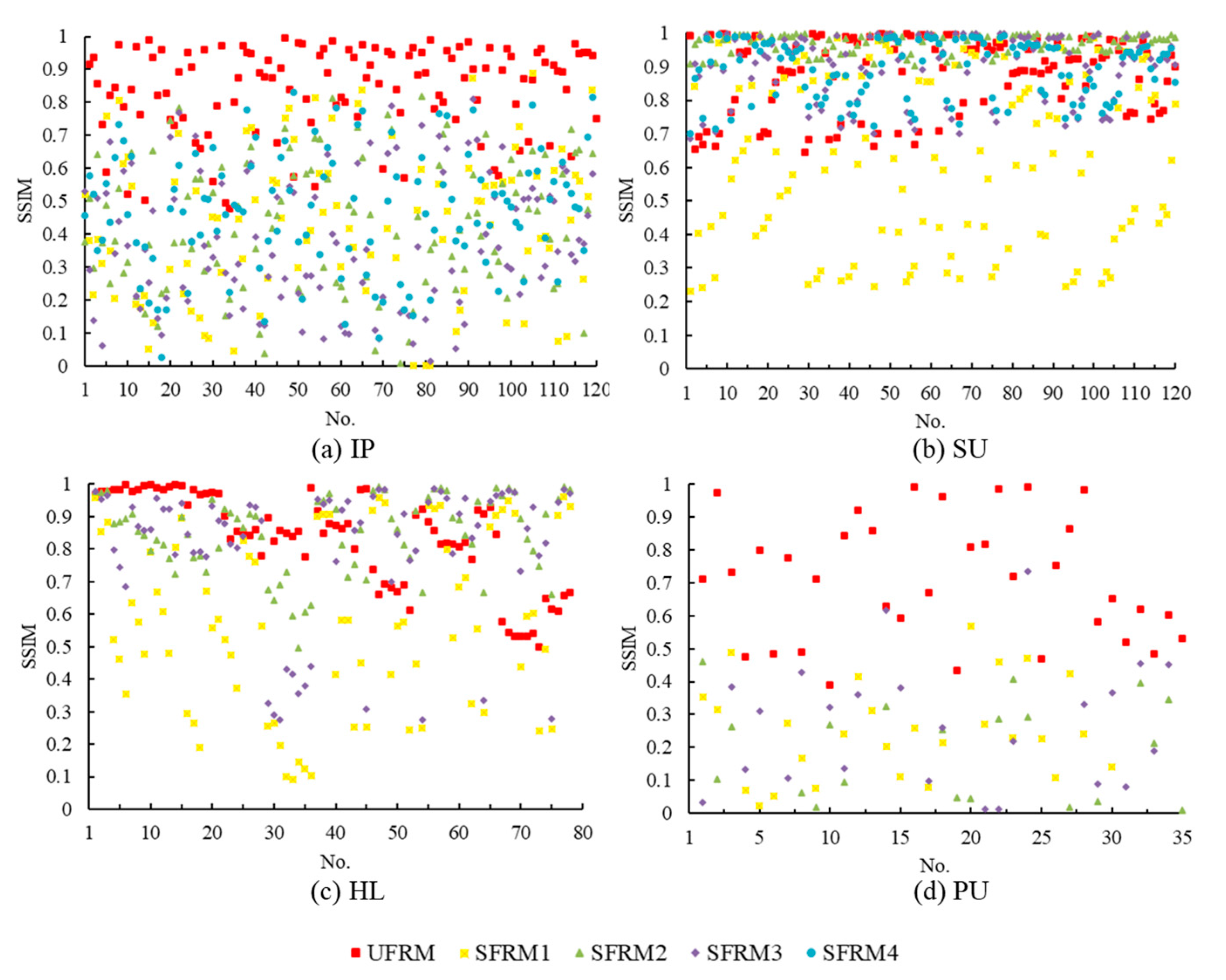
The differences between FRMs made samples of different classes separable. To evaluate these differences, the SSIM was calculated in the experiment. For a convenient description of the SSIMs between different classes, each pair of classes was numbered to obtain an index, as shown in Figure 7. Then, according to the indices, the SSIMs of SFRMs (or UFRMs) for each pair of classes were illustrated as scatter plots shown in Figure 8. Clearly, it can be observed that, for some classes, there is a great difference between their UFRMs with low SSIMs but that, for some other classes, the SSIMs are higher than 0.9, exhibiting great similarities that increase the difficulty to distinguish between objects using the UFRMs. This may be because, when the NDI was used to establish feature relations, some highly related spectral features interacted with one another, resulting in some very similar results that could not reflect differences very well. SFRMs establish relations between features in an interval of the hyperspectral spectrum. In comparison with the UFRMs, some channels of SFRMs exhibit lower SSIMs, reflecting more significant differences between different classes. This channels make great contribution to the SFRM, and with the SFRM, the objects of different classes would be more separable. When the segmentation strategy is used, the interaction of the highly relevant features is reduced, resulting in SFRM discriminations for different classes being heavily improved. This shows that SFRM could provide a favorable basis for the classification using the relations of different spectral features.
4.2. Sample Separability with Features Learned from SFRMs
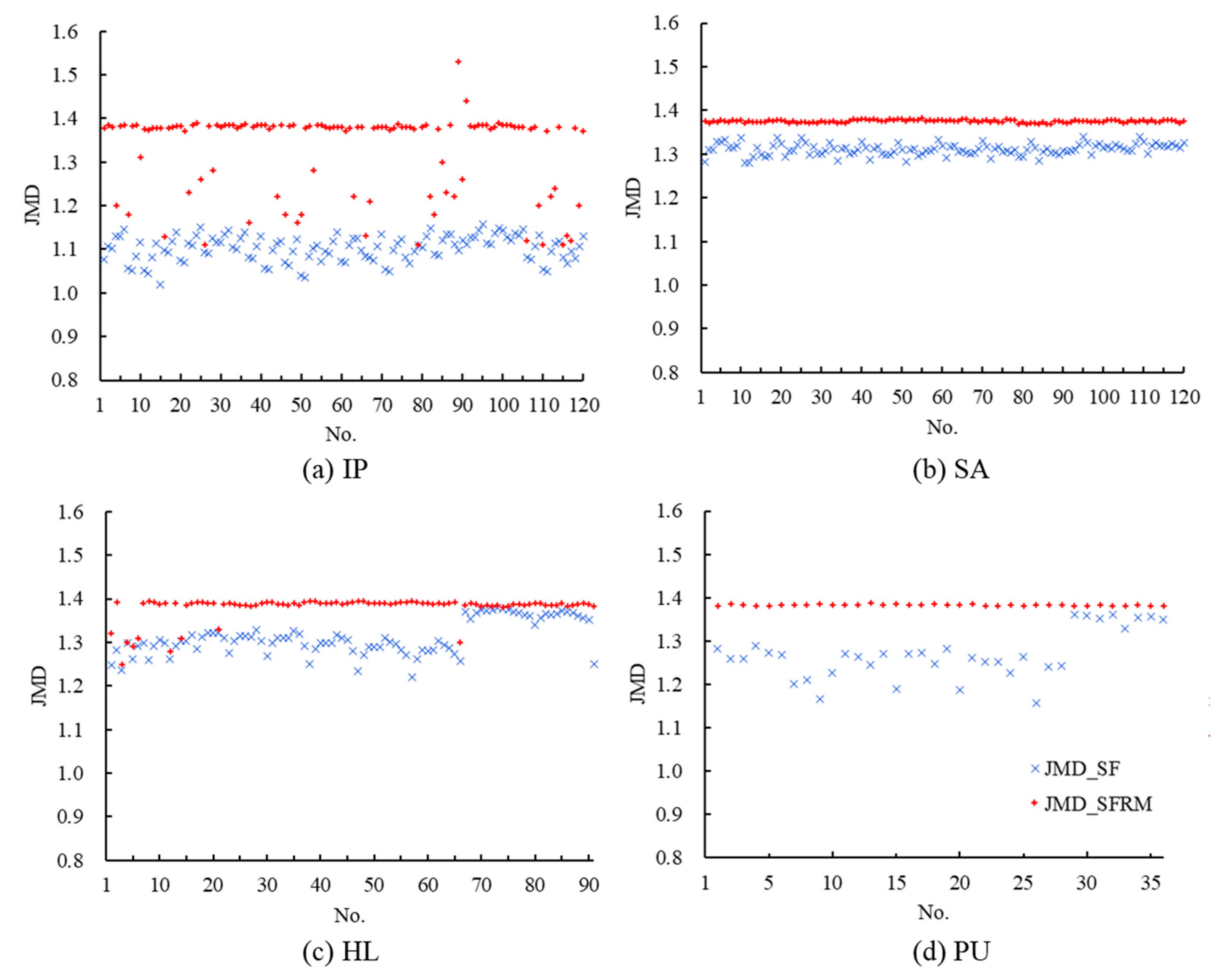
In our experiment, SFRM features were learned using the feature extractor and the separability of samples for a pair of classes was evaluated using the JMD. As shown in Figure 9, for the four datasets, the JMDs are higher under the features that learned from SFRM (JMD_SFRM) than the JMDs under the spectral features (JMD_SF), reflecting strong separability of each pair of classes. For example, for the IP dataset, the JMD_SF of each pair of classes is located in 1–1.2, while the JMD_SFRMs are basically greater than 1.38, indicating that the features learned from the SFRMs are more discriminative than the original spectral features. All these dataset cases indicate that SFRM provides two-dimensional material, such as textures and graphics, which can be used to learn more discriminative features with the deep convolutional network. Through feature learning, the SFRM differences are transformed into high-quality features, which would be more convenient for the classification of different objects because of their higher separability.
4.3. Classification Results and Analysis
In this section, the features learned by FRML and those learned by other methods of comparison are evaluated. As we focus more on the capability of feature learning, only the feature extractor of the comparative methods, including the recently proposed long short-term memory (LSTM), multiscale CNN (MCNN), spectral-spatial unified networks (SSUN), random patches network (RPNet), three-dimensional scattering wavelet transform (3DSWT), and extended random walkers (ERW), were used in our experiments. For the LSTM, MCNN, and SSUN, the parameters were set to the default values given in [55]. For the RPNet, 3DSWT, and ERW, the parameters were set to the default values given in [57,58]. With the features learned by FRML and the comparative methods, the classification stage was conducted using the CART, FR, and DBN classifiers, respectively, and the final classification accuracies are shown in Table 4.
4.3.1. Classification Performance at the Overall Level
As reported in many research studies, CART is a weak classifier in comparison with strong classifiers such as SVM and AdaBoost. In our experiments, CART was first used to evaluate classification performance with features extracted using different methods. It was found that, with using the CART classifier, some feature extract methods exhibit low accuracy. For instance, the CART-based LSTM had an OA of only 73.85% (kappa = 0.703) in the test on the IP dataset, while the CART-based SSUN achieved an OA of 75.33% (kappa = 0.780) in the test on HL dataset. This feature indicates that, when features are extracted by some comparative methods, CART does not seem to be an optimal classifier. The phenomenon may be caused by two reasons—that CART performance is weak or that features extracted by comparative methods are not discriminative enough for classification using CART. However, when it comes to the FRML, the CART-based FRML achieved very satisfying classification results with an OA higher than 96%. For the IP, HL, and PU datasets, the CART-based FRML achieved the highest accuracy compared to any of the other CART-based methods. The CART-based FRML for the SA dataset had an OA of 98.19% (kappa = 0.980), which was 1.3% lower than that of the CART-based ERW which had the highest accuracy. Under the same parameter conditions, the reason why the CART-based FRML had higher accuracy is because FRML had learned more discriminative features than comparative methods, resulting in pixels that are more separable in the classification.
In comparison with CART, RF had a higher accuracy in our evaluation. In the HL and PU datasets, the RF-based FRML achieved the highest OAs of 98.48% and 98.97%, respectively. In the IP dataset, the RF-based FRML had a higher accuracy than most of the comparative methods in its group, except for the RF-based MCNN, while in the SA dataset, the accuracy of the RF-based FRML was lower than the RF-based MCNN and the RF-based ERW, although the differences were very small—differing only by 0.45% and 0.93%, respectively. These results indicate that, with a strong classifier like RF, FRML could achieve more accurate classification. Expecting the comparative methods whose accuracy also obviously improved due to RF, the classification accuracy improvements of some other comparative methods are not as good as those of FRML. This phenomenon may be due to the fact that current methods are not suitable for classification with the RF classifier; however, another possible explanation is that the features extracted by these methods do not discriminate as well as FRML does.
In the group in which DBN was used as an evaluating classifier, FRML had the highest classification accuracy on all datasets, except for the IP dataset—where the DBN-based FRML had an OA of 96.29%, lower than the DBN-based ERW and the DBN-based RPNet and very close to that of the CART-based FRML. In comparison with other feature extract methods, using DBN as a classifier obviously improves classification accuracy more than using CART—however, the performance of the DBN-based FRML on the IP dataset indicates the opposite. This phenomenon may be due to the fact that fixed DBN parameters set in our experiments were not optimal for the IP dataset. Another reason may be that there was an imbalance in the training set, where some classes, such as GPM and OP, were underrepresented due to too few samples.
Taken together, in most cases, FRML outperforms the comparative methods in the four datasets. To evaluate the robustness for each method, the average accuracy of the four datasets was calculated as shown in Table 4. From the results, it can be seen that the CART-based and RF-based FRMLs had the highest average accuracy in comparison with the other methods in their groups. The DBN-based FRML exhibited almost the same average accuracy as the DBN-based ERW, which was higher than that of the other methods. This phenomenon suggests that the FRML methods are more robust than the comparative methods.
FRMLs exhibit stable performance in different datasets under the sample parameter conditions, with strong generalization and easier operation. This may be because FRMLs obtain optical features to improve the separability of the pixels in classification. Last but not least, FRMLs learn features from the relations of spectral features and, in comparison to other feature extraction methods, FRMLs make full use of the different bands of hyperspectral images, providing more abundant information with a higher quality for classification accuracy improvement.
4.3.2. Classification Performance at the Per-Class Level
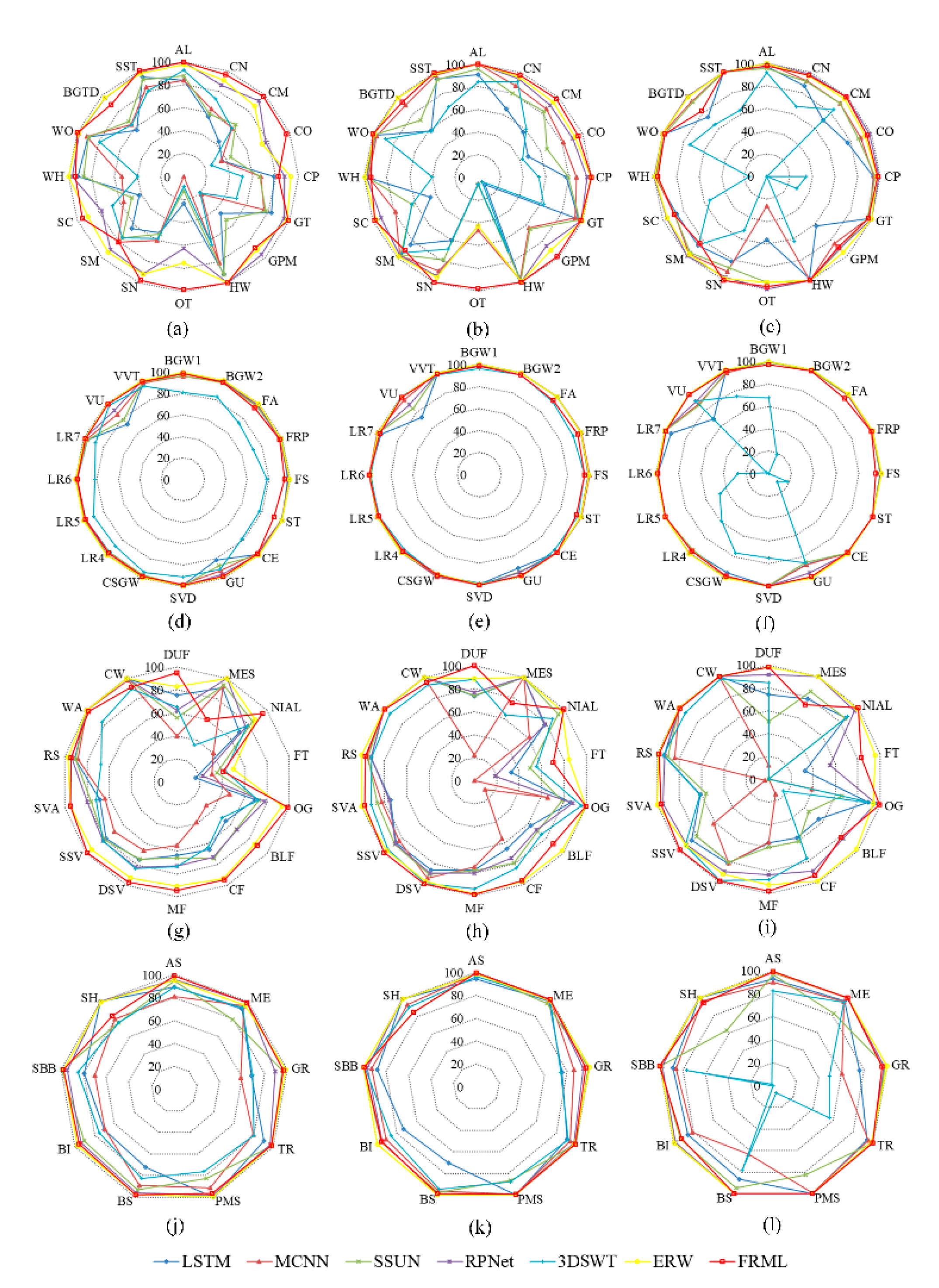
To explore the FRML hyperspectral image classification ability, the classification accuracy at the per-class level is reported and illustrated in Figure 10. For the IP dataset, most classes achieved a higher accuracy with FRMLs than with comparative methods. Especially for the OT, the accuracy was not very good when comparative methods were used, while it obviously improved with FRML. For the SA dataset, the VU and GU do not seem to be satisfactorily classified with a high accuracy using the features extracted through comparative methods, except for ERW—when the accuracy reaches a very higher level while using FRML. FRML maintains a higher classification accuracy in the HL dataset for most individual classes, except for EMS, in comparison with most other methods. For the PU dataset, FRML also exhibits excellent performance for most individual class classifications compared to comparative methods. These features suggest a good improvement at the per-class level using FRML. In comparison with other methods, only few individual classes were not improved to the highest level, perhaps because the FRMs of these classes were too similar to those of other classes and their features—extracted by the CNN-based feature extractor designed in our experiments—were not discriminative enough yet. However, FRML did exhibit a better balance of accuracy improvement for all classes than comparative methods and this phenomenon is especially obvious in the IP and HL datasets. Clearly, FRML improves hyperspectral image classification not only at the overall level but also at the per-class level. As SFRMs provide good separability between different classes in FRML (as shown in Figure 5 and Figure 8), they greatly reduce potential misclassifications for each class.
4.3.3. Impact of the Training Sample Size on FRML
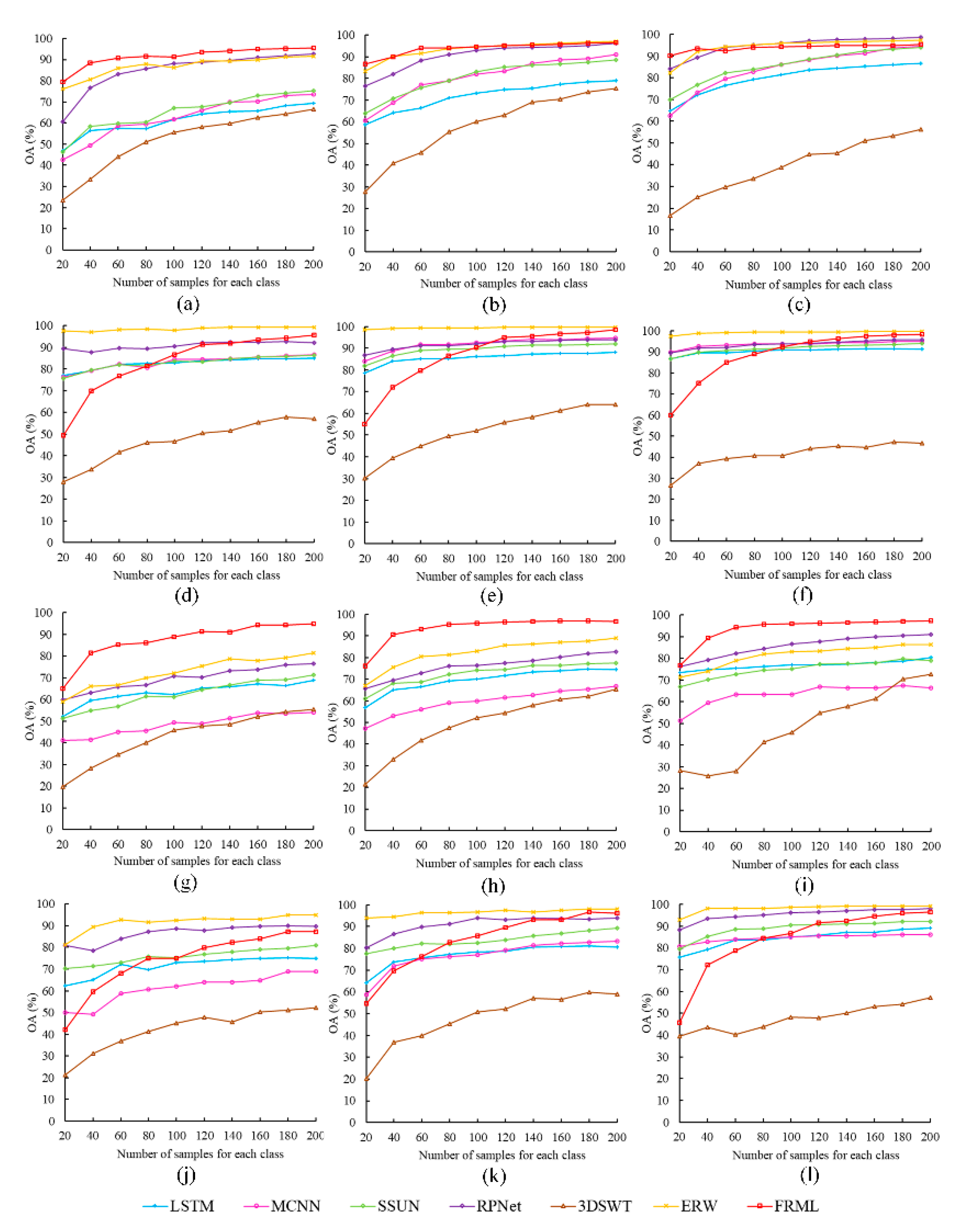
The impact of sample size for RS image classification has been reported in many research studies [7,32,39]. Grasping the influence of sample size on the accuracy of a classifier can effectively guide RS image interpretation. To evaluate how the sample size impacts FRML classification accuracy, 200 samples for each class were randomly selected from the training set to produce a new sample set. Then, classifiers were trained with the samples, whose size gradually increased by 10% of the sample set size, and the classification accuracy was evaluated by testing a set that contained samples that were not selected. The OA changes in FRML and other comparative methods are shown in Figure 11. With the increase of training sample set size, the CART- and RF-based FRMLs on the IP and HL datasets exhibited excellent accuracy improvement performance, beating all other comparative methods. This feature suggests that FRML has the potential to achieve higher-level accuracy with a limited sample size. However, it is difficult to ensure that FRML can obtain higher accuracy than all comparative methods because the characteristics of the datasets used are different. For the PU and SA datasets, the ERW method had a higher accuracy than FRML, the FRML method seemed to require a larger number of training samples to achieve an accuracy that would be equal to or similar to the accuracy achieved by ERW. This phenomenon, on the two datasets, reflects a stronger dependence of FRML on the number of training samples than that of other methods for improving classification accuracy and it is also worth noting that, with the number of training samples increasing, the increases in the accuracy of FRML are larger than for most of the comparative methods. The obviously increasing FRML trends make it reasonable to conclude that if the number of the training samples is continually increasing, then there would be an even further FRML accuracy improvement.
Besides the differences between the datasets, the FRML classifier would be another important factor affecting the accuracy improvement as the number of training samples increases because, as Figure 11 illustrates, with the same number of training samples, the RF-based FRMLs have better accuracy improvement than the CART-based FRMLs. In the PU dataset, especially, the CART-based FRML seems to need more samples to improve accuracy to a higher level than the RF- and DBN-based FRMLs. Thus, if more accurate classification with a smaller sample size is desired, then the appropriate FRML classifiers should seriously be considered.
4.3.4. Land Use Mapping with FRML
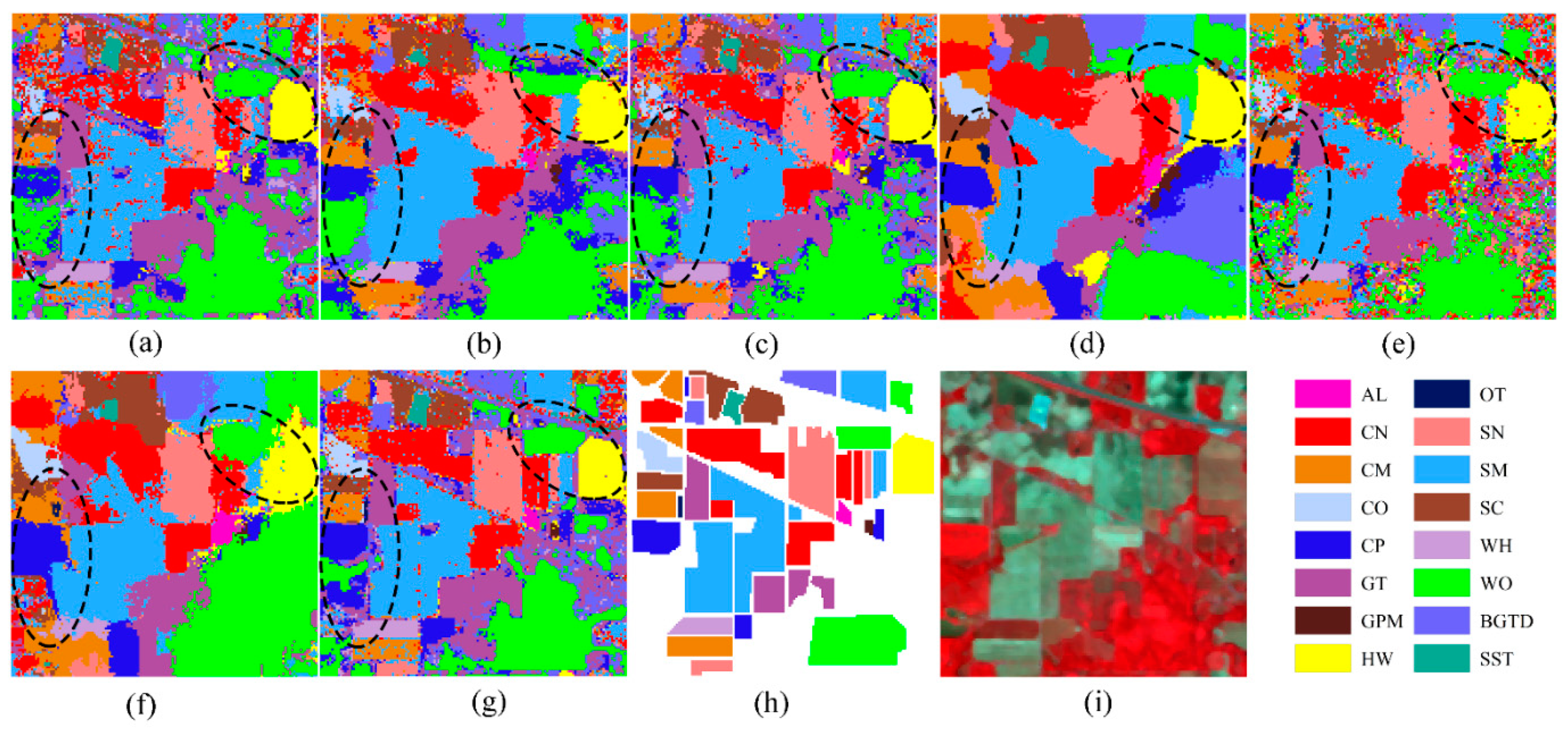
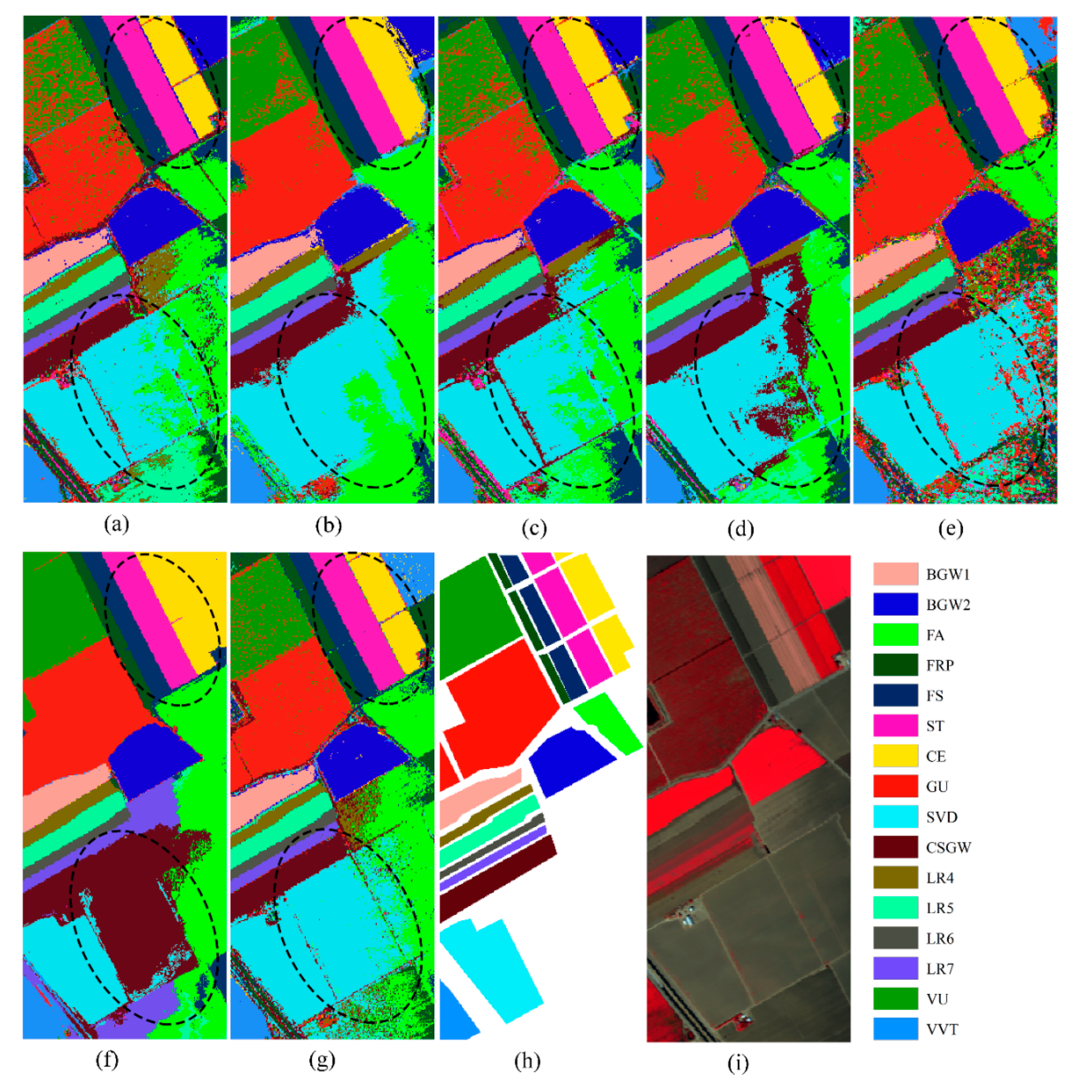
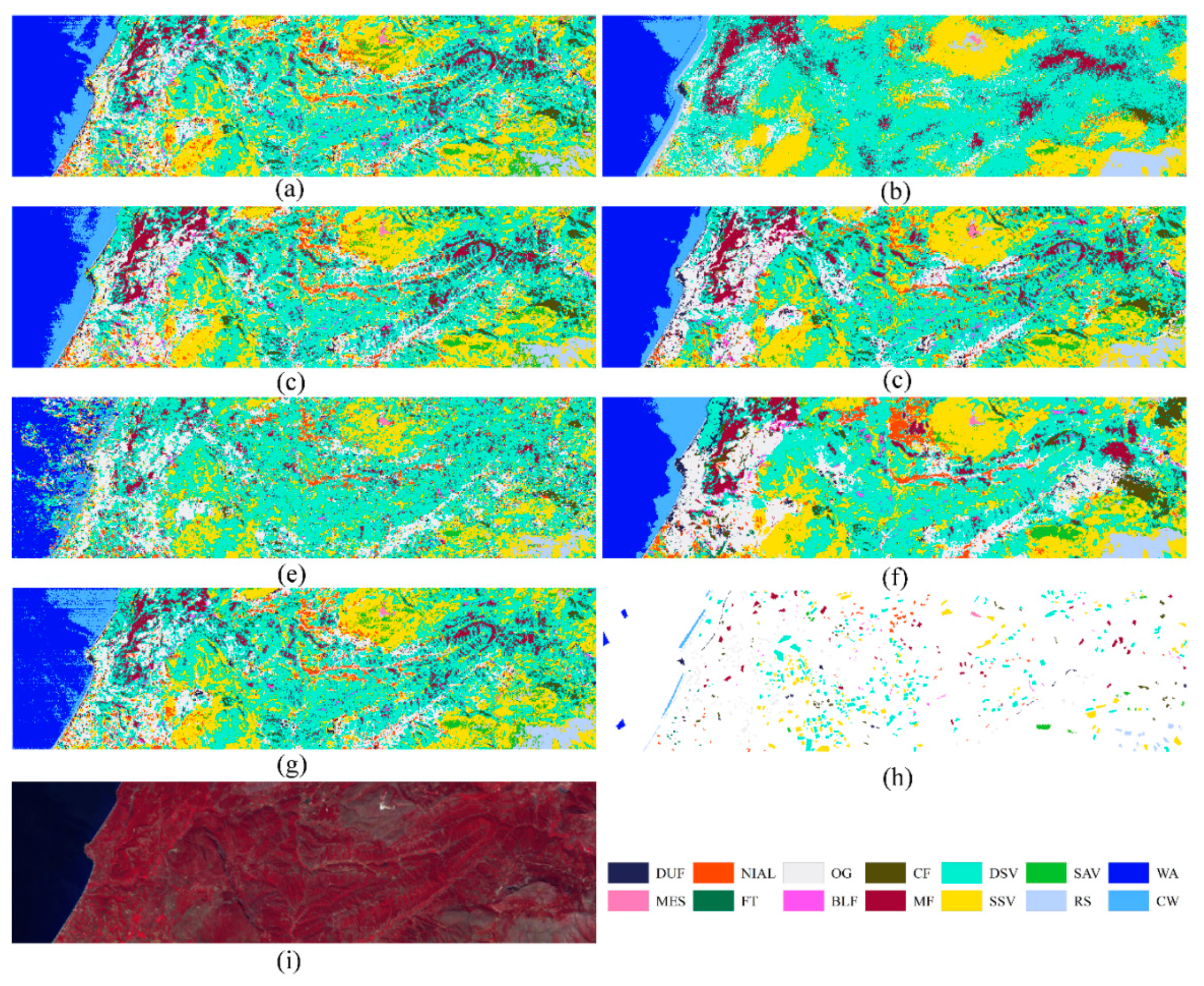
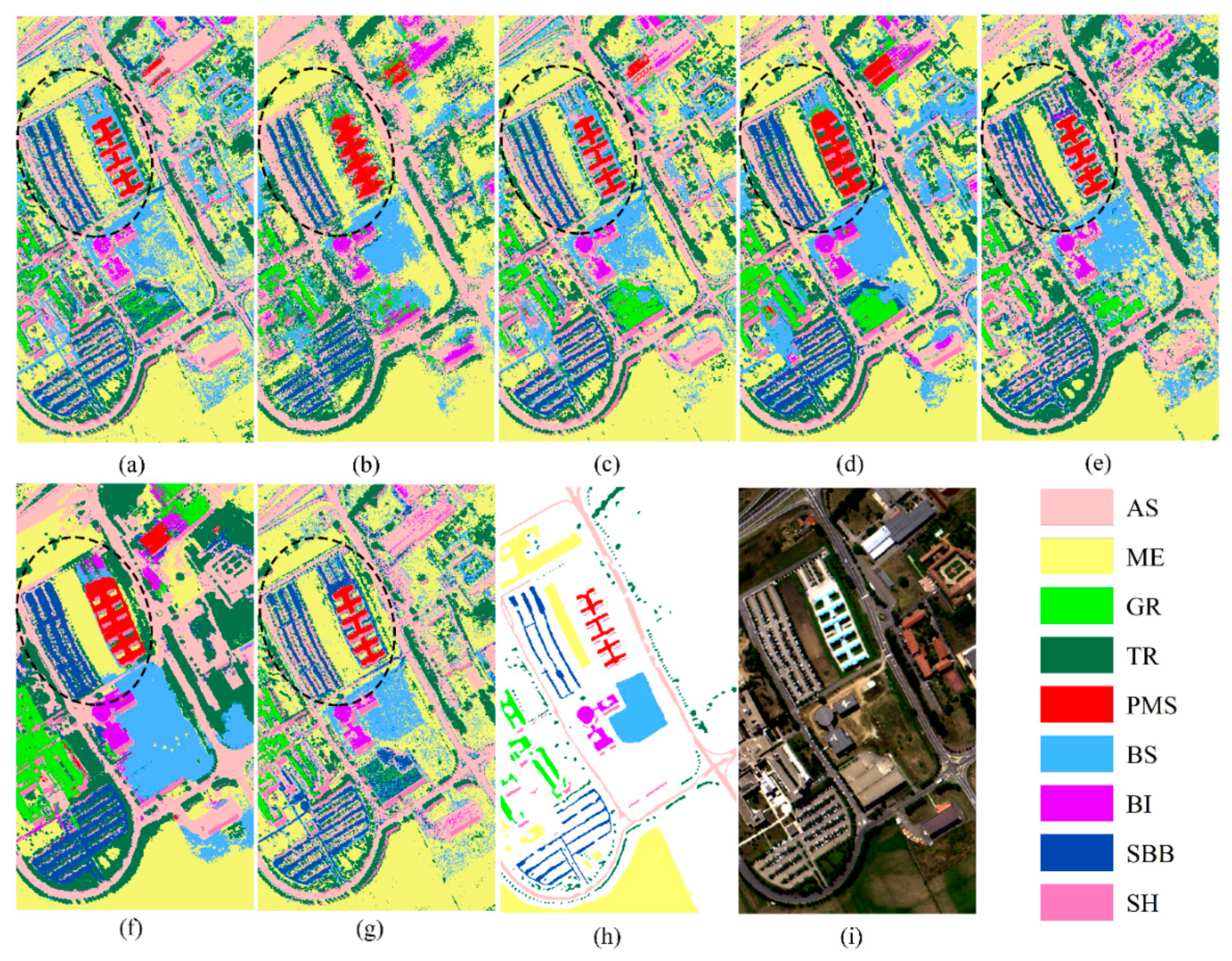
To estimate the FRML property for land use mapping, the four datasets were classified using different methods. Due to limited space, we only showed the maps that were classified by RF (as shown in Figure 12, Figure 13, Figure 14 and Figure 15). In the maps for the IP dataset (Figure 12), the comparative methods show obvious misclassifications between CO and WO in the left region of interest (ROI); however, with the RF-based FRML (Figure 12g), the two classes are correctly classified. The FR-based SSUN, RPNet, 3DSWT, and ERW (Figure 12c–f, respectively) exhibit fuzzy boundaries between HW and WO in the right ROI; however, with the RF-based FRML, the edge of these classes is more clear and similar to the ground truth. For the SA dataset (Figure 13), the comparative methods exhibit unsatisfactory performance when distinguishing between the SVD and FA in the button ROI; however, with the RF-based FRML, the two land use types were basically classified correctly. The RF-based FRML also has good performance in land use mapping in the HL dataset. When comparing the RF-based MCNN, 3DSWT and RF-based ERW (Figure 14b,e,f, respectively), the RF-based FRML seems to be better at describing details. For the PU dataset (Figure 15), SBB near to the PMS in the ROI were wrongly classified as BS by the comparative methods, while the SBB were correctly classified using the RF-based FRML.
In the evaluation of classification accuracy, the RF-based MCNN in the IP dataset, as well as the RF-based RPNet and ERW in the SA and PU datasets, have a very high accuracy of more than 98%—even higher than the FR-based FRML. However, in the mapping experiments, the maps of these datasets exhibit some fuzzy and distorted boundaries between different objects (as shown in Figure 12b, Figure 14d,f, and Figure 15d,f), while some details were also erased. This phenomenon may be caused by the spatial fitters that these methods use to smooth the features of boundaries and details. With FRML, the features of each pixel have no spatial information obtained by filters—thus, it could maintain more land use details on the map. However, as adjacent pixels are independent and without special information, the maps produced by FRMLs would be affected by the salt and pepper noise in the images.
4.3.5. Time Cost
Table 5 lists the time consumption of feature extraction with different methods. For FRML, the time was mainly consumed by SFRM establishing and feature learning. Obviously, SFRM establishing (SFRM-E) is a first-time consumer in FRML, which may be due to multiple loops used for feature relation value calculation in the procedure code. Feature learning from SFRM (FL-SFRM) seemed to consume less time than SFRM-E. For the four datasets, the FL-SFRM spent 2.41–6.21% of the time used for SFRM-E. In comparison with the other methods, FRML took more time to extract features in most cases in our experiments. This time cost of the feature extraction methods could be affected by the codding and computing platform, but it could also be concluded that FRML is a time-consuming algorithm due to SFRM-E; thus, accuracy should be the most important factor in performance evaluation.
5. Conclusions
By establishing relations between different spectral features using NDIs, it was found that each class has its own FRM that could be used to distinguish it from other classes. FRMs not only generate new features but also provide two-dimensional graphic information, such as textures and polygons, updating pattern recognition through using one-dimensional spectral features to regular texture pictures. Based on these findings, we proposed an FRML with SFRM (an FRM designed using a segment strategy) to classify hyperspectral images. Benefits of SFRM are that FRML could automatically enhance the separability of different objects and that it could learn more discriminative features using a feature extractor that consists of a deep convolutional network. Due to its powerful feature learning ability, FRML could archive higher accuracy than comparative methods in most cases. Unlike other feature learning methods, FRML learns features from their relationships rather than directly from the spectral or spatial features themselves—which gives FRML more chance to consider the full use of original features, without any data dimensional reduction, to obtain more objective features for improved classification accuracy and to have a stronger capability of maintaining details in mapping.
FRML exhibits excellent performance in hyperspectral image classification. However, some of its aspects still need to be improved. For example, in our experiments, only three classifiers were utilized in FRML—in order to fully explore FRML with high accuracy, more classifiers should be used to obtain the optimal FRML framework. In addition, the establishment of FRM plays an important role in FRML, however, in this paper, only DNI was used to do so. For describing the relations between different features better, more advanced methods should be explored. Last but not least, FRML suffers from a disadvantage of being time consuming; thus, the procedure code needs more optimization in order to accelerate operation speed in future studies.
To summarize, FRML successfully uses feature relations to improve hyperspectral image classification. The framework is flexible and advanced, and it is expected to be suitable for more complex RS image classifications.
Author Contributions
Conceptualization, P.D. and C.Z.; methodology, P.D.; validation, P.D. and C.Z.; formal analysis, P.D. and C.Z.; resources, P.D.; data curation, P.D.; writing—original draft preparation, P.D.; writing—review and editing, P.D. and C.Z.; project administration, P.D. and C.Z.; funding acquisition, P.D. and C.Z. All authors have read and agreed to the published version of the manuscript.
Funding
This research was funded by National Key Research and Development Program of China under grant 2018YFA0605500; China Postdoctoral Science Foundation under grant 2019TQ0233 and 2019M662698.
Acknowledgments
We would like acknowledge China National Postdoctoral Council (CNPC) for providing funding for this research.
Conflicts of Interest
The authors declare no conflict of interest. The funders had no role in the design of the study; in the collection, analyses, or interpretation of data; in the writing of the manuscript, or in the decision to publish the results.
References
- Mou, L.; Ghamisi, P.; Zhu, X.X. Deep Recurrent Neural Networks for Hyperspectral Image Classification. IEEE Trans. Geosci. Remote. Sens. 2017, 55, 3639–3655. [Google Scholar] [CrossRef] [Green Version]
- Kong, F.; Wen, K.; Li, Y. Regularized Multiple Sparse Bayesian Learning for Hyperspectral Target Detection. J. Geovis. Spat. Anal. 2019, 3. [Google Scholar] [CrossRef]
- Bansod, B.; Singh, R.; Thakur, R. Analysis of water quality parameters by hyperspectral imaging in Ganges River. Spat. Inf. Res. 2018, 26, 203–211. [Google Scholar] [CrossRef]
- Caballero, D.; Calvini, R.; Amigo, J.M. Hyperspectral imaging in crop fields: Precision agriculture. In Design and Optimization in Organic Synthesis; Elsevier BV: Amsterdam, The Netherlands, 2020; Volume 32, pp. 453–473. [Google Scholar]
- Yokoya, N.; Chan, J.C.-W.; Segl, K. Potential of Resolution-Enhanced Hyperspectral Data for Mineral Mapping Using Simulated EnMAP and Sentinel-2 Images. Remote. Sens. 2016, 8, 172. [Google Scholar] [CrossRef] [Green Version]
- Audebert, N.; Le Saux, B.; Lefèvre, S. Deep Learning for Classification of Hyperspectral Data: A Comparative Review. IEEE Geosci. Remote. Sens. Mag. 2019, 7, 159–173. [Google Scholar] [CrossRef] [Green Version]
- Li, S.; Song, W.; Fang, L.; Chen, Y.; Ghamisi, P.; Benediktsson, J.A. Deep Learning for Hyperspectral Image Classification: An Overview. IEEE Trans. Geosci. Remote. Sens. 2019, 57, 6690–6709. [Google Scholar] [CrossRef] [Green Version]
- Xia, J.; Yokoya, N.; Iwasaki, A. Hyperspectral Image Classification with Canonical Correlation Forests. IEEE Trans. Geosci. Remote. Sens. 2016, 55, 421–431. [Google Scholar] [CrossRef]
- Yang, D.; Bao, W. Group Lasso-Based Band Selection for Hyperspectral Image Classification. IEEE Geosci. Remote. Sens. Lett. 2017, 14, 2438–2442. [Google Scholar] [CrossRef]
- Khan, M.J.; Khan, H.S.; Yousaf, A.; Khurshid, K.; Abbas, A. Modern Trends in Hyperspectral Image Analysis: A Review. IEEE Access 2018, 6, 14118–14129. [Google Scholar] [CrossRef]
- Du, P.; Bai, X.; Tan, K.; Xue, Z.; Samat, A.; Xia, J.; Li, E.; Su, H.; Liu, W. Advances of Four Machine Learning Methods for Spatial Data Handling: A Review. J. Geovis. Spat. Anal. 2020, 4, 1–25. [Google Scholar] [CrossRef]
- Chan, J.C.-W.; Paelinckx, D. Evaluation of Random Forest and Adaboost tree-based ensemble classification and spectral band selection for ecotope mapping using airborne hyperspectral imagery. Remote. Sens. Environ. 2008, 112, 2999–3011. [Google Scholar] [CrossRef]
- Cao, X.; Wen, L.; Ge, Y.; Zhao, J.; Jiao, L. Rotation-Based Deep Forest for Hyperspectral Imagery Classification. IEEE Geosci. Remote. Sens. Lett. 2019, 16, 1105–1109. [Google Scholar] [CrossRef]
- Zhang, Y.; Cao, G.; Li, X.; Wang, B. Cascaded Random Forest for Hyperspectral Image Classification. IEEE J. Sel. Top. Appl. Earth Obs. Remote. Sens. 2018, 11, 1082–1094. [Google Scholar] [CrossRef]
- Ergul, U.; Bilgin, G. HCKBoost: Hybridized composite kernel boosting with extreme learning machines for hyperspectral image classification. Neurocomputing 2019, 334, 100–113. [Google Scholar] [CrossRef]
- Su, H.; Yu, Y.; Du, Q.; Du, P. Ensemble Learning for Hyperspectral Image Classification Using Tangent Collaborative Representation. IEEE Trans. Geosci. Remote. Sens. 2020, 58, 3778–3790. [Google Scholar] [CrossRef]
- Datta, A.; Ghosh, S.; Ghosh, A. Unsupervised band extraction for hyperspectral images using clustering and kernel principal component analysis. Int. J. Remote. Sens. 2017, 38, 850–873. [Google Scholar] [CrossRef]
- Jia, S.; Deng, X.; Zhu, J.; Xu, M.; Zhou, J.; Jia, X. Collaborative Representation-Based Multiscale Superpixel Fusion for Hyperspectral Image Classification. IEEE Trans. Geosci. Remote. Sens. 2019, 57, 7770–7784. [Google Scholar] [CrossRef]
- Mahdianpari, M.; Salehi, B.; Mohammadimanesh, F.; Brisco, B.; Mahdavi, S.; Amani, M.; Granger, J.E. Fisher Linear Discriminant Analysis of coherency matrix for wetland classification using PolSAR imagery. Remote. Sens. Environ. 2018, 206, 300–317. [Google Scholar] [CrossRef]
- Ghamisi, P.; Souza, R.; Benediktsson, J.A.; Rittner, L.; Lotufo, R.D.A.; Zhu, X.X. Hyperspectral Data Classification Using Extended Extinction Profiles. IEEE Geosci. Remote. Sens. Lett. 2016, 13, 1641–1645. [Google Scholar] [CrossRef] [Green Version]
- Majdar, R.S.; Ghassemian, H. A probabilistic SVM approach for hyperspectral image classification using spectral and texture features. Int. J. Remote. Sens. 2017, 38, 4265–4284. [Google Scholar] [CrossRef]
- Jia, S.; Hu, J.; Zhu, J.; Jia, X.; Li, Q. Three-Dimensional Local Binary Patterns for Hyperspectral Imagery Classification. IEEE Trans. Geosci. Remote. Sens. 2017, 55, 2399–2413. [Google Scholar] [CrossRef]
- He, L.; Li, J.; Liu, C.; Li, S. Recent Advances on Spectral–Spatial Hyperspectral Image Classification: An Overview and New Guidelines. IEEE Trans. Geosci. Remote. Sens. 2018, 56, 1579–1597. [Google Scholar] [CrossRef]
- Zhu, X.X.; Tuia, D.; Mou, L.; Xia, G.-S.; Zhang, L.; Xu, F.; Fraundorfer, F. Deep Learning in Remote Sensing: A Comprehensive Review and List of Resources. IEEE Geosci. Remote. Sens. Mag. 2017, 5, 8–36. [Google Scholar] [CrossRef] [Green Version]
- Cheng, G.; Yang, C.; Yao, X.; Guo, L.; Han, J. When Deep Learning Meets Metric Learning: Remote Sensing Image Scene Classification via Learning Discriminative CNNs. IEEE Trans. Geosci. Remote. Sens. 2018, 56, 2811–2821. [Google Scholar] [CrossRef]
- Zhong, Y.; Fei, F.; Liu, Y.; Zhao, B.; Jiao, H.; Zhang, L. SatCNN: Satellite image dataset classification using agile convolutional neural networks. Remote. Sens. Lett. 2016, 8, 136–145. [Google Scholar] [CrossRef]
- Paoletti, M.E.; Haut, J.M.; Plaza, J.; Plaza, J. A new deep convolutional neural network for fast hyperspectral image classification. ISPRS J. Photogramm. Remote. Sens. 2018, 145, 120–147. [Google Scholar] [CrossRef]
- Santara, A.; Mani, K.; Hatwar, P.; Singh, A.; Garg, A.; Padia, K.; Mitra, P. BASS Net: Band-Adaptive Spectral-Spatial Feature Learning Neural Network for Hyperspectral Image Classification. IEEE Trans. Geosci. Remote. Sens. 2017, 55, 5293–5301. [Google Scholar] [CrossRef] [Green Version]
- Ghamisi, P.; Plaza, J.; Chen, Y.; Li, J.; Plaza, J. Advanced Spectral Classifiers for Hyperspectral Images: A review. IEEE Geosci. Remote. Sens. Mag. 2017, 5, 8–32. [Google Scholar] [CrossRef] [Green Version]
- Chen, Y.; Zhu, L.; Ghamisi, P.; Jia, X.; Li, G.; Tang, L. Hyperspectral Images Classification with Gabor Filtering and Convolutional Neural Network. IEEE Geosci. Remote. Sens. Lett. 2017, 14, 2355–2359. [Google Scholar] [CrossRef]
- Pan, B.; Shi, Z.; Xu, X. R-VCANet: A New Deep-Learning-Based Hyperspectral Image Classification Method. IEEE J. Sel. Top. Appl. Earth Obs. Remote. Sens. 2017, 10, 1975–1986. [Google Scholar] [CrossRef]
- Li, Y.; Zhang, H.; Shen, Q. Spectral–Spatial Classification of Hyperspectral Imagery with 3D Convolutional Neural Network. Remote. Sens. 2017, 9, 67. [Google Scholar] [CrossRef] [Green Version]
- Mou, L.; Ghamisi, P.; Zhu, X.X. Unsupervised Spectral–Spatial Feature Learning via Deep Residual Conv–Deconv Network for Hyperspectral Image Classification. IEEE Trans. Geosci. Remote. Sens. 2018, 56, 391–406. [Google Scholar] [CrossRef] [Green Version]
- Zhong, Z.; Li, J.; Luo, Z.; Chapman, M. Spectral–Spatial Residual Network for Hyperspectral Image Classification: A 3-D Deep Learning Framework. IEEE Trans. Geosci. Remote. Sens. 2017, 56, 847–858. [Google Scholar] [CrossRef]
- Zhong, P.; Gong, Z.; Li, S.; Schönlieb, C.-B. Learning to Diversify Deep Belief Networks for Hyperspectral Image Classification. IEEE Trans. Geosci. Remote. Sens. 2017, 55, 3516–3530. [Google Scholar] [CrossRef]
- Liu, Q.; Zhou, F.; Hang, R.; Yuan, X. Bidirectional-Convolutional LSTM Based Spectral-Spatial Feature Learning for Hyperspectral Image Classification. Remote. Sens. 2017, 9, 1330. [Google Scholar] [CrossRef] [Green Version]
- Zhang, C.; Sargent, I.; Pan, X.; Li, H.; Gardiner, A.; Hare, J.; Atkinson, P.M. Joint Deep Learning for land cover and land use classification. Remote. Sens. Environ. 2019, 221, 173–187. [Google Scholar] [CrossRef] [Green Version]
- Li, E.; Xia, J.; Du, P.; Lin, C.; Samat, A. Integrating Multilayer Features of Convolutional Neural Networks for Remote Sensing Scene Classification. IEEE Trans. Geosci. Remote. Sens. 2017, 55, 5653–5665. [Google Scholar] [CrossRef]
- Liu, B.; Yu, X.; Zhang, P.; Tan, X.; Yu, A.; Xue, Z. A semi-supervised convolutional neural network for hyperspectral image classification. Remote. Sens. Lett. 2017, 8, 839–848. [Google Scholar] [CrossRef]
- Yuan, Q.; Yuan, Q.; Li, J.; Shen, H.; Zhang, L. Hyperspectral Image Denoising Employing a Spatial–Spectral Deep Residual Convolutional Neural Network. IEEE Trans. Geosci. Remote. Sens. 2019, 57, 1205–1218. [Google Scholar] [CrossRef] [Green Version]
- Hu, F.; Xia, G.-S.; Hu, J.; Zhang, L. Transferring Deep Convolutional Neural Networks for the Scene Classification of High-Resolution Remote Sensing Imagery. Remote. Sens. 2015, 7, 14680–14707. [Google Scholar] [CrossRef] [Green Version]
- Andrearczyk, V.; Whelan, P.F. Convolutional neural network on three orthogonal planes for dynamic texture classification. Pattern Recognit. 2018, 76, 36–49. [Google Scholar] [CrossRef] [Green Version]
- Anwer, R.M.; Khan, F.S.; Van De Weijer, J.; Molinier, M.; Laaksonen, J. Binary patterns encoded convolutional neural networks for texture recognition and remote sensing scene classification. ISPRS J. Photogramm. Remote. Sens. 2018, 138, 74–85. [Google Scholar] [CrossRef] [Green Version]
- Wang, M.; Zhang, X.; Niu, X.; Wang, F.; Zhang, X. Scene Classification of High-Resolution Remotely Sensed Image Based on ResNet. J. Geovis. Spat. Anal. 2019, 3, 16. [Google Scholar] [CrossRef]
- Breiman, L.; Friedman, J.H.; Olshen, R.A.; Stone, C.J. Classification and regression trees (CART). Biometrics 1984, 40, 874. [Google Scholar]
- Breiman, L. Random Forests. Mach. Learn. 2001, 45, 5–32. [Google Scholar] [CrossRef] [Green Version]
- Sabale, S.P.; Jadhav, C.R. Hyperspectral Image Classification Methods in Remote Sensing—A Review. In Proceedings of the 2015 International Conference on Computing Communication Control and Automation, Pune, India, 26–27 February 2015; pp. 679–683. [Google Scholar]
- Kussul, N.; Lavreniuk, M.; Skakun, S.; Shelestov, A. Deep Learning Classification of Land Cover and Crop Types Using Remote Sensing Data. IEEE Geosci. Remote. Sens. Lett. 2017, 14, 778–782. [Google Scholar] [CrossRef]
- Dou, P.; Chen, Y.; Yue, H. Remote-sensing imagery classification using multiple classification algorithm-based AdaBoost. Int. J. Remote. Sens. 2017, 39, 619–639. [Google Scholar] [CrossRef]
- Wang, J.; Wu, Z.; Wu, C.; Cao, Z.; Fan, W.; Tarolli, P. Improving impervious surface estimation: An integrated method of classification and regression trees (CART) and linear spectral mixture analysis (LSMA) based on error analysis. GIScience Remote. Sens. 2017, 55, 583–603. [Google Scholar] [CrossRef]
- Noi, P.T.; Kappas, M. Comparison of Random Forest, k-Nearest Neighbor, and Support Vector Machine Classifiers for Land Cover Classification Using Sentinel-2 Imagery. Sensors 2017, 18, 18. [Google Scholar] [CrossRef] [Green Version]
- Li, J.; Xi, B.; Li, Y.; Du, Q.; Wang, K. Hyperspectral Classification Based on Texture Feature Enhancement and Deep Belief Networks. Remote. Sens. 2018, 10, 396. [Google Scholar] [CrossRef] [Green Version]
- Wang, Z.; Bovik, A.C.; Sheikh, H.R.; Simoncelli, E.P. Image quality assessment: From error visibility to structural similarity. IEEE Trans. Image Process. 2004, 13, 600–612. [Google Scholar] [CrossRef] [PubMed] [Green Version]
- Dabboor, D.; Howell, S.; Shokr, E.L.; Yackel, J.J. The Jeffries-Matusita distance for the case of complex Wishart distribution as a separability criterion for fully polarimetric SAR data. Int. J. Remote Sens. 2014, 35, 6859–6873. [Google Scholar]
- Xu, Y.; Du, B.; Zhang, F.; Zhang, L. Hyperspectral image classification via a random patches network. ISPRS J. Photogramm. Remote. Sens. 2018, 142, 344–357. [Google Scholar] [CrossRef]
- Xu, Y.; Zhang, L.; Du, B.; Zhang, F. Spectral-Spatial Unified Networks for Hyperspectral Image Classification. IEEE Trans. Geosci. Remote. Sens. 2018, 56, 1–17. [Google Scholar] [CrossRef]
- Tang, Y.Y.; Lu, Y.; Yuan, H. Hyperspectral Image Classification Based on Three-Dimensional Scattering Wavelet Transform. IEEE Trans. Geosci. Remote. Sens. 2014, 53, 2467–2480. [Google Scholar] [CrossRef]
- Kang, X.; Li, S.; Fang, L.; Li, M.; Benediktsson, J.A. Extended Random Walker-Based Classification of Hyperspectral Images. IEEE Trans. Geosci. Remote. Sens. 2014, 53, 144–153. [Google Scholar] [CrossRef]
Figure 1.
The feature relations map learning (FRML) chart for hyperspectral image classification.

Figure 2.
The segmented feature relations map (SFRM) establishment of individual pixels.

Figure 3.
The false color image and ground truth map for the datasets; (a) Indiana Pines (IP) dataset; (b) Salinas (SA) dataset; (c) Pavia University (PU) dataset; (d) HyRANK-Loukia (HL) dataset.
Figure 3.
The false color image and ground truth map for the datasets; (a) Indiana Pines (IP) dataset; (b) Salinas (SA) dataset; (c) Pavia University (PU) dataset; (d) HyRANK-Loukia (HL) dataset.

Figure 4.
The unsegmented FRMs (UFRMs) of the IP dataset: (a) AL, (b) CN, (c) CM, (d) CO, (e) CP, (f) GT, (g) GPM, (h) HW, (i) OT, (j) SN, (k) SM, (l) SC, (m) WH, (n) WO, (o) BGTD, and (p) SST.
Figure 4.
The unsegmented FRMs (UFRMs) of the IP dataset: (a) AL, (b) CN, (c) CM, (d) CO, (e) CP, (f) GT, (g) GPM, (h) HW, (i) OT, (j) SN, (k) SM, (l) SC, (m) WH, (n) WO, (o) BGTD, and (p) SST.

Figure 5.
The UFRMs of the PU dataset: (a) AS, (b) ME, (c) GR, (d) TR, (e) PMS, (f) BS, (g) BI, (h) SBB and (i) SH.
Figure 5.
The UFRMs of the PU dataset: (a) AS, (b) ME, (c) GR, (d) TR, (e) PMS, (f) BS, (g) BI, (h) SBB and (i) SH.

Figure 6.
The SFRMs of different classes.

Figure 7.
The index of each pair of classes for datasets (a) IP, (b) SA, (c) HL, and (d) PU.

Figure 8.
The structural similarity index measure (SSIMs) of SFRMs (or UFRMs) for each pair of classes for datasets of (a) IP, (b) SU, (c) HL, and (d) PU.
Figure 8.
The structural similarity index measure (SSIMs) of SFRMs (or UFRMs) for each pair of classes for datasets of (a) IP, (b) SU, (c) HL, and (d) PU.

Figure 9.
JMD_SFs (Jeffries-Matusita distance_spectral features) and JMD_SFRMs (Jeffries-Matusita distance_segmented feature relations maps) of the pairs of classes for datasets of (a) IP, (b) SA, (c) HL, and (d) PU.
Figure 9.
JMD_SFs (Jeffries-Matusita distance_spectral features) and JMD_SFRMs (Jeffries-Matusita distance_segmented feature relations maps) of the pairs of classes for datasets of (a) IP, (b) SA, (c) HL, and (d) PU.

Figure 10.
Classification accuracy at the per-class level; (a–c) for the IP dataset with CART, RF, and DBN, respectively; (d–f) for the SA dataset with CART, RF, and DBN, respectively; (g–i) for the HL dataset with CART, RF, and DBN, respectively; (j–l) for the PU dataset with CART, RF, and DBN, respectively.

Figure 11.
The overall accuracy (OA) changes of different methods with sample size increases; (a–c) for the IP dataset with CART, RF, and DBN, respectively; (d–f) for the SA dataset with CART, RF, and DBN, respectively; (g–i) for the HL dataset with CART, RF, and DBN, respectively; (j–l) for the PU dataset with CART, RF, and DBN, respectively.

Figure 12.
Classification maps for the IP dataset; (a) RF-based long short-term memory (LSTM); (b) RF-based multiscale convolutional neural network (MCNN); (c) RF-based spectral-spatial unified networks (SSUN); (d) RF-based random patches network (RPNet); (e) RF-based 3DSWT; (f) RF-based extended random walkers (ERW); (g) RF-based FRML; (h) ground truth; (i) false-color image.

Figure 13.
Classification maps for the SA dataset; (a) RF-based LSTM; (b) RF-based MCNN; (c) RF-based SSUN; (d) RF-based RPNet; (e) RF-based 3DSWT; (f) RF-based ERW; (g) RF-based FRML; (h) ground truth; (i) false-color image.
Figure 13.
Classification maps for the SA dataset; (a) RF-based LSTM; (b) RF-based MCNN; (c) RF-based SSUN; (d) RF-based RPNet; (e) RF-based 3DSWT; (f) RF-based ERW; (g) RF-based FRML; (h) ground truth; (i) false-color image.

Figure 14.
Classification maps for the HL dataset; (a) RF-based LSTM; (b) RF-based MCNN; (c) RF-based SSUN; (d) RF-based RPNet; (e) RF-based 3DSWT; (f) RF-based ERW; (g) RF-based FRML; (h) ground truth; (i) false-color image.
Figure 14.
Classification maps for the HL dataset; (a) RF-based LSTM; (b) RF-based MCNN; (c) RF-based SSUN; (d) RF-based RPNet; (e) RF-based 3DSWT; (f) RF-based ERW; (g) RF-based FRML; (h) ground truth; (i) false-color image.

Figure 15.
Classification maps for the PU dataset; (a) RF-based LSTM; (b) RF-based MCNN; (c) RF-based SSUN; (d) RF-based RPNet; (e) RF-based 3DSWT; (f) RF-based ERW; (g) RF-based FRML; (h) ground truth; (i) false-color image.
Figure 15.
Classification maps for the PU dataset; (a) RF-based LSTM; (b) RF-based MCNN; (c) RF-based SSUN; (d) RF-based RPNet; (e) RF-based 3DSWT; (f) RF-based ERW; (g) RF-based FRML; (h) ground truth; (i) false-color image.


Table 1.
Sample information of the hyperspectral datasets.
| Indiana Pines (IP) Dataset | |||
| Class Name | Sample Count | Class Name | Sample Count |
| Alfalfa (AL) | 46 | Oats (OT) | 20 |
| Corn-notill (CN) | 1428 | Soybean-notill (SN) | 972 |
| Corn-mintill (CM) | 830 | Soybean-mintill (SM) | 2455 |
| Corn (CO) | 237 | Soybean-clean (SC) | 593 |
| Grass-pasture (GP) | 483 | Wheat (WH) | 205 |
| Grass-trees (GT) | 730 | Woods (WO) | 1265 |
| Grass-pasture-mowed (GPM) | 28 | Buildings-grass-trees-drives (BGTD) | 386 |
| Hay-windrowed (HW) | 478 | Stone-steel-towers (SST) | 93 |
| Salinas (SA) dataset | |||
| Class name | Sample count | Class name | Sample count |
| Broccoli-green-weeds 1 (BGW1) | 2009 | Soil-vineyard-develop (SVD) | 6203 |
| Broccoli-green-weeds 2 (BGW2) | 3726 | Corn-senesced-green-weeds (CSGW) | 3278 |
| Fallow (FA) | 1976 | Lettuce-romaine-4wk (LR4) | 1068 |
| Fallow-rough-plow (FRP) | 1394 | Lettuce-romaine-5wk (LR5) | 1927 |
| Fallow-smooth (FS) | 2678 | Lettuce-romaine-6wk (LR6) | 916 |
| Stubble (ST) | 3959 | Lettuce-romaine-7wk (LR7) | 1070 |
| Celery (CE) | 3579 | Vineyard-untrained (VU) | 7268 |
| Grapes-untrained (GU) | 11,271 | Vineyard-vertical-trellis (VVT) | 1807 |
| HyRANK-Loukia (HL) dataset | |||
| Class name | Sample count | Class name | Sample count |
| Dense urban fabric (DUF) | 288 | Mixed forest (MF) | 1072 |
| Mineral extraction sites (MES) | 67 | Dense sclerophyllous vegetation (DSV) | 3793 |
| Non irrigated arable land (NIAL) | 542 | Sparse sclerophyllous vegetation (SSV) | 2803 |
| Fruit trees (FT) | 79 | Sparsely vegetated areas (SVA) | 404 |
| Olive groves (OG) | 1401 | Rocks and sand (RS) | 487 |
| Broad-leaved forest (BLF) | 223 | Water (WA) | 1393 |
| Coniferous forest (CF) | 500 | Coastal water (CW) | 451 |
| Pavia University (PU) dataset | |||
| Class name | Sample count | Class name | Sample count |
| Asphalt (AS) | 6631 | Bare Soil (BS) | 5029 |
| Meadows (ME) | 18,649 | Bitumen (BI) | 1330 |
| Gravel (GR) | 2099 | Self-Blocking Bricks (SBB) | 3682 |
| Trees (TR) | 3064 | Shadows (SH) | 947 |
| Painted metal sheets (PMS) | 1345 | ||
Table 2.
Configuration of the FRML feature extractor.
| Layers | Filter Size | ReLU | Max-Pooling |
|---|---|---|---|
| Conv-1 | 32 × 5 × 5 | Yes | No |
| MaxPool-1 | 2 × 2 | No | Yes |
| Conv-2 | 64 × 5 × 5 | Yes | No |
| MaxPool-2 | 2 × 2 | No | Yes |
| Conv-3 | 128 × 3 × 3 | Yes | No |
| Output | 2 × 2 | No | Yes |
Table 3.
Descriptions of the main parameters of different classifiers.
| Classifier | Description of Parameters |
|---|---|
| CART | The minimum number of samples required to split an internal node: 2. |
| The minimum number of samples required to be at a leaf node: 1. | |
| RF | The number of trees in the forest: 20. |
| The minimum number of samples required to split an internal node: 2. | |
| The minimum number of samples required to be at a leaf node: 1. | |
| DBN | The number of epochs for pre-training: 200. |
| The number of epochs for fine-tuning: 500. | |
| Learning ratio of pre-training and fine-tuning: 0.001. | |
| Batch size: 30. | |
| List of hidden units: [200]. |
Table 4.
Classification accuracy of different feature extraction methods based on the classification and regression trees (CART), random forests (RF), and deep belief network (DBN) classifiers.
Table 4.
Classification accuracy of different feature extraction methods based on the classification and regression trees (CART), random forests (RF), and deep belief network (DBN) classifiers.
| Classifier | Feature Extract Method | Accuracy Evaluations of Different Datasets | Average | ||||||||
|---|---|---|---|---|---|---|---|---|---|---|---|
| IP | SA | HL | PU | ||||||||
| OA | Kappa | OA | Kappa | OA | Kappa | OA | Kappa | OA | Kappa | ||
| CART | LSTM | 73.85 | 0.703 | 91.59 | 0.906 | 77.00 | 0.727 | 86.63 | 0.822 | 82.27 | 0.790 |
| MCNN | 85.05 | 0.829 | 95.32 | 0.948 | 66.15 | 0.597 | 85.94 | 0.813 | 83.12 | 0.797 | |
| SSUN | 81.67 | 0.791 | 93.27 | 0.925 | 75.33 | 0.780 | 92.05 | 0.885 | 85.58 | 0.845 | |
| RPNet | 92.17 | 0.911 | 97.28 | 0.970 | 82.32 | 0.790 | 96.98 | 0.960 | 92.19 | 0.908 | |
| 3DSWT | 82.25 | 0.797 | 87.34 | 0.859 | 78.33 | 0.742 | 87.04 | 0.829 | 83.74 | 0.807 | |
| ERW | 92.67 | 0.917 | 99.49 | 0.994 | 93.37 | 0.921 | 96.79 | 0.958 | 95.58 | 0.948 | |
| FRML | 96.30 | 0.960 | 98.19 | 0.980 | 96.30 | 0.960 | 97.98 | 0.973 | 97.19 | 0.968 | |
| RF | LSTM | 85.09 | 0.830 | 94.39 | 0.937 | 85.22 | 0.823 | 90.89 | 0.877 | 88.90 | 0.867 |
| MCNN | 99.08 | 0.990 | 99.19 | 0.991 | 81.56 | 0.776 | 97.12 | 0.962 | 94.24 | 0.930 | |
| SSUN | 95.90 | 0.953 | 96.75 | 0.964 | 85.80 | 0.872 | 96.96 | 0.956 | 93.85 | 0.936 | |
| RPNet | 95.48 | 0.948 | 97.57 | 0.973 | 87.24 | 0.848 | 98.66 | 0.982 | 94.74 | 0.938 | |
| 3DSWT | 95.27 | 0.946 | 98.12 | 0.979 | 94.11 | 0.930 | 95.71 | 0.943 | 95.80 | 0.950 | |
| ERW | 95.60 | 0.950 | 99.67 | 0.996 | 96.37 | 0.957 | 98.96 | 0.986 | 97.65 | 0.972 | |
| FRML | 97.30 | 0.969 | 98.74 | 0.986 | 98.48 | 0.982 | 98.97 | 0.986 | 98.37 | 0.981 | |
| DBN | LSTM | 81.61 | 0.790 | 92.36 | 0.915 | 82.06 | 0.785 | 92.47 | 0.900 | 87.13 | 0.848 |
| MCNN | 76.21 | 0.728 | 95.28 | 0.948 | 61.43 | 0.523 | 88.06 | 0.840 | 80.25 | 0.760 | |
| SSUN | 86.11 | 0.841 | 94.69 | 0.941 | 73.12 | 0.769 | 93.69 | 0.908 | 86.90 | 0.865 | |
| RPNet | 98.07 | 0.978 | 97.67 | 0.974 | 91.94 | 0.904 | 99.23 | 0.990 | 96.73 | 0.962 | |
| 3DSWT | 65.14 | 0.596 | 55.25 | 0.489 | 90.33 | 0.884 | 76.59 | 0.683 | 71.83 | 0.663 | |
| ERW | 99.91 | 0.999 | 99.00 | 0.988 | 97.12 | 0.969 | 99.56 | 0.994 | 98.90 | 0.988 | |
| FRML | 96.29 | 0.958 | 99.02 | 0.988 | 98.15 | 0.978 | 99.67 | 0.995 | 98.28 | 0.980 | |
Table 5.
Feature extraction time consumption of different methods (second).
| Dataset | LSTM | MCNN | SSUN | RPNet | 3DSWT | ERW | FRML | |
|---|---|---|---|---|---|---|---|---|
| SFRM-E | FL-SFRM | |||||||
| IP | 2.768 | 4.463 | 3.126 | 0.436 | 16.761 | 74.936 | 33.722 | 1.173 |
| SA | 10.406 | 15.396 | 17.374 | 2.850 | 83.040 | 367.610 | 63.539 | 3.948 |
| HL | 9.872 | 14.449 | 16.710 | 3.618 | 53.784 | 748.000 | 21.819 | 0.527 |
| PU | 9.859 | 16.780 | 17.496 | 2.813 | 45.207 | 631.628 | 19.182 | 0.712 |
© 2020 by the authors. Licensee MDPI, Basel, Switzerland. This article is an open access article distributed under the terms and conditions of the Creative Commons Attribution (CC BY) license (http://creativecommons.org/licenses/by/4.0/).
Share and Cite
MDPI and ACS Style
Dou, P.; Zeng, C. Hyperspectral Image Classification Using Feature Relations Map Learning. Remote Sens. 2020, 12, 2956. https://0-doi-org.brum.beds.ac.uk/10.3390/rs12182956
AMA Style
Dou P, Zeng C. Hyperspectral Image Classification Using Feature Relations Map Learning. Remote Sensing. 2020; 12(18):2956. https://0-doi-org.brum.beds.ac.uk/10.3390/rs12182956
Chicago/Turabian StyleDou, Peng, and Chao Zeng. 2020. "Hyperspectral Image Classification Using Feature Relations Map Learning" Remote Sensing 12, no. 18: 2956. https://0-doi-org.brum.beds.ac.uk/10.3390/rs12182956
Note that from the first issue of 2016, this journal uses article numbers instead of page numbers. See further details here.