Appendix A
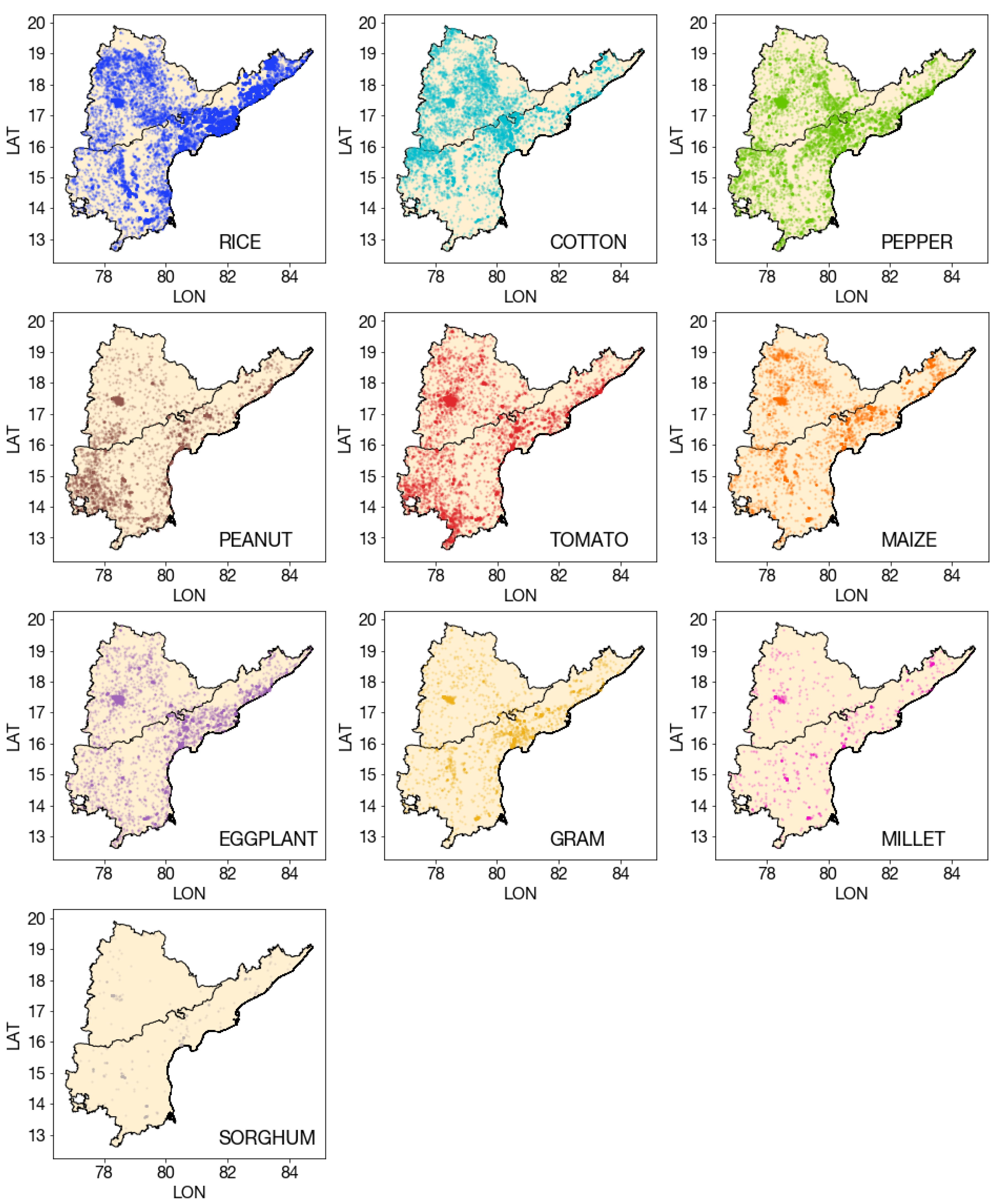
Figure A1.
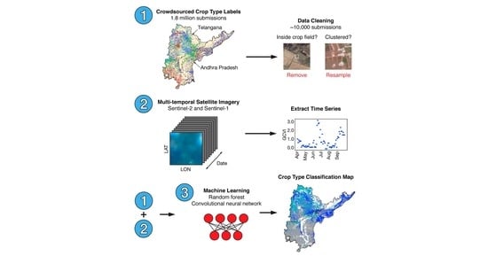
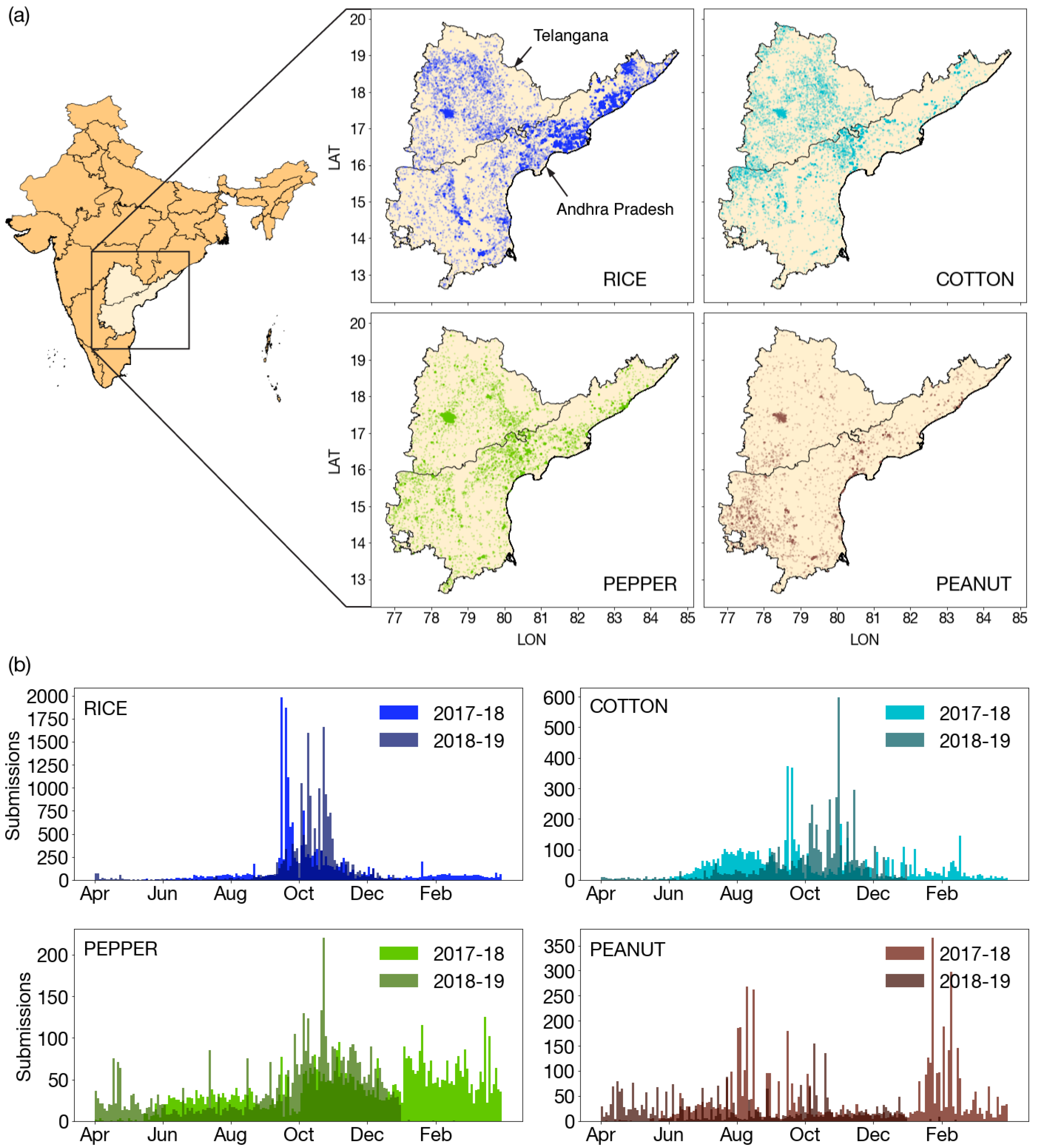
Geographic distribution of submissions for each crop type. Crops are ordered by number of submissions in the dataset, rice with the most and sorghum the least.
Figure A1.
Geographic distribution of submissions for each crop type. Crops are ordered by number of submissions in the dataset, rice with the most and sorghum the least.
Figure A2.
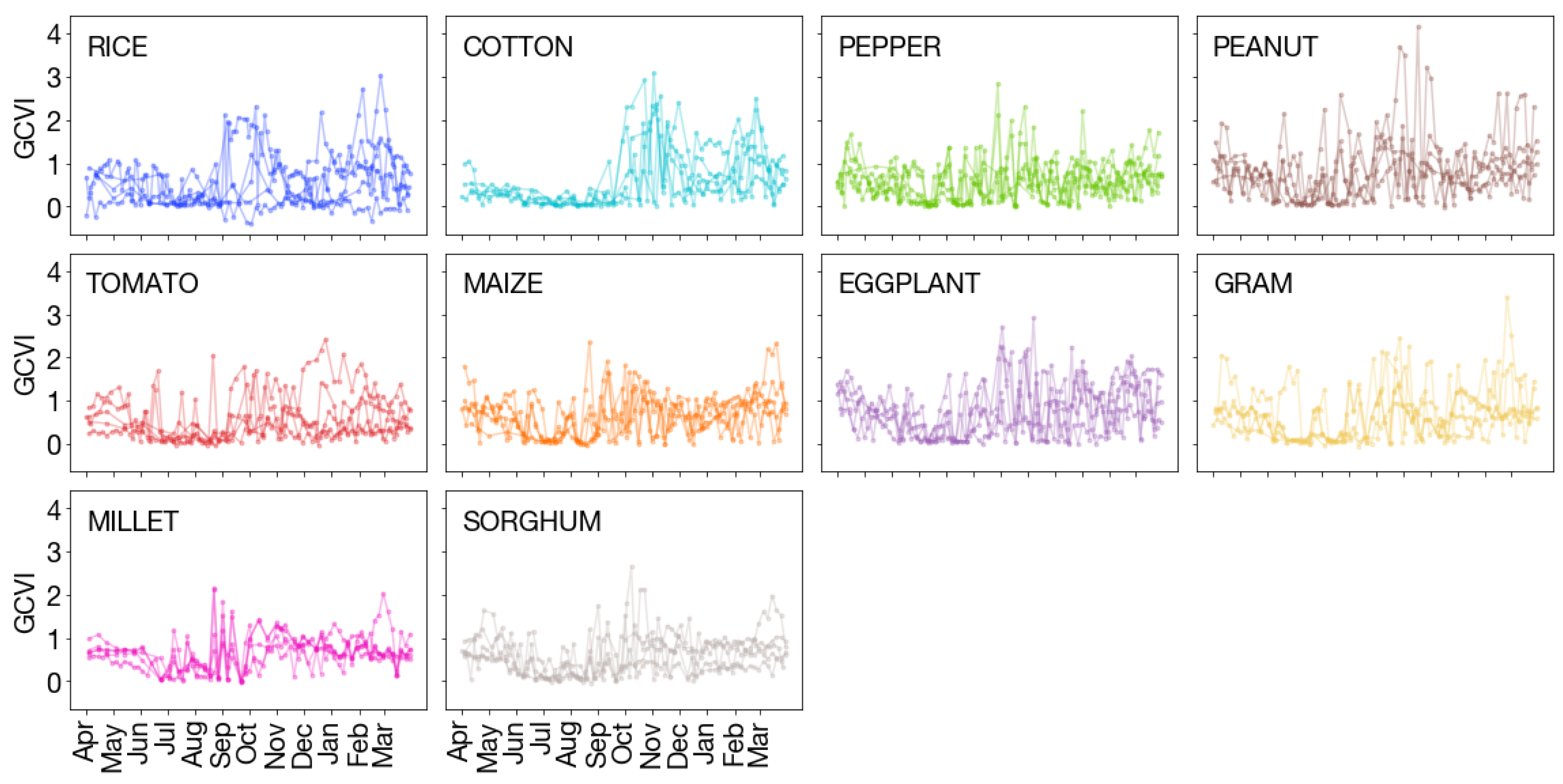
Sentinel-1 time series. For each crop type, VH/VV of Sentinel-1 time series at 5 randomly sampled submissions are shown from 1 April of the crop year to 31 March of the next year.
Figure A2.
Sentinel-1 time series. For each crop type, VH/VV of Sentinel-1 time series at 5 randomly sampled submissions are shown from 1 April of the crop year to 31 March of the next year.
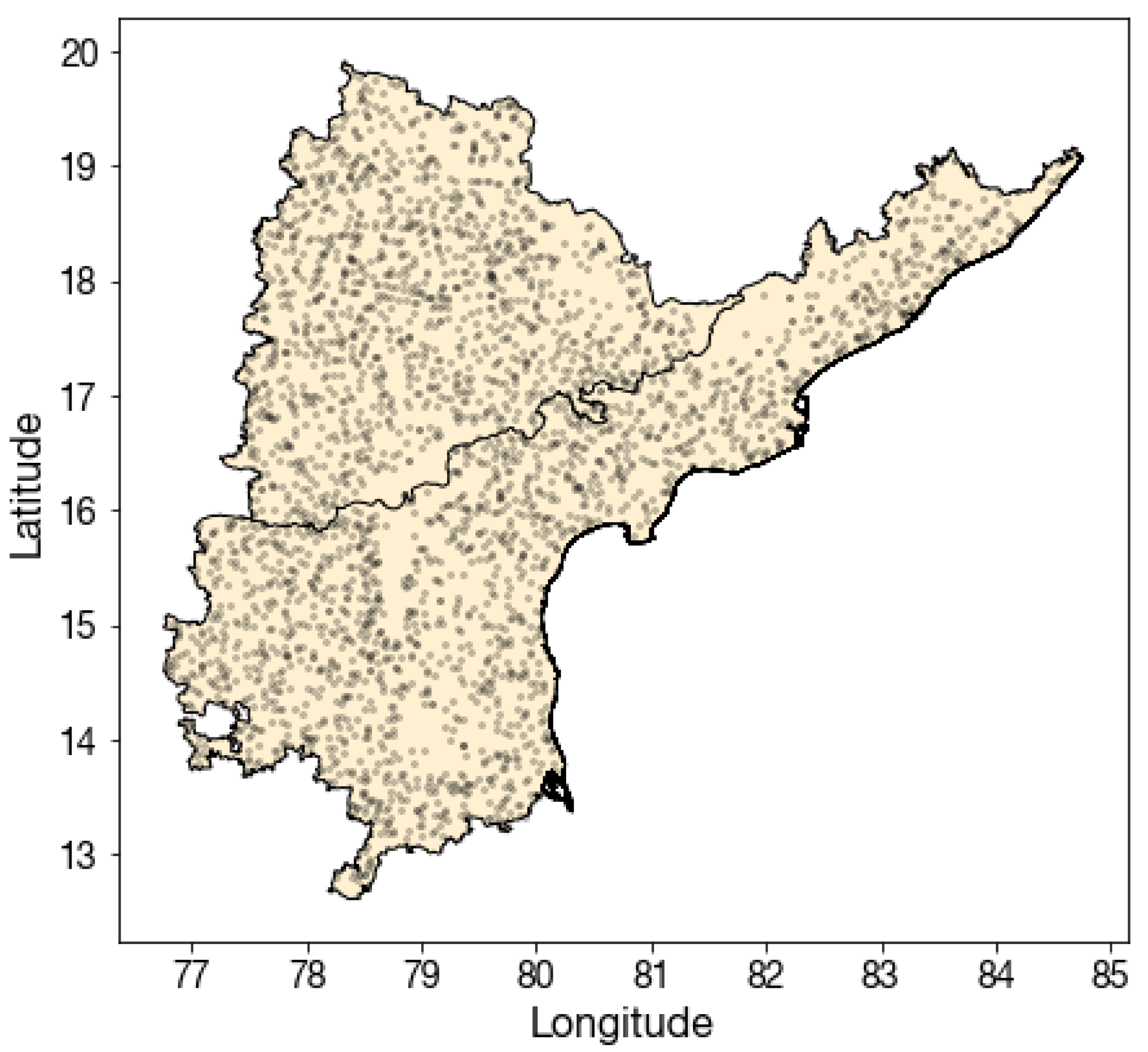
Figure A3.
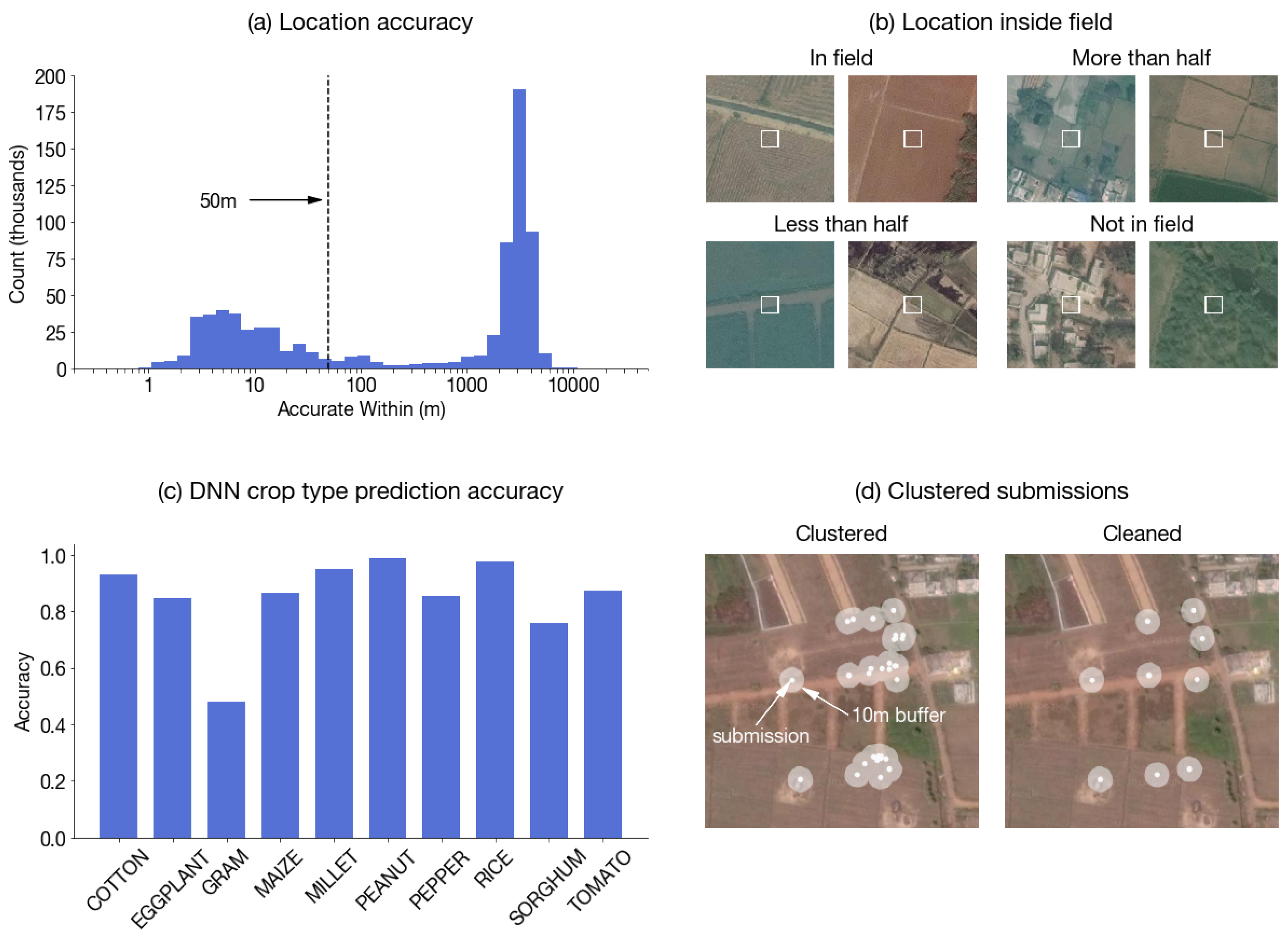
Map of 3000 submissions sampled for “in-field” labeling. The DigitalGlobe image ( pixels at 0.3 m resolution) centered at each location was downloaded and labeled for whether the center m box was inside a field.
Figure A3.
Map of 3000 submissions sampled for “in-field” labeling. The DigitalGlobe image ( pixels at 0.3 m resolution) centered at each location was downloaded and labeled for whether the center m box was inside a field.
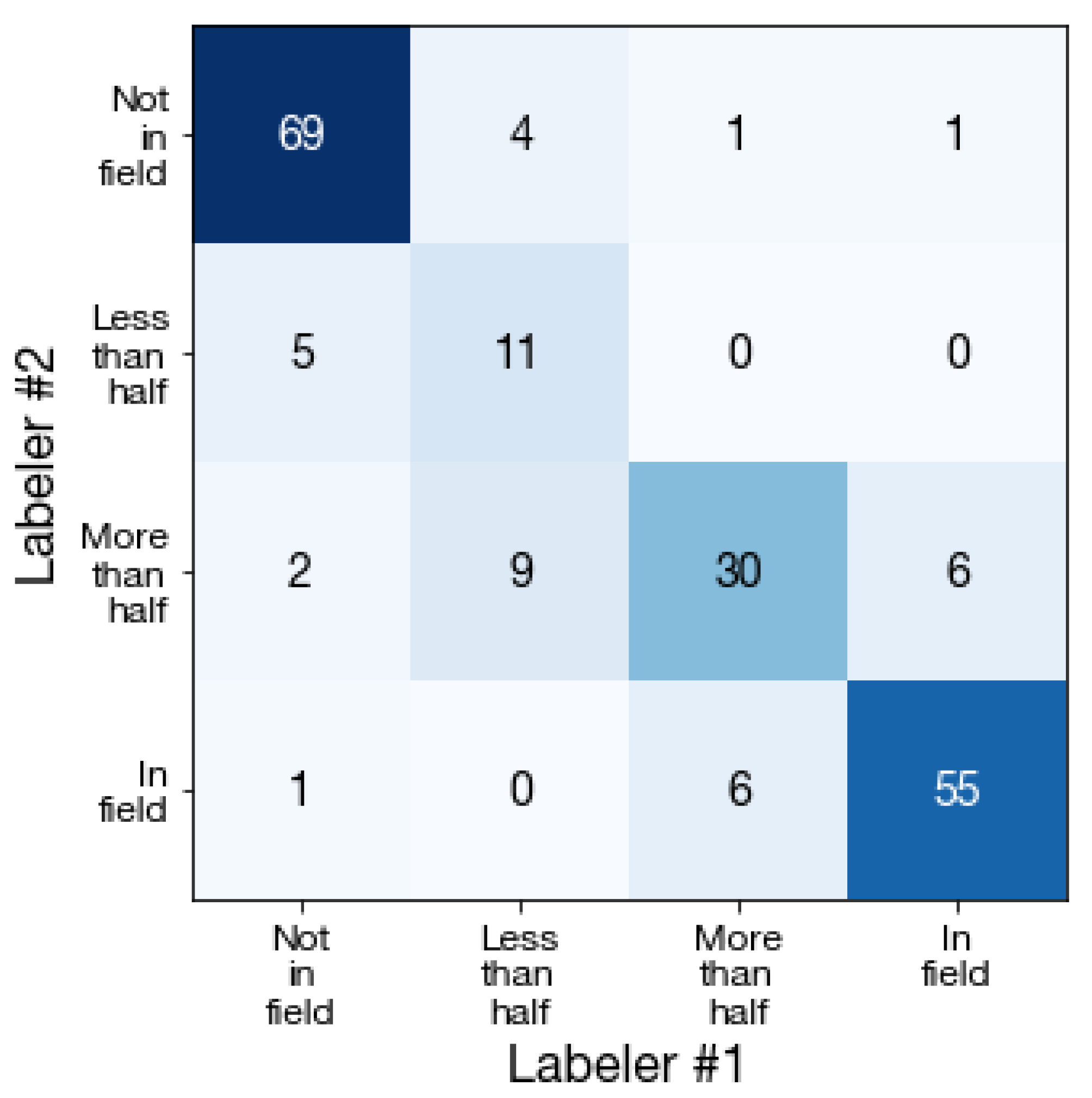
Figure A4.
Labeler agreement. Confusion matrix of in-field labels generated by two labelers on a subsample of 200 DigitalGlobe images. Percent agreement across 4 classes is 83%, and across 2 classes (more than half, less than half) is 93%.
Figure A4.
Labeler agreement. Confusion matrix of in-field labels generated by two labelers on a subsample of 200 DigitalGlobe images. Percent agreement across 4 classes is 83%, and across 2 classes (more than half, less than half) is 93%.
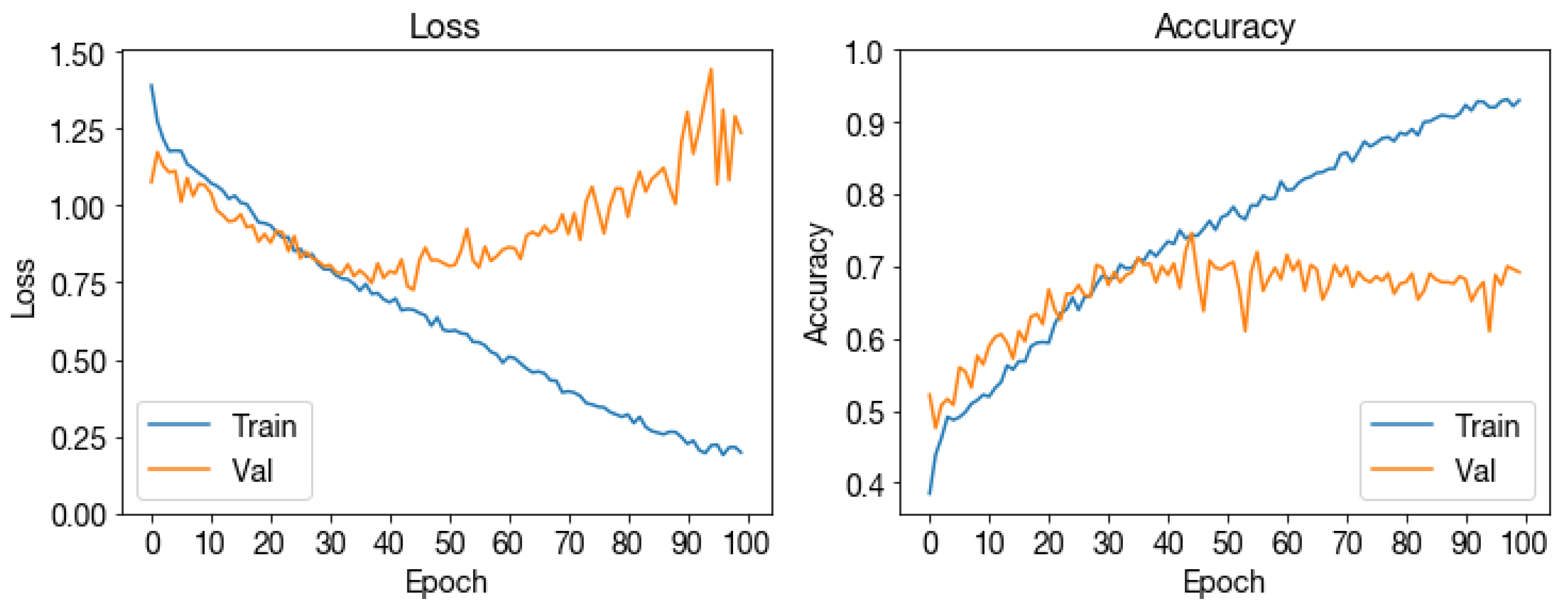
Figure A5.
Pretrained ResNet-18 loss and accuracy across training epochs.
Figure A5.
Pretrained ResNet-18 loss and accuracy across training epochs.
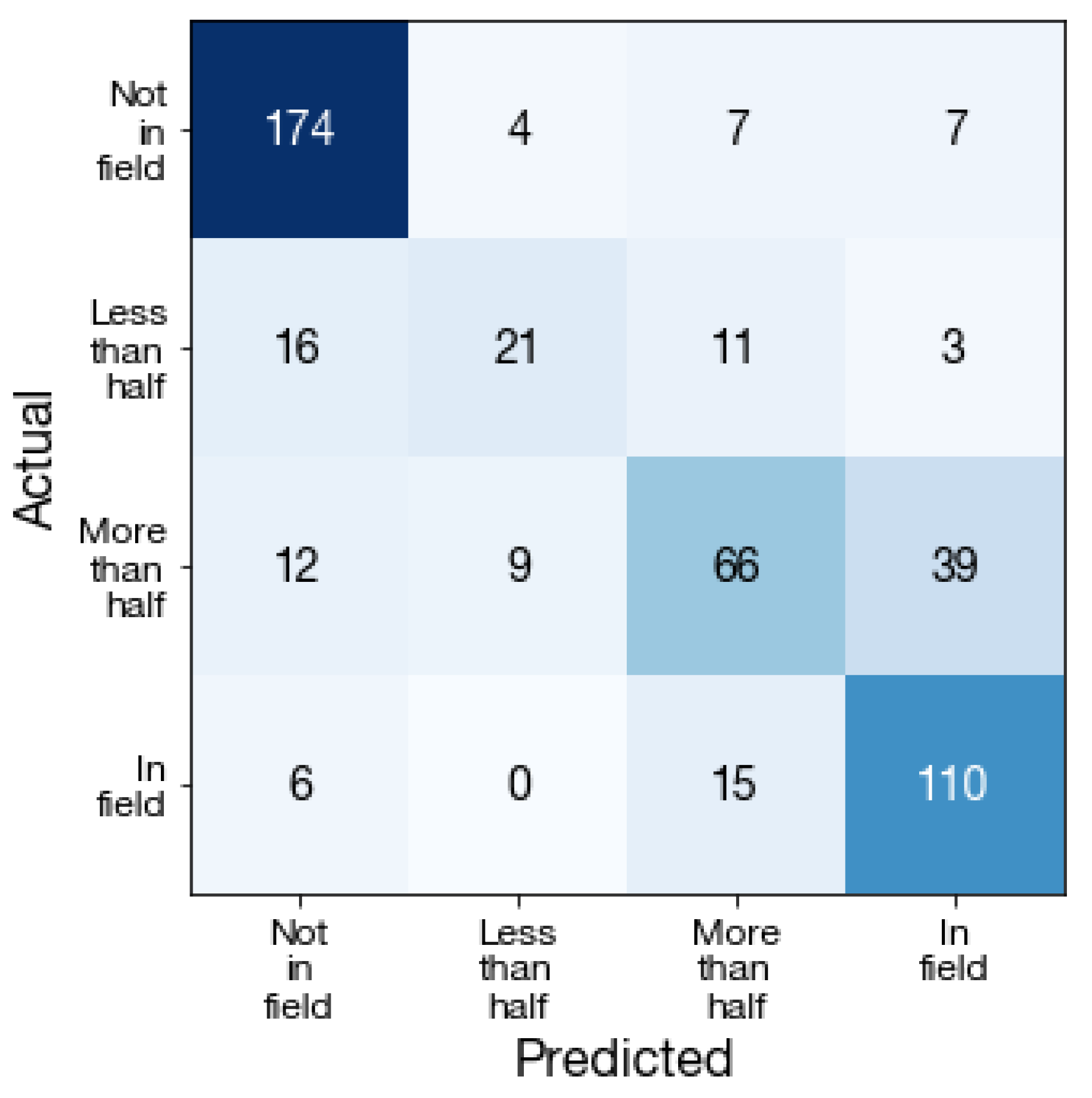
Figure A6.
In-field classification confusion matrix. Values are shown for test set.
Figure A6.
In-field classification confusion matrix. Values are shown for test set.
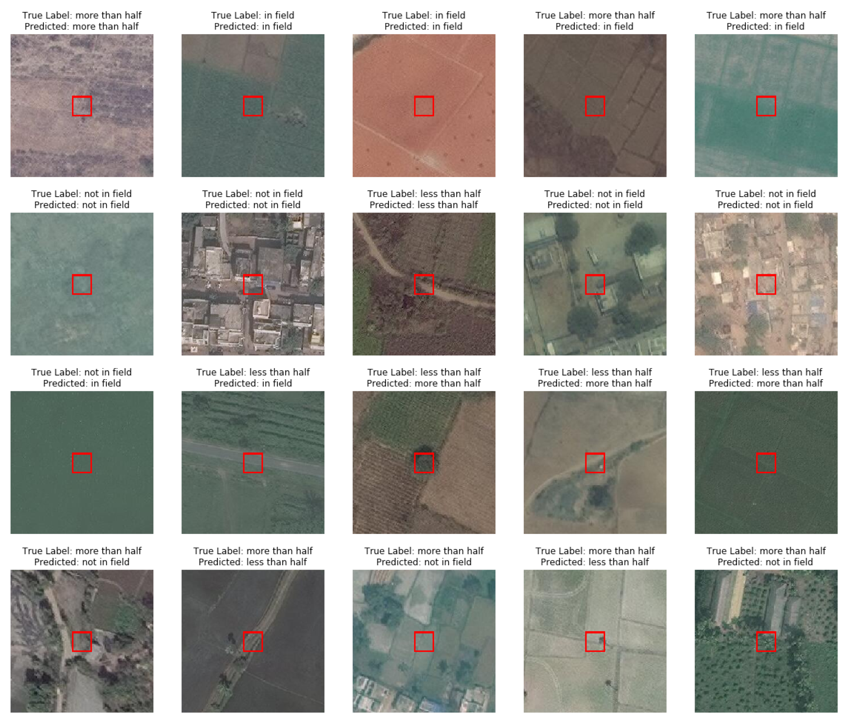
Figure A7.
From first row to last row: true positives, true negatives, false positives, and false negatives of the binary in-field classification problem. Five examples were sampled at random from each category. The box marks the size of a Sentinel-2 pixel.
Figure A7.
From first row to last row: true positives, true negatives, false positives, and false negatives of the binary in-field classification problem. Five examples were sampled at random from each category. The box marks the size of a Sentinel-2 pixel.
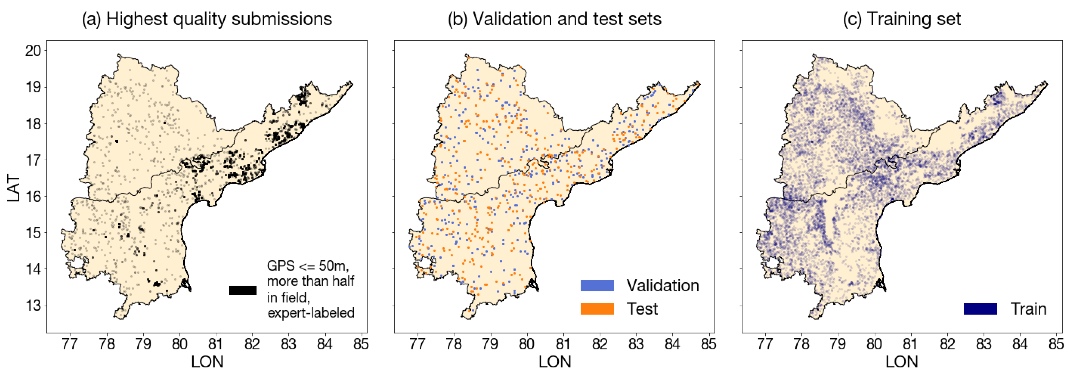
Figure A8.
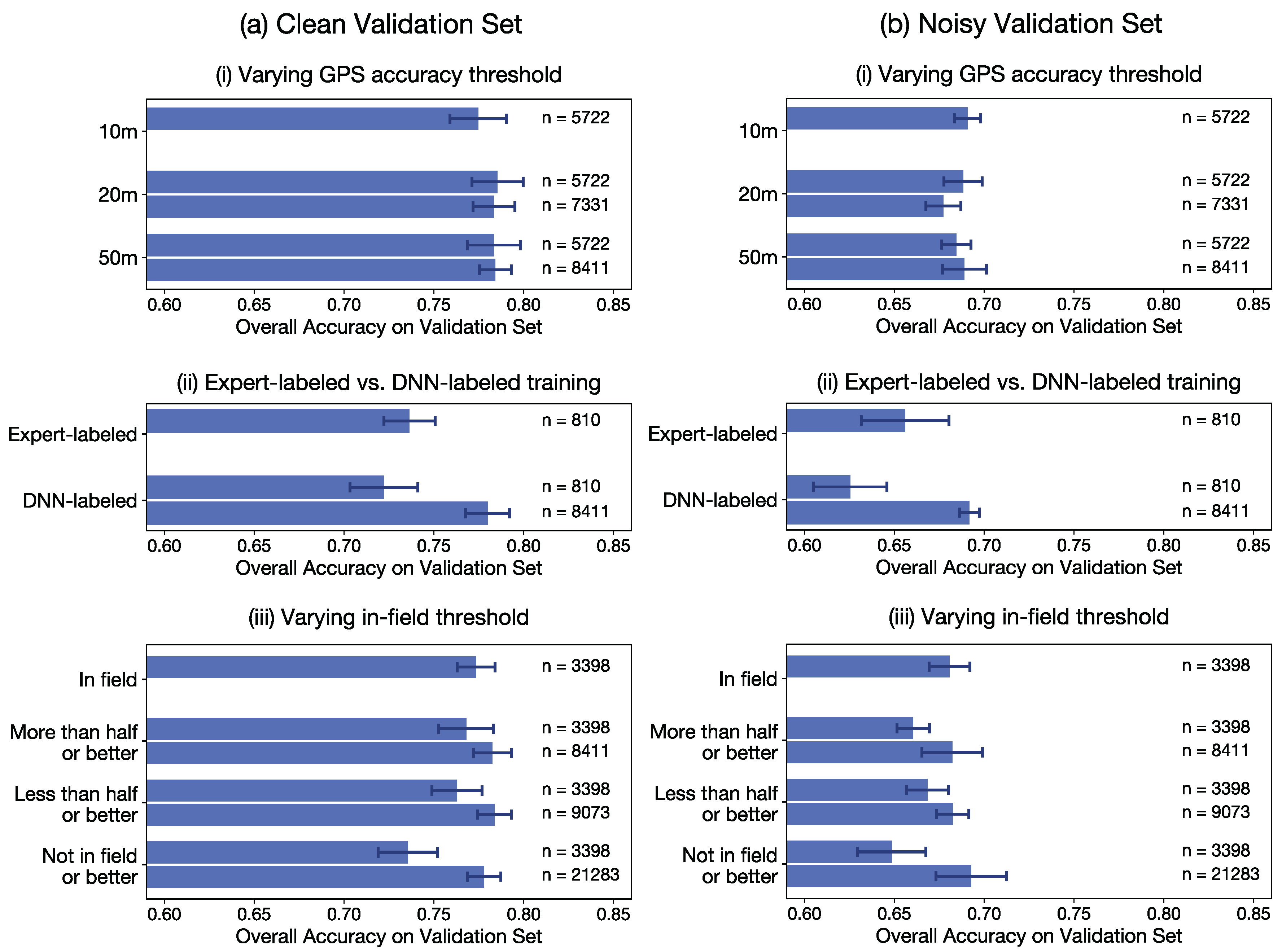
Maps of Plantix training, validation, and test sets for crop type classification. (a) To build the validation and test sets, we started with the highest quality submissions (GPS accuracy m, more than half of the Sentinel-2 pixel is in a field, crop type was assigned by a human expert). These submissions were highly concentrated in the eastern half of Andhra Pradesh. (b) High quality submissions were re-sampled in a spatially uniform way to form the validation and test sets ( for both). (c) The training set was filtered from the remaining dataset to be m away from any points in the validation and test sets, with GPS accuracy m and more than half of the Sentinel-2 pixel in a field.
Figure A8.
Maps of Plantix training, validation, and test sets for crop type classification. (a) To build the validation and test sets, we started with the highest quality submissions (GPS accuracy m, more than half of the Sentinel-2 pixel is in a field, crop type was assigned by a human expert). These submissions were highly concentrated in the eastern half of Andhra Pradesh. (b) High quality submissions were re-sampled in a spatially uniform way to form the validation and test sets ( for both). (c) The training set was filtered from the remaining dataset to be m away from any points in the validation and test sets, with GPS accuracy m and more than half of the Sentinel-2 pixel in a field.
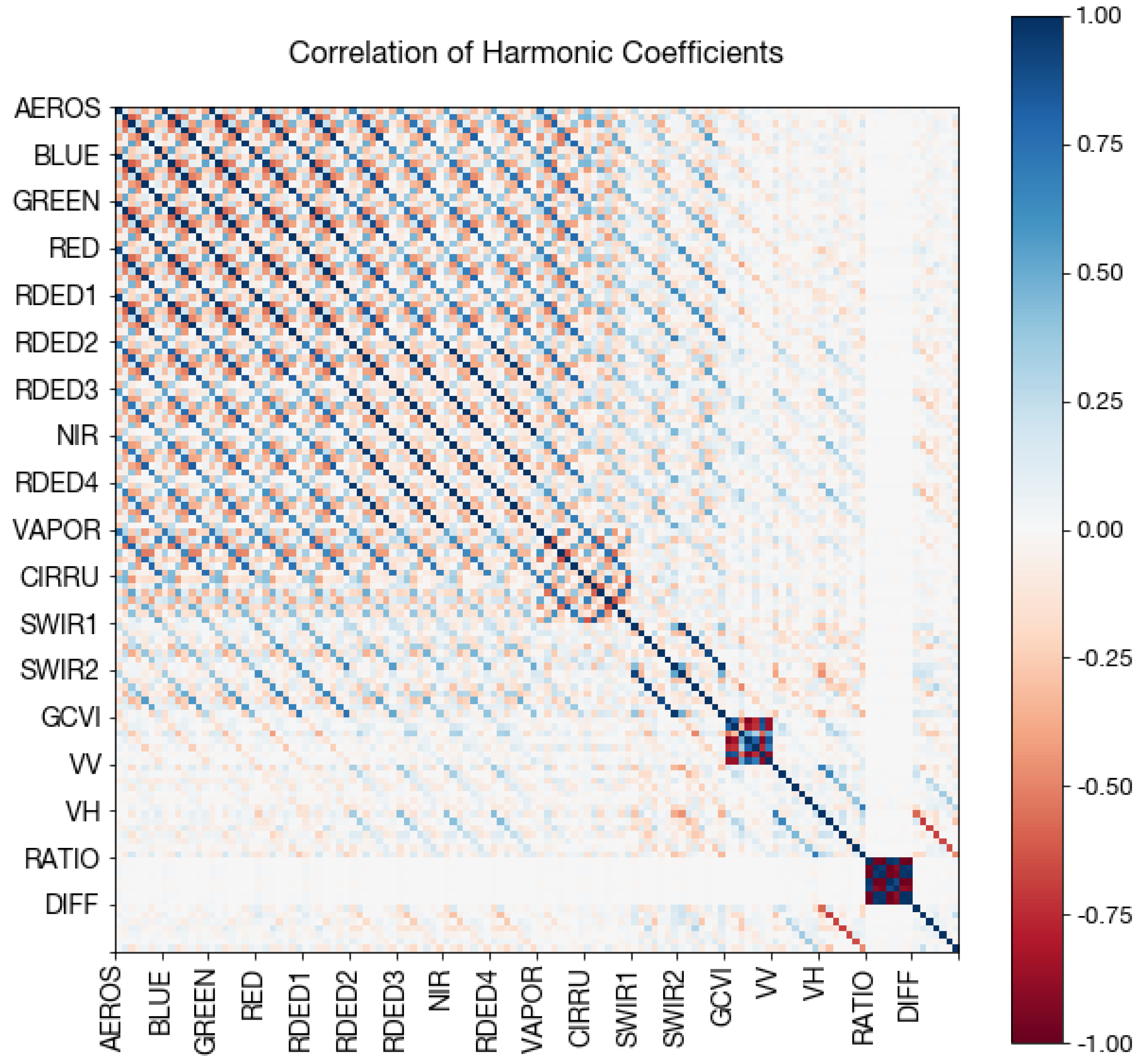
Figure A9.
Correlation matrix of harmonic coefficients. The 14 Sentinel-2 bands and 4 Sentinel-1 bands are shown. Within each band, coefficients are shown in order of ascending Fourier frequency, followed by the constant (
in Equation (
1)).
Figure A9.
Correlation matrix of harmonic coefficients. The 14 Sentinel-2 bands and 4 Sentinel-1 bands are shown. Within each band, coefficients are shown in order of ascending Fourier frequency, followed by the constant (
in Equation (
1)).
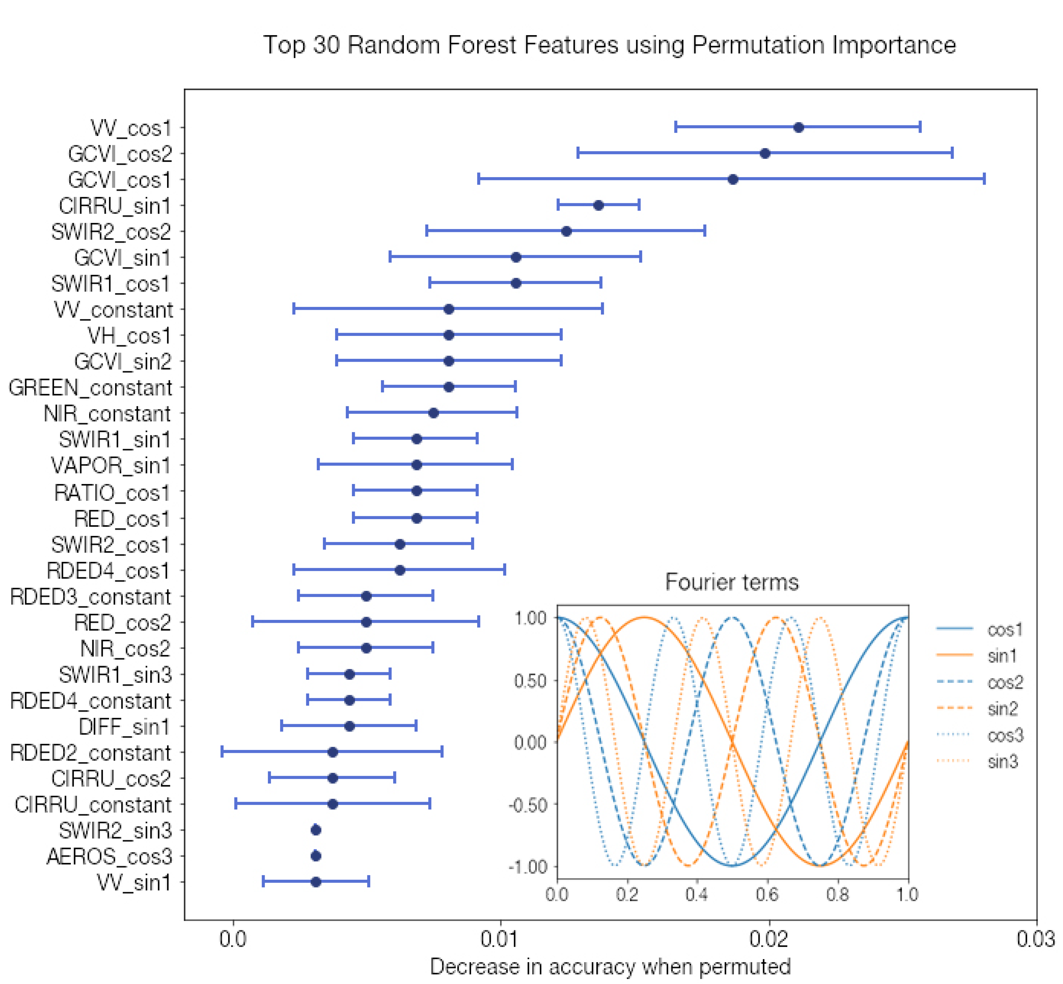
Figure A10.
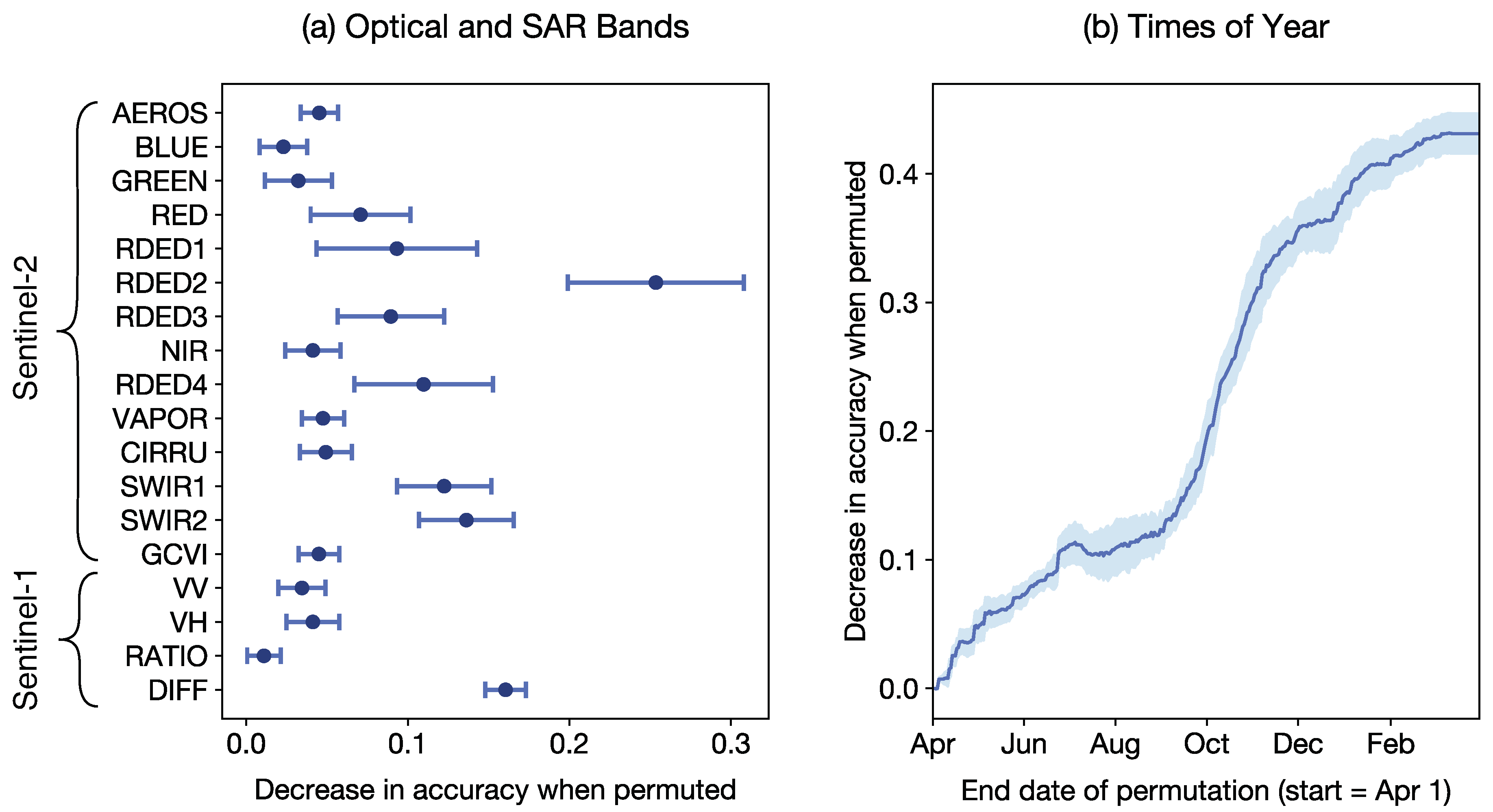
Harmonic coefficient feature importance via permutation. The permutation importance is shown for the 30 most important features. Error bars are 1 standard deviation. Fourier terms are shown in inset for reference.
Figure A10.
Harmonic coefficient feature importance via permutation. The permutation importance is shown for the 30 most important features. Error bars are 1 standard deviation. Fourier terms are shown in inset for reference.
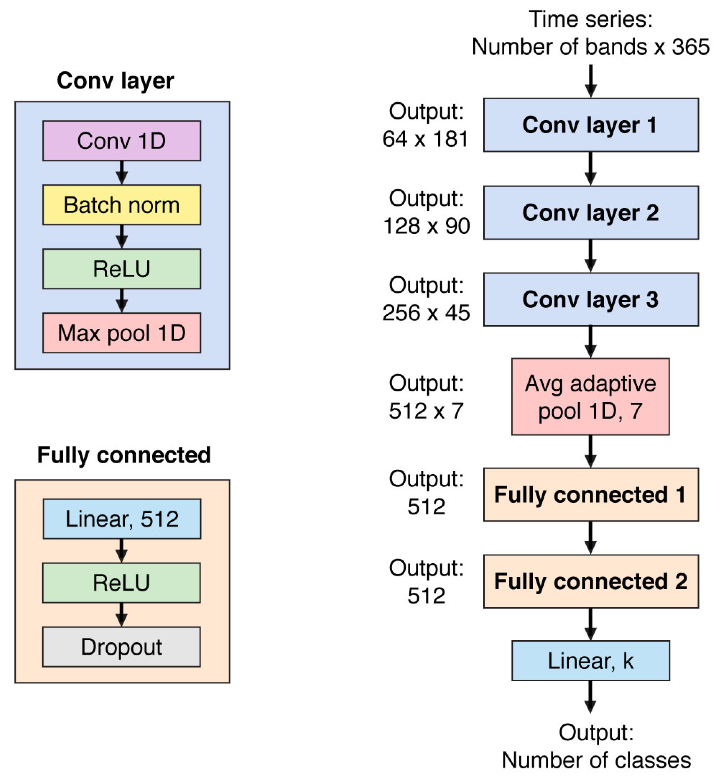
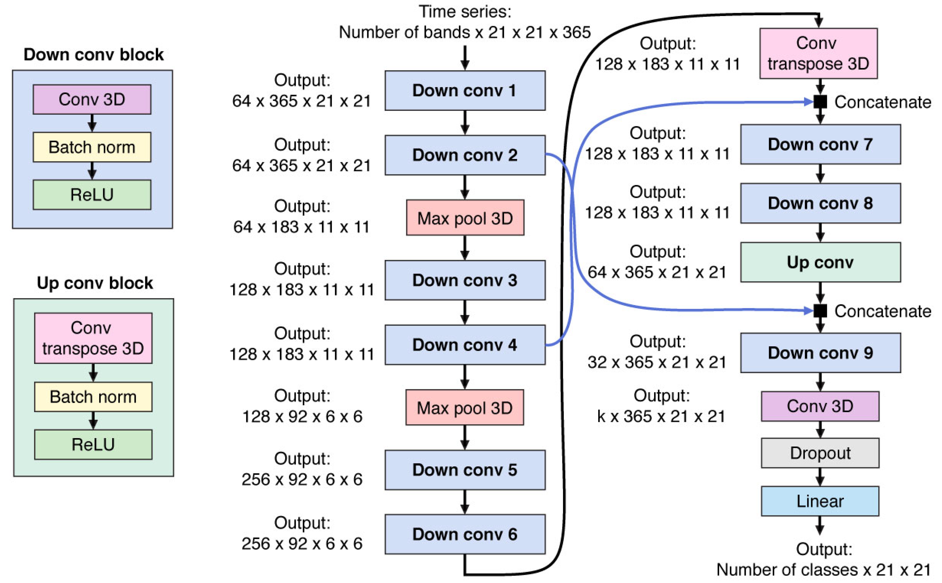
Figure A11.
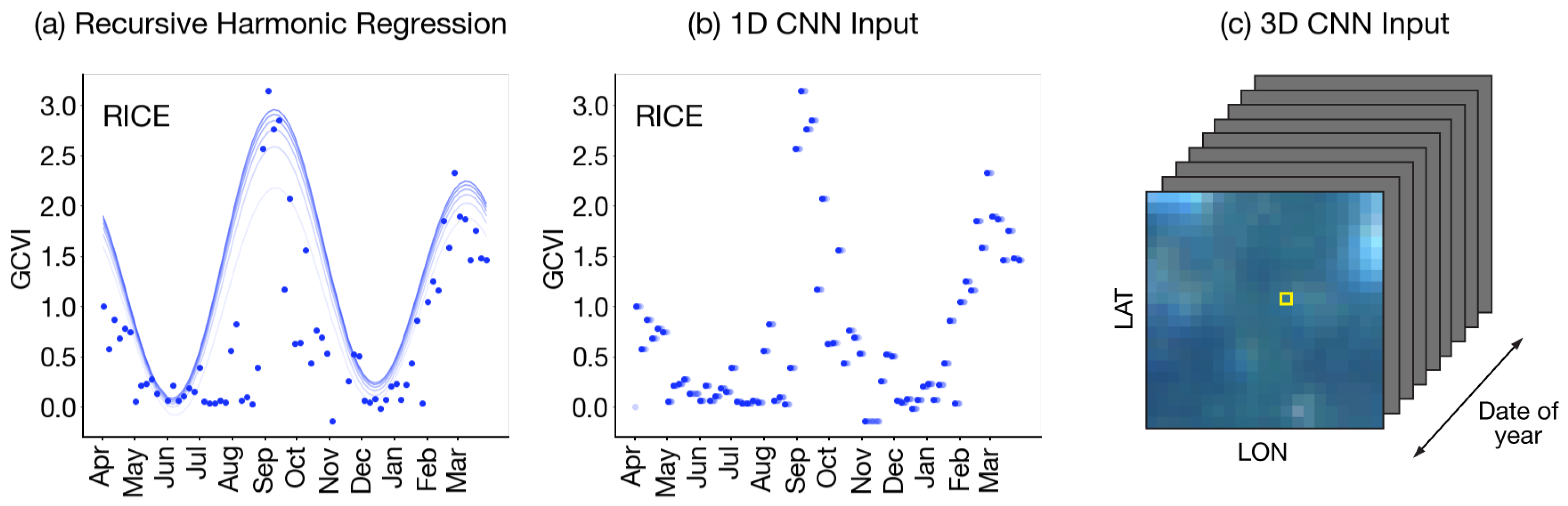
1D CNN architecture.
Figure A11.
1D CNN architecture.
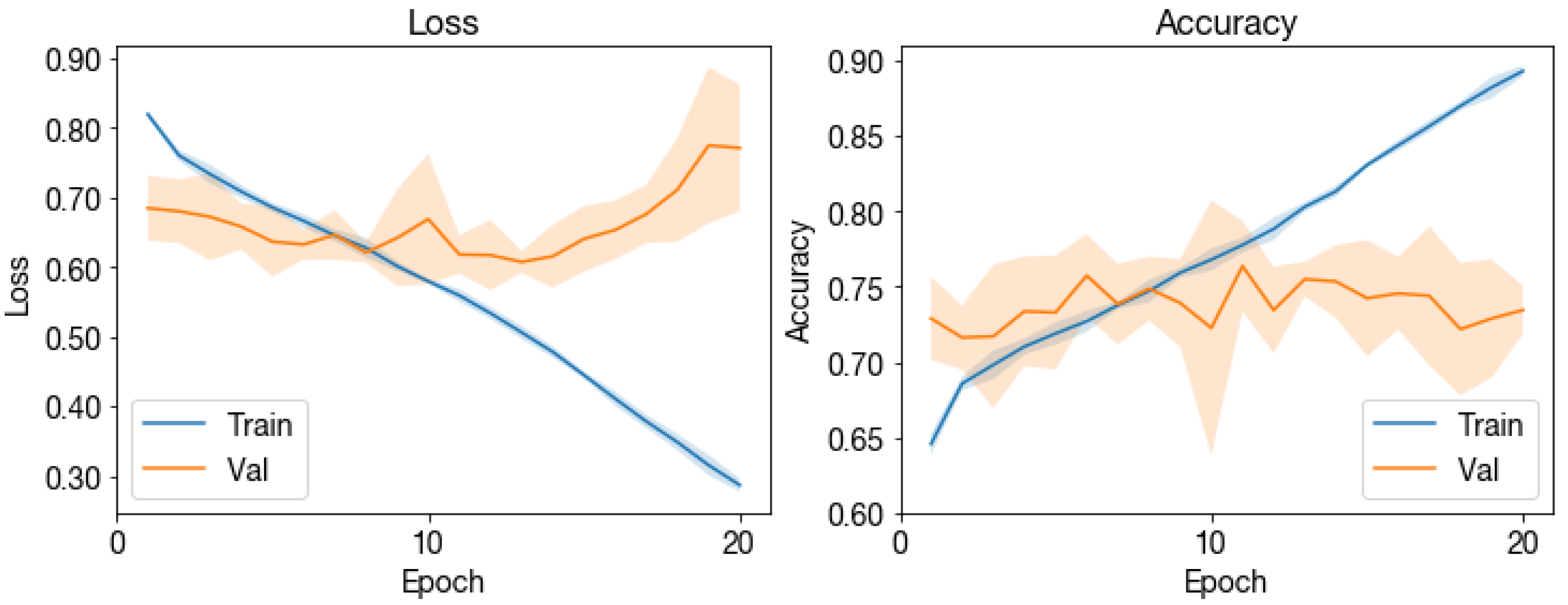
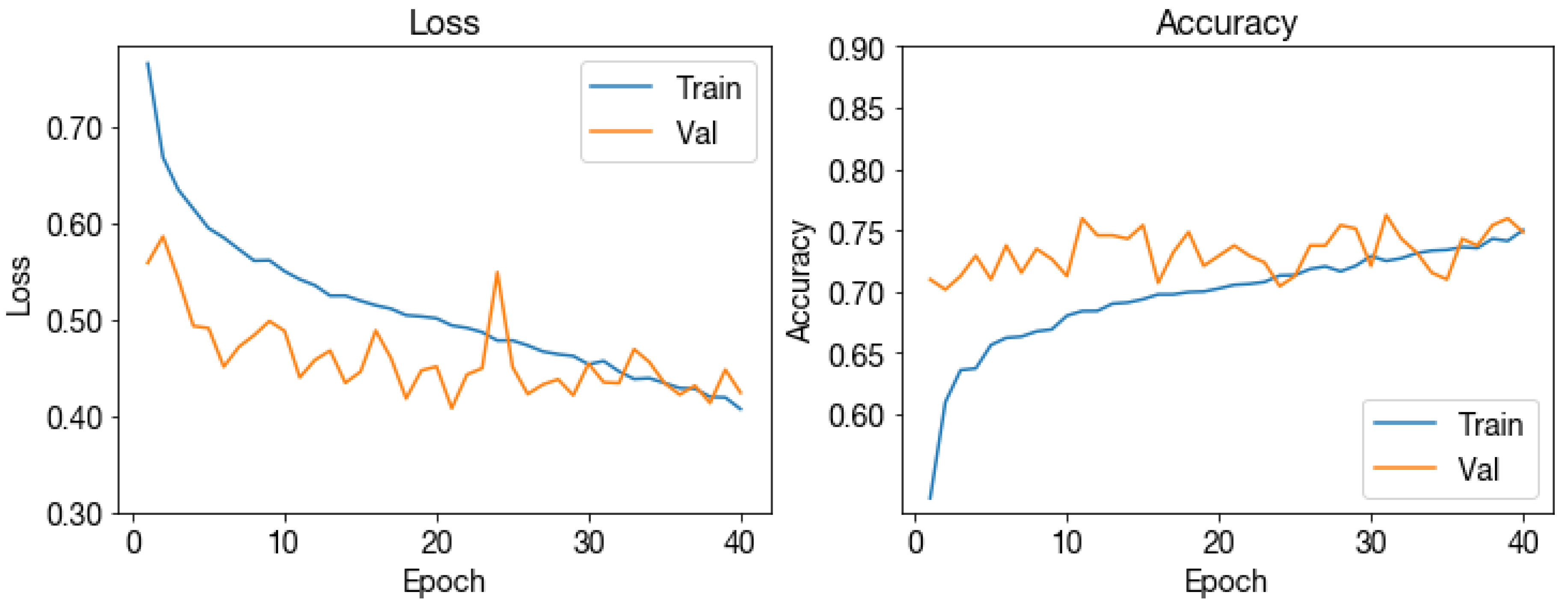
Figure A12.
1D CNN loss and accuracy across training epochs.
Figure A12.
1D CNN loss and accuracy across training epochs.
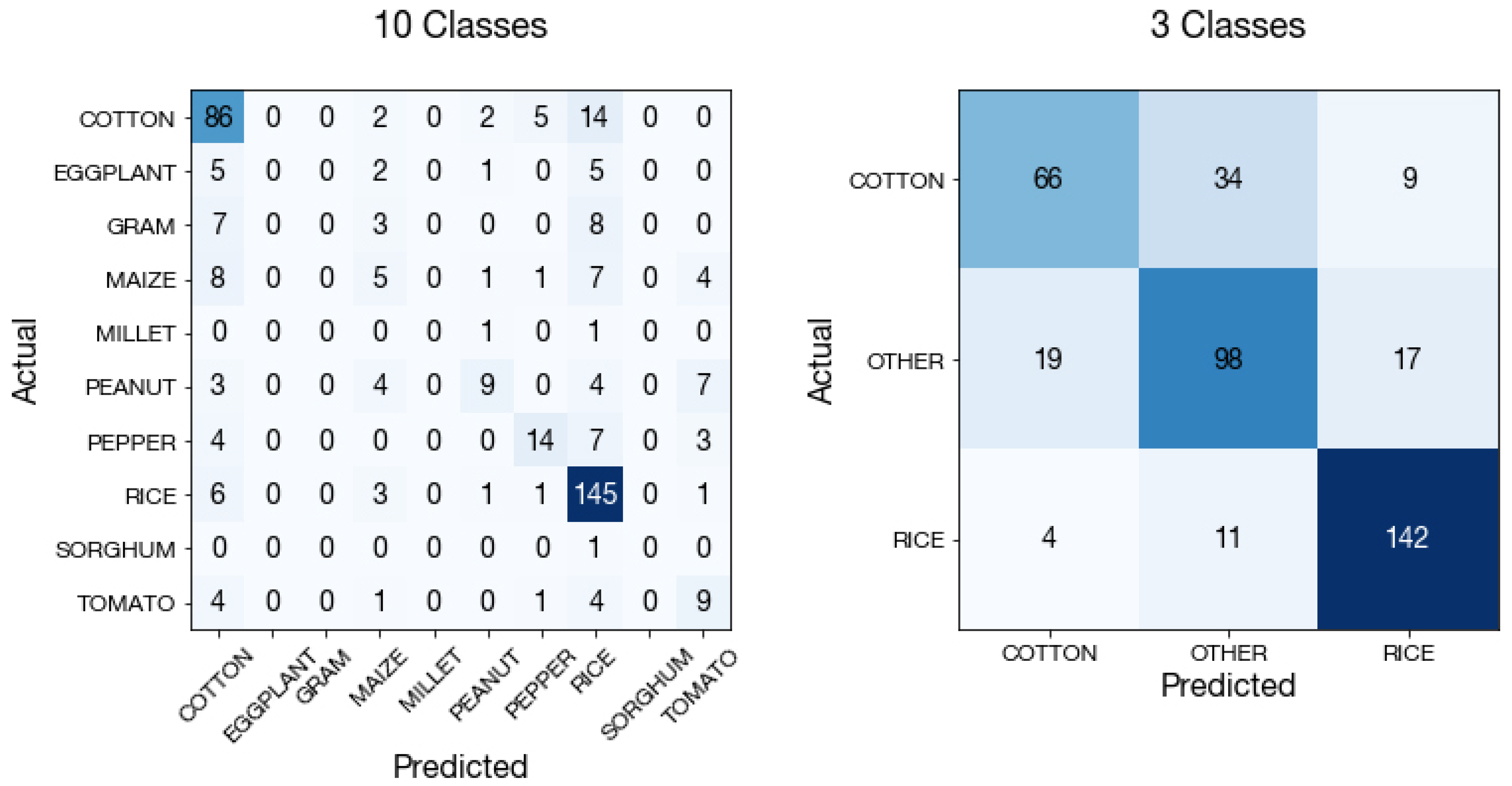
Figure A13.
Crop type classification confusion matrices on the 10-class task and the 3-class task. Values are shown for the test set ().
Figure A13.
Crop type classification confusion matrices on the 10-class task and the 3-class task. Values are shown for the test set ().
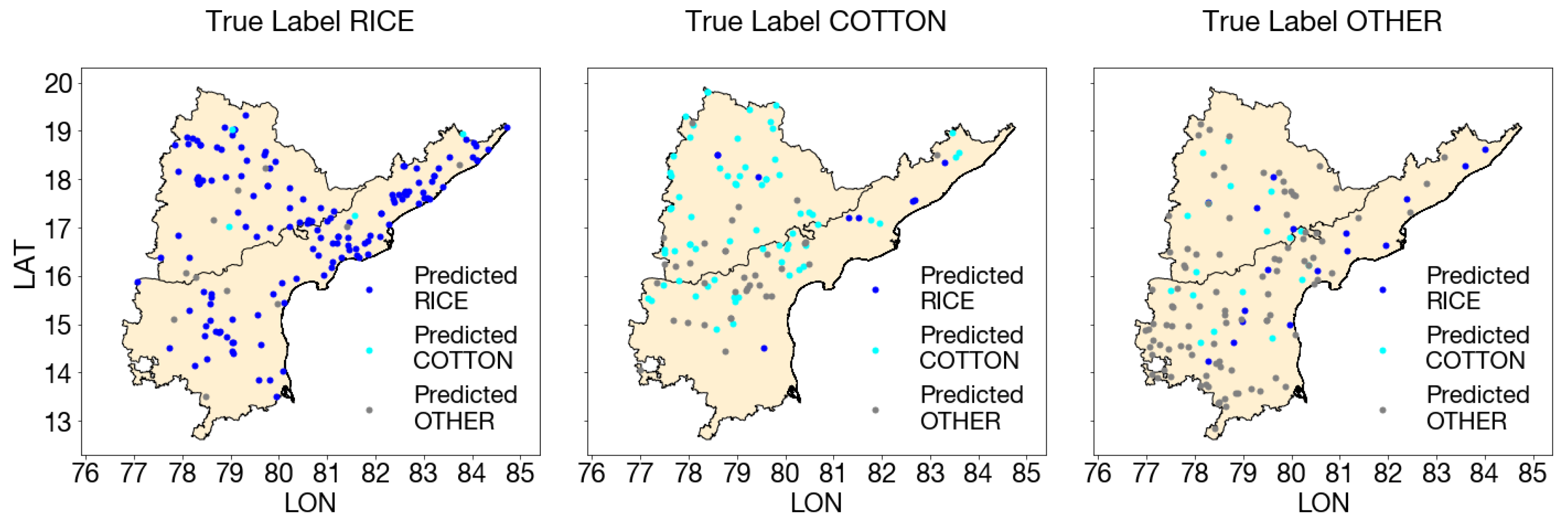
Figure A14.
Map of 1D CNN predictions for rice, cotton, and other kharif crops. From left to right: panels show our model’s predictions for test points whose true labels are rice, cotton, and other, respectively.
Figure A14.
Map of 1D CNN predictions for rice, cotton, and other kharif crops. From left to right: panels show our model’s predictions for test points whose true labels are rice, cotton, and other, respectively.
Figure A15.
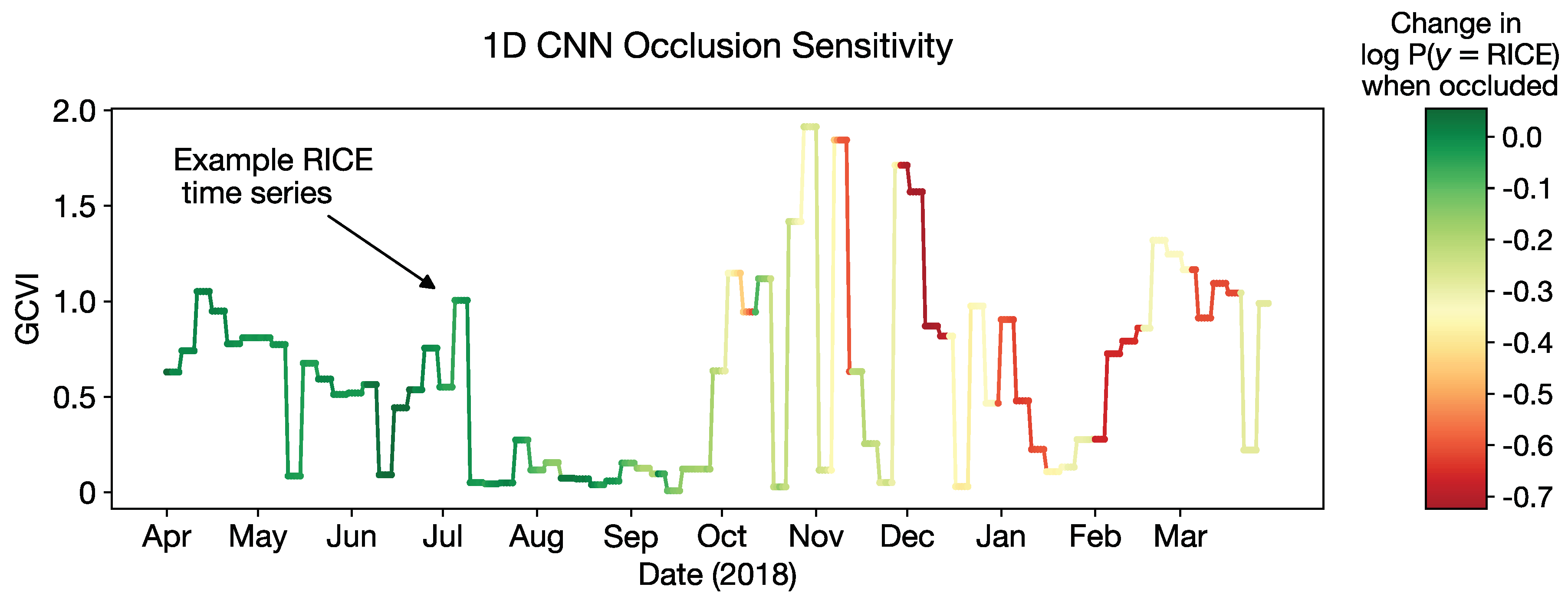
Occlusion sensitivity analysis. We blocked a 5-day sliding window of values in an example time series and analyzed its effect on the probability score output by the 1D CNN. The time series is originally correctly classified by the network as “rice”. The values substituted in the occlusion window are the mean of the time series. Only GCVI is visualized, but all Sentinel-2 and Sentinel-1 values in the window were occluded. Cloudy observations appear as low values in GCVI. The greater the decrease in (more red), the more the 1D CNN relies on that segment of the time series for classification. Conversely, greener segments are less important for classification.
Figure A15.
Occlusion sensitivity analysis. We blocked a 5-day sliding window of values in an example time series and analyzed its effect on the probability score output by the 1D CNN. The time series is originally correctly classified by the network as “rice”. The values substituted in the occlusion window are the mean of the time series. Only GCVI is visualized, but all Sentinel-2 and Sentinel-1 values in the window were occluded. Cloudy observations appear as low values in GCVI. The greater the decrease in (more red), the more the 1D CNN relies on that segment of the time series for classification. Conversely, greener segments are less important for classification.
Figure A16.
3D CNN architecture.
Figure A16.
3D CNN architecture.
Figure A17.
3D CNN loss and accuracy across training epochs.
Figure A17.
3D CNN loss and accuracy across training epochs.
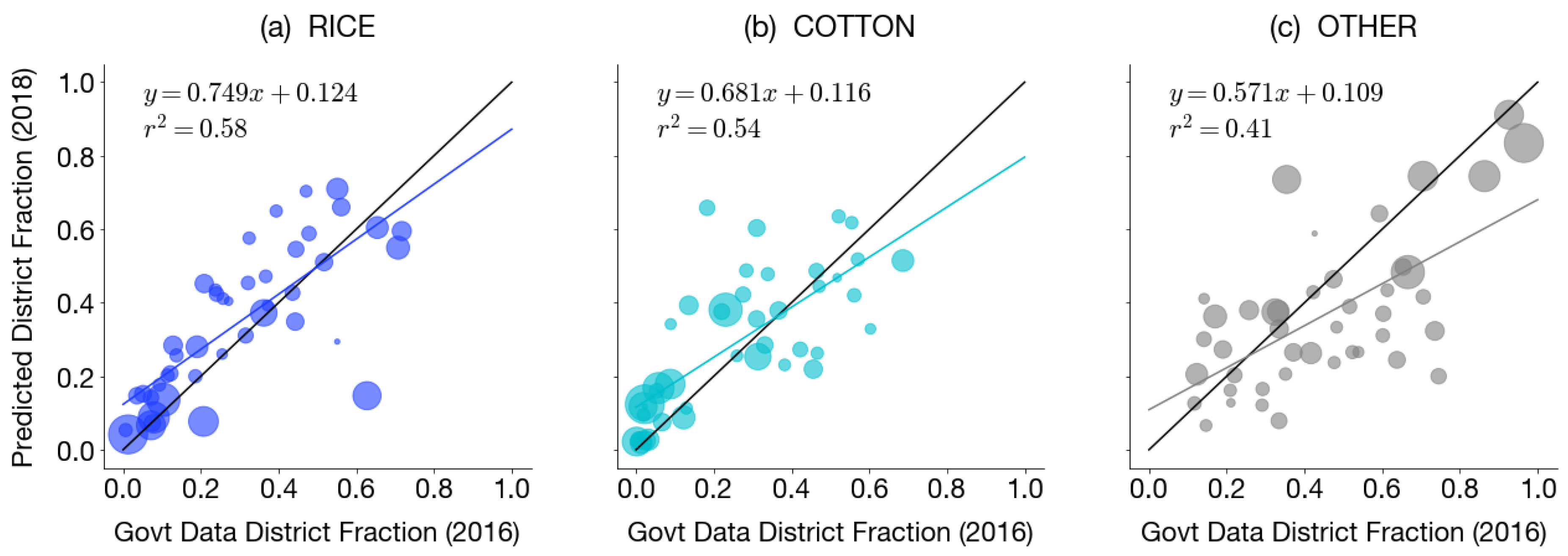
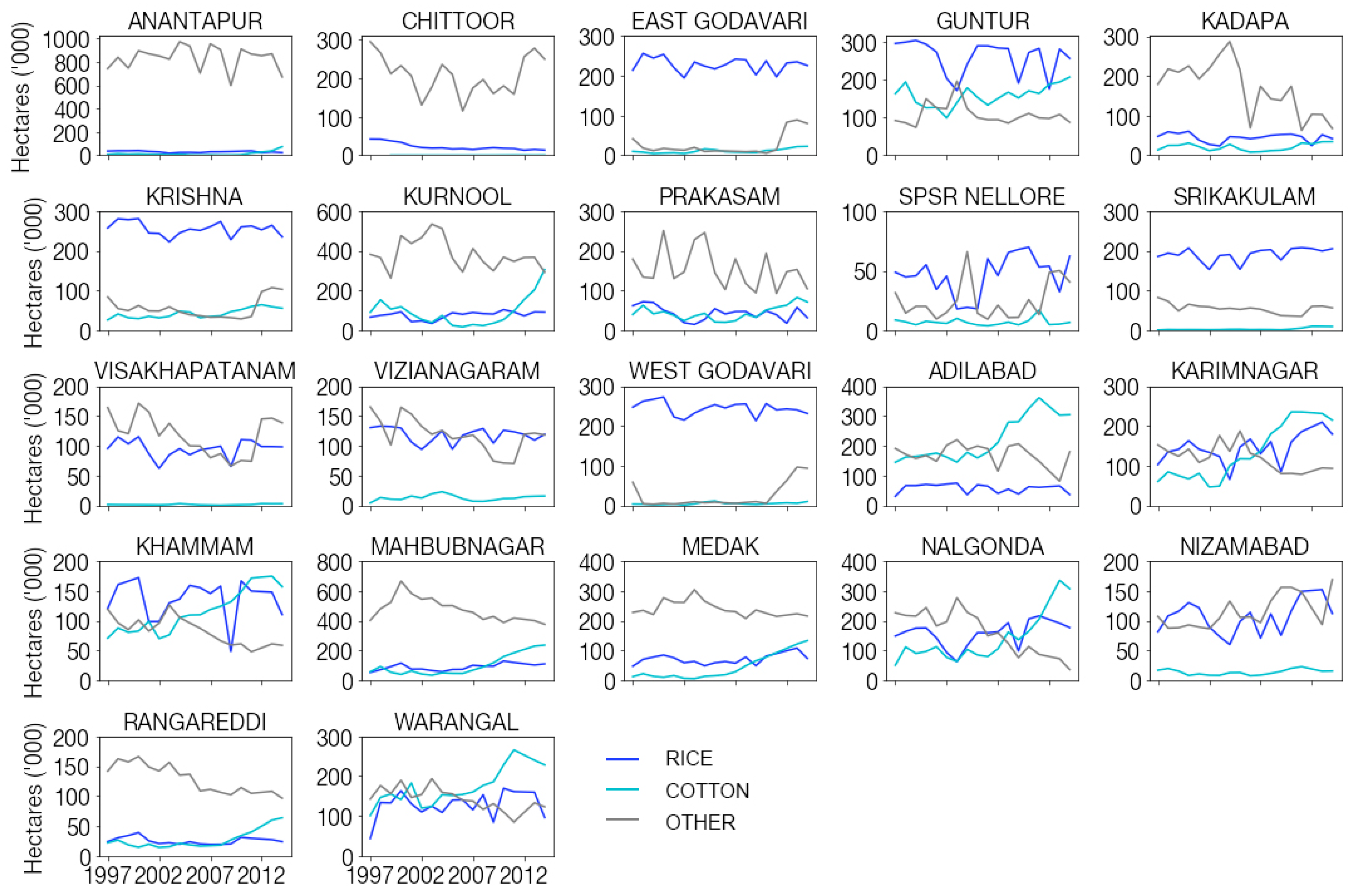
Figure A18.
District-level kharif crop area in Andhra Pradesh and Telangana from 1997–2014. Area data were downloaded from
data.gov.in and are shown for rice, cotton, and other, where other shows the sum of non-rice and non-cotton crops.
Figure A18.
District-level kharif crop area in Andhra Pradesh and Telangana from 1997–2014. Area data were downloaded from
data.gov.in and are shown for rice, cotton, and other, where other shows the sum of non-rice and non-cotton crops.
Table A1.
Pretrained CNN implementation details. Hyperparameters for the pretrained 2D CNNs used for in-field classification. We refer the reader to references [
54,
55] for descriptions of the architectures of VGG and ResNet CNNs.
Table A1.
Pretrained CNN implementation details. Hyperparameters for the pretrained 2D CNNs used for in-field classification. We refer the reader to references [
54,
55] for descriptions of the architectures of VGG and ResNet CNNs.
| Model | Hyperparameter | Value |
|---|
| VGG [54] | Input size | |
| Kernel size | |
| Initial filters | 16 |
| Batch size | 4 |
| Epochs | 200 |
| Optimizer | SGD |
| Learning rate | 0.0001 |
| Momentum | 0.9 |
| ResNet [55] | Input size | |
| Kernel size | , |
| Initial filters | 64 |
| Batch size | 4 |
| Epochs | 100 |
| Optimizer | Adam |
| Learning rate | 0.001 |
| Betas | (0.9, 0.999) |
| All | Brightness jitter | 0.5 |
| Contrast jitter | 0.5 |
| Saturation jitter | 0.5 |
| Hue jitter | 0 |
Table A2.
In-field model selection. VGG and ResNet training and validation accuracies are shown for 12 architecture and hyperparameter settings. Comparisons to guessing everything is in the majority class (not in field) and human labeler accuracy are provided to gauge task difficulty and lower/upper bounds for metrics. Test accuracy was computed for the model with highest validation accuracy.
| Model | Layers | GSD | Best | Training | Validation | Test |
|---|
| -Reg | Accuracy | Accuracy | Accuracy |
|---|
| Majority class | – | – | – | 0.388 | 0.368 | 0.384 |
| VGG (pretrained) | 11 | 0.3 m | 0.0 | 0.704 | 0.708 | |
| | 0.6 m | 0.0 | 0.794 | 0.730 | |
| 19 | 0.3 m | 0.0 | 0.727 | 0.722 | |
| | 0.6 m | 0.0 | 0.837 | 0.736 | |
| ResNet (pretrained) | 18 | 0.3 m | 0.0 | 0.743 | 0.746 | 0.742 |
| | 0.6 m | 0.0 | 0.744 | 0.716 | |
| 50 | 0.3 m | 0.0 | 0.722 | 0.694 | |
| | 0.6 m | 0.0 | 0.718 | 0.710 | |
VGG
(not pretrained) | 11 | 0.3 m | 0.0 | 0.761 | 0.722 | |
| | 0.6 m | 0.0 | 0.720 | 0.712 | |
ResNet
(not pretrained) | 18 | 0.3 m | 0.0 | 0.770 | 0.680 |
| | 0.6 m | 0.0 | 0.771 | 0.686 | |
| Human labeler | – | 0.3 m | – | 0.825 | 0.825 | 0.825 |
Table A3.
Data storage and computational runtime required of the 3 machine learning algorithms. Data storage is shown for 10,000 samples. Experiment runtimes are shown for the 3-class task for training and validating on a single model. Random forest experiments were performed using sklearn’s RandomForestClassifier with 500 trees on 8 CPUs with 52 GB RAM running Ubuntu 16.04. The CNNs were run on the same machine on one NVIDIA Tesla K80 GPU, and runtimes are shown for 20 epochs.
| | Harmonics and | 1D CNN | 3D CNN |
|---|
| | Random Forest |
|---|
| Sentinel-2 data storage | 27 MB | 406 MB | 166 GB |
| Sentinel-1 data storage | 8 MB | 116 MB | – |
| Number of parameters | – | | |
| Runtime (HH:mm:ss) | 00:00:40 | 00:02:22 | 44:00:00 |
Table A4.
Harmonics hyperparameter tuning. Grid search was performed to find the best pair of hyperparameters: the number of cosine and sine terms (order) and number of recursive fits. Each combination of hyperparameters was trained with 10 random bootstrapped training sets to obtain error bars (shown for 1 standard deviation). Random forest hyperparameters were kept at default based on previous work [
36], except number of trees was increased to 500.
| Model | Order | Number | Training | Validation |
|---|
| of Fits | Accuracy | Accuracy |
|---|
| Majority class | – | – | 0.322 | 0.399 |
| Harmonic features and random forest | 2 | 1 | | |
| | 2 | | |
| | 4 | | |
| | 8 | | |
| | 16 | | |
| 3 | 1 | | |
| | 2 | | 0.750 ± 0.008 |
| | 4 | | |
| | 8 | | |
| | 16 | | |
| 4 | 1 | | |
| | 2 | | |
| | 4 | | |
| | 8 | | |
| | 16 | | |
Table A5.
1D CNN implementation details. Hyperparameters for the 1D CNN yielding the highest validation set accuracy.
Table A5.
1D CNN implementation details. Hyperparameters for the 1D CNN yielding the highest validation set accuracy.
| Hyperparameter | Value |
|---|
| Kernel size | 3 |
| Conv layers | 4 |
| Initial filters | 64 |
| regularization | 0.0 |
| Batch size | 4 |
| Optimizer | Adam |
| Learning rate | 0.001 |
| Betas | (0.9, 0.999) |
Table A6.
1D CNN hyperparameter tuning. Due to the large search space, 24 sets of hyperparameters were randomly sampled from the grid of options, and each set was trained with 5 random CNN weight initializations and bootstrapped training sets to obtain error bars (shown for 1 standard deviation).
Table A6.
1D CNN hyperparameter tuning. Due to the large search space, 24 sets of hyperparameters were randomly sampled from the grid of options, and each set was trained with 5 random CNN weight initializations and bootstrapped training sets to obtain error bars (shown for 1 standard deviation).
| Model | Encoding | Layers | Initial | Learning | Batch | Training | Validation |
|---|
| Filters | Rate | Size | Accuracy | Accuracy |
|---|
| Majority class | – | – | – | – | – | 0.322 | 0.399 |
| 1D CNN | Constant until updated | 3 | 16 | 0.001 | 4 | | |
| | 64 | 0.0001 | 4 | | |
| 4 | 8 | 0.0001 | 16 | | |
| | | 0.001 | 16 | | |
| | 32 | 0.01 | 4 | | |
| | 64 | 0.001 | 16 | | 0.787 ± 0.010 |
| 5 | 8 | 0.001 | 16 | | |
| | 16 | 0.0001 | 4 | | |
| | 32 | 0.0001 | 16 | | |
| 6 | 8 | 0.001 | 4 | | |
| | | | 16 | | |
| | 32 | 0.001 | 4 | | |
| Zero for missing | 3 | 16 | 0.0001 | 4 | | |
| | 64 | 0.0001 | 4 | | |
| 4 | 8 | 0.001 | 4 | | |
| 5 | 8 | 0.0001 | 4 | | |
| | 32 | 0.0001 | 16 | | |
| | | 0.001 | 16 | | |
| | | 0.01 | 16 | | |
| | 64 | 0.001 | 16 | | |
| 6 | 8 | 0.001 | 16 | | |
| | 32 | 0.0001 | 16 | | |
| | 64 | 0.001 | 4 | | |
| | | 0.01 | 4 | | |
Table A7.
The additional value of Sentinel-1. Training and validation accuracies for the 10-crop classification problem and 3-class problem are compared between models using both SAR and optical (Sentinel-1 and -2) satellite imagery and only optical satellite imagery (Sentinel-2).
Table A7.
The additional value of Sentinel-1. Training and validation accuracies for the 10-crop classification problem and 3-class problem are compared between models using both SAR and optical (Sentinel-1 and -2) satellite imagery and only optical satellite imagery (Sentinel-2).
| Model | Number | Satellite(s) | Training | Validation |
|---|
| of Classes | Accuracy | Accuracy |
|---|
| Majority | 10 | – | 0.322 | 0.399 |
| class | 3 | – | 0.450 | 0.388 |
| Harmonics + random forest | 10 | Sentinel-1 and -2 | | |
| | Sentinel-2 | | |
| 3 | Sentinel-1 and -2 | | |
| | Sentinel-2 | | |
| 1D CNN | 10 | Sentinel-1 and -2 | | |
| | Sentinel-2 | | |
| 3 | Sentinel-1 and -2 | | |
| | Sentinel-2 | | |

 ,
, 


