A Hybrid Data Balancing Method for Classification of Imbalanced Training Data within Google Earth Engine: Case Studies from Mountainous Regions


Abstract
:
1. Introduction
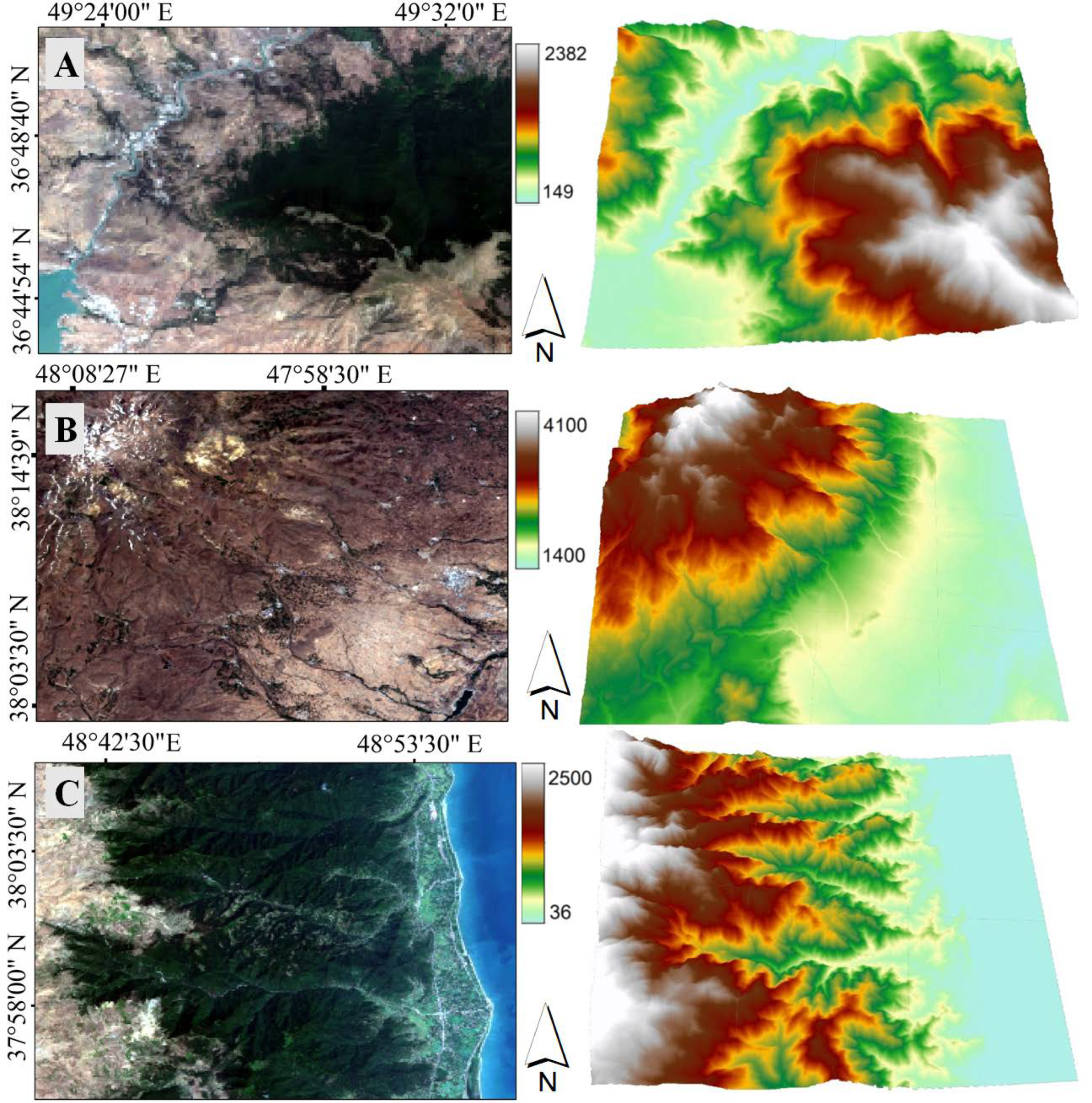
2. Study Areas
3. Method
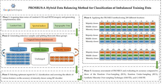
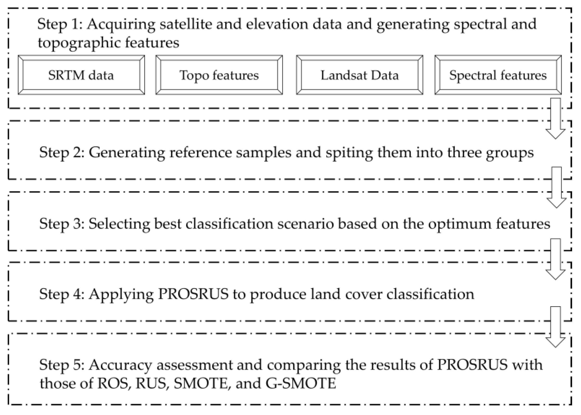
3.1. Overall Workflow
3.2. Acquiring Landsat and Elevation Data, and Generating Complementary Data within the GEE Platform
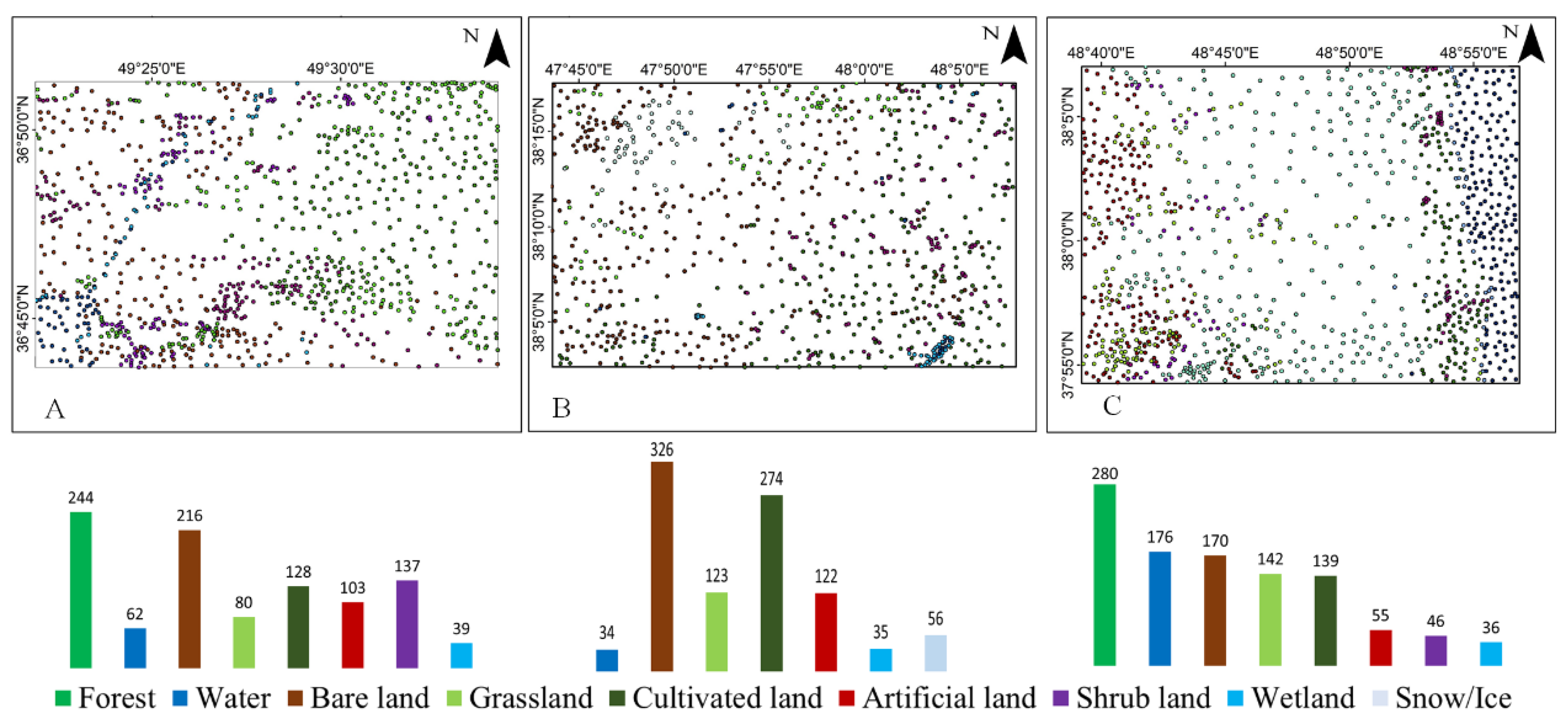
3.3. Generating Reference Samples and Spitting Them into Majority, Middle, and Minority Groups
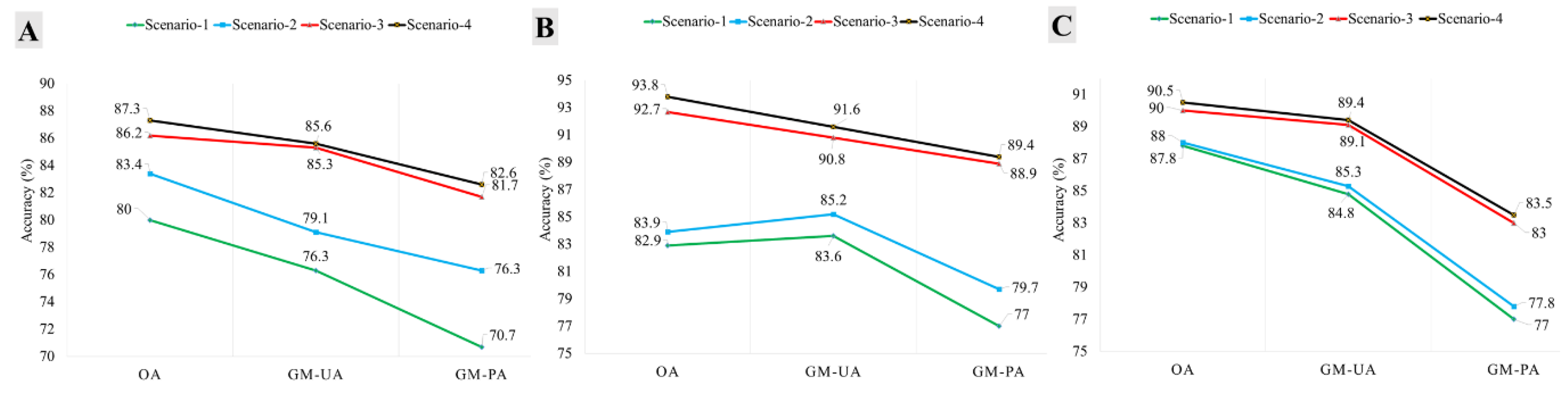
3.4. Selecting Best Classification Scenario Based on the Optimum Features
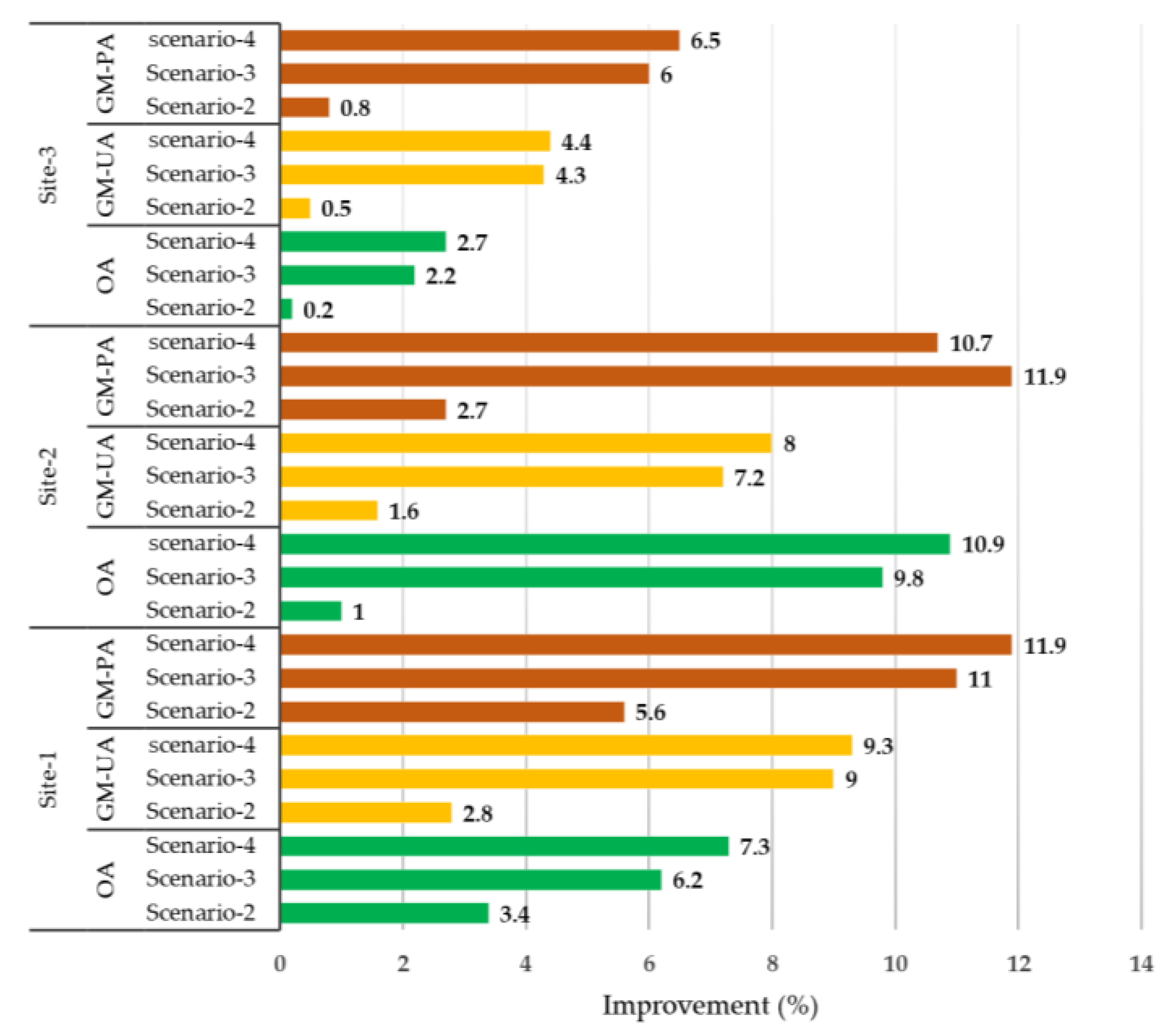
- Scenario 1: Time-series of Landsat images + original imbalanced data.
- Scenario 2: Time-series of Landsat images + spectral indices + original imbalanced data.
- Scenario 3: Time-series of Landsat images + topographic features + original imbalanced data.
- Scenario 4: Time-series of Landsat images + topographic features + spectral indices+ original imbalanced data.
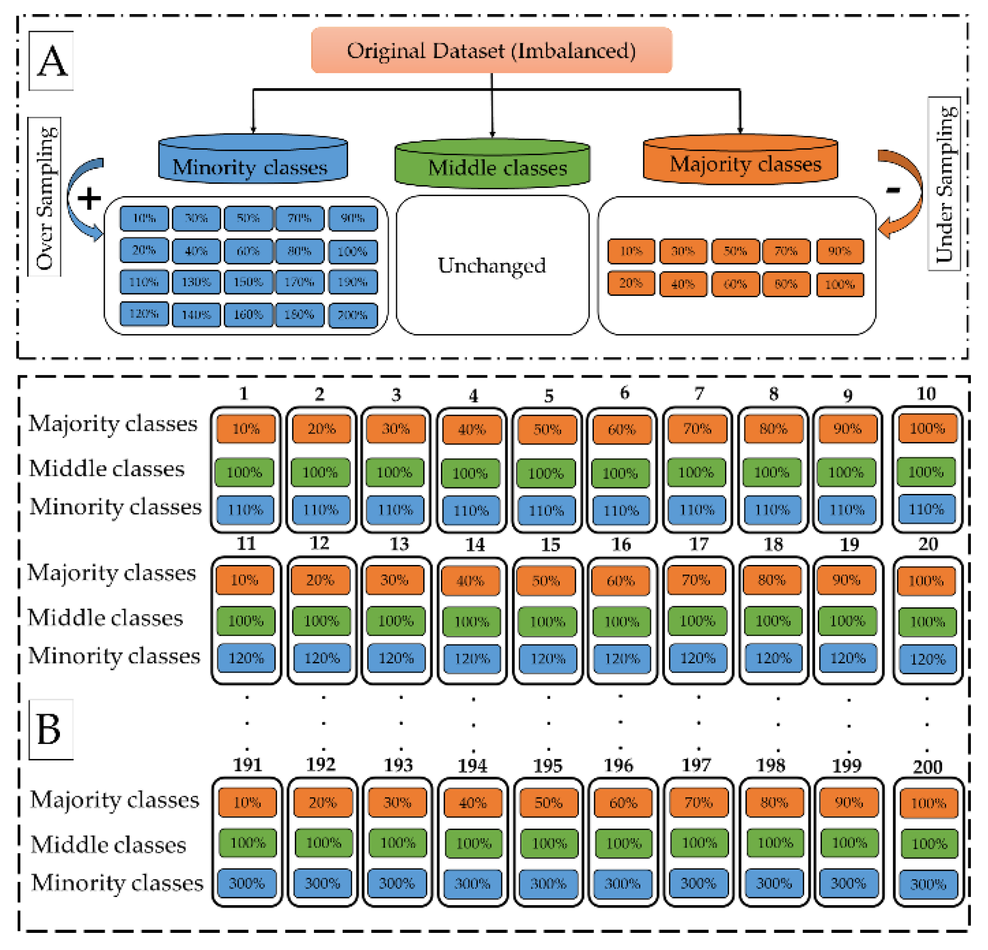
3.5. Applying PROSRUS Method
3.6. Accuracy Assessment and Comparison
4. Results
4.1. Optimum Classification Scenario
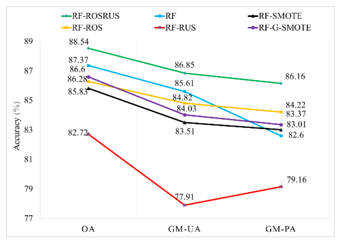
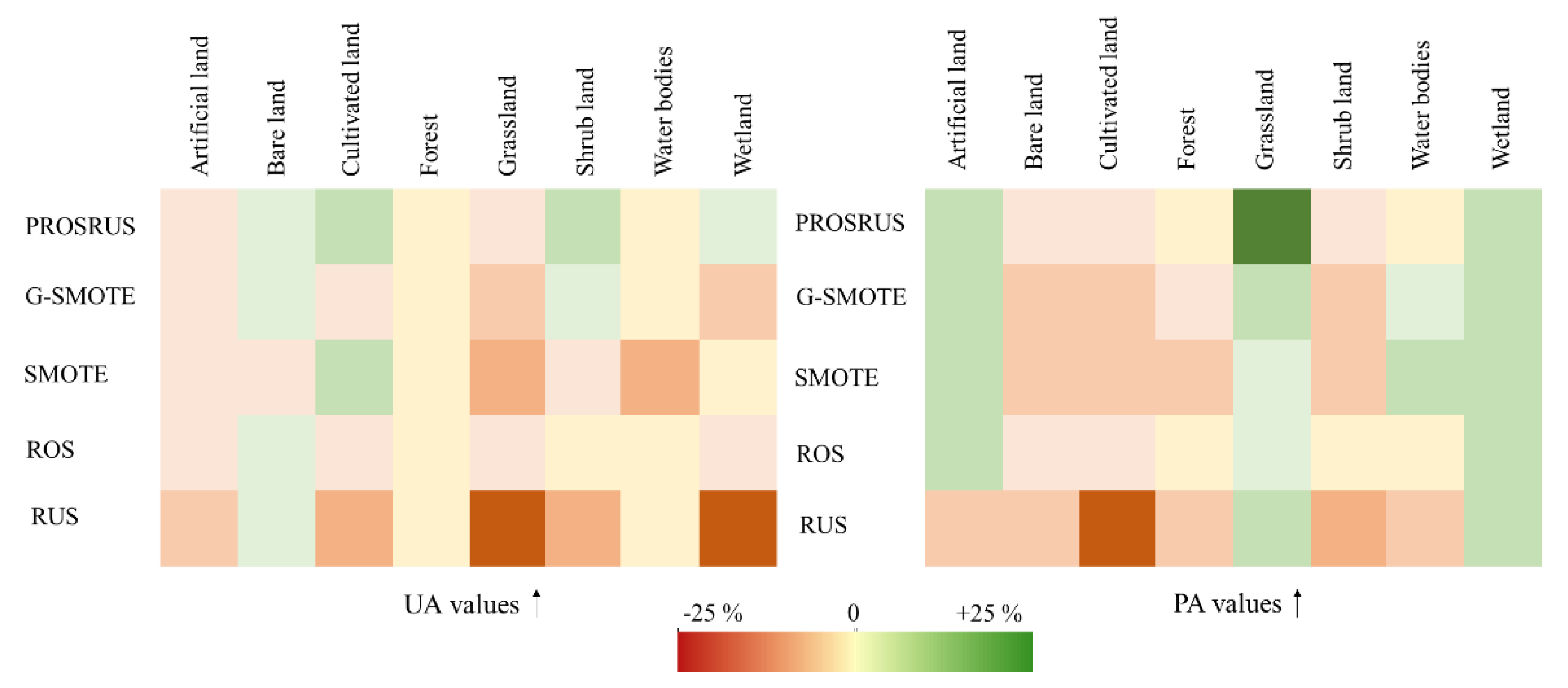
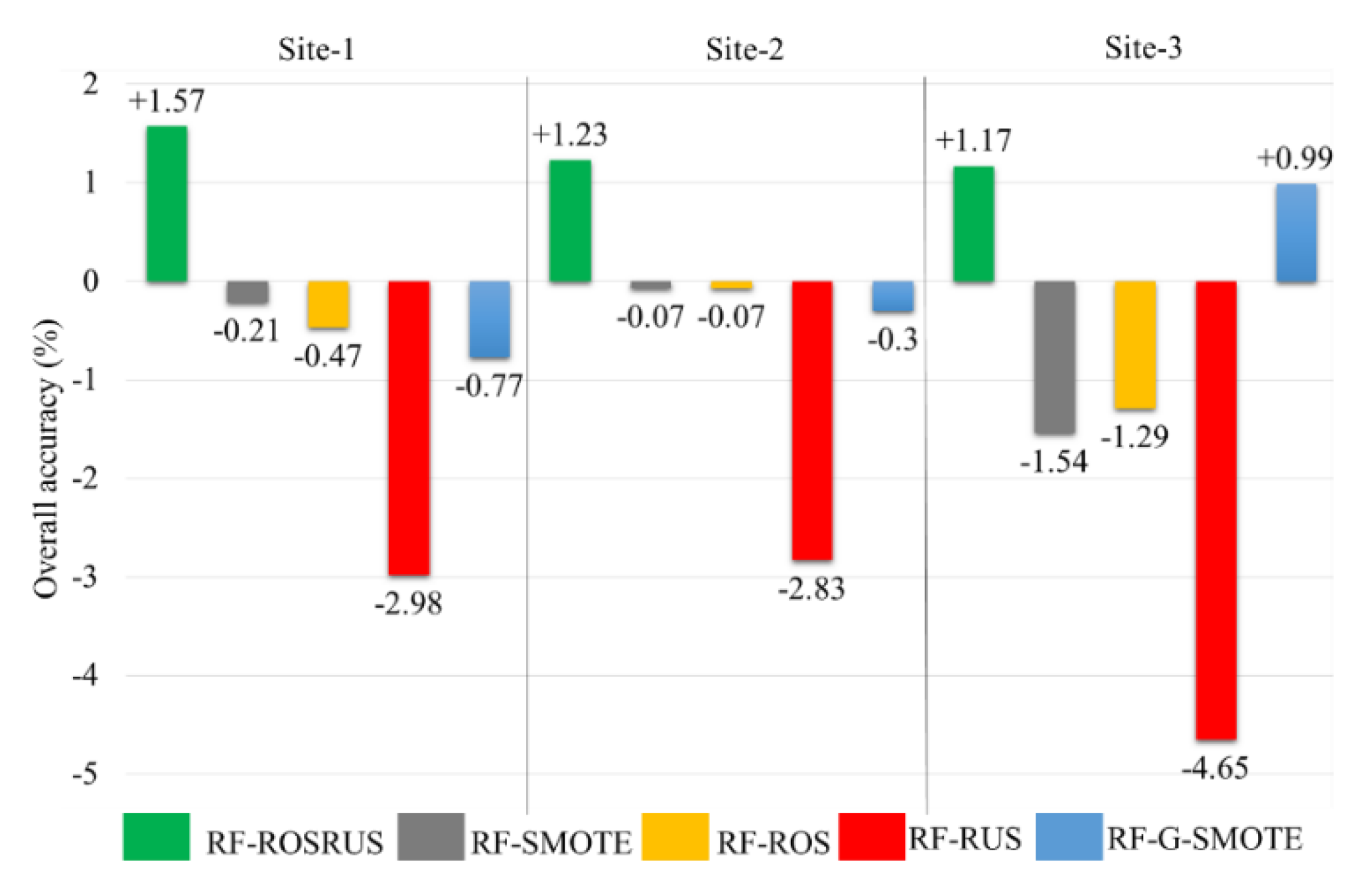
4.2. Comparison of Balancing Techniques
4.2.1. Site-1
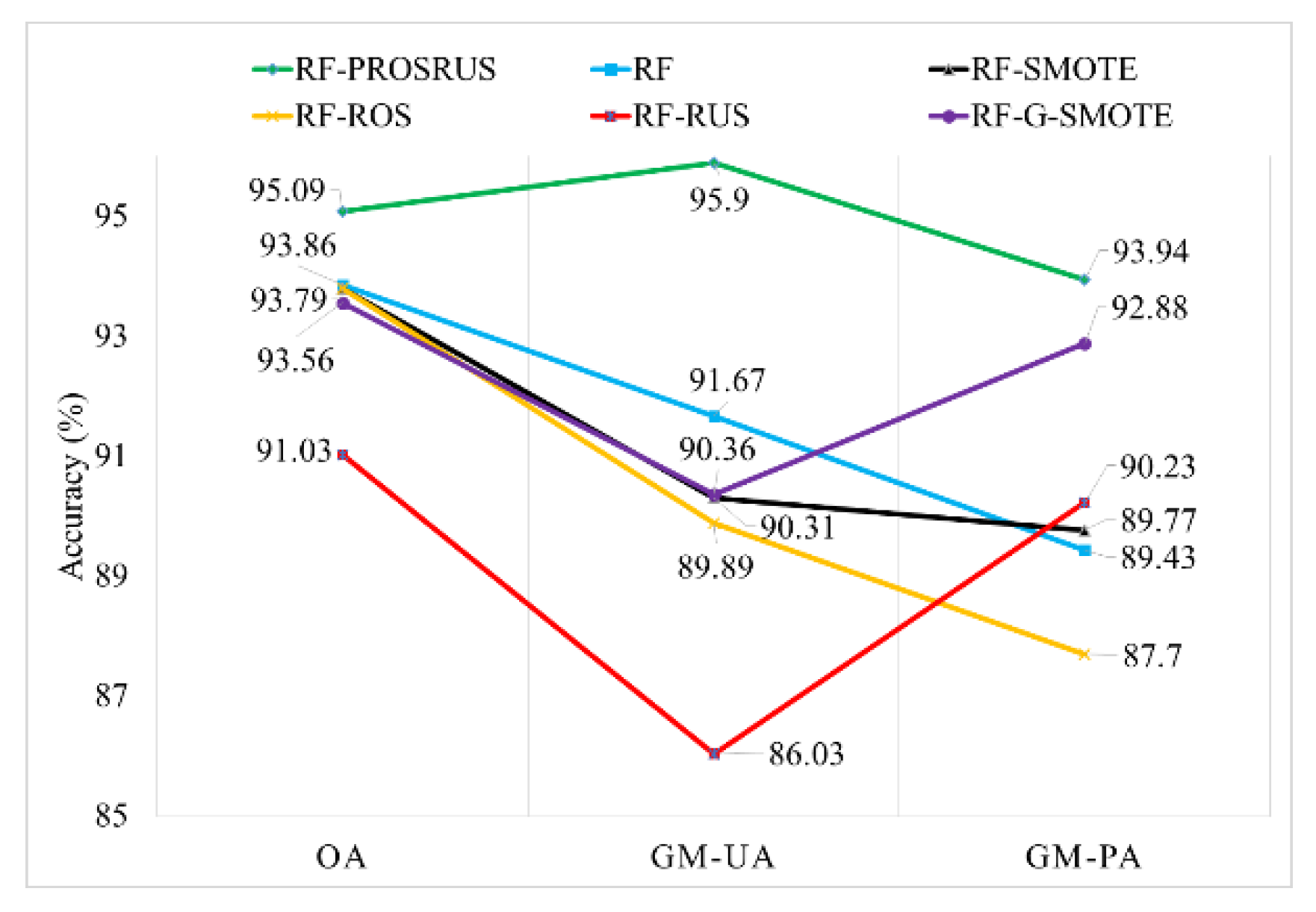
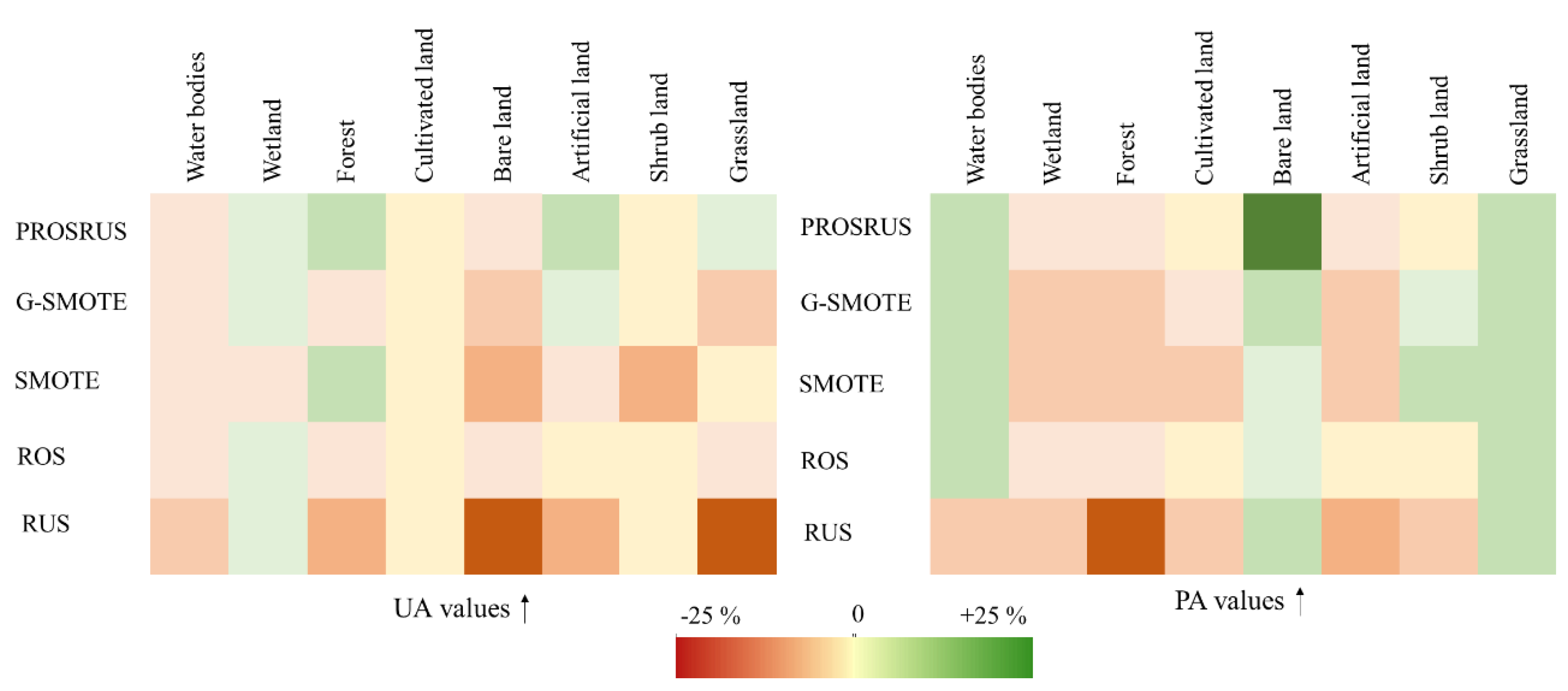
4.2.2. Site-2
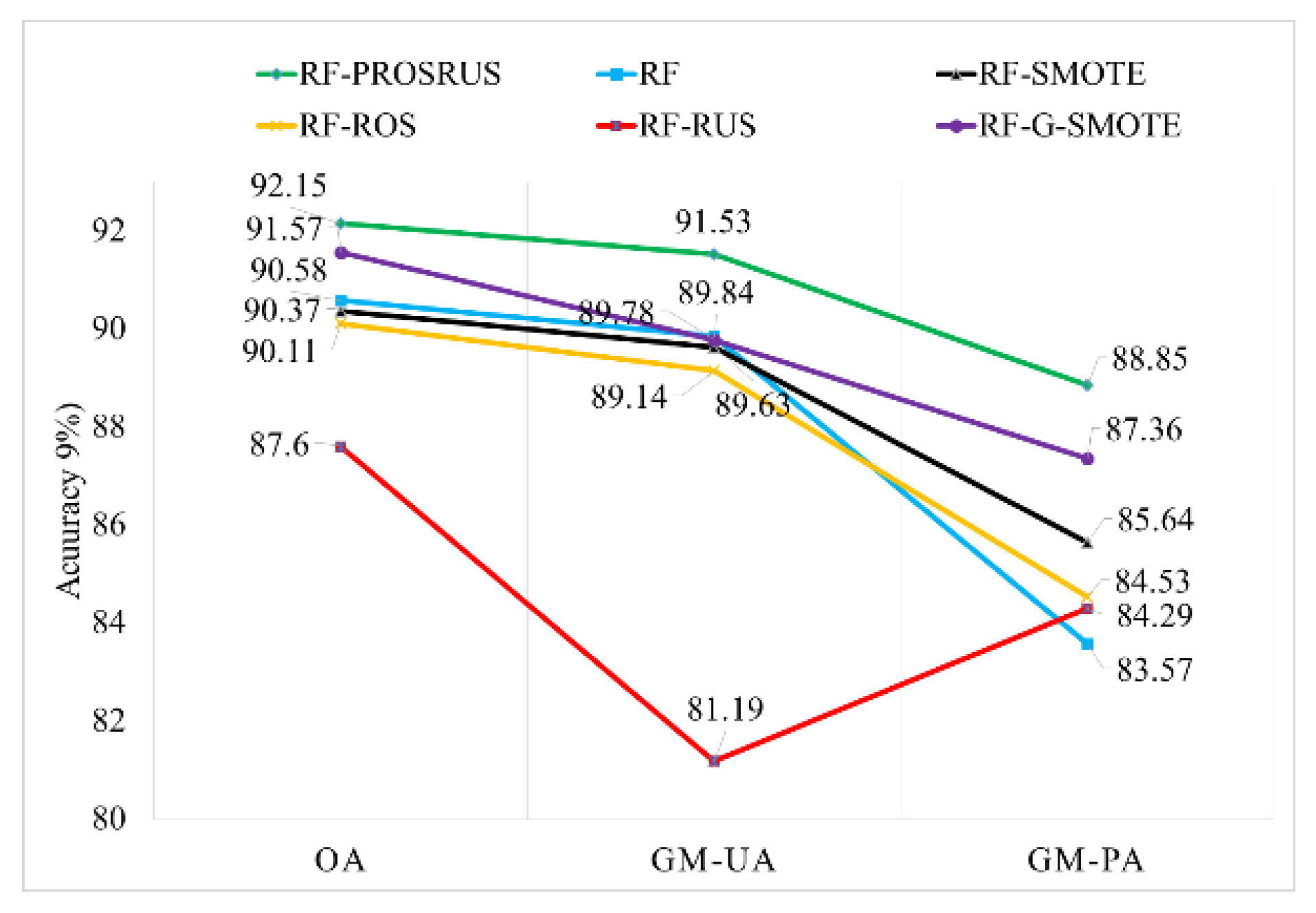
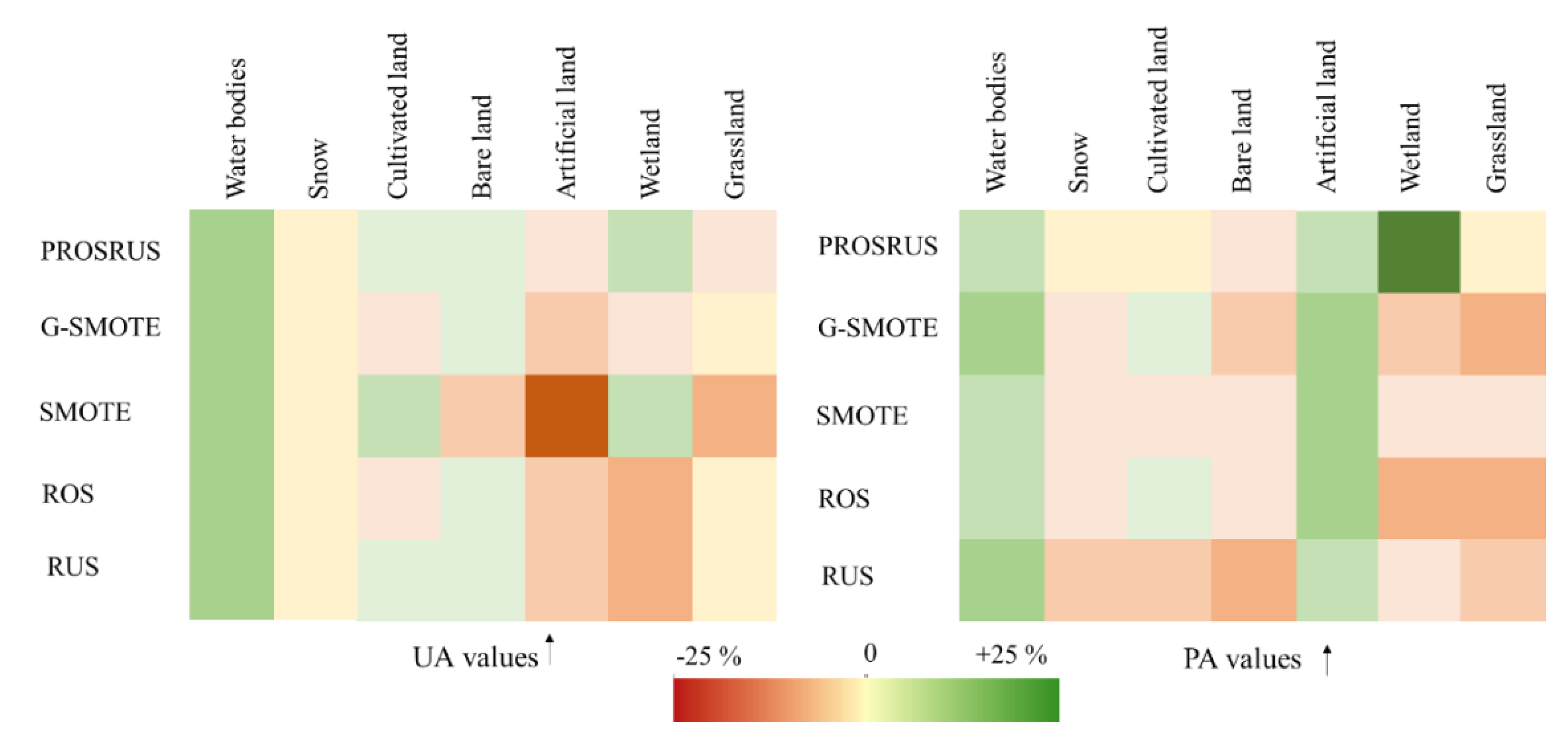
4.2.3. Site-3
5. Discussion
6. Conclusions
Supplementary Materials
Author Contributions
Funding
Conflicts of Interest
Appendix A

| ID | Site | WRS_Path | WRS_Row | Cloud Cover | Sensing Time |
|---|---|---|---|---|---|
| 1 | 1 | 166 | 34 | 5.4 | 2019-06-27 |
| 2 | 1 | 166 | 34 | 3.92 | 2019-09-15 |
| 3 | 1 | 166 | 35 | 0.9 | 2019-06-11 |
| 4 | 1 | 166 | 35 | 0.13 | 2019-06-27 |
| 5 | 1 | 166 | 35 | 0.61 | 2019-07-13 |
| 6 | 1 | 166 | 35 | 2.61 | 2019-07-29 |
| 7 | 1 | 166 | 35 | 1.08 | 2019-08-14 |
| 8 | 1 | 166 | 35 | 3.81 | 2019-08-30 |
| 9 | 1 | 166 | 35 | 0.13 | 2019-09-15 |
| 10 | 2 | 167 | 33 | 2.21 | 2019-06-18 |
| 11 | 2 | 167 | 33 | 7.94 | 2019-07-04 |
| 12 | 2 | 167 | 33 | 2.78 | 2019-07-20 |
| 13 | 2 | 167 | 33 | 6.29 | 2019-08-05 |
| 14 | 2 | 167 | 33 | 0.72 | 2019-08-21 |
| 15 | 2 | 167 | 34 | 8.7 | 2019-05-01 |
| 16 | 2 | 167 | 34 | 6.75 | 2019-05-17 |
| 17 | 2 | 167 | 34 | 1.77 | 2019-06-02 |
| 18 | 2 | 167 | 34 | 1.96 | 2019-06-18 |
| 19 | 2 | 167 | 34 | 1.96 | 2019-07-04 |
| 20 | 2 | 167 | 34 | 1.74 | 2019-07-20 |
| 21 | 2 | 167 | 34 | 2.9 | 2019-08-05 |
| 22 | 2 | 167 | 34 | 1 | 2019-08-21 |
| 23 | 3 | 167 | 34 | 5.4 | 2019-06-27 |
| 24 | 3 | 166 | 34 | 3.92 | 2019-09-15 |
| 25 | 3 | 167 | 33 | 2.21 | 2019-06-18 |
| 26 | 3 | 167 | 33 | 7.94 | 2019-07-04 |
| 27 | 3 | 167 | 33 | 2.78 | 2019-07-20 |
| 28 | 3 | 167 | 33 | 6.29 | 2019-08-05 |
| 29 | 3 | 167 | 33 | 0.72 | 2019-08-21 |
| 30 | 3 | 167 | 34 | 8.7 | 2019-05-01 |
| 31 | 3 | 167 | 34 | 6.75 | 2019-05-17 |
| 32 | 3 | 167 | 34 | 1.77 | 2019-06-02 |
| 33 | 3 | 167 | 34 | 1.96 | 2019-06-18 |
| 34 | 3 | 167 | 34 | 1.96 | 2019-07-04 |
| 35 | 3 | 167 | 34 | 1.74 | 2019-07-20 |
| 36 | 3 | 167 | 34 | 2.9 | 2019-08-05 |
| 37 | 3 | 167 | 34 | 0.98 | 2019-08-21 |
Appendix B
| Experiment Sites | Scenarios | Evaluation Metrics (per Class) | LC Classes | Overall Metrics | ||||||||||
|---|---|---|---|---|---|---|---|---|---|---|---|---|---|---|
| Artificial Land | Bare Land | Cultivated Land | Forest | Grassland | Shrub Land | Water Bodies | Wetland | Snow | OA (%) | GM-UA (%) | GM-PA (%) | |||
| Site-1 | 1 | UA (%) | 83.7 | 79.6 | 56.3 | 97.8 | 61.1 | 72.5 | 100 | 66.6 | - | 80 | 76.3 | 70.7 |
| PA (%) | 60.7 | 93.3 | 51.6 | 91.8 | 59.4 | 78.3 | 94.2 | 50 | - | |||||
| 2 | UA (%) | 84 | 81.5 | 67.3 | 97.8 | 66.6 | 76.8 | 100 | 66.6 | - | 83.4 | 79.1 | 76.3 | |
| PA (%) | 72.5 | 92.3 | 55 | 98.5 | 64.8 | 85.1 | 91.4 | 62.5 | - | |||||
| 3 | UA (%) | 79 | 78.5 | 72.5 | 97.8 | 82.7 | 89.3 | 100 | 86.6 | - | 86.2 | 85.3 | 81.7 | |
| PA (%) | 66.6 | 90.4 | 75 | 97.8 | 64.8 | 90.5 | 94.2 | 81.2 | - | |||||
| 4 | UA (%) | 85 | 83.4 | 73.5 | 97.8 | 80 | 87 | 100 | 81.2 | - | 87.3 | 85.6 | 82.6 | |
| PA (%) | 66.6 | 91.4 | 83.3 | 97.8 | 64.8 | 90.5 | 91.4 | 81.2 | - | |||||
| Site-2 | 1 | UA (%) | 88.8 | 84.7 | 79.4 | - | 71.7 | - | 80 | 83.3 | 100 | 82.9 | 83.6 | 77 |
| PA (%) | 77.7 | 91.7 | 84.5 | - | 85.9 | - | 80 | 62.5 | 90.4 | |||||
| 2 | UA (%) | 89 | 85.4 | 84.7 | - | 76 | - | 80 | 83.3 | 100 | 83.9 | 85.2 | 79.7 | |
| PA (%) | 79.1 | 89.9 | 88 | - | 62.5 | - | 80 | 68.7 | 95.2 | |||||
| 3 | UA (%) | 96.9 | 95.3 | 90.6 | - | 94.1 | - | 76.6 | 84.3 | 100 | 92.7 | 90.8 | 88.9 | |
| PA (%) | 86.8 | 96.4 | 96.4 | - | 80.7 | - | 80 | 83.5 | 100 | |||||
| 4 | UA (%) | 96.9 | 96.5 | 90.8 | - | 94.1 | - | 78.5 | 86.6 | 100 | 93.8 | 91.6 | 89.4 | |
| PA (%) | 87.5 | 97.6 | 97.8 | - | 85.7 | - | 78.5 | 81.2 | 100 | |||||
| Site-3 | 1 | UA (%) | 84.4 | 80 | 85.3 | 94.4 | 73.5 | 76.9 | 98.8 | 82.2 | - | 87.8 | 84.8 | 77 |
| PA (%) | 60.7 | 84.4 | 84.8 | 97.8 | 75.7 | 45.4 | 98.8 | 82.2 | - | |||||
| 2 | UA (%) | 85 | 82.7 | 85.5 | 94.4 | 69.3 | 83.3 | 98.8 | 86.6 | - | 88 | 85.3 | 77.8 | |
| PA (%) | 60.7 | 84.7 | 89.4 | 98.5 | 80.3 | 45.4 | 98.8 | 82.2 | - | |||||
| 3 | UA (%) | 89.3 | 87.2 | 85.1 | 94.4 | 76.1 | 84.6 | 98.8 | 100 | - | 90 | 89.1 | 83 | |
| PA (%) | 89.2 | 86.2 | 92.4 | 97.8 | 80.3 | 50 | 98.8 | 82.2 | - | |||||
| 4 | UA (%) | 89.3 | 88.1 | 88.5 | 94.4 | 77.1 | 84.6 | 98.8 | 100 | - | 90.5 | 89.4 | 83.5 | |
| PA (%) | 89.2 | 87 | 93.9 | 97.8 | 81.8 | 50 | 98.8 | 88.2 | - | |||||
Appendix C
| Method | Evaluation Metrics (per Class) | LC Classes | Overall Metrics | |||||||||
|---|---|---|---|---|---|---|---|---|---|---|---|---|
| Artificial Land | Bare Land | Cultivated Land | Forest | Grassland | Shrub Land | Water Bodies | Wetland | OA (%) | GM-UA (%) | GM-PA (%) | ||
| RF-ROSRUS-190 | UA (%) | 84.1 | 86.2 | 77.4 | 97.8 | 78.1 | 91.6 | 100 | 82.3 | 88.54 | 86.85 | 86.16 |
| PA (%) | 72.5 | 89.5 | 80 | 97.8 | 83.8 | 89.2 | 91.4 | 87.5 | ||||
| RF-Scenario 4 (original data) | UA (%) | 85 | 83.4 | 73.5 | 97.8 | 80 | 87 | 100 | 81.2 | 87.37 | 85.61 | 82.60 |
| PA (%) | 66.6 | 91.4 | 83.3 | 97.8 | 64.8 | 90.5 | 91.4 | 81.2 | ||||
| RF-SMOTE | UA (%) | 80.3 | 79 | 80 | 97.8 | 72.9 | 85.1 | 94.2 | 81.2 | 85.83 | 83.51 | 83.01 |
| PA (%) | 70.7 | 85.5 | 76.2 | 91.1 | 67.5 | 88.3 | 97 | 86.6 | ||||
| RF-ROS | UA (%) | 82.2 | 86 | 72.7 | 97.8 | 78.7 | 87 | 100 | 77.7 | 86.28 | 84.82 | 84.22 |
| PA (%) | 72.5 | 87.6 | 80 | 97.8 | 70.2 | 90.5 | 91.4 | 87.5 | ||||
| RF-RUS | UA (%) | 81 | 85.1 | 63.5 | 97.8 | 62.2 | 80 | 100 | 63.6 | 82.72 | 77.91 | 79.16 |
| PA (%) | 58.8 | 81.9 | 66.6 | 91.8 | 75.6 | 86.5 | 85.7 | 87.5 | ||||
Appendix D
| Method | Evaluation Metrics (per Class) | LC Classes | Overall Metrics | ||||||||
|---|---|---|---|---|---|---|---|---|---|---|---|
| Water Bodies | Snow | Cultivated Land | Bare Land | Artificial Land | Wetland | Grassland | OA (%) | GM-UA (%) | GM-PA (%) | ||
| RF-ROSRUS-26 | UA (%) | 100 | 100 | 91.4 | 98.2 | 95.7 | 94.1 | 92.3 | 95.09 | 95.9 | 93.94 |
| PA (%) | 85.7 | 100 | 97.8 | 96.5 | 93.1 | 100 | 85.7 | ||||
| RF-Scenario 4 (original data) | UA (%) | 78.5 | 100 | 90.8 | 96.5 | 96.9 | 86.6 | 94.1 | 93.86 | 91.67 | 89.43 |
| PA (%) | 78.5 | 100 | 97.8 | 97.6 | 87.5 | 81.2 | 85.7 | ||||
| RF-SMOTE | UA (%) | 88.8 | 100 | 97.3 | 89.8 | 73.3 | 91.4 | 84.2 | 93.79 | 90.31 | 89.77 |
| PA (%) | 84.2 | 96 | 97 | 94.7 | 98.1 | 78.5 | 82 | ||||
| RF-ROS | UA (%) | 88.8 | 100 | 90.4 | 98 | 91.4 | 76.9 | 100 | 93.79 | 91.89 | 87.70 |
| PA (%) | 84.2 | 96 | 100 | 94.7 | 98.1 | 71.4 | 74.3 | ||||
| RF-RUS | UA (%) | 90 | 100 | 93.2 | 97.8 | 91.3 | 76.9 | 100 | 91.03 | 86.03 | 90.23 |
| PA (%) | 94.7 | 96 | 93.9 | 88.1 | 94.4 | 78.5 | 78.1 | ||||
Appendix E
| Method |
Evaluation Metrics (per Class) | LC Classes | Overall Metrics | ||||||||
|---|---|---|---|---|---|---|---|---|---|---|---|
| Water Bodies | Snow | Cultivated Land | Bare Land | Artificial Land | Wetland | Grassland | OA (%) | GM-UA (%) | GM-PA (%) | ||
| RF-ROSRUS-26 | UA (%) | 100 | 100 | 91.4 | 98.2 | 95.7 | 94.1 | 92.3 | 95.09 | 95.9 | 93.94 |
| PA (%) | 85.7 | 100 | 97.8 | 96.5 | 93.1 | 100 | 85.7 | ||||
| RF-Scenario 4 (original data) | UA (%) | 78.5 | 100 | 90.8 | 96.5 | 96.9 | 86.6 | 94.1 | 93.86 | 91.67 | 89.43 |
| PA (%) | 78.5 | 100 | 97.8 | 97.6 | 87.5 | 81.2 | 85.7 | ||||
| RF-SMOTE | UA (%) | 88.8 | 100 | 97.3 | 89.8 | 73.3 | 91.4 | 84.2 | 93.79 | 90.31 | 89.77 |
| PA (%) | 84.2 | 96 | 97 | 94.7 | 98.1 | 78.5 | 82 | ||||
| RF-ROS | UA (%) | 88.8 | 100 | 90.4 | 98 | 91.4 | 76.9 | 100 | 93.79 | 91.89 | 87.70 |
| PA (%) | 84.2 | 96 | 100 | 94.7 | 98.1 | 71.4 | 74.3 | ||||
| RF-RUS | UA (%) | 90 | 100 | 93.2 | 97.8 | 91.3 | 76.9 | 100 | 91.03 | 86.03 | 90.23 |
| PA (%) | 94.7 | 96 | 93.9 | 88.1 | 94.4 | 78.5 | 78.1 | ||||
References
- Friend, D.A. Mountain geography in 2002: The international year of mountains. Geogr. Rev. 2002, 92, iii–vi. [Google Scholar] [CrossRef]
- Bian, J.; Li, A.; Lei, G.; Zhang, Z.; Nan, X. Global high-resolution mountain green cover index mapping based on landsat images and google earth engine. ISPRS J. Photogramm. Remote Sens. 2020, 162, 63–76. [Google Scholar] [CrossRef]
- Chu, D. Remote Sensing of Land Use and Land Cover in Mountain Region; Springer: New York, NY, USA, 2020. [Google Scholar]
- Adepoju, K.; Adelabu, S. Improved landsat-8 OLI and sentinel-2 MSI classification in mountainous terrain using machine learning on google earth engine. In Proceedings of the Biennial Conference of the Society of South African Geographers, Bloemfontein, South Africa, 1–5 October 2018; p. 5. [Google Scholar]
- Ghorbanzadeh, O.; Valizadeh Kamran, K.; Blaschke, T.; Aryal, J.; Naboureh, A.; Einali, J.; Bian, J. Spatial prediction of wildfire susceptibility using field survey GPS data and machine learning approaches. Fire 2019, 2, 43. [Google Scholar] [CrossRef] [Green Version]
- Moharrami, M.; Naboureh, A.; Gudiyangada Nachappa, T.; Ghorbanzadeh, O.; Guan, X.; Blaschke, T. National-scale landslide susceptibility mapping in Austria using fuzzy best-worst multi-criteria decision-making. ISPRS Int. J. Geo-Inf. 2020, 9, 393. [Google Scholar] [CrossRef]
- Ghorbanzadeh, O.; Blaschke, T.; Gholamnia, K.; Aryal, J. Forest fire susceptibility and risk mapping using social/infrastructural vulnerability and environmental variables. Fire 2019, 2, 50. [Google Scholar] [CrossRef] [Green Version]
- Amani, M.; Salehi, B.; Mahdavi, S.; Granger, J.E.; Brisco, B.; Hanson, A. Wetland classification using multi-source and multi-temporal optical remote sensing data in newfoundland and Labrador, Canada. Can. J. Remote Sens. 2017, 43, 360–373. [Google Scholar] [CrossRef]
- Lei, G.; Li, A.; Bian, J.; Zhang, Z.; Jin, H.; Xi, N.; Wei, Z.; Wang, J.; Cao, X.; Tan, J. Land cover mapping in southwestern china using the HC-MMK approach. Remote Sens. 2016, 8, 305. [Google Scholar] [CrossRef] [Green Version]
- Mahdavi, S.; Salehi, B.; Amani, M.; Granger, J.E.; Brisco, B.; Huang, W.; Hanson, A. Object-based classification of wetlands in Newfoundland and Labrador using multi-temporal PolSAR data. Can. J. Remote Sens. 2017, 43, 432–450. [Google Scholar] [CrossRef]
- Rodríguez-Jeangros, N.; Hering, A.S.; Kaiser, T.; McCray, J.E. ScaMF–RM: A fused high-resolution land cover product of the Rocky Mountains. Remote Sens. 2017, 9, 1015. [Google Scholar] [CrossRef] [Green Version]
- Kan, X.; Zhang, Y.; Zhu, L.; Xiao, L.; Wang, J.; Tian, W.; Tan, H. Snow cover mapping for mountainous areas by fusion of MODIS L1B and geographic data based on stacked denoising auto-encoders. Comput. Mater. Contin. 2018, 57, 49–68. [Google Scholar] [CrossRef]
- Liu, C.; Huang, X.; Li, X.; Liang, T. MODIS fractional snow cover mapping using machine learning technology in a mountainous area. Remote Sens. 2020, 12, 962. [Google Scholar] [CrossRef] [Green Version]
- Lei, G.; Li, A.; Bian, J.; Yan, H.; Zhang, L.; Zhang, Z.; Nan, X. OIC-MCE: A practical land cover mapping approach for limited samples based on multiple classifier ensemble and iterative classification. Remote Sens. 2020, 12, 987. [Google Scholar] [CrossRef] [Green Version]
- Delalay, M.; Tiwari, V.; Ziegler, A.D.; Gopal, V.; Passy, P. Land-use and land-cover classification using sentinel-2 data and machine-learning algorithms: Operational method and its implementation for a mountainous area of Nepal. J. Appl. Remote Sens. 2019, 13, 014530. [Google Scholar] [CrossRef]
- Galar, M.; Fernandez, A.; Barrenechea, E.; Bustince, H.; Herrera, F. A review on ensembles for the class imbalance problem: Bagging-, boosting-, and hybrid-based approaches. IEEE Trans. Syst. Man Cybern. Part C Appl. Rev. 2012, 42, 463–484. [Google Scholar] [CrossRef]
- Mellor, A.; Boukir, S.; Haywood, A.; Jones, S. Exploring issues of training data imbalance and mislabelling on random forest performance for large area land cover classification using the ensemble margin. ISPRS J. Photogramm. Remote Sens. 2015, 105, 155–168. [Google Scholar] [CrossRef]
- Azadbakht, M.; Fraser, C.S.; Khoshelham, K. Synergy of sampling techniques and ensemble classifiers for classification of urban environments using full-waveform LidAR data. Int. J. Appl. Earth Obs. Geoinf. 2018, 73, 277–291. [Google Scholar] [CrossRef]
- Feng, W.; Dauphin, G.; Huang, W.; Quan, Y.; Bao, W.; Wu, M.; Li, Q. Dynamic synthetic minority over-sampling technique-based rotation forest for the classification of imbalanced hyperspectral data. IEEE J. Sel. Top. Appl. Earth Obs. Remote Sens. 2019, 12, 2159–2169. [Google Scholar] [CrossRef]
- Liu, X.-Y.; Zhou, Z.-H. The influence of class imbalance on cost-sensitive learning: An empirical study. In Proceedings of the Sixth International Conference on Data Mining (ICDM’06), Hong Kong, China, 18–22 December 2006; IEEE: New York, NY, USA, 2006; pp. 970–974. [Google Scholar]
- Chawla, N.V.; Bowyer, K.W.; Hall, L.O.; Kegelmeyer, W.P. Smote: Synthetic minority over-sampling technique. J. Artif. Intell. Res. 2002, 16, 321–357. [Google Scholar] [CrossRef]
- Khan, S.H.; Hayat, M.; Bennamoun, M.; Sohel, F.A.; Togneri, R. Cost-sensitive learning of deep feature representations from imbalanced data. IEEE Trans. Neural Netw. Learn. Syst. 2017, 29, 3573–3587. [Google Scholar]
- Haixiang, G.; Yijing, L.; Shang, J.; Mingyun, G.; Yuanyue, H.; Bing, G. Learning from class-imbalanced data: Review of methods and applications. Expert Syst. Appl. 2017, 73, 220–239. [Google Scholar] [CrossRef]
- Chawla, N.V. Data mining for imbalanced datasets: An overview. In Data Mining and Knowledge Discovery Handbook; Springer: New York, NY, USA, 2009; pp. 875–886. [Google Scholar]
- Waldner, F.; Chen, Y.; Lawes, R.; Hochman, Z. Needle in a haystack: Mapping rare and infrequent crops using satellite imagery and data balancing methods. Remote Sens. Environ. 2019, 233, 111375. [Google Scholar] [CrossRef]
- Feng, W.; Boukir, S.; Huang, W. Margin-based random forest for imbalanced land cover classification. In Proceedings of the IGARSS 2019—2019 IEEE International Geoscience and Remote Sensing Symposium, Yokohama, Japan, 28 June–2 August 2019; IEEE: New York, NY, USA, 2019; pp. 3085–3088. [Google Scholar]
- Douzas, G.; Bacao, F.; Fonseca, J.; Khudinyan, M. Imbalanced learning in land cover classification: Improving minority classes’ prediction accuracy using the geometric smote algorithm. Remote Sens. 2019, 11, 3040. [Google Scholar] [CrossRef] [Green Version]
- Bogner, C.; Seo, B.; Rohner, D.; Reineking, B. Classification of rare land cover types: Distinguishing annual and perennial crops in an agricultural catchment in South Korea. PLoS ONE 2018, 13, e0190476. [Google Scholar] [CrossRef] [PubMed] [Green Version]
- Hurskainen, P.; Adhikari, H.; Siljander, M.; Pellikka, P.; Hemp, A. Auxiliary datasets improve accuracy of object-based land use/land cover classification in heterogeneous savanna landscapes. Remote Sens. Environ. 2019, 233, 111354. [Google Scholar] [CrossRef]
- Xie, S.; Liu, L.; Zhang, X.; Yang, J.; Chen, X.; Gao, Y. Automatic land-cover mapping using Landsat time-series data based on google earth engine. Remote Sens. 2019, 11, 3023. [Google Scholar] [CrossRef] [Green Version]
- Hermosilla, T.; Wulder, M.A.; White, J.C.; Coops, N.C.; Hobart, G.W. Regional detection, characterization, and attribution of annual forest change from 1984 to 2012 using Landsat-derived time-series metrics. Remote Sens. Environ. 2015, 170, 121–132. [Google Scholar] [CrossRef]
- Gorelick, N.; Hancher, M.; Dixon, M.; Ilyushchenko, S.; Thau, D.; Moore, R. Google earth engine: Planetary-scale geospatial analysis for everyone. Remote Sens. Environ. 2017, 202, 18–27. [Google Scholar] [CrossRef]
- Eskandari, S.; Reza Jaafari, M.; Oliva, P.; Ghorbanzadeh, O.; Blaschke, T. Mapping land cover and tree canopy cover in Zagros forests of Iran: Application of sentinel-2, google earth, and field data. Remote Sens. 2020, 12, 1912. [Google Scholar] [CrossRef]
- Amani, M.; Brisco, B.; Afshar, M.; Mirmazloumi, S.M.; Mahdavi, S.; Mirzadeh, S.M.J.; Huang, W.; Granger, J. A generalized supervised classification scheme to produce provincial wetland inventory maps: An application of google earth engine for big geo data processing. Big Earth Data 2019, 3, 378–394. [Google Scholar] [CrossRef]
- Amani, M.; Mahdavi, S.; Afshar, M.; Brisco, B.; Huang, W.; Mohammad Javad Mirzadeh, S.; White, L.; Banks, S.; Montgomery, J.; Hopkinson, C. Canadian wetland inventory using google earth engine: The first map and preliminary results. Remote Sens. 2019, 11, 842. [Google Scholar] [CrossRef] [Green Version]
- Raziei, T. Koppen-Geiger climate classification of Iran and investigation of its changes during 20th century. J. Earth Space Phys. 2017, 43, 419–439. [Google Scholar]
- Batista, G.E.; Prati, R.C.; Monard, M.C. A study of the behavior of several methods for balancing machine learning training data. ACM SIGKDD Explor. Newsl. 2004, 6, 20–29. [Google Scholar] [CrossRef]
- Douzas, G.; Bacao, F. Geometric smote a geometrically enhanced drop-in replacement for smote. Inf. Sci. 2019, 501, 118–135. [Google Scholar] [CrossRef]
- Ghorbanian, A.; Kakooei, M.; Amani, M.; Mahdavi, S.; Mohammadzadeh, A.; Hasanlou, M. Improved land cover map of Iran using sentinel imagery within google earth engine and a novel automatic workflow for land cover classification using migrated training samples. ISPRS J. Photogramm. Remote Sens. 2020, 167, 276–288. [Google Scholar] [CrossRef]
- Naboureh, A.; Moghaddam, M.H.R.; Feizizadeh, B.; Blaschke, T. An integrated object-based image analysis and CA-Markov model approach for modeling land use/land cover trends in the Sarab plain. Arab. J. Geosci. 2017, 10, 259. [Google Scholar] [CrossRef]
- Zha, Y.; Gao, J.; Ni, S. Use of normalized difference built-up index in automatically mapping urban areas from tm imagery. Int. J. Remote Sens. 2003, 24, 583–594. [Google Scholar] [CrossRef]
- Yang, X.; Zhao, S.; Qin, X.; Zhao, N.; Liang, L. Mapping of urban surface water bodies from sentinel-2 MSI imagery at 10 m resolution via NDWI-based image sharpening. Remote Sens. 2017, 9, 596. [Google Scholar] [CrossRef] [Green Version]
- Huete, A. A soil-adjusted vegetation index (SAVI). Remote Sens. Environ. 1988, 25, 295–309. [Google Scholar] [CrossRef]
- Rouse, J.; Haas, R.; Schell, J.; Deering, D. Monitoring vegetation systems in the Great Plains with ERTS. NASA Spec. Publ. 1974, 351, 309. [Google Scholar]
- McFeeters, S.K. The use of the normalized difference water index (NDWI) in the delineation of open water features. Int. J. Remote Sens. 1996, 17, 1425–1432. [Google Scholar] [CrossRef]
- Cord, A.; Conrad, C.; Schmidt, M.; Dech, S. Standardized FAO-LCCS land cover mapping in heterogeneous tree savannas of West Africa. J. Arid Environ. 2010, 74, 1083–1091. [Google Scholar] [CrossRef]
- Ghimire, B.; Rogan, J.; Miller, J. Contextual land-cover classification: Incorporating spatial dependence in land-cover classification models using random forests and the Getis statistic. Remote Sens. Lett. 2010, 1, 45–54. [Google Scholar] [CrossRef] [Green Version]
- Pelletier, C.; Valero, S.; Inglada, J.; Champion, N.; Dedieu, G. Assessing the robustness of random forests to map land cover with high resolution satellite image time series over large areas. Remote Sens. Environ. 2016, 187, 156–168. [Google Scholar] [CrossRef]
- Phiri, D.; Morgenroth, J.; Xu, C.; Hermosilla, T. Effects of pre-processing methods on Landsat oli-8 land cover classification using obia and random forests classifier. Int. J. Appl. Earth Obs. Geoinf. 2018, 73, 170–178. [Google Scholar] [CrossRef]
- Belgiu, M.; Drăguţ, L. Random forest in remote sensing: A review of applications and future directions. ISPRS J. Photogramm. Remote Sens. 2016, 114, 24–31. [Google Scholar] [CrossRef]
- Breiman, L. Random forests. Mach. Learn. 2001, 45, 5–32. [Google Scholar] [CrossRef] [Green Version]
- Santos, M.S.; Soares, J.P.; Abreu, P.H.; Araujo, H.; Santos, J. Cross-validation for imbalanced datasets: Avoiding overoptimistic and overfitting approaches [research frontier]. IEEE Comput. Intell. Mag. 2018, 13, 59–76. [Google Scholar] [CrossRef]
- Congalton, R.G. A review of assessing the accuracy of classifications of remotely sensed data. Remote Sens. Environ. 1991, 37, 35–46. [Google Scholar] [CrossRef]
- Huang, H.; Chen, Y.; Clinton, N.; Wang, J.; Wang, X.; Liu, C.; Gong, P.; Yang, J.; Bai, Y.; Zheng, Y. Mapping major land cover dynamics in Beijing using all Landsat images in google earth engine. Remote Sens. Environ. 2017, 202, 166–176. [Google Scholar] [CrossRef]
- Carrasco, L.; O’Neil, A.W.; Morton, R.D.; Rowland, C.S. Evaluating combinations of temporally aggregated sentinel-1, sentinel-2 and Landsat 8 for land cover mapping with google earth engine. Remote Sens. 2019, 11, 288. [Google Scholar] [CrossRef] [Green Version]
- Gbodjo, Y.J.E.; Ienco, D.; Leroux, L. Toward spatio–spectral analysis of sentinel-2 time series data for land cover mapping. IEEE Geosci. Remote Sens. Lett. 2019, 17, 307–311. [Google Scholar] [CrossRef]
- Stromann, O.; Nascetti, A.; Yousif, O.; Ban, Y. Dimensionality reduction and feature selection for object-based land cover classification based on sentinel-1 and sentinel-2 time series using google earth engine. Remote Sens. 2020, 12, 76. [Google Scholar] [CrossRef] [Green Version]
- Tsai, Y.H.; Stow, D.; Chen, H.L.; Lewison, R.; An, L.; Shi, L. Mapping vegetation and land use types in Fanjingshan national nature reserve using google earth engine. Remote Sens. 2018, 10, 927. [Google Scholar] [CrossRef] [Green Version]
- Zhu, Z.; Gallant, A.L.; Woodcock, C.E.; Pengra, B.; Olofsson, P.; Loveland, T.R.; Jin, S.; Dahal, D.; Yang, L.; Auch, R.F. Optimizing selection of training and auxiliary data for operational land cover classification for the lcmap initiative. ISPRS J. Photogramm. Remote Sens. 2016, 122, 206–221. [Google Scholar] [CrossRef] [Green Version]
- Choi, J.M. A selective sampling method for imbalanced data learning on support vector machines. Grad. Theses Diss. 2010. [Google Scholar] [CrossRef] [Green Version]
- Johnson, J.M.; Khoshgoftaar, T.M. Deep learning and data sampling with imbalanced big data. In Proceedings of the 2019 IEEE 20th International Conference on Information Reuse and Integration for Data Science (IRI), Los Angeles, CA, USA, 30 July–1 August 2019; IEEE: New York, NY, USA, 2019; pp. 175–183. [Google Scholar]


| Name | Formula | Reference |
|---|---|---|
| NDVI | (NIR − Red)/(NIR + Red) | [44] |
| NDWI | (Green − NIR)/(Green + NIR) | [45] |
| SAVI | ((NIR − Red)/(NIR + Red+ L)) × (1 + L) | [43] |
| NDBI | (SWIR − NIR)/(SWIR + NIR) | [41] |
| Site | Group-1 (Minority Classes) | Group-2 (Middle Classes) | Group-3 (Majority Classes) |
|---|---|---|---|
| 1 | Wetland, Water bodies, Grassland | Shrubland, Cultivated land, Artificial land | Forest, Bare land |
| 2 | Water bodies, Snow, Wetland | Artificial land, Grassland | Cultivated land, Bare land |
| 3 | Artificial land, Shrubland, Wetland | Water bodies, Bare land, Grassland, Cultivated land | Forest |
| Sites | Evaluation Metrics (per Class) | LC Classes | ||||||||
|---|---|---|---|---|---|---|---|---|---|---|
| Artificial Land | Bare Land | Cultivated Land | Forest | Grassland | Shrub Land | Water Bodies | Wetland | Snow | ||
| Site-1 | UA (%) | +1.3 | +3.8 | +17.2 | 0 | +18.9 | +14.5 | 0 | +14.6 | none |
| PA (%) | +5.9 | −1.9 | +28.9 | +6 | +5.4 | +12.2 | 0 | +31.2% | none | |
| Site-2 | UA (%) | +8.1 | +11.8 | +9.9 | none | +22.4 | none | 0 | +3.3 | 0 |
| PA (%) | +9.8 | +5.9 | +11.8 | none | −0.2 | none | 0 | +18.7 | +9.6 | |
| Site-3 | UA (%) | +4.9 | +8.1 | +3.2 | 0 | +3.6 | +7.7 | 0 | +17.8 | none |
| PA (%) | +28.5 | +2.6 | +9.1 | 0 | +6.1 | +4.6 | 0 | +6 | none | |
© 2020 by the authors. Licensee MDPI, Basel, Switzerland. This article is an open access article distributed under the terms and conditions of the Creative Commons Attribution (CC BY) license (http://creativecommons.org/licenses/by/4.0/).
Share and Cite
Naboureh, A.; Li, A.; Bian, J.; Lei, G.; Amani, M. A Hybrid Data Balancing Method for Classification of Imbalanced Training Data within Google Earth Engine: Case Studies from Mountainous Regions. Remote Sens. 2020, 12, 3301. https://0-doi-org.brum.beds.ac.uk/10.3390/rs12203301
Naboureh A, Li A, Bian J, Lei G, Amani M. A Hybrid Data Balancing Method for Classification of Imbalanced Training Data within Google Earth Engine: Case Studies from Mountainous Regions. Remote Sensing. 2020; 12(20):3301. https://0-doi-org.brum.beds.ac.uk/10.3390/rs12203301
Chicago/Turabian StyleNaboureh, Amin, Ainong Li, Jinhu Bian, Guangbin Lei, and Meisam Amani. 2020. "A Hybrid Data Balancing Method for Classification of Imbalanced Training Data within Google Earth Engine: Case Studies from Mountainous Regions" Remote Sensing 12, no. 20: 3301. https://0-doi-org.brum.beds.ac.uk/10.3390/rs12203301