Comparison of Backpack, Handheld, Under-Canopy UAV, and Above-Canopy UAV Laser Scanning for Field Reference Data Collection in Boreal Forests

Abstract

In this work, we compared six emerging mobile laser scanning (MLS) technologies for field reference data collection at the individual tree level in boreal forest conditions. The systems under study were an in-house developed AKHKA-R3 backpack laser scanner, a handheld Zeb-Horizon laser scanner, an under-canopy UAV (Unmanned Aircraft Vehicle) laser scanning system, and three above-canopy UAV laser scanning systems providing point clouds with varying point densities. To assess the performance of the methods for automated measurements of diameter at breast height (DBH), stem curve, tree height and stem volume, we utilized all of the six systems to collect point cloud data on two 32 m-by-32 m test sites classified as sparse (n = 42 trees) and obstructed (n = 43 trees). To analyze the data collected with the two ground-based MLS systems and the under-canopy UAV system, we used a workflow based on our recent work featuring simultaneous localization and mapping (SLAM) technology, a stem arc detection algorithm, and an iterative arc matching algorithm. This workflow enabled us to obtain accurate stem diameter estimates from the point cloud data despite a small but relevant time-dependent drift in the SLAM-corrected trajectory of the scanner. We found out that the ground-based MLS systems and the under-canopy UAV system could be used to measure the stem diameter (DBH) with a root mean square error (RMSE) of 2–8%, whereas the stem curve measurements had an RMSE of 2–15% that depended on the system and the measurement height. Furthermore, the backpack and handheld scanners could be employed for sufficiently accurate tree height measurements (RMSE = 2–10%) in order to estimate the stem volumes of individual trees with an RMSE of approximately 10%. A similar accuracy was obtained when combining stem curves estimated with the under-canopy UAV system and tree heights extracted with an above-canopy flying laser scanning unit. Importantly, the volume estimation error of these three MLS systems was found to be of the same level as the error corresponding to manual field measurements on the two test sites. To analyze point cloud data collected with the three above-canopy flying UAV systems, we used a random forest model trained on field reference data collected from nearby plots. Using the random forest model, we were able to estimate the DBH of individual trees with an RMSE of 10–20%, the tree height with an RMSE of 2–8%, and the stem volume with an RMSE of 20–50%. Our results indicate that ground-based and under-canopy MLS systems provide a promising approach for field reference data collection at the individual tree level, whereas the accuracy of above-canopy UAV laser scanning systems is not yet sufficient for predicting stem attributes of individual trees for field reference data with a high accuracy.

1. Introduction

Remote sensing-based forest inventories rely on airborne or spaceborne remote sensing data that cover the whole forest area to be inventoried. These inventory methods require accurate measurements on field reference plots that have been placed inside the forest area of interest with some sampling technique. These field plots should represent the variability of the forest attributes of interest within the inventory area since the measured values of these attributes are employed to train the prediction models needed to scale up the inventory with the remote sensing data. When training the models, predictor variables are selected and calibrated by using the relationship between the remote sensing data and the forest attributes measured in the reference plots. In such context, the explanatory power and information content of various airborne or space-borne data sets have previously been compared in several studies (see, e.g., [1,2]) confirming the power of 3D remote sensing data, especially 3D point cloud data, for forest inventories. Currently, the collection of field reference data is still mainly based on manual measurements, which are costly and time consuming (see, e.g., [3]).

The Nordic forest industry is generally moving towards the concept of precision forestry [4], in which decisions can be based on information at the single-tree level. The major objective of this approach is to determine species-specific size distribution of trees or to construct large-scale individual tree maps. Additionally, one aims to obtain more accurate information on the quality, quantity, and changes of the growing stock to meet the needs of wood consumption and the needs of forest ecosystem services such as carbon sinks. This means that the field reference plots should also include individual tree level information including the positions of each tree. Precision forestry can lead to several economic and ecological benefits that include, e.g., accurate assessment of the quality of wood, accurate and continuously updated measurements of the total wood volume, improved electronic wood trade, predictions on the bucking of trees, clarifications to the wood origin, improved estimates of the forest value, and improved logistics chains from forests to value-added end-products.

Measuring the location and height of each tree within each reference plot is laborious, but increasingly needed when moving towards individual-tree based forest inventories. If a two-person team were to measure the tree locations and heights of all trees within a plot in addition to the conventional stand attributes such as diameter at breast height (DBH) and tree species, they would be able to measure approximately two high-quality 30 m × 30 m plots per day. Therefore, the cost related to field work constitutes a significant amount of the whole inventory cost. Currently, conventional field measurements are implemented using calipers, measuring tapes and hypsometers [3,5]. In addition to the high costs, the accuracy of these manual measurements can be varying, as especially the manual tree height estimation is no easy task [5,6].

Therefore, alternative methodologies for the field reference data collection, such as terrestrial laser scanning (TLS) and mobile laser scanning (MLS), have been intensively studied during the past decade. There exist a few previous studies that have compared different laser scanning methods for forest field measurements. These include, e.g., Bauwens et al. (2016) for TLS and handheld MLS [7], Bienert et al. (2018) for TLS and MLS [8], Brede et al. (2017) for TLS and UAV [9], Cabo et al. (2018) for TLS and handheld MLS [10], Liang et al. (2019) for TLS, MLS and UAV [11], and Hunčaga et al. (2020) for TLS, handheld MLS and photogrammetry [12]. In these previous comparisons, the stem volume has not been estimated or the error of the estimated stem volumes has clearly exceeded the accuracy needed for operative field measurements (relative RMSE $\sim 10$%). This is unfortunate as the stem volume is one of the most important tree attributes to be determined in a forest inventory.

In this work, we utilized six emerging MLS systems to compare the accuracy of DBH, stem curve, tree height, and stem volume measurements at an individual tree level. The MLS systems under study were a backpack laser scanner, a handheld laser scanner, an under-canopy Unmanned Aerial Vehicle (UAV) laser scanning unit and three above-canopy UAV laser scanning systems. All the MLS systems were studied on two 32 m × 32 m field plots representing structurally different managed boreal forest conditions. To estimate the stem curves of detected trees from the point clouds collected with the handheld scanner, the backpack scanner and the under-canopy UAV system, we applied algorithms capable of mitigating the positional drift of the scanner trajectory as explained in our previous studies [13,14]. By utilizing the extracted stem curves and tree heights, we further estimated the stem volumes of the detected trees without any allometric models by using the approach presented in Hyyppä et al. (2020) [13]. For the three above-canopy UAV systems, we employed a random forest model in order to predict the DBH, tree height, and stem volume of individual trees. The random forest models had been trained using the results of ordinary field measurements conducted on nearby forest plots. For comparison, we also estimated the errors of manual DBH and stem volume measurements.

In this study, we show that all the studied under-canopy MLS methods (backpack laser scanning, handheld laser scanning, and a fusion of under-canopy and above-canopy UAV laser scanning) can predict the stem volume of individual trees with an accuracy comparable to manual measurements. As a result, these methods are adequate for operative field reference measurements when it comes to estimating the stem volume in managed boreal forests provided that novel data processing principles are also applied (see [13,14]). Additionally, our work is among the first studies on the use of handheld laser scanners for forest inventories. To the best of our knowledge, we are the first to obtain high-quality results for the stem volume of individual trees, whereas the past work has mostly focused on the efficiency of the inventory; the detection of trees; and obtaining tree positions, DBHs, and tree heights [15].

As one of our key results, we also show that the above-canopy UAV systems do not provide the stem diameters or stem volumes with a sufficient accuracy for individual tree-level inventories if indirect measurements based on the random forest model are employed. The same conclusion was found to hold for point clouds with several different point densities and for both leaf-off and leaf-on conditions. Our results will be helpful for scientists planning their sample plot measurement and monitoring protocols as well as for organizations and companies that are measuring and maintaining large forest sample plot databases and need automated techniques.

2. Brief State-Of-The-Art—Laser Scanning Methods for Forest Inventories

During the past decade, terrestrial and mobile laser scanning methods for forest inventories have been studied extensively with the goal to replace the laborious manual forest field measurements in the future. Terrestrial laser scanning, sometimes called as ground-based lidar, can observe/measure its environment by rotating a laser transmitter with a nearly full field-of-view. The performance of TLS in boreal forests has been described in Liang et al. (2018) [16]. According to the study, the best tree detection and characterization algorithms provide high-quality stem volume and biomass estimates that are comparable in accuracy to the estimates obtained with allometric models. Importantly, one needs to georeference multiple scans together to obtain highly accurate results with TLS. The drawbacks of applying TLS include (a) the need to carry the TLS system and tripods into and in the forests, (b) tree occlusion requiring multiple scans to be recorded in order to find all the trees, (c) long duration of the measurements as compared with measurements carried out with mobile laser scanning technologies, (d) the registration of the point clouds from different scans with a high accuracy, and (e) the limited visibility of the tree tops. It is also noteworthy that the relatively long duration of the measurements makes TLS susceptible to noise caused by the movement of branches and small trees due to wind, which can complicate the point cloud registration process. The problem regarding tree top visibility is often envisioned to be solved by using a combination of TLS and UAV laser scanning data [17].

However, TLS is a highly feasible technique for monitoring forest growth dynamics (see, e.g., [18]) as measurements are relatively easy to repeat and point clouds can be compared in space and time [19]. Due to the small variability in the TLS point clouds, TLS provides high density data and the possibility to derive quality-related information of trees (see, e.g., [20]). It is also possible to use TLS data to derive local tree models [21]. All in all, TLS is especially suitable for inventories and scientific studies relying on long-term monitoring of plots, where high-quality field reference and measurements of temporal changes are needed.

In the past 10 years, various promising MLS approaches have also emerged. Ground-based MLS approaches include smart-phone, handheld, backpack, and all-terrain vehicle (ATV)-based laser scanning methods. Additionally, a lot of research has been conducted on airborne laser scanning techniques, which include helicopter-based laser scanning and UAV-based laser scanning from both above and under the canopy. In the forest environment, MLS methods are currently at research level, and therefore they are not yet applied operationally for field reference data collection. In general, MLS methods hold the promise that dozens of field plots can be measured by a single person in one day. However, smartphone-based MLS is mainly usable for crowdsourcing-type measurements of trees [22,23,24]. Today, this technology is available in the Apple iPad Pro whose laser scanner enables measurements of the shape and location of trees.

The major drawback of using handheld, backpack, and ATV-based MLS is the low quality of the Global Navigation Satellite System (GNSS) signal inside the forest canopies causing georeferencing errors and thus additional noise to the point cloud data [25]. Therefore, the simultaneous localization and mapping (SLAM) technology [26] has been applied in inside-canopy MLS systems. Commercial systems applying SLAM include, e.g., HERON Lite (Gexcel, Brescia, Italy), Stencil-1/2 (Kaarta, Pittsburgh, USA), GeoSLAM Horizon and Zebedee systems (GeoSLAM, Brisbane, Australia). MLS systems incorporating non-commercial SLAM algorithms have been reported by several research groups (see, e.g., [27,28,29,30]). Focus of earlier MLS studies has been mostly on automatic detection of trees and deriving the DBH of reference trees (see, e.g., [7,10,28,29,31,32,33,34]).

Under-canopy UAV laser scanning [14] is a similar technology compared to the handheld, backpack, and ATV-based MLS as it allows for building accurate models of tree stems but it also suffers from the poor quality of the GNSS signal. Thus, it has essentially the same pros and cons as other ground-based MLS techniques and basically the person carrying the MLS is replaced by the UAV. However, if under-canopy UAV can be operated in a fully automatic mode in the future by applying anti-collision and navigation systems [35], the collection of field data can be several times faster than than with a human operator. The previous work related to under-canopy UAV data collection with either laser scanning -based techniques or photogrammetric methods include, e.g., [36,37,38,39,40].

An UAV flying above the canopy and collecting point cloud data from the trees beneath would be an ideal concept for efficient collection of field reference data. There exists two possible strategies for using above-canopy UAV laser scanning to measure stem attributes such as the DBH. The first strategy is based on the direct measurement of tree stems from extremely high-density point clouds collected with an UAV flying just above the tree tops at approximately 30–50 m above the ground level. However, it is difficult to extract the stem diameters accurately from above the canopy since the large distance between the scanner and the stem results in a relatively large point spacing across the trunks. Thus, the error in the direct DBH measurement has varied between 2 cm and 6 cm in different studies [9,41,42,43]. Recently, Puliti et al (2020) [44] proposed that it suffices to manually extract the DBHs for a subset of trees from above-canopy UAV data in order to be able to calibrate the stand level wood volume models with an error of 27% and the forest level wood volume models with an error of only 3%.

The other technique for stem diameter estimation from above-canopy UAV point clouds is based on an indirect measurement, where the point cloud data is used to measure the tree crown accurately providing tree height, tree species and crown diameter or volume. Subsequently, the values of these and possibly other predictor variables can be used to estimate the DBH with an allometric model or with a locally calibrated prediction model. Examples of this latter approach include early work of using mini-UAV with laser scanning (see, e.g., [45,46,47]).

Even though the stem volume is one of the most important tree attributes to be derived in a forest inventory, only a few published MLS studies have investigated the accuracy of stem volume estimation until recently [8,11,32]. These studies have reported relative RMSE ranging from 20% to 50% in easy and medium difficult boreal forests, which is not yet sufficient for operational field reference data collection requiring a relative RMSE of approximately 10%. In [32], Liang et al. (2018) compared TLS, MLS, and above-canopy UAV for stem volume estimation and observed that UAV-based stem volume estimates had a relative RMSE twice that of MLS.

In our recent paper [13], we proposed a new stem curve extraction algorithm for MLS point clouds collected with 2D laser scanners. The proposed workflow was based on using good-quality arcs obtained from different scan lines to mitigate the positional drifts present in the stem points after the SLAM algorithm. As a result, the algorithm enabled high-quality stem curve measurements that could be further used to predict the stem volume of individual trees with an RMSE of about 10% in easy and medium–difficult boreal forest conditions [13,14]. Additionally, we showed that the tree heights could be measured with an error in the range of 1 to 2 m using a backpack laser scanner. An improved version of the algorithm [14] can be applied to process point clouds collected with all sorts of mobile 3D scanners such as those based on a handheld scanner or a manually-operated under-canopy UAV laser scanner.

3. Methods

3.1. Study Area

The experiment was conducted on two test sites of size 32 m × 32 m in a boreal forest in Evo, Finland (61.19$°$N, 25.11$°$E). The two test sites were classified as sparse and obstructed based on, e.g., stem visibility, tree species distribution, and the amount of understory vegetation using the same classification as in our earlier studies [13,14,16]. The test sites are illustrated with photographs in Figure 1a,b. Originally, the test sites were established in 2014 for the EuroSDR Project International Benchmarking of TLS in Forest inventory. The sparse site represented the complexity category “easy” as the variation in the sizes of trees was small and most of the trees were pines that had a visible and straight stem. The obstructed site represented the complexity category “medium” due to a locally varying stem density, a more mixed tree species composition and a poor stem visibility of the spruces located on the test site. Importantly, the stem visibility depended greatly on the tree species as illustrated in Figure 2, and in general, the stems of spruces suffered from occlusion. More detailed descriptive statistics of the test sites are provided in

Table 1. Descriptive statistics of the two test sites corresponding to the summer of 2019. In the statistics, we take into account all trees that have a diameter at breast height (DBH) exceeding 5 cm during the first measurements conducted in 2014. Note that the trees that had fallen or harvested between the years 2014 and 2019 are not included in the statistics and they have also been excluded from the analysis in the remaining of the paper.

Test Site	Trees	Stem Density	DBH (cm)				Height (m)				Volume (m3)
		(stems/ha)	Mean	Std.	Min	Max	Mean	Std.	Min	Max	Mean	Std.	Min	Max
Sparse	42	410	25.9	5.2	10.9	33.2	21.4	2.8	12.0	24.5	0.58	0.23	0.076	0.99
Obstructed	43	420	27.1	10.1	5.3	57.5	22.2	6.0	7.4	27.6	0.73	0.56	0.008	3.27

and

Table 2. Distribution of the tree species on the two test sites.

Test Site	Pines		Spruces		Birches
	Number	(%)	Number	(%)	Number	(%)
Sparse	39	92.9	3	7.1	0	0.0
Obstructed	30	69.8	8	18.6	5	11.6

. According to the statistics presented in the tables, both the tree species distribution and the tree size distribution were more varied in the obstructed plot as compared with the sparse plot. Importantly, the proportion of relatively small Norway spruces (Picea abies (L.) H. Karst.) with occluded stems was also much higher in the obstructed plot.

3.2. Reference Data

The reference data for DBH and stem curve measurements were obtained by a utilizing a high-quality multi-scan TLS point cloud that had been collected on the test sites in the summer of 2014 for the International Benchmarking of TLS in Forest inventory project. Using the TLS point cloud, individual trees were first manually detected from the point cloud, and then semi-manual circle fitting was applied at the heights of 0.65 m, 1.3 m, 2 m, and 3 m and afterwards every one meter up to the maximum measurable height. This process can be considered as the most precise method for reference stem curve measurements without employing destructive means.

Importantly, the different MLS and UAV measurements were conducted during a time period of 5 years as listed in more detail in

Table 3. Technical specifications of the backpack laser scanning system, the under-canopy unmanned aerial vehicle (UAV) laser scanning system, and the handheld laser scanning system.

	Backpack LS	Under-canopy UAV LS	Hand-held LS
Abbreviation	BP-MLS-VUX1	UC-UAV-LS	HH-MLS-ZEB
Data collection date	April 2016	June 2019	June 2019
System	Riegl VUX-1HA	Kaarta Stencil-1 (VLP-16)	ZEB Horizon (VLP-16)
	NovAtel Flexpak6,	Tarot 960, first person
	LITEF UIMU-LCI	view (FPV) flying
Ranging accuracy (cm)	$\pm 1$	$\pm 3$	$\pm 3$
Footprint (mm) (at 10 m)	6.6	15 (vert.), 11 (hor.)	11–15
Wavelength (nm)	1550	903	903
Density (points/m2)	$6\times {10}^4$–$1.2\times {10}^5$	$1\times {10}^4$–$3\times {10}^4$	$2\times {10}^4$–$4\times {10}^4$
Pulse rate (kHz)	1017	300	300
Scan frequency (Hz)	250	5–20	5–20
Data acquisition time (min)	∼10	∼10	∼10

and

Table 4. Technical specifications of the above-canopy UAV laser scanning systems.

	UAV-LS-VQ480U	UAV-LS-RiCOP	UAV-LS-VUX1
Data collection date	December 2014	September 2017	May 2018
System	Riegl VQ-480-U	Riegl VUX-1UAV	Riegl VUX-1HA
Altitude AGL (m)	∼75	∼50	∼80
Footprint (cm)	2.2	2.5	4
Divergence (mrad)	0.3	0.5	0.5
Density (points/m2)	460	4800	320
Pulse rate (kHz)	550	550	1017
Scan angle (degree)	60	120	360

. Thus, the reference stem curve measurements were calibrated in order to account for the stem diameter growth that had occurred between the reference measurements and each of the mobile measurements. Note that the calibrated reference data was different for mobile measurements conducted in different years. The diameter calibration was achieved by measuring the DBHs of all the trees on the test sites in the summer of 2019 with a measuring tape in order to determine the 5-year growth of the DBH for each of the trees individually. Then, simple linear interpolation based on the 5-year DBH growth was used to estimate the reference stem diameters at the time of each of the mobile measurements. Note that this method for stem diameter calibration implicitly assumes that the rate of the diameter growth is uniform as a function of height, which is a reasonable but not a perfect approximation.

Reference measurements of tree height were carried out using conventional field measurements with a hypsometer. The tree height measurements were conducted in both the summer of 2014 and 2019, which allowed us to calibrate the reference tree heights for each of the trees individually by using simple linear interpolation based on the 5-year tree growth.

Finally, the calibrated reference stem curves and tree heights were used to compute the reference stem volumes using a method proposed in our earlier paper [13]. To compute the reference stem volume, we fitted a parabolic function and a square root function to the the calibrated reference stem curves

$$R_1\left(z\right)=a_1{(h-z)}^2+a_2(h-z),R_2\left(z\right)=b_1\sqrt{h-z},$$

(1)

where R denotes stem radius, h corresponds to tree height, and $\{a_1,a_2,b_1\}$ are parameters to be determined by least squares regression. The stem volume V was then computed using the stem curve fits as

$$V=\frac{\pi }{2}\left({\int }_0^h{R}_1{\left(z\right)}^2\mathrm{d}z+{\int }_0^h{R}_2{\left(z\right)}^2\mathrm{d}z\right)=\pi {\int }_0^h{R}_{\mathrm{eff}}{\left(z\right)}^2\mathrm{d}z,$$

(2)

where $R_{\mathrm{eff}}\left(z\right)=\sqrt{R_1{\left(z\right)}^2+R_2{\left(z\right)}^2}/2$ is the effective radius corresponding to the volume estimate. Previously, we have estimated that this method can be used to estimate the reference stem volume with an error on the order of 5% [13].

Note that we can obtain a baseline accuracy for the DBH and stem volume measurements by comparing the results of ordinary field measurements to the reference measurements. Similar comparison cannot be carried out for the tree heights as we used field measured tree heights as the reference heights as explained above. It is also noteworthy that there were a small number of trees on the test sites that were harvested or fallen between the years 2014 and 2019. To make the comparison fair, these trees were removed from the analysis. Additionally, the set of reference trees only included those trees whose DBH exceeded 5 cm in the summer of 2014.

3.3. Mobile Laser Scanning Systems Used in This Study

In order to compare various laser scanning techniques for automated field reference data collection, we investigated three different emerging MLS technologies operated at the ground level or under the forest canopy: backpack MLS, under-canopy UAV laser scanning, and handheld laser scanning. Additionally we utilized three above-canopy UAV laser scanning systems to collect data from the same test sites. The technical parameters of all the systems are presented in Table 3 and Table 4. See Figure 3 for photographs of the different MLS systems.

The backpack laser scanner (BP-MLS-VUX1) used in this study was an in-house developed AKHKA-R3 laser scanning unit (see [13]) equipped with a Riegl VUX-1HA 2D laser scanner, a LITEF UIMU-LCI inertial measurement unit, and a positioning system consisting of a NovAtel Flexpak6 GNSS receiver and GGG-703 antenna. For the under-canopy UAV laser scanning (UC-UAV-LS) measurements (see [14]), we used a hexacopter drone Tarot 960 (Tarot Aviation Technology co., LTD, Wenzhou, China) with a maximum flight time of 20 minutes. A Kaarta Stencil-1 laser scanner (Kaarta, Pittsburgh, Pennsylvania, USA) based on the Velodyne VLP-16 was mounted at the bottom of the UAV to be able to conduct laser scanning measurements with the UAV. The scanner had a 360$°$ horizontal field of view and 16 laser profiles corresponding to $\pm 15°$ vertical field of view. Importantly, the scanner only had slight occlusion from the vertical landing gear tubes located at the sides of the UAV. The third under-canopy laser scanning system was a GeoSLAM Zeb-Horizon scanner (HH-MLS-ZEB) that is a handheld laser scanning system also based on the Velodyne VLP-16 scanner mounted on a rotating arm.

For the backpack laser scanner and the handheld Zeb-Horizon system, the data collection followed approximately the same procedure: the initialization of the scanner system was carried out within the plot, after which the plot was covered with a looped square-like figure, which provided loop closure detection possibilities for the SLAM algorithm employed in the measurements. The measurement was finished approximately at the center of the plot. See Figure 4a–d for the trajectories of the measurements carried out using the backpack scanner and the Zeb-Horizon scanner. On the other hand, the UAV was manually piloted with first person view flying, which was made possible by using a virtual reality (VR) headset receiving a live video stream from the onboard camera of the UAV. A spotter helped the pilot to keep the UAV within the test site, and the UAV was piloted to cover the study area as well as possible. See our previous paper [14] for a more detailed description of the UAV system and the data collection process. The trajectory of the UAV on the two test sites is shown in Figure 4e,f.

Simultaneous localization and mapping technology [26] was used to improve the quality of the point clouds collected with all the three MLS systems. For the backpack laser scanning data, we used an in-house developed graph-SLAM method which is detailed in Kukko et al. (2017) [28]. For the measurements conducted with the under-canopy UAV system and the Zeb-Horizon scanner, we used the integrated SLAM system that was in-built in these commercial laser scanning units. For these measurements, the settings for data collection and SLAM processing were set according to the manufacturers’ recommendations for a forest environment. For these two systems, the positioning of the scanner was fully based on the SLAM system, whereas the backpack laser scanner also utilized GNSS positioning together with an inertial measurement unit.

Additionally, we used three different systems for above-canopy UAV laser scanning measurements in order to collect point cloud data during both leaf-on and leaf-off conditions. See Table 4 for a detailed description of the three UAV systems. The first system was based on a Riegl VQ-480-U scanner (RIEGL Laser Measurement Systems GmbH, Austria) mounted on a helicopter, which was used to conduct measurements of the two test sites in the winter of 2014. The Riegl VQ-480-U weighing 7.5 kg is a pulsed scanner with a 60$°$ field of view aimed for the UAV use. The scanner was operated with a scan speed of 150 Hz and a pulse repetition rate of 550 kHz at a flight altitude of 75 m above the ground. The target flight speed was 50 km/h, which produced a high density ALS data point cloud with approximately 460 points/m².

Similar measurements were conducted using Riegl VUX-1HA (Riegl GmbH) during May 2018 (leaf-off condition) from a flying altitude of 80 m. Due the 360 degrees field-of-view of the VUX system and a relatively fast-flying platform, a point density of 360 points/m² was achieved. In September 2017 (leaf-on condition), we used the RiCOPTER system (Riegl GmbH) equipped with a VUX-1UAV LiDAR sensor to collect the corresponding point clouds by flying the RiCOPTER at 50 meters above the ground level. A high point density of 4800 points/m² was achieved by using a pulse rate of 550 kHz, a field-of-view of 120 degrees, a scan frequency of 106 scan lines per second, and a low flying speed of 2–4 m/s. Furthermore, multiple overflights from different directions were combined to improve the point density.

3.4. Processing of the Data Collected with Ground-Based and Under-Canopy Mobile Laser Scanning Systems

We illustrate the SLAM-corrected point clouds of the sparse test site for the backpack, handheld, and under-canopy UAV laser scanning systems in Figure 5. Based on Figure 5a,c, we can observe that both the backpack laser scanner and the Zeb-Horizon scanner seem to capture the tree tops, which makes it possible to conduct automatic tree height measurements directly from these MLS point clouds. On the contrary, the Kaarta Stencil scanner mounted horizontally to the bottom of the UAV can only digitize the trees up to the height of 10–15 m due to the limited field of view of the scanner.

In Figure 5, we also show cross sections of the point clouds at the height between two and three meters. We can observe that the point cloud collected with the backpack laser scanner contains the most noise points, which can, however, be easily filtered out using a point density-based criterion. The ranging accuracy of the backpack laser scanner was, however, by far the best of the three systems. The lower ranging accuracy of the Kaarta Stencil scanner system and the Zeb-Horizon scanner resulted in unavoidable stochastic noise in the stem models, which can make it difficult to detect small trees or trees with occluded stems and further predict their DBH with a reasonable accuracy. As both the Kaarta Stencil scanner and the Zeb-Horizon scanner were based on a 3D scanner, their integrated SLAM system worked more accurately as compared with the Graph-SLAM algorithm developed for the 2D backpack laser scanner. According to our observations, the distortion in the SLAM-corrected point clouds could be on the order of 5–10 cm even for these two 3D scanner systems, which limits the stem diameter estimation accuracy unless the data processing workflow takes into account the accumulating positioning error, e.g., using post-SLAM matching algorithms.

We used algorithms presented in our previous publications [13,14] to derive the DBH, stem curve, tree height and stem volume from the point clouds collected with the backpack, handheld, and the under-canopy UAV laser scanner. In this section, we will only provide a brief summary of these methods, and the interested reader is encouraged to consult the above-mentioned papers for a more-detailed outline of the algorithms. Note that we used similar parameter values in the algorithms as in our previous papers apart from a few exceptions that we mention below. All the methods described in this section are automatic after the heuristic parameters have been chosen.

To extract the stem curves of trees, we first applied a stem arc detection algorithm, after which the arc centers were clustered to detect standing trees and the arcs of each tree were matched to improve the stem modeling accuracy. A flow chart of the stem curve extraction algorithm is presented in Figure 6. Importantly, this approach for stem curve estimation can be used to correct the distortion in the stem models that still remains after applying the SLAM algorithm. Namely, the positioning errors typically build up gradually over time and thus, they do not affect the structure of individual arcs. In recent years, other approaches for improving the stem modeling accuracy have also been proposed including, e.g., [33,48].

Importantly, we applied different arc detection algorithms for the data collected with the 2D backpack laser scanner and for the data collected with the 3D scanners that were used in the handheld system and the under-canopy UAV system. For the data collected with the 2D scanner, it was possible to exploit the scan-line structure of the point cloud in order to efficiently find arc candidates consisting of temporally consecutive points. The arc detection algorithm was also designed to filter out possible noise points located at the middle of each arc candidate. After extracting potential stem arc candidates, we removed two outermost points close to the edges of each arc to mitigate the widening effects resulting from the finite transverse foot print of the laser pulse (see [49]). See [13] for more detailed information of the stem arc detection algorithm designed for 2D scanners.

For the data collected with the 3D scanners, the consecutive points did not typically form arcs and a more general approach needed to be adopted. To mimic the arc detection process, we first performed temporal clustering with a fixed time window of 1 s for the under-canopy UAV measurements and 3 s for the Zeb-Horizon measurements. Subsequently, the temporally grouped data was also grouped in the z direction into height intervals of width 0.4 m above the height of 1.0 m. Next, density-based clustering for applications with noise (DBSCAN [50]) was applied within each height interval to identify clusters that potentially corresponded to tree stems. Finally, we removed noise points from the arc candidates using random sample consensus-based (RANSAC [51]) circle fitting and an iterative arc division algorithm [14]. Unlike in our previous work [14], we used an inlier ratio threshold of 0.80 in the RANSAC filtering for the Zeb-Horizon measurement since the point cloud collected with the Zeb-Horizon scanner was observed to be slightly noisier than that collected with the Kaarta-Stencil scanner although both systems are based on the Velodyne-VLP-16 laser scanner.

Note that we tested the more general arc extraction algorithm also for the backpack laser scanning data in order to compare the results of these two arc detection algorithms. When we processed the point cloud collected with the backpack laser scanner using the second arc detection algorithm, we used the same parameters as for the two other measurements apart from a temporal clustering window of 2 s, and an inlier distance threshold of 1.5 cm in the RANSAC filtering due to a lower noise content in the data attributable to the better ranging accuracy. In the following, we will refer to the arc finding algorithm designed for 2D scanners with the abbreviation A1, whereas we use the abbreviation A2 for the more general arc detection algorithm designed for 3D scanners.

After finding the arc candidates, circles were fitted to each of the arcs using the hyper-accurate fit proposed by the authors of [52], which enables approximating the geometric least squares circle fit with no bias by solving a generalized eigenvalue problem. Note that solving the generalized eigenvalue problem is much more efficient than using iterative optimization procedures for finding the exact geometric fit. An arc candidate was accepted to further processing if the following quality criteria were satisfied.

• The standard deviation of the radial residuals was below 0.6 cm (0.75 cm) for the BP-MLS-VUX1 A1 (A2) measurement and below 1.5 cm for the UC-UAV-LS and HH-MLS-ZEB measurements.
• The central angle corresponding to the arc exceeded $0.6\times \pi$ radians.
• The arc candidate contained at least 30 points for the BP-MLS VUX1 A1 measurement and at least 50 points for the BP-MLS VUX1 A2, UC-UAV-LS and HH-MLS-ZEB measurements.
• The radius of the fit exceeded 3 cm for the BP-MLS VUX1 A1 measurement and it exceeded 4 cm for the BP-MLS VUX1 A2, UC-UAV-LS, and HH-MLS-ZEB measurements. Additionally, we required that the radius was smaller than 40 cm.

Note that the differences in the quality criteria resulted from the fact that the ranging accuracy of the backpack laser scanner was better as compared with the two other systems. This allowed us to set stricter quality criteria for the backpack laser scanner system, which should enable detecting arcs of higher quality.

The centers of the accepted arcs were then clustered using the DBSCAN algorithm in the xy plane in order to assign arcs into different trees. In the clustering, we used a neighborhood radius of $ϵ=25$ cm and a point number threshold of $\mathrm{minPts}=10$ for the BP-MLS-VUX1 measurement and $\mathrm{minPts}=5$ for the HH-MLS-ZEB and UC-UAV-LS measurements. Note that the neighborhood radius was equal to the average DBH of trees setting an approximate lower bound for the inter-tree distance assuming that the SLAM algorithm works with a good enough precision. Subsequently, principal component analysis (PCA) was applied for each of the detected stems to determine the average growth direction of each tree.

The arcs of a single tree were then divided into height intervals of width 0.2 m for the BP-MLS VUX1 A1 measurement and into height intervals of width 0.4 m for the BP-MLS VUX1 A2, UC-UAV-LS and HH-MLS-ZEB measurements. The arcs within each height interval were matched using the iterative arc matching algorithm [13] in the PCA coordinate system. The arc matching was performed in all height intervals containing at least two arcs. The final stem curves were obtained after nearest neighbor-based outlier removal process, and a smoothing cubic spline fit. The DBH was obtained by interpolating the spline fit of the stem curve at the height of $z=1.3$ m if possible. Otherwise, the DBH was extrapolated based on the stem curve using the technique described in [14].

We illustrate the results of arc detection and matching for the different measurements and algorithms in Figure 7. As mentioned earlier, the figure supports our observation that the accuracy of the SLAM algorithm is slightly better for the 3D scanners but the ranging accuracy of the 2D scanner used in the backpack measurement is superior to the two other methods. Importantly, our processing workflow enables eliminating the distortion in the stem models, which makes accurate stem curve measurements possible.

For the backpack laser scanner measurement and the Zeb-Horizon measurement, the tree heights were directly estimated from the point cloud using the simple algorithm described in [13], in which the tree heights are determined differently for large trees and small trees that are possibly shadowed by taller trees. To obtain the tree heights needed for the stem volume computation for the under-canopy UAV measurement, we used a point cloud collected with an above-canopy UAV measurement (UAV-LS-RiCOP), and applied the same algorithm for tree height determination. Note that the point clouds collected with the under-canopy and above-canopy flights were registered using tree locations extracted with a tree detection algorithm described in [14].

Finally, the stem volumes were determined by using the estimated stem curves and tree heights without resorting to any allometric models. These tree attributes were used to fit the simple stem curve model presented in Equtions (1) and (2) in order to obtain the volume of the whole stem. For the under-canopy UAV measurements, the results for stem volume correspond to a fusion of under- and above-canopy laser scanning measurements.

3.5. Processing of the Above-Canopy UAV Laser Scanner Data

We used a completely different data processing workflow for the point clouds collected with the three above-canopy UAV laser scanning technologies since accurate stem models could not be directly constructed due to the low number of stem points in the point clouds. Instead, we used algorithms to determine the tree height and alpha shape of the canopy, which among other variables were used as the predicting variables for the stem volume and DBH. Based on field measurements conducted on nearby plots, we trained a random forest model [53] to output the DBH and stem volume of individual trees using an approach inspired by [54].

We visualize the point clouds collected with the three above-canopy UAV laser scanning systems in Figure 8. Based on the figure, we can observe that all of the different sensors were able to accurately capture both the tree canopies and the ground level enabling accurate tree height measurements and tree level feature extraction. It is also noteworthy that the point cloud collected with the RiCopter system had clearly the highest point density. Based on our experiments, the density of the RiCOPTER point cloud was actually sufficient for conducting direct stem diameter measurements for approximately half of the trees with an RMSE of 2–4 cm. However, we do not use direct stem diameter measurements in this study to predict the DBH or stem volume of individual trees, but instead we resort to the random forest model.

The preprocessing of above-canopy point clouds was performed using TerraScan software (TerraSolid, Finland). First, the points in the point clouds were classified into ground or non-ground points by a standard procedure. Then, a digital elevation model (DTM) of the terrain was created for each data set using triangulation interpolation from the classified ground points. Non-ground points were normalized by removing the ground elevation from the z coordinates of the points. Finally, a canopy height model (CHM) was produced by taking the maximum hit of the normalized points within a grid of size 0.5 m × 0.5 m. The CHM represents the upper envelope of the canopy with respect to the ground level. Individual trees were detected from the CHM using an algorithm that combines tree top finding and crown delineation. First, the CHM was smoothed with a Gaussian filter to remove small variation of the canopy surface. Local maxima were then searched in the neighborhood of the target location and considered as tree tops. Finally, single tree crowns were delineated based on watershed segmentation using local maxima as control markers. Afterwards, points within each tree segment were extracted so that tree features characterizing spatial and vertical structures of the trees could be generated.

To predict the tree attributes, tree level features were calculated for each tree and data set. The selected features have been widely used in previous studies [54,55], and they have been proved to perform well in characterizing the tree attributes. Detailed description of the considered features can be found in

Table 5. Tree-level features derived from the airborne laser scanning (ALS) data. These features were used to predict the diameter at breast height (DBH) and stem volume using a random forest model. In the table, normalized points refer to points, for which the ground level has been subtracted from the z coordinate.

Feature	Definition
maxH	Maximum hit of normalized tree points, i.e., tree height
meanH	Mean height of normalized points greater than 2 m
stdH	Standard deviation of normalized points greater than 2 m
Pn	Penetration as a ratio of points ≤ 2 m to total points
HP1 to HP9	Height percentiles of normalized point distribution from 10% to 90% in 10% increment
Diameter	Crown diameter considering the crown as a circle
Area	Area of crown calculated as 2D convex hull
Vol	Volume of the crown calculated as 3D convex hull
CA	Crown surface area
CV	Crown volume
CSlope	Crown slope as mean of normal to crown surface
dCA	Difference between CA and Area
CP	Perimeter of crown as perimeter of 2D alpha shape

. To establish the relationships between tree level features and field measured/derived characteristics of target trees, detected trees were linked with field measured trees by a method based on Hausdorff distance [56]. A tree is considered correctly linked to a field measured tree if they are the nearest neighbor of each other in three dimensions. Tree locations were defined by the location of the highest laser hit within each tree segment.

Tree attributes, i.e., tree height (H), DBH, and stem volume, were estimated based on the derived features and field measurements using a random forest (RF) regression technique. Details of the methods and algorithms used can be found in [54]. RF operates by constructing several hundreds of decision trees at training time and outputting the mean prediction of the individual decision trees. In this study, trees of three plots nearby the sample plot were used for training the RF models. In order to avoid overfitting in the model, only the 10 best features were used in the final RF model. The selection of the 10 best features was based on the importance index outputted by the RF. Note that the training data was based on field measurements conducted in 2014 and thus, the model was taught to predict the tree attributes at the 2014 level instead of the year of the above-canopy UAV measurement. Thus, we used the reference data obtained in 2014 to assess the performance of the results extracted using the above-canopy UAV point clouds.

3.6. Statistical Analysis

To compare the accuracy of stem detection for the different methods, we applied the concepts of completeness and correctness defined as

$$\begin{array}{cc}\hfill \mathrm{Completeness}& =\frac{\mathrm{Number}\mathrm{of}\mathrm{reference}\mathrm{trees}\mathrm{found}}{\mathrm{Total}\mathrm{number}\mathrm{of}\mathrm{reference}\mathrm{trees}}\times 100\%,\hfill \end{array}$$

(3)

$$\begin{array}{cc}\hfill \mathrm{Correctness}& =\frac{\mathrm{Number}\mathrm{of}\mathrm{reference}\mathrm{trees}\mathrm{found}}{\mathrm{Total}\mathrm{number}\mathrm{of}\mathrm{trees}\mathrm{found}}\times 100\%.\hfill \end{array}$$

(4)

where the total number of trees found refers to the trees found within the 32 m × 32 m test site.

The bias and root mean square error (RMSE) of a variable x, such as DBH or stem volume, were computed as

$$\begin{array}{cc}\hfill \mathrm{bias}& =\sum _{i=1}^N\frac{x_i-{\widehat{x}}_i}{N},\hfill \end{array}$$

(5)

$$\begin{array}{cc}\hfill \mathrm{RMSE}& =\sqrt{\sum _{i=1}^N\frac{{(x_i-{\widehat{x}}_i)}^2}{N}},\hfill \end{array}$$

(6)

where N is the number of matched trees, ${\left\{x_i\right\}}_{i=1}^N$ denotes the set of estimated values, and ${\left\{{\widehat{x}}_i\right\}}_{i=1}^N$ are the corresponding reference values. Additionally, we used the following definitions for the relative bias and RMSE,

$$\begin{array}{cc}\hfill \mathrm{bias}-\%& =\frac{\mathrm{bias}}{{\overline{x}}_{\mathrm{ref}}}\times 100\%,\hfill \end{array}$$

(7)

$$\begin{array}{cc}\hfill \mathrm{RMSE}-\%& =\frac{\mathrm{RMSE}}{{\overline{x}}_{\mathrm{ref}}}\times 100\%,\hfill \end{array}$$

(8)

where ${\overline{x}}_{\mathrm{ref}}$ denotes the mean of the reference values.

Note that the bias and RMSE of stem curve estimates had to be computed in a slightly different way since we obtained a varying number of diameter estimates for each tree. Therefore, we computed the total bias and RMSE for the stem curve estimates as

$$\begin{array}{cc}\hfill \mathrm{bias}& =\frac{1}{N}\sum _{i=1}^N\sum _{j=1}^{N_i}\frac{D_i\left(z_j\right)-{\widehat{D}}_i\left(z_j\right)}{N_i},\hfill \end{array}$$

(9)

$$\begin{array}{cc}\hfill \mathrm{RMSE}& =\sqrt{\frac{1}{N}\sum _{i=1}^N\sum _{j=1}^{N_i}\frac{{(D_i\left(z_j\right)-{\widehat{D}}_i\left(z_j\right))}^2}{N_i}},\hfill \end{array}$$

(10)

where $N_i$ is the number of successfully extracted diameter estimates for the ith tree, $D_i\left(z_j\right)$ is the extracted diameter of the ith tree based on the smoothing spline fit evaluated at the height $z_j$, and ${\widehat{D}}_i\left(z_j\right)$ is the corresponding reference value. Note that we compared the extracted diameters with the reference values only at such heights, for which both of the values existed. Therefore, the number $N_i$ of heights used in the comparison depended on the height range, from which good quality arcs had been obtained.

4. Results and Discussion

4.1. Completeness and Correctness of Stem Detection

In this section, we present the tree detection results for the different methods based on the measurements conducted on the two test sites. A summary of the completeness and correctness rates can be found in

Table 6. Completeness and correctness (see Equations (3) and (4)) of stem/tree detection for the different methods. Note that we also present the species-wise completeness of tree detection. The number of detected trees is reported inside the parentheses.

	Completeness (%)				Correctness (%)
	All	Pines	Birches	Spruces
Backpack BP-MLS-VUX1 A1
Sparse plot	95.2 (40/42)	100.0 (39/39)	-	33.3 (1/3)	97.6 (40/41)
Obstructed plot	88.4 (38/43)	100.0 (30/30)	100.0 (5/5)	37.5 (3/8)	97.4 (38/39)
Backpack BP-MLS-VUX1 A2
Sparse plot	92.9 (39/42)	100.0 (39/39)	-	0.0 (0/3)	100.0 (39/39)
Obstructed plot	79.0 (34/43)	100.0 (30/30)	80.0 (4/5)	0.0 (0/8)	100.0 (34/34)
Hand-held HH-MLS-ZEB
Sparse plot	92.9 (39/42)	100 (39/39)	-	0.0 (0/3)	100.0 (39/39)
Obstructed plot	76.7 (33/43)	96.7 (29/30)	80.0 (4/5)	0.0 (0/8)	100.0 (33/33)
Under-canopy UC-UAV-LS
Sparse plot	92.9 (39/42)	100.0 (39/39)	-	0.0 (0/3)	100.0 (39/39)
Obstructed plot	81.4 (35/43)	100.0 (30/30)	80.0 (4/5)	12.5 (1/8)	100.0 (35/35)
Above-canopy UAV-LS-VQ480U
Sparse plot	88.1 (37/42)	94.9 (37/39)	-	0.0 (0/3)	100.0 (37/37)
Obstructed plot	83.7 (36/43)	100 (30/30)	80.0 (4/5)	25.0 (2/8)	100.0 (36/36)
Above-canopy UAV-LS-RiCOP
Sparse plot	90.5 (38/42)	97.4 (38/39)	-	0.0 (0/3)	100.0 (38/38)
Obstructed plot	86.0 (37/43)	100 (30/30)	80.0 (4/5)	37.5 (3/8)	100.0 (37/37)
Above-canopy UAV-LS-VUX1
Sparse plot	92.9 (39/42)	100 (39/39)	-	0.0 (0/3)	100.0 (39/39)
Obstructed plot	83.7 (36/43)	100 (30/30)	80.0 (4/5)	25.0 (2/8)	100.0 (36/36)

. Overall, the differences in the completeness of stem detection were rather small between the ground-based MLS methods and the above-canopy UAV methods when it comes to detecting dominant pines and birches. In the sparse plot, the overall completeness of tree detection varied between 88.1% (UAV-LS-VQ480U) and 95.2% (BP-MLS-VUX1 A1), and the backpack laser scanning provided the best stem detection accuracy. In the obstructed plot, the completeness of tree detection varied between 76.7% (HH-MLS-ZEB) and 88.4% (BP-MLS-VUX1 A1). Importantly, the number of false observations, i.e., commission errors was low for all of the measurements, which can be attributed to good-quality point cloud data, and algorithms suitable for boreal forest surveys. The only commission error occurred for the backpack MLS method, which detected a dead tree that was not included in the set of reference trees in both of the test sites.

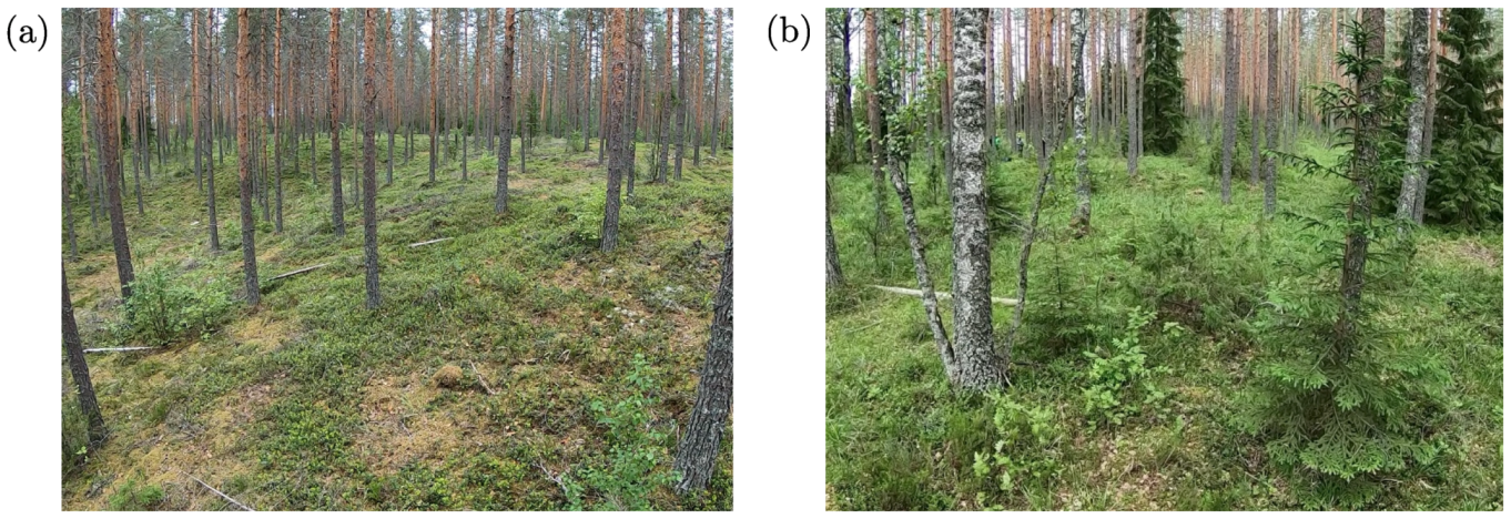
Note that all of the methods detected only a small fraction of the spruces (0.0–37.5%) present on the test sites, whereas the detection rate of pines was close to 100% for all of the measurements. Even though the detection rates for the ground-based mobile measurements and the above-canopy measurements were similar, the underlying factors determining the detection rates are quite different for these two classes of methods. For the ground-based/under-canopy MLS measurements, the most important factors limiting the detection of a particular tree are a small stem diameter and a poor stem visibility due to, e.g., branches. The pines on the test sites were dominant trees with visible and straight stems (see Figure 2a), and thus their detection rate was close to 100% based on the ground-based/under-canopy MLS measurements. On the other hand, basically all of the spruces on the test sites had an occluded stem and a small DBH (average 10 cm) as illustrated in Figure 2b. Therefore, it was difficult for the algorithms to detect the spruce stems and estimate their diameter using the stem detection-based approach employed in this study. However, if one is interested in detecting the spruces and not their stems, the completeness of spruce detection can be improved by using, e.g., methods based on vertical line fitting [14]. It is also noteworthy that it is most often the young spruces that tend to suffer from the stem occlusion problem. Typically, mature spruces relevant for the forest industry have visible stems at least close to the ground level, and thus stem-detection-based methods should work with a reasonable accuracy.

For the above-canopy UAV measurements, the high completeness of pine detection can be attributed to the fact that pines were mostly dominant trees whose tree tops were easily detectable from the canopy height model. On the other hand, the low completeness of spruce detection was due to the fact that most of the spruces on the test sites were shadowed by nearby located taller pines or birches. Thus, the canopy height model did not have a local maximum at the location of many of the spruces resulting in omission errors.

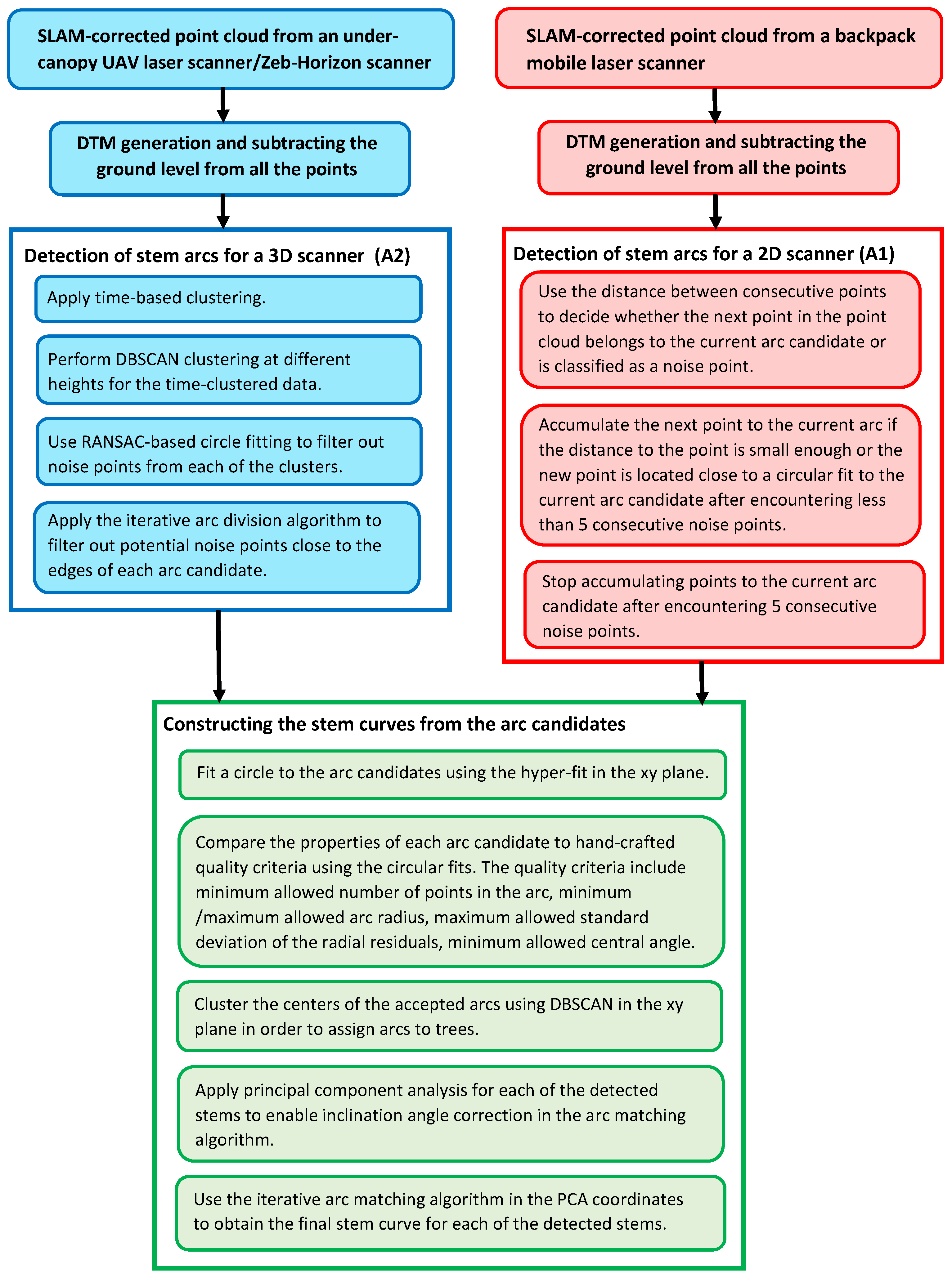
As an interesting note, the method based on backpack MLS resulted in the highest completeness rates, which was mainly due to the fact that the method was able to detect approximately one-third of the spruces, whereas the spruce detection rate was lower for the other methods. Importantly, the best results were obtained by using the arc detection algorithm that had been specifically designed for 2D laser scanners. As the arc finding algorithm for 2D scanners is based on scan line arc detection, it can apparently detect partly occluded stems with a better success rate as compared with the more general method designed for 3D scanners despite of the filtering steps in the more general algorithm.

4.2. Accuracy Comparison: DBH, Stem Curve, Tree Height, and Stem Volume

In this section, we present and discuss the results of stem diameter, tree height, and stem volume estimation for the different MLS measurements. The obtained values for bias and RMSE are summarized in

Table 7. The bias and root mean square error (RMSE) of DBH, tree height and stem volume estimation for the detected trees in the two plots based on the different mobile and airborne laser scanning methods. In the case of the under-canopy UAV LS, we have extracted the tree heights used for the stem volume computation from an above-canopy (AC) UAV measurement. In the table, we also compare field-measured DBHs and stem volumes against our reference measurements. The stem volumes of the field measurements were estimated by using the national Finnish allometric model [57] whose inputs are the field-measured DBH, tree height, and tree species. As field measured heights are used as the reference heights, the bias and RMSE of field measured heights is not presented in this table. Note that the units for the bias and RMSE are provided inside parentheses after each tree attribute in the leftmost column.

	Sparse Plot				Obstructed Plot
	Bias	Bias-%	RMSE	RMSE-%	Bias	Bias-%	RMSE	RMSE-%
Backpack BP-MLS-VUX1 A1
DBH (cm)	0.56	2.2	1.2	4.7	0.68	2.4	2.2	7.7
Height (m)	1.6	7.6	2.0	9.8	0.51	2.3	1.2	5.1
Volume (${\mathrm{dm}}^3$)	16	3.0	53	9.8	−2	−0.3	90	12.0
Backpack BP-MLS-VUX1 A2
DBH (cm)	0.69	2.7	1.2	4.7	0.92	3.1	1.9	6.5
Height (m)	1.4	6.7	1.5	7.1	0.55	2.3	1.0	4.2
Volume (${\mathrm{dm}}^3$)	67	12.1	83	15.1	73	9.0	93	11.5
Hand-held HH-MLS-ZEB
DBH (cm)	−0.39	−1.4	0.9	3.5	−0.44	−1.4	1.3	4.2
Height (m)	−0.16	−0.7	0.4	1.6	−1.1	−4.6	1.4	5.7
Volume (${\mathrm{dm}}^3$)	37	6.1	71	11.5	5	0.6	81	8.9
Under-canopy UC(&AC)-UAV-LS
DBH (cm)	0.34	1.3	0.6	2.3	0.12	0.4	1.1	3.5
Height (m)	0.34	1.5	0.5	2.4	−0.14	−0.5	0.8	3.2
Volume (${\mathrm{dm}}^3$)	24	3.9	65	10.6	36	4.1	97	11.0
Above-canopy UAV-LS-VQ480U
DBH (cm)	0.28	1.1	2.3	9.0	−0.95	−3.3	5.1	17.8
Height (m)	−0.03	−0.2	0.3	1.6	0.62	2.8	1.8	8.2
Volume (${\mathrm{dm}}^3$)	−6	−1.1	102	19.6	−83	−11.3	349	47.7
Above-canopy UAV-LS-RiCOP
DBH (cm)	−0.16	−0.6	2.3	9.0	−0.77	−2.8	5.1	18.1
Height (m)	0.03	0.1	0.5	2.3	0.82	3.7	1.6	7.2
Volume (${\mathrm{dm}}^3$)	−17	−3.4	97	18.7	−55	−7.7	360	50.2
Above-canopy UAV-LS-VUX1
DBH (cm)	−0.38	−1.5	2.2	8.8	−1.3	−4.5	5.6	19.7
Height (m)	0.0	0.0	0.4	2.0	0.71	3.2	1.5	6.6
Volume (${\mathrm{dm}}^3$)	−22	−4.3	103	19.9	−85	−11.6	392	53.6
Field measurements
DBH (cm)	0.00	0.02	1.0	4.2	−0.24	−0.96	0.79	3.1
Height (m)	-	-	-	-	-	-	-	-
Volume (${\mathrm{dm}}^3$)	−21	−4.3	59	12.4	−33	−5.2	144	23.1

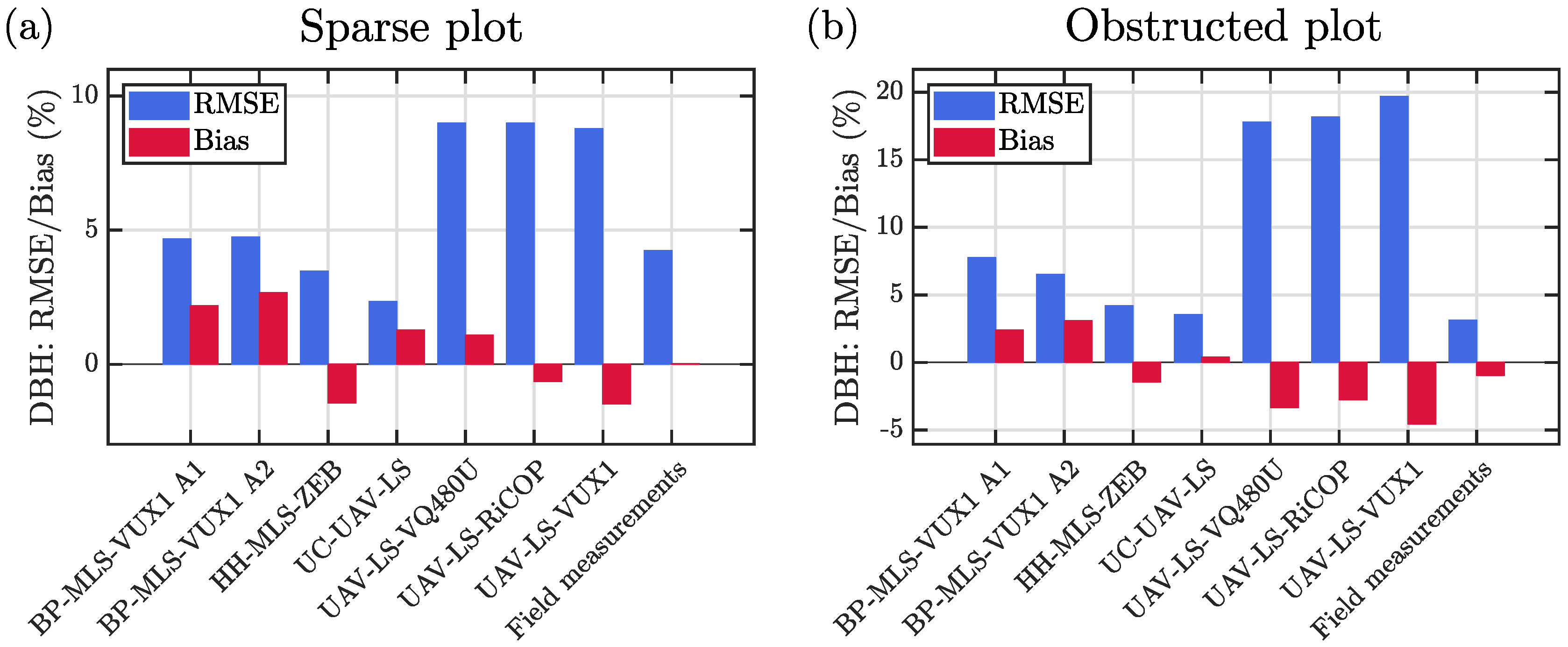
. In Figure 9, we show the relative bias and RMSE of the DBH estimates for the different methods in both the sparse and the obstructed plot. For each of the methods, the bias and RMSE were computed based on the trees that were detected with the particular method. In the sparse plot, the relative RMSE of DBH estimates varied between 2% and 5% for the ground-based/under-canopy MLS measurements, and the best results were obtained with the under-canopy UAV laser scanning system. In the obstructed plot, the relative RMSE of DBH estimation ranged between 4% and 8% for the ground-based/under-canopy MLS measurements, and again the best results were obtained with the under-canopy UAV system. Rather surprisingly, the RMSE of DBH estimation was higher for the backpack MLS system than for either the handheld laser scanner or the under-canopy UAV laser scanning system despite of the better ranging accuracy of the backpack laser scanner (see Figure 7). Importantly, the ground-based/under-canopy MLS measurements allowed us to estimate the DBH with an RMSE that was of similar magnitude as the error based on ordinary field measurements. For the ordinary field measurements, we obtained 4% for the relative RMSE of DBH estimation in the sparse plot, and 3% in the obstructed plot.

For the above-canopy UAV measurements, the RMSE of DBH estimation was significantly higher. In the sparse plot, all these three airborne laser scanning methods resulted in a relative RMSE of close to 10%, whereas the corresponding relative RMSE in the obstructed plot was close to 20%. The much higher error in the obstructed plot was due to the higher variation in the sizes of trees. Namely, the random forest model used in this study was observed to underestimate the diameters of large trees and overestimate the diameters of small trees. In general, the point density and season (leaf-off or leaf-on) had a small effect on the overall results.

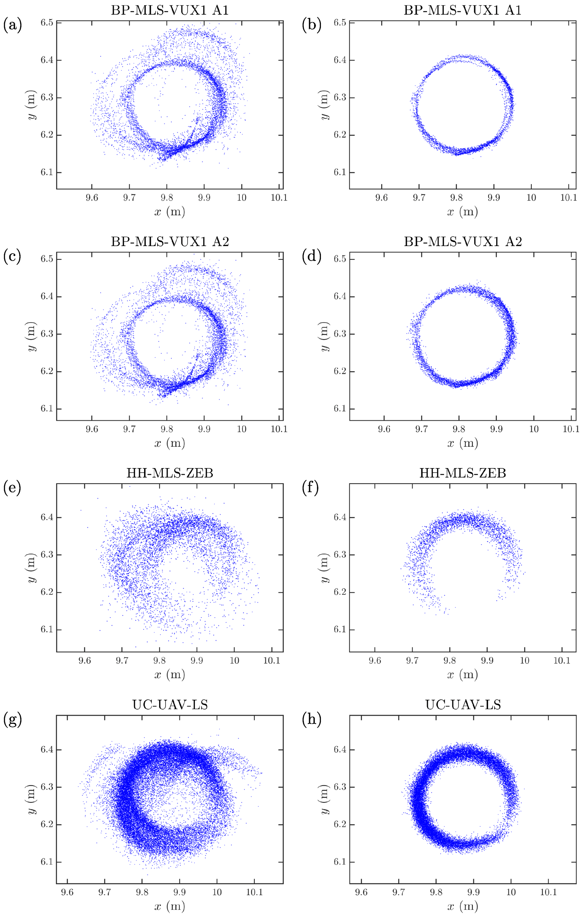
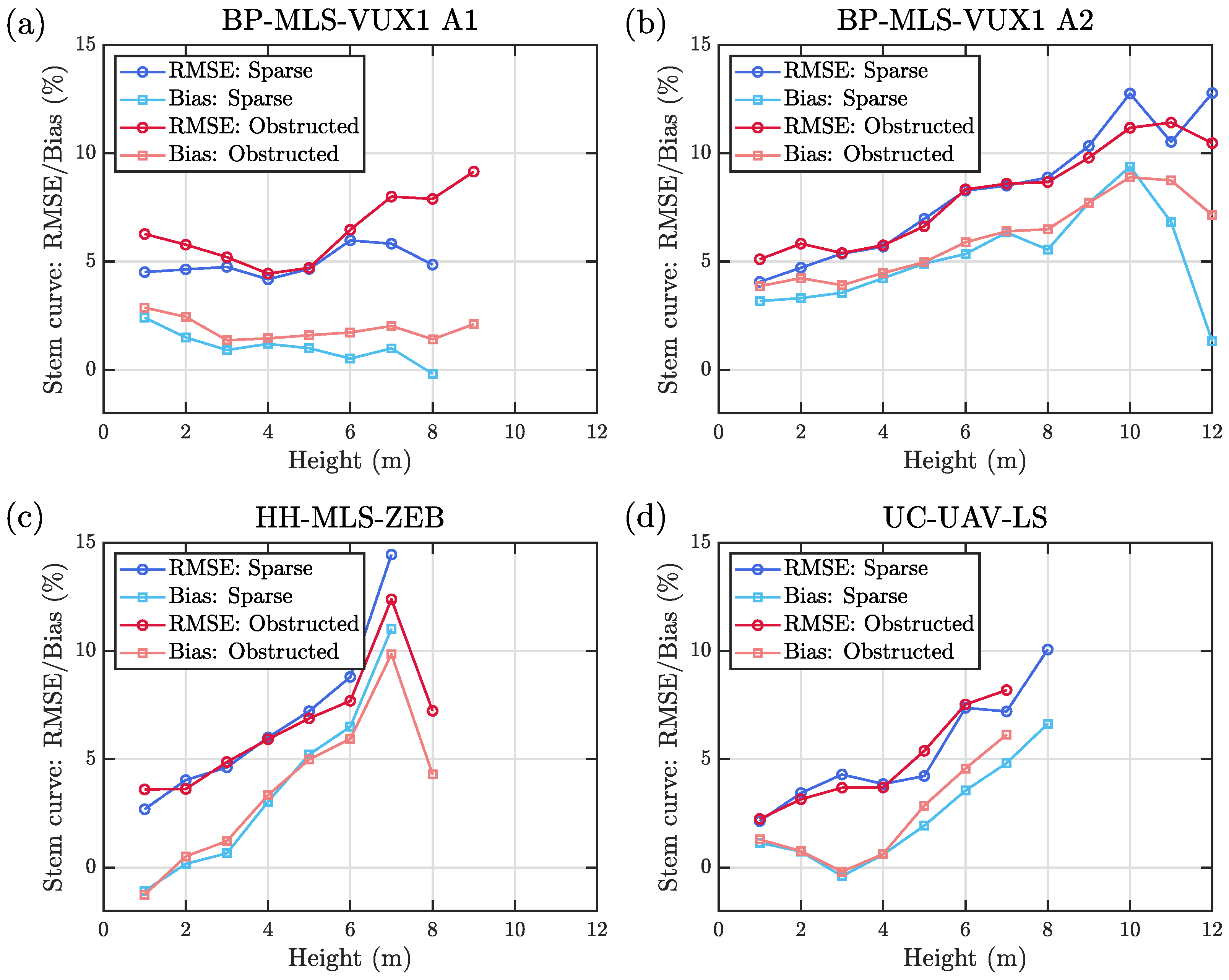
In Figure 10, we show the relative bias and RMSE for the stem curves estimated with the backpack MLS method, the handheld MLS method, and the under-canopy UAV method. When the backpack MLS data was processed using the stem arc detection algorithm for 2D scanners (A1), the bias of stem curve estimation was found to be close to zero and independent of measurement height. If we instead analyzed the same backpack MLS data using the stem arc detection algorithm for 3D scanners (A2), we observed that the bias of the estimated stem curves increased with increasing height. The same kind of behavior was also observed for the methods based on handheld MLS and under-canopy UAV LS, for which we also used the stem arc detection algorithm for 3D scanners. For the handheld MLS method, the bias and RMSE of the estimated stem curves increased the most rapidly as a function of height: even though the bias (RMSE) was essentially 0% (5%) at the breast height, the bias (RMSE) approached 10% (15%) already at the height of 7 m.

There are a few reasons that could potentially explain the height dependent bias and RMSE of the stem curve estimates. First, the average distance between the scanner and the reflected stem points increased as a function of the height of the stem arcs. This increased distance might have resulted in an increased transverse width of the laser pulse. Previously, it has been shown that the finite transverse width of the laser pulse can result in an overestimated diameter of the circular fit (see [49]). Interestingly, the bias of the stem curves extracted with the under-canopy UAV method attained its minimum value at the height of 3–4 m corresponding to a typical flying altitude of the UAV, whereas the smallest bias was recorded at the height of 1–2 m for the handheld Zeb-horizon system. This notion seems to support our hypothesis that the increased distance between the scanner and the stem arc is one major reason for the diameter overestimation at higher altitudes.

Second, the number of branches in a tree typically increased as a function of height, and thus noise points corresponding to the tree branches may have resulted in an overestimation of the stem diameter. We presume that the stem arc detection algorithm for 2D scanners was more robust against these effects since the point number threshold for an acceptable scan-line arc was set rather high. This helped to automatically filter out those stem arcs, for which the distance between the scanner and the arc was large. Additionally, we explicitly removed the two outermost points in each arc to mitigate edge effects as explained in Section 3.4.

Despite of the height dependent bias and RMSE, the accuracy of the MLS-based stem curve measurements is at the state-of-the-art level. We presume that the high accuracy of the stem curve measurements can be attributed to the arc-based approach utilized in the stem detection algorithm. When using this approach, the positional drift of the scanner hardly distorts individual arcs since the stem points in a single arc are obtained during a short period of time. Thus, the arc-based approach can be used to eliminate the positional drift of the scanner and to obtain high-quality stem diameter estimates by matching the individual stem arcs together.

We suspect that the arc matching process itself is actually not vital for obtaining accurate diameter estimates. One could probably obtain relatively good results by, e.g., computing the median of the arc diameters within each height interval for each stem model. However, the arc matching algorithm allows one to visualize the results of the stem curve extraction algorithm in an efficient fashion. This is of utmost importance in practical applications, where one must be able to assess the quality of the automatic measurements. Note also that the laser scanner must be clearly tilted with respect to the vertical plane, contrary to a TLS scanner, in order to ensure that the arc-based approach works efficiently.

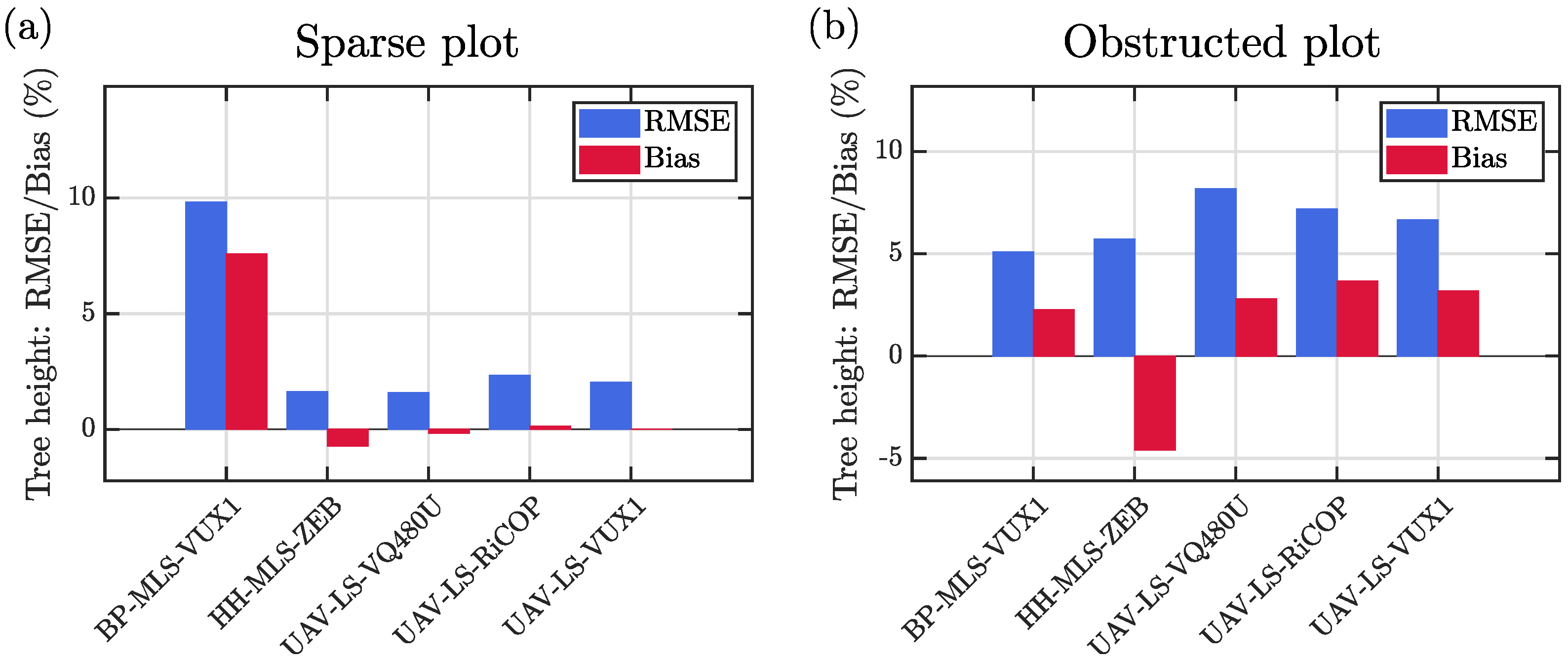
In Figure 11, we illustrate the bias and RMSE of the estimated tree heights for the backpack MLS method, the handheld MLS method and the three above-canopy UAV systems. In the sparse plot, the backpack laser scanner method overestimated tree heights by 1.6 m (7.6%), whereas the handheld laser scanner achieved a similar accuracy as the above-canopy UAV methods ($\mathrm{bias}-\%<1\%,\mathrm{RMSE}-\%\sim 2\%$). In the obstructed plot, the RMSE of height estimation was of similar magnitude for all the five methods ($\mathrm{RMSE}-\%\sim 5--8\%$), and actually the ground-based methods outperformed the methods based on above-canopy flying UAVs.

We presume that the severe overestimation of the tree heights by the backpack MLS method in the sparse plot was due to a failure of the graph-SLAM algorithm to perform matching in the vertical direction as discussed in [13]. This hypothesis is supported by the fact that the bias of the tree heights was observed to vary systematically with the tree location in the sparse plot. Additional support for this claim is provided by the fact that a similar overestimation of tree heights was not observed in the obstructed plot.

It is rather surprising that the accuracy of tree height estimation in the obstructed plot was slightly better for the ground-based mobile methods as compared with the methods based on above-canopy flying UAVs. The larger error in the above-canopy-based tree heights was mainly due to the fact that these methods severely overestimated the heights of those spruces that were detected from the canopy height model (see species-wise statistics in

Table 8. Species-specific bias and RMSE of DBH, tree height, and stem volume for the detected trees based on the different mobile and airborne laser scanning methods. In the case of the under-canopy UAV LS, we have extracted the tree heights used for the stem volume computation from an above-canopy (AC) UAV measurement. In the table, we also compare field-measured DBHs and stem volumes against our reference measurements. The stem volumes of the field measurements were estimated by using the national Finnish allometric model [57] whose inputs are the field-measured DBH, tree height, and tree species. It was not possible to estimate the bias and RMSE for field measured heights since they were used as the reference heights for all the measurements. Note that the units for the bias and RMSE are provided inside parentheses after each tree attribute in the leftmost column.

	Pines			Spruces			Birches
	Detected	Bias	RMSE	Detected	Bias	RMSE	Detected	Bias	RMSE
Backpack BP-MLS-VUX1 A1
DBH (cm)	69/69	0.5 (2.0%)	1.6 (5.9%)	4/11	1.8 (12.7%)	2.6 (19.0%)	5/5	0.7 (2.1%)	2.6 (8.3%)
Height (m)	69/69	1.0 (4.5%)	1.3 (5.7%)	4/11	2.6 (19.5%)	4.6 (34.3%)	5/5	0.6 (2.5%)	2.1 (9.4%)
Volume (${\mathrm{dm}}^3$)	69/69	10 (1.6%)	59 (9.2%)	4/11	30 (17.5%)	31 (18.0%)	5/5	−54 (−5.2%)	188 (17.9%)
Backpack BP-MLS-VUX1 A2
DBH (cm)	69/69	0.9 (3.3%)	1.5 (5.3%)	0/11	-	-	4/5	−0.8 −2.1%)	3.2 (8.9%)
Height (m)	69/69	1.1 (4.9%)	1.3 (6.0%)	0/11	-	-	4/5	−0.2 (−0.8%)	0.6 (2.4%)
Volume (${\mathrm{dm}}^3$)	69/69	72 (11.2%)	84 (13.2%)	0/11	-	-	4/5	41 (3.2%)	139 (10.7%)
Hand-held HH-MLS-ZEB
DBH (cm)	68/69	−0.4 (−1.3%)	1.1 (3.8%)	0/11	-	-	4/5	−1.3 (−3.4%)	1.5 (4.0%)
Height (m)	68/69	−0.6 (−2.5%)	1.0 (4.2%)	0/11	-	-	4/5	−1.2 (−4.8%)	1.3 (5.1%)
Volume (${\mathrm{dm}}^3$)	68/69	25 (3.6%)	73 (10.4%)	0/11	-	-	4/5	−25 (−1.8%)	106 (7.3%)
Under-canopy UC(&AC)-UAV-LS
DBH (cm)	69/69	0.3 (1.0%)	0.8 (2.7%)	1/11	0.5 (2.2%)	0.5 (2.2%)	4/5	−0.8 (−2.1%)	2.0 (5.2%)
Height (m)	69/69	0.1 (0.5%)	0.7 (2.8%)	1/11	1.6 (7.7%)	1.6 (7.7%)	4/5	−0.2 (−0.7%)	0.4 (1.7%)
Volume (${\mathrm{dm}}^3$)	69/69	24 (3.4%)	60 (8.5%)	1/11	88 (20.0%)	88 (20.0%)	4/5	117 (8.1%)	243 (16.8%)
UAV-LS-VQ480U
DBH (cm)	67/69	−0.4 (−1.3%)	2.9 (11.0%)	2/11	5.3 (33.0%)	7.1 (44.1%)	4/5	−2.5 (−7.2%)	10.5 (29.8%)
Height (m)	67/69	0.2 (1.0%)	0.7 (3.2%)	2/11	4.6 (31.7%)	6.7 (45.8%)	4/5	−0.6 (−2.5%)	1.0 (3.9%)
Volume (${\mathrm{dm}}^3$)	67/69	−35 (−5.9%)	140 (23.2%)	2/11	154 (78.9%)	221 (113.6%)	4/5	−282 (−23.3%)	917 (75.9%)
UAV-LS-RiCOP
DBH (cm)	68/69	−0.4 (−1.6%)	2.9 (11.0%)	3/11	3.0 (18.1%)	4.6 (27.6%)	4/5	−3.6 (−10.3%)	11.4 (32.3%)
Height (m)	68/69	0.3 (1.5%)	0.8 (3.6%)	3/11	3.6 (24.5%)	4.5 (30.8%)	4/5	−0.3 (−1.1%)	0.7 (2.9%)
Volume (${\mathrm{dm}}^3$)	68/69	−24 (−4.0%)	137 (22.7%)	3/11	92 (45.8%)	153 (76.3%)	4/5	−345 (−28.5%)	979 (81.0%)
UAV-LS-VUX1
DBH (cm)	69/69	−0.7 (−2.5%)	2.7 (10.2%)	2/11	3.9 (24.2%)	6.3 (39.4%)	4/5	−5.9 (−16.6%)	13.5 (38.4%)
Height (m)	69/69	0.3 (1.3%)	0.7 (3.2%)	2/11	4.1 (28.2%)	5.1 (35.1%)	4/5	−0.4 (−1.5%)	0.5 (2.1%)
Volume (${\mathrm{dm}}^3$)	69/69	−33 (−5.5%)	127 (21.2%)	2/11	103 (52.9%)	187 (95.8%)	4/5	−467 (−38.6%)	1093 (90.5%)
Field measurements
DBH (cm)	69/69	−0.2 (−0.9%)	0.8 (3.0%)	11/11	0.5 (4.9%)	1.5 (14.9%)	5/5	0.2 (0.6%)	0.8 (2.6%)
Height (m)	-	-	-	-	-	-	-	-	-
Volume (${\mathrm{dm}}^3$)	69/69	−23 (3.8%)	59 (9.8%)	11/11	−1 (−1.5%)	7 (9.2%)	5/5	−138 (−14.1%)	400 (41.0%)

). These spruces were, namely, located close to taller pines, which made it difficult to obtain accurate height estimates for them. This observation suggests that it is fairly difficult to estimate accurately the tree heights of suppressed trees using above-canopy collected point clouds. This problem could potentially be alleviated if the above-canopy point clouds were dense enough to enable locating the stems of trees. In this case, the stem locations could be used to guide the tree height estimation.

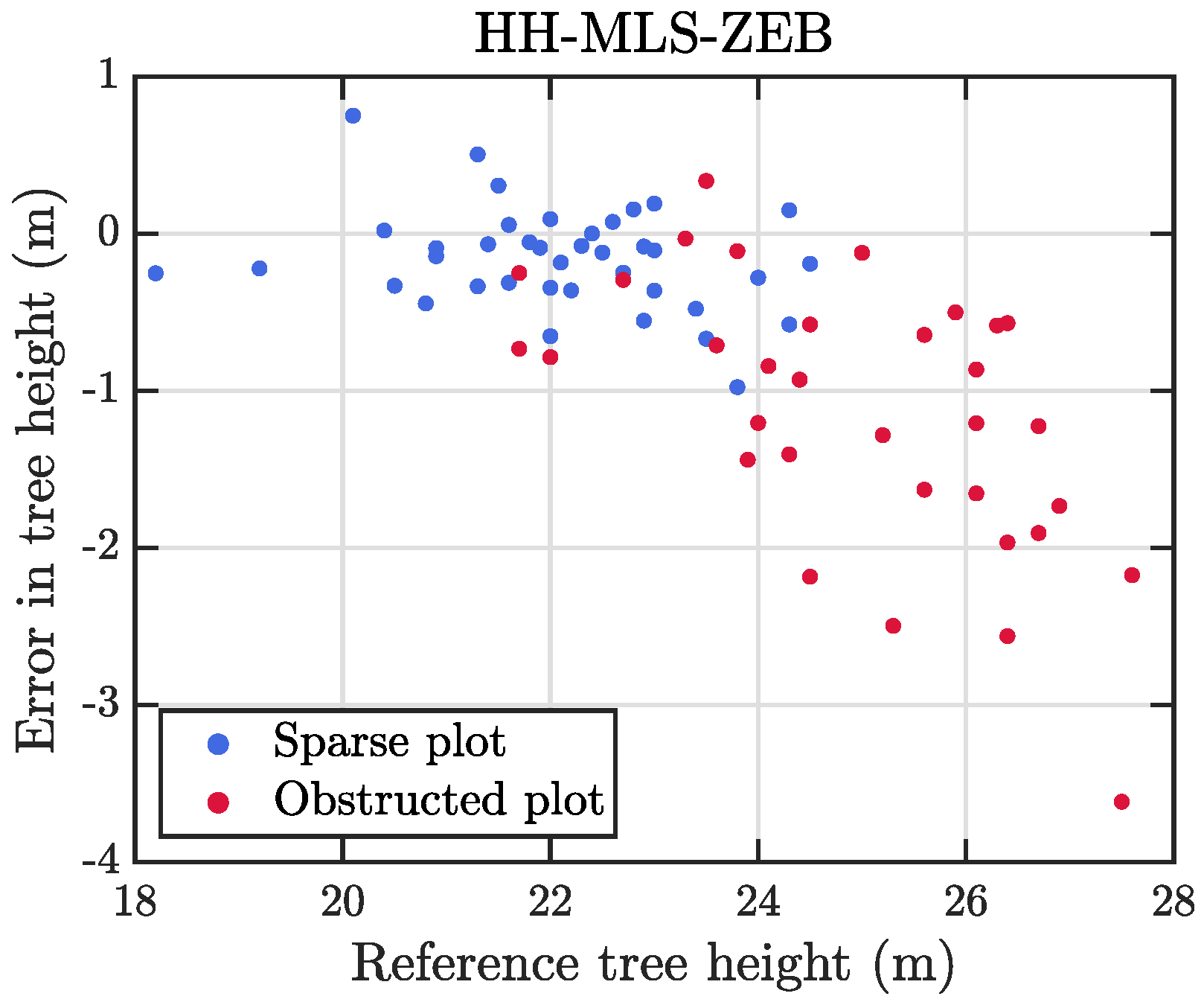
Additionally, we observed that the handheld Zeb-Horizon system systematically underestimated the heights of trees taller than 25 m as illustrated in Figure 12. Importantly, the systematic underestimation increased linearly with increasing height above the height of 25 m, which means that the range of the scanner is sufficient for measuring the tree heights up to the height of approximately 25 m in boreal forest conditions.

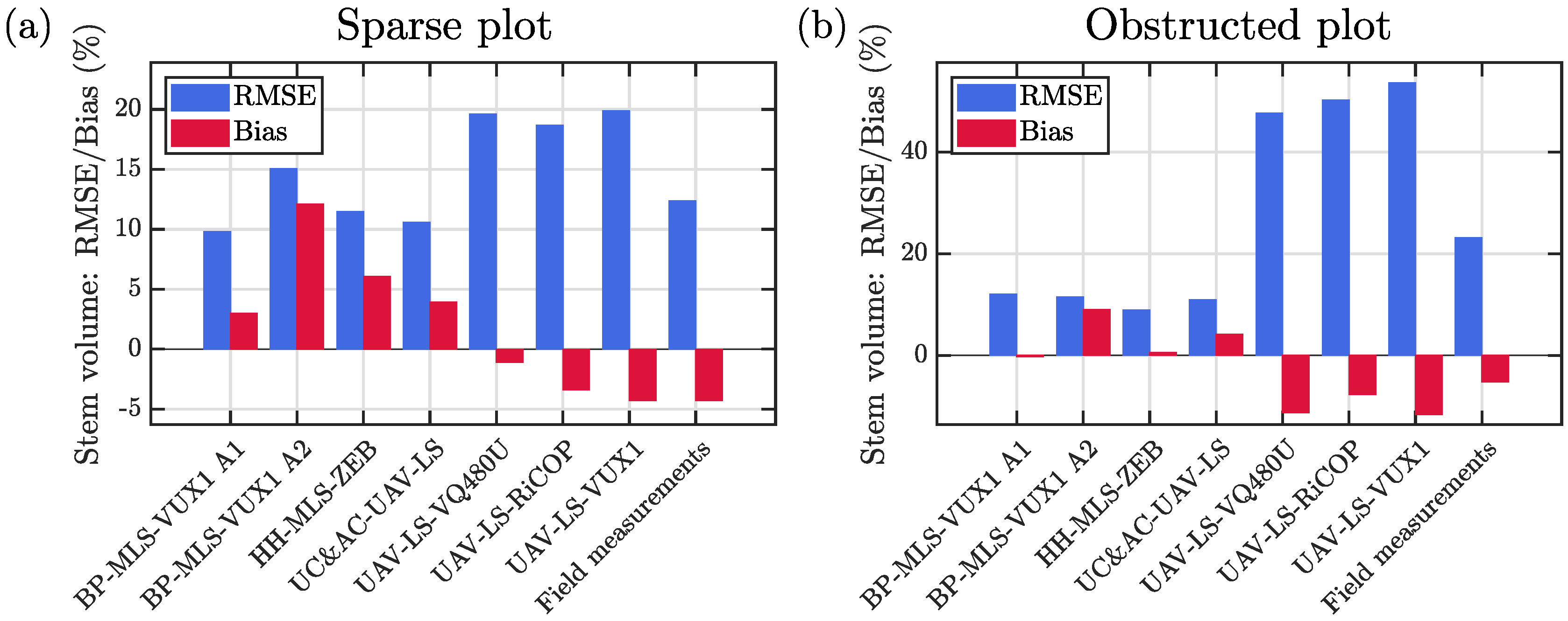
In Figure 13, we illustrate the bias and RMSE of stem volume estimates for the different methods. We can observe that the ground-based/under-canopy MLS methods slightly overestimated the stem volumes on average since these methods tended to overestimate the stem diameters as discussed above. For all of the ground-based/under-canopy MLS methods, the RMSE of the stem volume estimation was approximately 10–15% in both of the test sites. Note that the results for the handheld Zeb-Horizon scanner are perhaps deceptively good ($\mathrm{RMSE}-\%<10\%$) in the obstructed plot since the underestimation of tree heights was compensated by the overestimation of stem diameters. Note that the differences in the stem volume estimation accuracy were fairly small for the three ground-based/under-canopy MLS methods, and thus it is not possible to construct a conclusive ranking of these methods. One should also remember that the parameters of the algorithms were chosen heuristically meaning that it is possible that the parameters of the different methods might not be equally close to the optimal working point. Nevertheless, the errors in the stem volume estimates were of similar magnitude as results obtained with multi-scan TLS measurements in equivalent forest conditions [32].

Importantly, the errors in the stem volumes estimated with the ground-based/under-canopy MLS methods were at the same level or lower as the errors based on conventional stem volume measurements that had been conducted on the same test sites. In this study, the conventional volume measurements were carried out by inputting the field measured DBH, tree height and tree species into the Finnish national allometric model [57]. Importantly, the allometric model often tended to underestimate the volumes of large trees. For example, the volume of a large birch (DBH = 58 cm, V = 2.9 m³) in the obstructed plot was greatly underestimated by the allometric model (V = 2.0 m³). Note that this observation seems to suggest that it is beneficial to predict the stem volume using stem curve information from a wide height interval instead of using only the diameter at the breast height in the prediction of the stem volume. Naturally, this claim is true only if the stem curve can be extracted with a sufficient accuracy.

For the above-canopy laser scanning methods, the RMSE of stem volume estimation was approximately 20% in the sparse plot and close to 50% in the obstructed plot. The high error in the estimated stem volumes means that the above-canopy UAV LS methods cannot be used to derive the stem volume with a sufficient accuracy for individual tree level inventories unlike the ground-based/under-canopy MLS measurements. For these methods, the bias of the stem volume estimation was approximately $-10$% to 0%, which means that above-canopy UAV methods can, however, be used for collecting reference data for plot level forest inventories.

Additionally, it should be noted that the training data used for the above-canopy UAV methods was based on volumes computed with the Finnish national allometric model from field measured DBHs and tree heights on nearby plots. Therefore, the errors in the field estimated volumes propagated to the model. Nevertheless, the conclusions made in this section would not change had we used stem volumes extracted semi-manually from multi-scan TLS data to train the random forest models. Overall, we can conclude that the stem curve information is vital for estimating the stem volumes with a high accuracy at the individual tree level. Therefore, ground-based/under-canopy MLS methods have a clear advantage over methods based on above-canopy flying UAVs.

In Table 8, we further present the species-wise bias and RMSE of DBH, tree height, and stem volume estimation. As already discussed above, the results were the best for pines, as the pines were dominant trees with visible, straight, and circular stems. The worst results were obtained for spruces that were all relatively young and thus had an occluded stem with a DBH of approximately 10 cm. Since the spruces were located nearby taller pines and birches, the algorithms used for the tree height estimation often tended to overestimate their heights by several meters regardless of whether ground-based or above-canopy systems were used. Note that the relative bias and RMSE values for the spruce trees are inflated by the fact that the spruces were on average relatively small. For the birch trees, the ground-based/under-canopy MLS methods managed to extract the stem volume with a good accuracy (RMSE = 7–17%), whereas the above-canopy LS measurements failed to provide accurate information of their DBH or stem volume. However, it is noteworthy that the results for the birch trees depended largely on how accurately the methods managed to model the very large birch located in the obstructed test site.

Overall, the number of spruces and birches on the test sites was relatively low, and therefore, one should not draw too far-reaching conclusions based on the data provided in Table 8. Importantly, the spruces on the test sites did not include any mature trees with a partly visible stem. Therefore, the results presented in Table 8 probably give a too pessimistic view of the performance of the methods when it comes to detecting and modeling mature spruces that are relevant for the forest industry.

In

Table 9. Statistics of omitted trees for the different mobile and airborne laser scanning methods. The statistics include the omitted reference trees from both of the test sites. The last column of the table represents the total stem volume of the omitted trees as compared with the total reference stem volume on both of the test sites combined.

System	Number of Omitted Trees				DBH (cm)		Height (m)		Of Total Volume (%)
	All	Pines	Spruces	Birches	Mean	Std. Dev.	Mean	Std. Dev.
BP-MLS-VUX1 A1	7	0	7	0	9.6	3.6	8.6	2.5	0.6
BP-MLS-VUX1 A2	12	0	11	1	11.1	5.1	10.5	4.3	2.1
HH-MLS-ZEB	13	1	11	1	14.0	6.5	12.8	5.0	3.6
UC-UAV-LS	11	0	10	1	12.0	4.7	11.2	3.4	1.8
UAV-LS-VQ480U	12	2	9	1	11.0	6.6	10.2	5.0	2.6
UAV-LS-RiCOP	10	1	8	1	9.0	4.8	9.0	4.5	1.2
UAV-LS-VUX1	10	0	9	1	8.7	4.2	8.5	3.4	0.9

, we present statistics of the trees that were not detected by the different MLS methods. Importantly, the omitted trees were relatively small with a mean DBH in the range of 8 to 14 cm depending on the method. Importantly, the total volume of the omitted trees varied between 0.6% and 3.6% of the total stem volume present on the test sites. The best result (0.6%) was obtained for the backpack laser scanning system, whereas the worst result (3.6%) was obtained for the handheld scanner. Nevertheless, the total volume of the omitted trees was small for all the different methods meaning that all of them were able to detect the trees that were relevant from the point of view of forest industry.

5. Conclusions

In this study, we investigated the accuracy of two ground-based mobile laser scanning methods, a method based on under-canopy UAV laser scanning and three above-canopy UAV laser scanning methods for field reference data collection at the individual tree level. Herein, we found three approaches based on a backpack, handheld, and an under-canopy UAV laser scanner system that enabled the estimation of DBH, stem curve and stem volume with a sufficient accuracy for operational applications in easy and medium-difficult boreal forest conditions. We found that the RMSE of DBH estimation varied between 2% and 8% for the different ground-based/under-canopy MLS measurements depending on the difficulty of the forest conditions. Additionally, the RMSE of stem volume estimation was found to vary between 9–15%. As the bias of DBH and stem volume estimation was small for all of these three techniques, these methods could also be used to provide plot level estimates. Importantly, these three MLS methods enabled stem volume estimation with an accuracy that was similar or even slightly better than the corresponding results obtained with ordinary field measurements and the Finnish national allometric model. Additionally, the obtained errors of stem volume estimation were on par with results obtained with multi-scan TLS measurements in similar forest conditions.

Using the data collected with the three above-canopy UAV laser scanning systems and a random forest model trained on reference data from nearby plots, we were able to estimate the DBH of individual trees with a RMSE of 10–20% and the stem volume with a RMSE ranging from 20% to 50% depending on the difficulty of the forest conditions. Thus, the accuracy of above-canopy UAV laser scanning measurements was found to be insufficient for field reference data collection at the individual tree level. Importantly, point cloud data collected with the under-canopy flying UAV combined with tree height information could be used to derive stem volume estimates with a significantly better accuracy as compared with the methods based on above-canopy flying UAVs.

Furthermore, we observed that the backpack laser scanning system and the handheld Zeb-Horizon scanner could be used for sufficiently accurate tree height measurements (RMSE = 2–10%). We found that the accuracy of the MLS-based tree heights was similar as compared with the tree heights estimated from above-canopy laser scanning measurements in medium–difficult boreal forest conditions. In such forests, the information of stem location provided additional value for the tree height estimation since a large proportion of the smaller spruce trees was shadowed by dominant pines. However, the handheld Zeb-Horizon scanner underestimated the heights of trees above 25 m, and should not be used to measure the heights of trees much taller than 25 m.

For all of the six methods, the detection rate for spruces was much lower (0–40%) as compared with pines (~100%) and birches (80–100%), which can be attributed to the relatively small size of the spruces and, therefore, the severe occlusion of their stems. Future studies should focus on spruces of all sizes and dense, complex canopies in order to be able to reach practical performance for field inventories. Developments in SLAM algorithms and autonomous UAV are also needed to further improve the accuracy and practicality of the presented methods. In conclusion, the findings are important steps towards future individual-tree-based laser scanning forest inventories.

References

1. Hyyppä, J.; Hyyppä, H.; Inkinen, M.; Engdahl, M.; Linko, S.; Zhu, Y.H. Accuracy comparison of various remote sensing data sources in the retrieval of forest stand attributes. Forest Ecol. Manag. 2000, 128, 109–120. [Google Scholar] [CrossRef]
2. Yu, X.; Hyyppä, J.; Karjalainen, M.; Nurminen, K.; Karila, K.; Vastaranta, M.; Kankare, V.; Kaartinen, H.; Holopainen, M.; Honkavaara, E.; et al. Comparison of laser and stereo optical, SAR and InSAR point clouds from air-and space-borne sources in the retrieval of forest inventory attributes. Remote Sens. 2015, 7, 15933–15954. [Google Scholar] [CrossRef] [Green Version]
3. Clark, N.A.; Wynne, R.H.; Schmoldt, D.L.; Winn, M. An assessment of the utility of a non-metric digital camera for measuring standing trees. Comput. Electron. Agric. 2000, 28, 151–169. [Google Scholar]
4. Gougeon, F.A.; Leckie, D.G. Individual tree crown image analysis—a step towards precision forestry. In Proceedings of the First International Precision Forestry Cooperative Symposium, Seattle, WA, USA, 17–20 June 2001; pp. 43–49. [Google Scholar]
5. Luoma, V.; Saarinen, N.; Wulder, M.A.; White, J.C.; Vastaranta, M.; Holopainen, M.; Hyyppä, J. Assessing precision in conventional field measurements of individual tree attributes. Forests 2017, 8, 38. [Google Scholar] [CrossRef] [Green Version]
6. Larjavaara, M.; Muller-Landau, H.C. Measuring tree height: A quantitative comparison of two common field methods in a moist tropical forest. Method. Ecol. Evol. 2013, 4, 793–801. [Google Scholar] [CrossRef]
7. Bauwens, S.; Bartholomeus, H.; Calders, K.; Lejeune, P. Forest inventory with terrestrial LiDAR: A comparison of static and hand-held mobile laser scanning. Forests 2016, 7, 127. [Google Scholar]
8. Bienert, A.; Georgi, L.; Kunz, M.; Maas, H.G.; von Oheimb, G. Comparison and combination of mobile and terrestrial laser scanning for natural forest inventories. Forests 2018, 9, 395. [Google Scholar] [CrossRef] [Green Version]
9. Brede, B.; Lau, A.; Bartholomeus, H.; Kooistra, L. Comparing RIEGL RiCOPTER UAV LiDAR derived canopy height and DBH with terrestrial LiDAR. Sensors 2017, 17, 2371. [Google Scholar] [CrossRef]
10. Cabo, C.; Del Pozo, S.; Rodríguez-Gonzálvez, P.; Ordóñez, C.; González-Aguilera, D. Comparing terrestrial laser scanning (TLS) and wearable laser scanning (WLS) for individual tree modeling at plot level. Remote Sens. 2018, 10, 540. [Google Scholar] [CrossRef] [Green Version]
11. Liang, X.; Wang, Y.; Pyörälä, J.; Lehtomäki, M.; Yu, X.; Kaartinen, H.; Kukko, A.; Honkavaara, E.; Issaoui, A.E.; Nevalainen, O.; et al. Forest in situ observations using unmanned aerial vehicle as an alternative of terrestrial measurements. Forest Ecosyst. 2019, 6, 20. [Google Scholar]
12. Hunčaga, M.; Chudá, J.; Tomaštík, J.; Slámová, M.; Koreň, M.; Chudỳ, F. The Comparison of Stem Curve Accuracy Determined from Point Clouds Acquired by Different Terrestrial Remote Sensing Methods. Remote Sens. 2020, 12, 2739. [Google Scholar] [CrossRef]
13. Hyyppä, E.; Kukko, A.; Kaijaluoto, R.; White, J.C.; Wulder, M.A.; Pyörälä, J.; Liang, X.; Yu, X.; Wang, Y.; Kaartinen, H.; et al. Accurate derivation of stem curve and volume using backpack mobile laser scanning. ISPRS J. Photogr. Remote Sens. 2020, 161, 246–262. [Google Scholar] [CrossRef]
14. Hyyppä, E.; Hyyppä, J.; Hakala, T.; Kukko, A.; Wulder, M.A.; White, J.C.; Pyörälä, J.; Yu, X.; Wang, Y.; Virtanen, J.P.; et al. Under-canopy UAV laser scanning for accurate forest field measurements. ISPRS J. Photogr. Remote Sens. 2020, 164, 41–60. [Google Scholar]
15. Balenović, I.; Liang, X.; Jurjević, L.; Hyyppä, J.; Seletković, A.; Kukko, A. Hand-Held Personal Laser Scanning–Current Status and Perspectives for Forest Inventory Application. Croat. J. Forest Eng. 2020, TBA. [Google Scholar]
16. Liang, X.; Hyyppä, J.; Kaartinen, H.; Lehtomäki, M.; Pyörälä, J.; Pfeifer, N.; Holopainen, M.; Brolly, G.; Francesco, P.; Hackenberg, J.; et al. International benchmarking of terrestrial laser scanning approaches for forest inventories. ISPRS J. Photogr. Remote Sens. 2018, 144, 137–179. [Google Scholar] [CrossRef]
17. Dai, W.; Yang, B.; Liang, X.; Dong, Z.; Huang, R.; Wang, Y.; Li, W. Automated fusion of forest airborne and terrestrial point clouds through canopy density analysis. ISPRS J. Photogr. Remote Sens. 2019, 156, 94–107. [Google Scholar] [CrossRef]
18. Srinivasan, S.; Popescu, S.C.; Eriksson, M.; Sheridan, R.D.; Ku, N.W. Multi-temporal terrestrial laser scanning for modeling tree biomass change. Forest Ecol. Manag. 2014, 318, 304–317. [Google Scholar] [CrossRef]
19. Vastaranta, M.; Saarinen, N.; Yrttimaa, T.; Kankare, V.; Junttila, S. Monitoring forests in space and time using close-range sensing. Preprints 2020. [Google Scholar] [CrossRef]
20. Hackenberg, J.; Wassenberg, M.; Spiecker, H.; Sun, D. Non destructive method for biomass prediction combining TLS derived tree volume and wood density. Forests 2015, 6, 1274–1300. [Google Scholar] [CrossRef]
21. Saarinen, N.; Kankare, V.; Vastaranta, M.; Luoma, V.; Pyörälä, J.; Tanhuanpää, T.; Liang, X.; Kaartinen, H.; Kukko, A.; Jaakkola, A.; et al. Feasibility of Terrestrial laser scanning for collecting stem volume information from single trees. ISPRS J. Photogr. Remote Sens. 2017, 123, 140–158. [Google Scholar]
22. Tomaštík, J.; Saloň, Š.; Tunák, D.; Chudỳ, F.; Kardoš, M. Tango in forests–An initial experience of the use of the new Google technology in connection with forest inventory tasks. Comput. Electron. Agric. 2017, 141, 109–117. [Google Scholar] [CrossRef]
23. Hyyppä, J.; Virtanen, J.P.; Jaakkola, A.; Yu, X.; Hyyppä, H.; Liang, X. Feasibility of Google Tango and Kinect for crowdsourcing forestry information. Forests 2018, 9, 6. [Google Scholar] [CrossRef] [Green Version]
24. Fan, Y.; Feng, Z.; Mannan, A.; Khan, T.U.; Shen, C.; Saeed, S. Estimating tree position, diameter at breast height, and tree height in real-time using a mobile phone with RGB-D SLAM. Remote Sens. 2018, 10, 1845. [Google Scholar] [CrossRef] [Green Version]
25. Kaartinen, H.; Hyyppä, J.; Vastaranta, M.; Kukko, A.; Jaakkola, A.; Yu, X.; Pyörälä, J.; Liang, X.; Liu, J.; Wang, Y.; et al. Accuracy of kinematic positioning using global satellite navigation systems under forest canopies. Forests 2015, 6, 3218–3236. [Google Scholar] [CrossRef]
26. Durrant-Whyte, H.; Bailey, T. Simultaneous localization and mapping: Part I. IEEE Robot. Autom. Mag. 2006, 13, 99–110. [Google Scholar] [CrossRef] [Green Version]
27. Forsman, M.; Holmgren, J.; Olofsson, K. Tree stem diameter estimation from mobile laser scanning using line-wise intensity-based clustering. Forests 2016, 7, 206. [Google Scholar]
28. Kukko, A.; Kaijaluoto, R.; Kaartinen, H.; Lehtola, V.V.; Jaakkola, A.; Hyyppä, J. Graph SLAM correction for single scanner MLS forest data under boreal forest canopy. ISPRS J. Photogr. Remote Sens. 2017, 132, 199–209. [Google Scholar] [CrossRef]
29. Pierzchała, M.; Giguère, P.; Astrup, R. Mapping forests using an unmanned ground vehicle with 3D LiDAR and graph-SLAM. Computers Electron. Agric. 2018, 145, 217–225. [Google Scholar] [CrossRef]
30. Fan, Y.; Feng, Z.; Shen, C.; Khan, T.U.; Mannan, A.; Gao, X.; Chen, P.; Saeed, S. A trunk-based SLAM backend for smartphones with online SLAM in large-scale forest inventories. ISPRS J. Photogr. Remote Sens. 2020, 162, 41–49. [Google Scholar]
31. Del Perugia, B.; Giannetti, F.; Chirici, G.; Travaglini, D. Influence of Scan Density on the Estimation of Single-Tree Attributes by Hand-Held Mobile Laser Scanning. Forests 2019, 10, 277. [Google Scholar]
32. Liang, X.; Kukko, A.; Hyyppä, J.; Lehtomäki, M.; Pyörälä, J.; Yu, X.; Kaartinen, H.; Jaakkola, A.; Wang, Y. In-situ measurements from mobile platforms: An emerging approach to address the old challenges associated with forest inventories. ISPRS J. Photogr. Remote Sens. 2018, 143, 97–107. [Google Scholar] [CrossRef]
33. Čerňava, J.; Mokroš, M.; Tuček, J.; Antal, M.; Slatkovská, Z. Processing Chain for Estimation of Tree Diameter from GNSS-IMU-Based Mobile Laser Scanning Data. Remote Sens. 2019, 11, 615. [Google Scholar]
34. Zhao, Y.; Hu, Q.; Li, H.; Wang, S.; Ai, M. Evaluating Carbon Sequestration and PM2. 5 Removal of Urban Street Trees Using Mobile Laser Scanning Data. Remote Sens. 2018, 10, 1759. [Google Scholar] [CrossRef] [Green Version]
35. Cui, J.Q.; Lai, S.; Dong, X.; Chen, B.M. Autonomous navigation of UAV in foliage environment. J. Intell. Robot. Syst. 2016, 84, 259–276. [Google Scholar]
36. Vandapel, N.; Kuffner, J.; Amidi, O. Planning 3-d path networks in unstructured environments. In Proceedings of the 2005 IEEE International Conference on Robotics and Automation, Barcelona, Spain, 18–22 April 2005; pp. 4624–4629. [Google Scholar]
37. Vian, J.L.; Przybylko, J. Tree Metrology System. U.S. Patent 9,198,363, 12 December 2012. [Google Scholar]
38. Chisholm, R.A.; Cui, J.; Lum, S.K.; Chen, B.M. UAV LiDAR for below-canopy forest surveys. J. Unmanned Veh. Syst. 2013, 1, 61–68. [Google Scholar] [CrossRef] [Green Version]
39. Kuželka, K.; Surovỳ, P. Mapping Forest Structure Using UAS inside Flight Capabilities. Sensors 2018, 18, 2245. [Google Scholar] [CrossRef] [Green Version]
40. Krisanski, S.; Taskhiri, M.S.; Turner, P. Enhancing Methods for Under-Canopy Unmanned Aircraft System based Photogrammetry in Complex Forests for Tree Diameter Measurement. Remote Sens. 2020, 12, 1652. [Google Scholar] [CrossRef]
41. Jaakkola, A.; Hyyppä, J.; Yu, X.; Kukko, A.; Kaartinen, H.; Liang, X.; Hyyppä, H.; Wang, Y. Autonomous collection of forest field reference—The outlook and a first step with UAV laser scanning. Remote Sens. 2017, 9, 785. [Google Scholar] [CrossRef] [Green Version]
42. Wieser, M.; Mandlburger, G.; Hollaus, M.; Otepka, J.; Glira, P.; Pfeifer, N. A case study of UAS borne laser scanning for measurement of tree stem diameter. Remote Sens. 2017, 9, 1154. [Google Scholar] [CrossRef] [Green Version]
43. Harikumar, A.; Bovolo, F.; Bruzzone, L. An approach to conifer stem localization and modeling in high density airborne LiDAR data. In Image and Signal Processing for Remote Sensing XXIII; International Society for Optics and Photonics: Bellingham, WA, USA, 2017; Volume 10427, p. 104270Q. [Google Scholar]
44. Puliti, S.; Breidenbach, J.; Astrup, R. Estimation of Forest Growing Stock Volume with UAV Laser Scanning Data: Can It Be Done without Field Data? Remote Sens. 2020, 12, 1245. [Google Scholar] [CrossRef] [Green Version]
45. Jaakkola, A.; Hyyppä, J.; Kukko, A.; Yu, X.; Kaartinen, H.; Lehtomäki, M.; Lin, Y. A low-cost multi-sensoral mobile mapping system and its feasibility for tree measurements. ISPRS J. Photogr. Remote Sens. 2010, 65, 514–522. [Google Scholar] [CrossRef]
46. Wallace, L.; Lucieer, A.; Watson, C.; Turner, D. Development of a UAV-LiDAR system with application to forest inventory. Remote Sens. 2012, 4, 1519–1543. [Google Scholar] [CrossRef] [Green Version]
47. Wallace, L.; Musk, R.; Lucieer, A. An assessment of the repeatability of automatic forest inventory metrics derived from UAV-borne laser scanning data. IEEE Trans. Geosci. Remote Sens. 2014, 52, 7160–7169. [Google Scholar] [CrossRef]
48. Holmgren, J.; Tulldahl, M.; Nordlöf, J.; Willén, E.; Olsson, H. Mobile Laser Scanning for Estimating Tree Stem Diameter Using Segmentation and Tree Spine Calibration. Remote Sens. 2019, 11, 2781. [Google Scholar] [CrossRef] [Green Version]
49. Forsman, M.; Börlin, N.; Olofsson, K.; Reese, H.; Holmgren, J. Bias of cylinder diameter estimation from ground-based laser scanners with different beam widths: A simulation study. ISPRS J. Photogr. Remote Sens. 2018, 135, 84–92. [Google Scholar]
50. Ester, M.; Kriegel, H.P.; Sander, J.; Xu, X. A Density-Based Algorithm for Discovering Clusters in Large Spatial Databases With Noise. 1996, Volume 96, pp. 226–231. Available online: https://www.aaai.org/Papers/KDD/1996/KDD96-037.pdf?source=post_page (accessed on 10 October 2020).
51. Fischler, M.A.; Bolles, R.C. Random sample consensus: A paradigm for model fitting with applications to image analysis and automated cartography. Commun. ACM 1981, 24, 381–395. [Google Scholar] [CrossRef]
52. Al-Sharadqah, A.; Chernov, N. Error analysis for circle fitting algorithms. Electronic J. Stat. 2009, 3, 886–911. [Google Scholar] [CrossRef]
53. Breiman, L. Random forests. Machine Learn. 2001, 45, 5–32. [Google Scholar] [CrossRef] [Green Version]
54. Yu, X.; Hyyppä, J.; Vastaranta, M.; Holopainen, M.; Viitala, R. Predicting individual tree attributes from airborne laser point clouds based on the random forests technique. ISPRS J. Photogr. Remote Sens. 2011, 66, 28–37. [Google Scholar] [CrossRef]
55. Vauhkonen, J.; Korpela, I.; Maltamo, M.; Tokola, T. Imputation of single-tree attributes using airborne laser scanning-based height, intensity, and alpha shape metrics. Remote Sens. Environ. 2010, 114, 1263–1276. [Google Scholar] [CrossRef]
56. Yu, X.; Hyyppä, J.; Kukko, A.; Maltamo, M.; Kaartinen, H. Change detection techniques for canopy height growth measurements using airborne laser scanner data. Photogr. Eng. Remote Sens. 2006, 72, 1339–1348. [Google Scholar] [CrossRef]
57. Laasasenaho, J. Taper Curve and Volume Functions for Pine, Spruce and Birch; Metsäntutkimuslaitos: Helsinki, Finland, 1982. [Google Scholar]
Figure 1. Photographs of (a) the sparse plot and (b) the obstructed plot.
Remotesensing 12 03327 g001
Figure 2. Example trees for each of the three tree species present in the two plots. (a) Pine. (b) Spruce. (c) Two birches. Note that the small birch on the right side of the large birch has a DBH below 5 cm and was thus not included in the set of reference trees.
Remotesensing 12 03327 g002
Figure 3. Photographs of (a) the backpack mobile laser scanning unit (BP-MLS-VUX1), (b) the handheld ZEB-Horizon laser scanner (HH-MLS-ZEB), (c) the under-canopy UAV laser scanning system (UC-UAV-LS), and (d) the RiCopter laser scanning system (UAV-LS-RiCOP).
Remotesensing 12 03327 g003
Figure 4. (a,b) Trajectory (white line) of the scanner for the measurements conducted with the backpack BP-MLS-VUX1 system (a) in the sparse plot and (b) in the obstructed plot. (c,d) Trajectory (white line) of the scanner for the measurements conducted with the handheld HH-MLS-ZEB system (c) in the sparse plot and (d) in the obstructed plot. (e,f) Trajectory (white line) of the scanner for the measurements conducted with the under-canopy UC-UAV-LS system (e) in the sparse plot and (f) in the obstructed plot. In all the panels, the red circles denote the positions of reference trees.
Remotesensing 12 03327 g004
Figure 5. (a,c,e) Simultaneous localization and mapping (SLAM)-corrected point clouds from a 20 m × 20 m region within the sparse plot collected with (a) the backpack BP-MLS-VUX1 system, (c) the handheld HH-MLS-ZEB system, and (e) the under-canopy UC-UAV-LS system. (b,d,f) Cross sections of the SLAM-corrected point clouds in the height interval z [ 2 m , 3 m ] showcasing the stems of three pine trees in the point cloud collected with (b) the BP-MLS-VUX1 system, (d) the HH-MLS-ZEB system, and (f) the UC-UAV-LS system.
Remotesensing 12 03327 g005
Figure 6. Flow chart of the stem curve extraction algorithm used for the backpack laser scanner, under-canopy UAV laser scanner, and handheld laser scanner. The algorithms are based on our previous work [13,14].
Remotesensing 12 03327 g006
Figure 7. (a,c,e,g) Cross section of the SLAM-corrected point cloud modeling a pine tree in the height range z [ 2.0 m , 2.5 m ] m collected with (a,c) the backpack BP-MLS-VUX1 system, (e) the handheld HH-MLS-ZEB system, and (g) the under-canopy UC-UAV-LS system. Note that the panels (a,c) are essentially the same figure. (b,d,f,h) The corresponding pine stem models after applying the arc extraction algorithm and the iterative arc matching algorithm (b) for the data collected with the backpack BP-MLS-VUX1 system and processed using the 2D arc extraction algorithm (A1), (d) for the data collected with the backpack BP-MLS-VUX1 system and processed using the 3D arc extraction algorithm (A2), (f) for the data collected with the handheld HH-MLS-ZEB system and processed using the 3D arc extraction algorithm, and (h) for the data collected with the under-canopy UC-UAV-LS system and processed using the 3D arc extraction algorithm.
Remotesensing 12 03327 g007
Figure 8. Point clouds of the sparse test site obtained with the different above-canopy flying UAV systems: (a) UAV-LS-VQ480U, (b) UAV-LS-RiCOP, and (c) UAV-LS-VUX1.
Remotesensing 12 03327 g008
Figure 9. Relative bias and RMSE of DBH estimation at the individual tree level for the different MLS methods (a) in the sparse plot and (b) in the obstructed plot. BP, HH, and UC stand for backpack, handheld, and under-canopy, respectively. Note that the scales of the y axes are different in panels (a,b).
Remotesensing 12 03327 g009
Figure 10. Relative bias and RMSE of the stem curve estimates as a function of height from the ground level for (a) the data collected with the backpack BP-MLS-VUX1 system and processed using the 2D arc extraction algorithm, (b) the data collected with the backpack BP-MLS-VUX1 system and processed using the 3D arc extraction algorithm (A2), (c) the data collected with the handheld HH-MLS-ZEB system and processed using the 3D arc extraction algorithm, and (d) for the data collected with the under-canopy UC-UAV-LS system and processed using the 3D arc extraction algorithm. Note that the bias and RMSE of the stem curve estimates are shown for all the height intervals, for which the stem curve could be estimated for at least 5 trees within each plot.
Remotesensing 12 03327 g010
Figure 11. Relative bias and RMSE of tree height estimation at the individual tree level for the different methods (a) in the sparse plot and (b) in the obstructed plot. BP and HH stand for backpack and handheld, respectively. Note that the scales of the y axes are different in panels (a,b).
Remotesensing 12 03327 g011
Figure 12. Error in the tree heights estimated from the point cloud collected with the handheld Zeb-Horizon scanner as a function of tree height. Note the increasing underestimation in the heights of trees taller than 25 m.
Remotesensing 12 03327 g012
Figure 13. Relative bias and RMSE of stem volume estimation at the individual tree level for the different methods (a) in the sparse plot and (b) in the obstructed plot. BP, HH, and UC stand for backpack, handheld, and under-canopy, respectively. Note that the scales of the y axes are different in panels (a,b).
Remotesensing 12 03327 g013