Developing and Testing Models for Sea Surface Wind Speed Estimation with GNSS-R Delay Doppler Maps and Delay Waveforms

Abstract

This paper focuses on sea surface wind speed estimation based on cyclone global navigation satellite system reflectometry (GNSS-R) data. In order to extract useful information from delay-Doppler map (DDM) data, three delay waveforms are presented for wind speed estimation. The delay waveform without Doppler shift is defined as central delay waveform (CDW), and the integral of the delay waveforms with different Doppler shift values is defined as integral delay waveform (IDW), while the difference between normalized IDW (NIDW) and normalized CDW (NCDW) is defined as differential delay waveform (DDW). We first propose a data filtering method based on threshold setting for data quality control. This method can select good-quality DDM data by adjusting the root mean square (RMS) threshold of cleaned DDW. Then, the normalized bistatic radar scattering cross section (NBRCS) and the leading edge slope (LES) of IDW are calculated using clean DDM data. Wind speed estimation models based on NBRCS and LES observations are then developed, respectively, and on this basis, a combination wind speed estimation model based on determination coefficient is further proposed. The CYGNSS data and ECMWF reanalysis data collected from 12 May 2020 to 12 August 2020 are used, excluding data collected on land, to evaluate the proposed models. The evaluation results show that the wind speed estimation accuracy of the piecewise function model based on NBRCS is 2.3 m/s in terms of root mean square error (RMSE), while that of the double-parameter and triple-parameter models is 2.6 and 2.7 m/s, respectively. The wind speed estimation accuracy of the double-parameter and triple-parameter models based on LES is 3.3 and 2.5 m/s. The results also demonstrate that the RMSE of the combination method is 2.1 m/s, and the coefficient of determination is 0.906, achieving a considerable performance gain compared with the individual NBRCS- and LES-based methods.

1. Introduction

Sea surface wind speed is a key factor that affects ocean circulation and global climate. In addition, as one of the most serious natural disasters, tropical cyclones greatly damage infrastructure and endanger lives. For these reasons, it is vital to monitor sea wind speed to study and predict some complex weather conditions, so as to enable tropical cyclone warnings. Traditional observation tools, such as buoys and ships, can provide long-term observations of sea wind speeds, but they have some limitations for global observations, such as limited space sampling and high costs. In recent years, Global Navigation Satellite System Reflectometry (GNSS-R) has become a popular technique in both land and ocean remote sensing, including wind speed retrieval [1,2,3], sea surface height retrieval [4,5], snow depth retrieval [6,7,8], snow water equivalent retrieval [9,10], sea ice detection [11,12], sea ice thickness retrieval [13], sea ice intensity retrieval [14], tsunami detection [15,16], biomass retrieval [17], and soil moisture retrieval [18,19]. GNSS-R has the advantages of low cost, large coverage, and operational under all-weather conditions.

The idea of using GNSS signals to retrieve the physical characteristic parameters of the reflecting surface was first proposed in 1993 by Martin-Neira [20]. Garrison et al. verified that the scattered signals carried relevant information of sea surface roughness through airborne tests under different sea conditions [21]. In 2000, Zavorotny and Voronovich [22] established the two-dimensional time-delay Doppler power model of GNSS signal reflected over sea surface by Kirchhoff geometric optics approximation based on the bistatic radar equation, which laid the theoretical foundation for using scattered signals to retrieve sea-surface wind field. In 2002, Lowe et al. [23] first detected GNSS reflected signals on the spaceborne platform, which provided feasibility demonstration for GNSS-R spaceborne application. By 2003, the UK National Space Center launched the first UK-DMC satellite equipped with GPS-R receiver, and used it to receive and process the reflected signal of GPS L1 C/A code, which verified the feasibility of the spaceborne platform to estimate sea wind speed, detect sea ice, and retrieve other parameters [24]. In 2014, Clarizia et al. proposed a minimum variance (MV) wind speed estimator, with a root-mean-square error of 1.65 m/s [25]. In 2014, the UK TechDemoSat-1 (TDS) satellite was launched successfully. It was equipped with a space GNSS reflectometry receiver which can process GPS L1 C/A direct and reflected signals collaboratively and generate a large amount of delay-Doppler map (DDM) data. In 2015, Foti et al. [26] used the TDS-1 data to estimate the sea wind speed for the first time, with accuracy of about 2.2 m/s when the wind speed ranged between 3 and 18 m/s. On 31 January 2015, a Soil Moisture Active and Passive (SMAP) satellite was successfully launched. The main mission instruments are an active L-band radar and a passive radiometer which share a ~14 rev/min rotating 6-m aperture reflector antenna scanning a 1000 km wide swath. SMAP mission was conducted to measure soil moisture and biomass [27]. In December 2016, NASA successfully deployed the Cyclone Global Navigation Satellite System (CYGNSS), which consists of eight small satellites, bringing great opportunities for using the GNSS-R technique to retrieve sea surface wind speed [28]. In June 2019, the BuFeng-1 A/B satellites were launched as part of China’s first GNSS-R satellite mission, which acquired the world’s first spaceborne Beidou Navigaiton Satellite System (BDS) DDM, further enhancing the GNSS-R technique [29]. In addition, in [30], a detailed overview of ESA’s International Space Station (ISS) experiment, GNSS REflectometry, Radio Occultation, and Scatterometry (GEROS), which seeks to exploit signals of opportunity from GNSS for ocean, atmosphere, and land cover remote sensing, was given. After successful completion of Phase A, the feasibility phase, GEROS is now ready to enter the implementation phases with an eventual launch in the next few years. As a supplement to other Earth observation satellites, GEROS will especially be a pioneer in the exploitation of signals from the European Galileo system; compared with GPS only measurements, it will improve the accuracy as well as the spatiotemporal resolution of the derived geophysical observables.

In terms of sea surface wind speed estimation model, the literature [31] proposed a mathematical model based on delay waveform, and retrieved sea wind speed using TDS-1 data. The dependence of retrieval performance on the peak-to-mean ratio (PMR) threshold indicates that effective quality control is needed, and high-accuracy waveform is very important to improve retrieval performance and space coverage. Clarizia et al. [25] comprehensively use DDM mean, variance, Allan variance, leading edge slope, and backward slope for wind speed retrieval. The use of multiple characteristic observations enriched the data information, but increased computational complexity significantly. Ruf et al. [32,33] developed a parametric model applicable to high and low wind speeds based on normalized bistatic radar cross sections and leading edge slope of the sea surface. The detailed performance evaluation of Geophysical Model Function (GMF)-based wind speed retrieval by two methods shows that the overall root mean square (RMS) of CYGNSS wind speed retrieval is 1.4 m/s. In the case of higher wind speed, the retrieval error increases mainly because the sensitivity of the ocean scattering cross-section to wind speed changes decreases. Later, Clarizia and Ruf [34] developed a retrieval algorithm for CYGNSS level-2 sea surface wind speed products. This is based on the method proposed by Clarizia et al. [25] in which DDMA (DDM Average) and LES (Leading Edge slope) wind speed estimates are linearly combined into an optimal weighted estimator; however, due to the drawbacks of time accumulation and the resolution limit, the algorithm applies only to two specific observations (DDMA and LES). A generalized observation, which is defined as a linear combination of the DDM samples, is optimized using three different methods: maximum signal-to-noise ratio, minimum variance of the wind speed, and principal component analysis (PCA), and the results show that PCA has the best performance, as reported in [35]. In [36], a machine learning (ML) algorithm based on multi-hidden layer neural network (MHL-NN) is proposed to estimate sea surface wind speed, and the results showed that the MHL-NN algorithm, mainly based on DDMA and LES observations, is superior to other methods in terms of root mean square error (RMSE) and average absolute percentage error (MAPE) of wind speed estimation. In recent years, some researchers proposed and improved the calculation method of normalized bistatic radar scattering cross section (NBRCS) [37,38,39]. Combined with power calibration, NBRCS can be calculated more accurately, so it can be well suited for the typical sea surface wind speed range. In [29], an empirical model of geophysical function was developed based on DDM data obtained by BF-1 satellite and NBRCS observations. Preliminary tests showed that the RMSE of the model-based estimation using the ECMWF data as the ground truth was 2.63 m/s, with a determination coefficient of 0.55. To sum up, although a lot of work has been carried out to estimate wind speed based on GNSS-R DDM data including DDMA, LES, and TES observations, at present, the construction of a wind speed estimation model using NBRCS observations still needs further study.

This work focuses on GNSS-R-based sea surface wind speed estimation using space-borne GNSS-R DDM data. In particular, it is intended to enhance wind speed estimation accuracy by adjusting the root mean square (RMS) threshold of cleaned DDW for data quality control. Five models were developed using NBRCS and LES observations, and a fusion-based model was also developed by combining the NBRCS and LES observations. The rest of the paper is organized as follows. Section 2 introduces the principle, data, and methods, which are the basis of the proposed wind speed estimation method. Section 3 presents the wind speed estimation model in detail. Section 4 evaluates the developed models and shows the evaluation results using ECMWF reanalysis data as ground truth. Finally, this work is concluded in Section 5.

2. Principles, Data, and Methodology

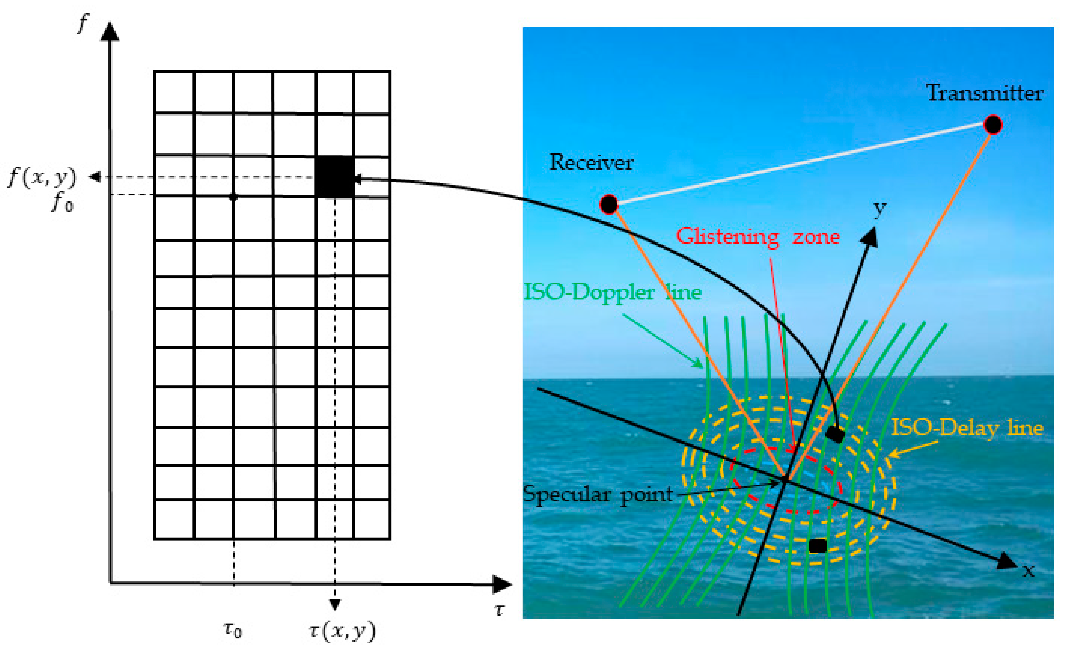
2.1. Spaceborne GNSS-R DDM and Delay Waveforms

GNSS reflected signals are composed of signals scattered by different scattering units, which have different time delay and doppler frequency. As shown in Figure 1, DDM not only represents the distribution of GNSS reflected signals in the time-delay doppler domain, but also represents the distribution of scattered energy in the spatial domain. Spatial domain and time-delay doppler domain do not have a one-to-one mapping relationship. There are two points of intersection between the iso-delay ellipse (e.g., yellow dotted ellipses in Figure 1) and the iso-Doppler line (e.g., the green hyperbolas). The adjacent iso-delay lines and the adjacent two iso-Doppler ellipses intersect in space to form two different physical regions—that is, the reflected power of two different physical regions on the sea surface corresponds to the same delay-Doppler region.

The power of scattered GNSS signals is a 2D function of time delay and doppler. For given time delay τ and doppler frequency shift f, the received signal power of scattered GNSS signals is the integral of the power distribution on the scattering surface. Zavorotny and Voronovich derived a model to describe received signal power of scattered (or reflected) signals [22], which is given by:

$$\langle {\left|Y(\tau ,f)\right|}^2\rangle =\frac{T_i^2{\lambda }^2{P}_t{G}_t}{{(4\pi )}^3}{\iint }\frac{G_r}{R_t^2{R}_r^2}{\Lambda }^2(\tau )sin{c}^2(f){\sigma }_{0}dA,$$

(1)

where $\langle {\left|Y(\tau ,f)\right|}^2\rangle$ is the reflected signal power at the receiver, which is a function of time delay $\tau$ and Doppler frequency shift $f$; $T_i$ is the coherent integration time; $\lambda$ denotes the signal wavelength; $P_t$ is the satellite transmitting power; $G_t$ is the satellite antenna gain; $G_r$ is the receiver antenna gain; $R_t$ and $R_r$ are distance from satellite transmitter and receiver to specular point of reflection, respectively. $\Lambda (\tau )$ is PRN code auto-correlation function, and $sinc(f)$ is the sin function describing doppler frequency shift induced power reduction. ${\sigma }_0$ refers to the scattering coefficient per unit area of surface A, namely NBRCS, which is related to the roughness of the scattering surface. In this work, NBRCS (${\sigma }_0$) was used as a surface roughness sensitivity parameter (also known as an observable parameter) to estimate sea surface wind speed. The NBRCS equation is given as follows [22,34,40]:

$${\sigma }_0(\overrightarrow{\ell })=\frac{\pi {\left|\Re (\overrightarrow{\ell })\right|}^2{q}_{}^4(\overrightarrow{\ell })}{q_z^4(\overrightarrow{\ell })}P\left(-\frac{q_{\perp }(\overrightarrow{\ell })}{q_z(\overrightarrow{\ell })}\right),$$

(2)

where ℜ is Fresnel reflection coefficient, whose calculation formula is shown in Equations (3)–(6) [22,41]; q is the scattering unit vector; q_z is the vertical component (surface normal direction); $q_{\perp }$ is the horizontal component of the scattering unit vector; $\ell$ is the vector from the specular point to the scattered point, and P is the probability density function (PDF).

$${\Re }_{RR}={\Re }_{LL}=\frac{1}{2}\left[{\Re }_{VV}+{\Re }_{HH}\right],$$

(3)

$${\Re }_{RL}={\Re }_{LR}=\frac{1}{2}\left[{\Re }_{VV}-{\Re }_{HH}\right],$$

(4)

$${\Re }_{VV}=\frac{\epsilon sin\theta -\sqrt{\epsilon -co{s}^2\theta }}{\epsilon sin\theta +\sqrt{\epsilon -co{s}^2\theta }},$$

(5)

$${\Re }_{HH}=\frac{sin\theta -\sqrt{\epsilon -co{s}^2\theta }}{sin\theta +\sqrt{\epsilon -co{s}^2\theta }}.$$

(6)

In the above, $\theta$ is the angle of incidence, and $\epsilon$ is the complex permittivity. $R$,$L$,$V$, and $H$ represent right-hand circular polarization (RHCP), left-hand circular polarization (LHCP), vertical polarization, and horizontal polarization, respectively. Let the permittivity of sea water be ${\epsilon }_{\mathrm{Water}}=73.42+56.07i$ [42], then we can derive the relation between the modulus of Fresnel reflection coefficient and the elevation angle as shown in Figure 2. It can be seen that the LHCP component of reflected signal increases with the increase in GNSS satellite elevation angle, while its RHCP component decreases with the increase in GNSS satellite elevation angle. The horizontal component of the reflected signal polarization decreases with the increase in the elevation angle of GNSS satellite, while its vertical component increases with the increase in the elevation angle. Note that the above trend only appears when the elevation angle is greater than a certain value (about 6.8 °). This indicates that after the incident RHCP GNSS satellite signal is scattered over the sea surface, its polarization characteristics will change—that is, the signal dominated by RHCP will change to that dominated by LHCP, and the energy ratio of conversion is relatively large.

Spaceborne GNSS-R can be regarded as a bistatic radar scatterometer. In order to illustrate the power of the scattered GNSS signals, a theoretical integral delay waveform (IDW) model is proposed in [22,25], shown as follows:

$$W_I(\tau )=\frac{1}{N}{\displaystyle \sum _{i=1}^N\langle {\left|Y_{\mathrm{incoh}}(\tau ,f_i)\right|}^2\rangle },$$

(7)

where $W_I(\tau )$ is the IDW, which is obtained by accumulating the time delay waveform corresponding to all doppler frequency shift values. $\langle {\left|Y_{\mathrm{incoh}}(\tau ,f_i)\right|}^2\rangle$ is the scattered power value minus the noise floor, at the delay and Doppler coordinates $\tau$ and $f_i$.

For CYGNSS, $N_{\tau }=17$,$N_f=11$ and the Doppler bandwidth $\Delta f=1/2T_i=500$ Hz. It can be seen from [22,43] that when the width of the glistening zone is smaller than the Doppler bandwidth, the influence of Doppler effect can be ignored. At this point, a central delay waveform (CDW) without Doppler frequency shift can be obtained as follows:

$$W_C(\tau )=T_i^2{\displaystyle \mathsf{\int }\frac{L^2(\overrightarrow{\ell })}{4\pi R_t^2(\overrightarrow{\ell })R_r^2(\overrightarrow{\ell })}}{\left|\Lambda (\tau -(R_t(\overrightarrow{\ell })+R_r(\overrightarrow{\ell }))\right|}^2{\sigma }_0(\overrightarrow{\ell })d^2\ell ,$$

(8)

where most of the terms are the same as those in Equations (1) and (2), and $L^2$ is the function of power antenna footprint.

When IDW and CDW are normalized, respectively, the normalized multi-delay waveform (NIDW) and the normalized central delay waveform (NCDW) can be obtained, as shown in Equations (9) and (10):

$$W_I^{Normalized}=W_I(\tau )/W_I^{max},$$

(9)

$$W_C^{Normalized}=W_C(\tau )/W_C^{max},$$

(10)

where $W_I^{max}$ and $W_C^{max}$ represent the maximum values of IDW and CDW before normalization, respectively. Differential delay waveform (DDW) can be obtained by differentiating between NIDW and NCDW, shown as follows:

$$W_D(\tau )=W_I^{Normalized}(\tau )-W_C^{Normalized}(\tau ).$$

(11)

In the retrieval of sea surface wind speed, the power values of time-delay 1D correlation function (also called time-delay waveform) are closely related to the physical parameters such as sea surface wind speed and wind direction. Figure 3a–d show the DDM maps under different wind speed conditions, and Figure 3e–g present the corresponding delay waveform. It can be seen that the time delay waveform of reflected signal has different characteristics under different wind speed conditions. In view of this, the time delay waveform is used as the basic observations to retrieve wind speed in our study. See Section 2.2 and Section 3.2 below for details.

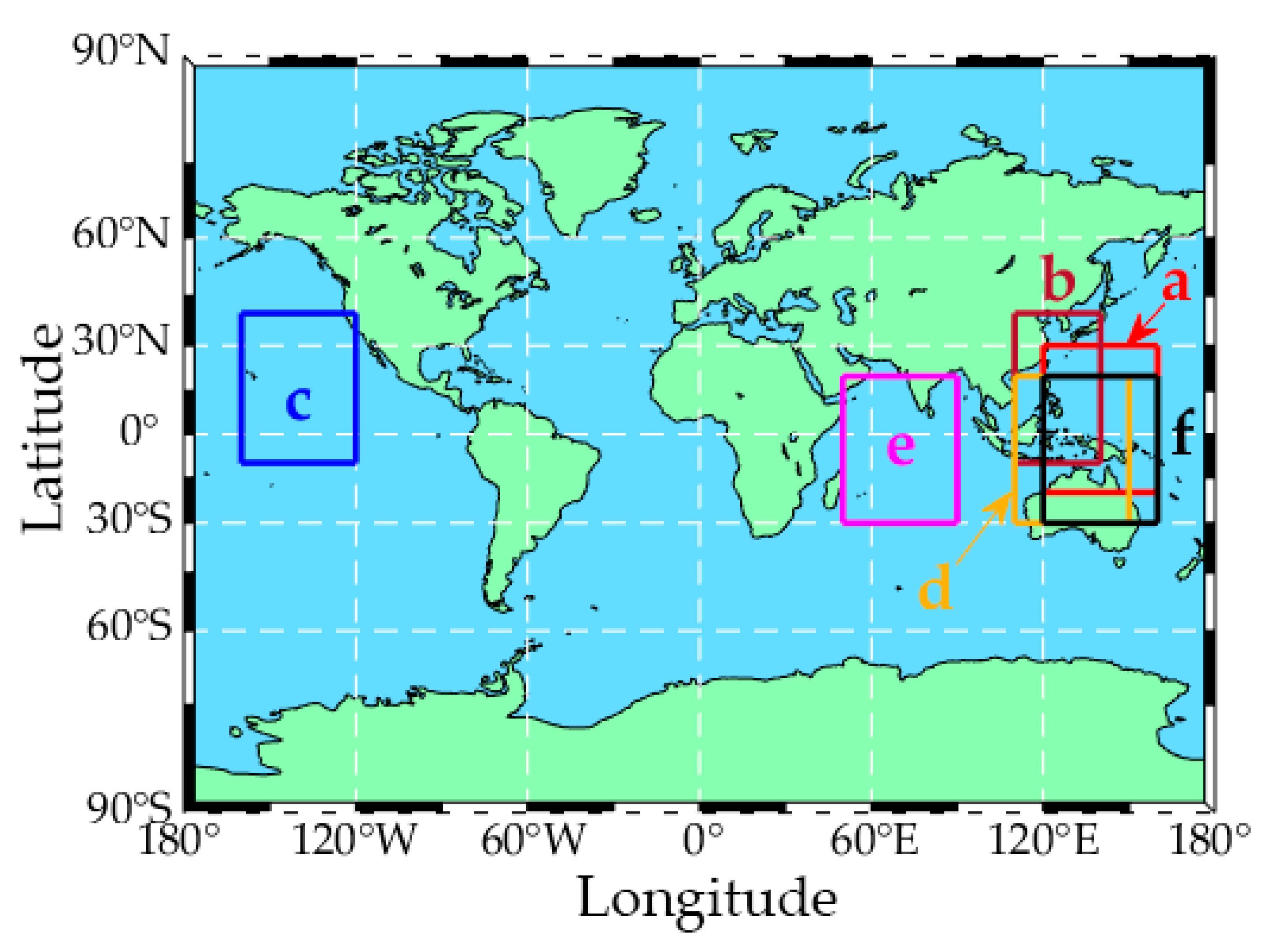
2.2. Data Set

In order to derive sea surface wind speed from DDM and delay waveform, we, respectively, adopt the methods of NBRCS, delay waveform LES, and optimal weight eigenvalue combination to construct GMF. We introduce two data sets, namely CYGNSS L1 DDM data and European Centre for Medium-Range Weather Forecasts (ECMWF) reanalysis data.

In 2016, the CYGNSS was deployed, which was developed by NASA, the University of Michigan, and the Southwest Research Institute. It consists of 8 microsatellites, with an orbital inclination of 35°, a height of 510 km, and a spatial resolution of 25 × 25 km [44]. Delay doppler mapping instrument (DDMI) [45] is equipped onboard each CYGNSS satellite, which is specially used for GNSS reflectometry. The CYGNSS products mainly include four levels of products, namely, level 1, level 2, level 3, and level 4. The first three levels of products are open to the public, and now available in NASA’s Physical Oceanography Distributed Active Archive Center (PO. DAAC) on (https://podaac.jpl.nasa.gov/) [46], with the data being in NetCDF format. In our wind speed retrieval, we use level 1 V2.1 product, downloaded from the website (https://podaac-tools.jpl.nasa.gov/drive/files/allData/cygnss/L1/v2.1). We downloaded the observation data from 12 May 2020 to 12 August 2020, with day-of-year ranging from 133 to 225.

The latest ECMWF data, called ERA5, can be downloaded from Copernicus climate change service (C3S) climate database (https://cds.climate.copernicus.eu/cdsapp#!/home). ERA5 provides hourly information on the atmosphere, land surface, and ocean waves from 1979 to the present. The spatial resolution of wind speed products is 0.5° × 0.5°, and there are two data formats: GRIB and NetCDF. For long-term large-scale observations of sea surface wind speed, the current wind speed product of ECMWF can be used as the ground-truth data in CYGNSS wind speed retrieval. ECMWF assimilates meteorological data from different sources and obtains an ERA-5 reanalysis data set containing wind speed of 10 m above the sea surface. Therefore, NBRCS and LES of IDW calculated from CYGNSS DDM data are matched with wind speed of ECMWF reanalysis data, respectively, to develop an empirical geophysical function model.

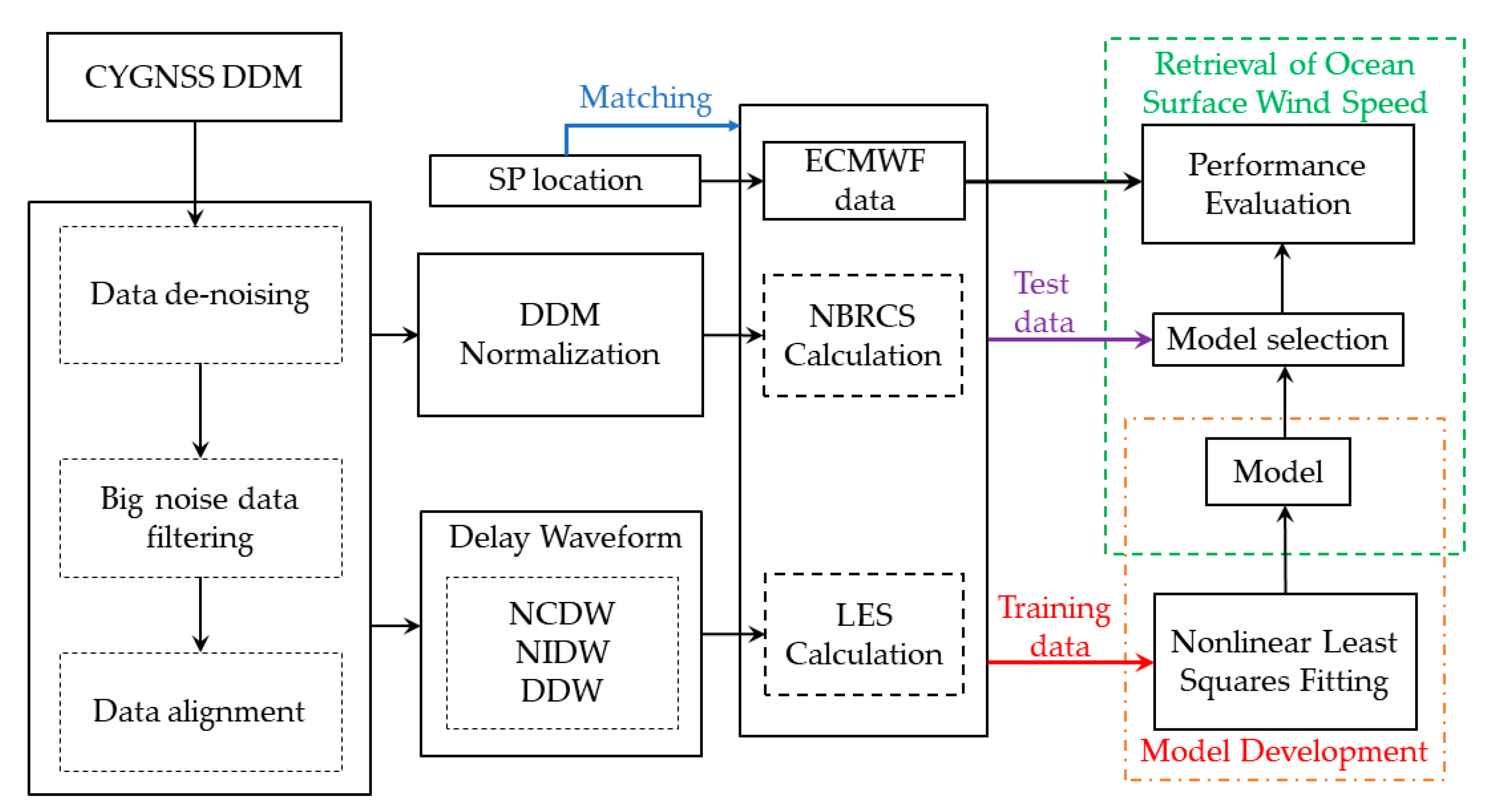
2.3. Methodology

In order to obtain accurate wind speed retrieval results, a series of processing work was performed for the selected data sets. Data preprocessing is necessary to improve the efficiency of subsequent data processing and the reliability of the algorithm. This section mainly deals with data preprocessing, with a focus on data filtering and DDM data alignment. We proposed a data filtering method based on threshold setting for data quality control.

First, the method described in [47,48] was used to reduce the noise in the noisy DDM data. Since the initially denoised DDM data usually contain significant noise, it is necessary to select better quality data from the initially denoised DDM data. The traditional selection method generally uses the SNR peak as the index of data filtering. For example, in [26], the threshold of SNR peak is set to 0 dB, and the DDMs with SNR peak greater than the threshold are selected; in [29,49], the SNR peak threshold is set to 3 and 4 dB, respectively. Although the above SNR peak method can be effectively used for DDM selection, there are some deficiencies in threshold selection. If the selected threshold is too large, good quality data may be lost, while if the selected threshold is too small, noise data cannot be well excluded, resulting in performance degradation. In view of this, in [43], a DDM selection method based on differential time-delay waveform was proposed. The RMSE of 0.5 of differential delay waveform was set as the threshold, which is employed in our data selection method. We use DDM data of CYGNSS L1 level, which is composed of 17 time-delay rows and 11 doppler columns of data. Since the differential data were used, [43] is not completely applicable to the data adopted in this paper, so in the data filtering process, the calculation of IDW has a slight improvement in the processing method, as shown in Equation (12).

$$W_I^{Normalized}={\displaystyle \sum _{i=4}^8{P}_r({\tau }_{}^{row},f_i^{col})}.$$

(12)

Figure 4 shows a map of DDM (Figure 4a) of CYGNSS and its corresponding delay waveforms (NIDW, NCDW, and DDW, Figure 4b). We mainly selected the grids corresponding to the 17 time-delay rows and the 4–8th Doppler-shift columns in the DDM data to be accumulated and calculated to obtain IDW and then normalized. Then, we calculated the difference between NIDW and NCDW to obtain the differential delay waveform (DDW).

Figure 5 shows the two DDMs in the presence of large noise (Figure 5a) and small noise (Figure 5b) and the corresponding delay waveforms. Both DDM data were recorded over the ocean on 12 May 2020. As shown in Figure 5, in the presence of large noise (low SNR = 0.5207 dB), significant variation and dispersion occurred in different time-delay waveform, while in the presence of small noise (high SNR = 2.6943 dB), the variation in the differential waveform was much smaller. Large noise may be caused by the space environment of signal propagation, such as atmospheric attenuation, space signal interference, and propagation loss. Data quality is also affected by incident angle, antenna gain, and satellite attitude. After denoising the DDM data, we calculated the RMS values of DDW, as shown in Equation (13). We selected good-quality DDM data by adjusting the root mean square (RMS) threshold of cleaned DDW.

$$RM{S}_{DDW}=\sqrt{\frac{1}{q}{\displaystyle \sum _{p=1}^q{(DD{W}_p)}^2}},$$

(13)

where $RM{S}_{DDW}$ represents the RMS of DDW, and $DD{W}_p$ denotes the waveform value corresponding to each time-delay value.

We selected 4767 DDM data and calculated the RMS of DDW using formula (15) as shown in Figure 6. The results show that when the threshold is set as RMS = 0.25, about 88.15% DDWs can be selected; when the threshold is set as RMS = 0.2, about 92.96% DDWs can be selected; when the threshold is set as RMS = 0.1, about 95.51% DDWs can be selected. Considering both data utilization and data quality, in our study, DDW data with RMS greater than 0.2 were considered to contain large noise and thus excluded.

Now, it comes to the last step of data preprocessing. We use the alignment algorithm to align DDM data with time delay and Doppler zero values as reference. In this data matching stage, the obtained high-quality DDM data and delay waveforms are used to calculate NBRCS and LES of DDW, respectively. After that, they are matched with ECMWF data, respectively, and the DDM data are randomly divided into training data set and test data set according to the proportion of 70% and 30%, respectively. In the third stage (model development, model selection, and performance evaluation), the model is first developed using training data, selected characteristic parameters (NBRCS, LES), and curve fitting methods (such as nonlinear least square fitting). Then, the proposed empirical model is applied to the test data to obtain the sea surface wind speed estimate and evaluate the performance of different models. The flow chart of wind speed estimation model construction is shown in Figure 7.

3. Wind Speed Estimation Model

In this section, ECMWF reanalysis data from 12 May 2020 to 12 August 2020 are used as training and test data sets to derive wind speed estimation models. The reanalysis data provide a spatially continuous wider range of wind speeds and correspond to a large number of data sets. We developed new empirical models for sea surface wind speed estimation by using NBRCS, LES, and the combination of NBRCS and LES observations, respectively.

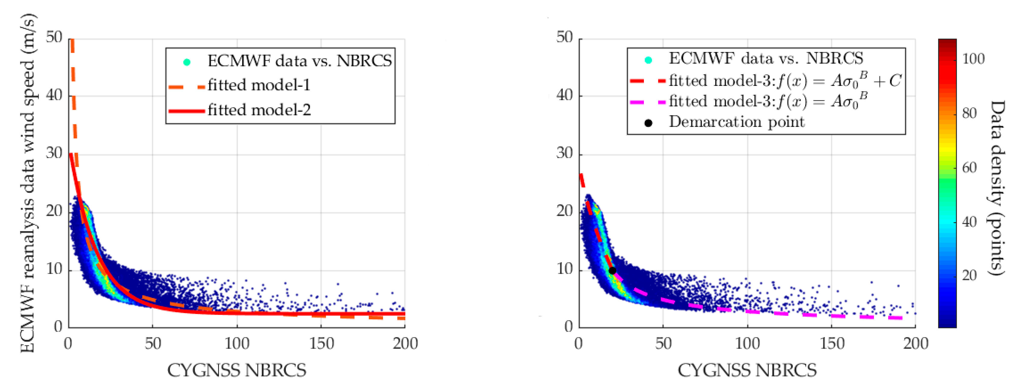
3.1. Modelling Using NBRCS Methods

We first selected the preprocessed DDM data to calculate NBRCS, and then matched the NBRCS with ECMWF data. We selected 70 % of the data for modeling. However, the spatial, temporal resolution of ECMWF reanalysis data was 0.5° × 0.5°, 1 h [50], while the spatial, temporal resolution of NBRCS was about 0.082° × 0.082° and 0.5 s. Considering these differences, we used the biharmonic spline interpolation (also called V4 interpolation) to combine them into DDM data with the spatial resolution being 0.1° × 0.1°, and the alignment criterion was 1 h.

3.1.1. NBRCS Calculation

In order to calculate NBRCS (${\sigma }_0$), the Equation (1) can be rewritten as follows [29]:

$$NBRCS=\frac{P_{DDM}{(4\pi )}^3{R}_T^2{R}_R^2}{{\lambda }^2{P}_T{G}_T}\mathsf{\iint }{\Lambda }^2(\tau )sin{c}^2(f)dA,$$

(14)

where $P_{DDM}$ is the power calibration result of $\langle {\left|Y(\tau ,f)\right|}^2\rangle$,$\langle {\left|Y(\tau ,f)\right|}^2\rangle$ is derived from Equation (1), and other definitions are consistent with Equation (1). It should be noted that the double integral in Equation (14) is determined only by the geometry. NBRCS has good accuracy only near specular reflection points. Therefore, up to 0.75 delay chips and 2500 Hz Doppler shifts were selected to calculate NBRCS.

3.1.2. Model-1, Model-2, and Model-3

We developed three empirical models of double-parameter (denoted as Model-1), triple-parameter (denoted as Model-2), and piecewise functions (denoted as Model-3), respectively.

Model-1 and Model-2 are derived from the training data in this paper, while the piecewise function in Model-3 is modified on the basis of [26,29]. They are expressed as follows:

Model-1:

$$f({\sigma }_0)=A{\sigma }_0{}^B,0<{\sigma }_0\le 200,$$

(15)

Model-2:

$$f({\sigma }_0)=A\exp (B{\sigma }_0)+C,$$

(16)

Model-3:

$$f({\sigma }_0)=\{\begin{array}{l}A{\sigma }_0{}^B+C,\mathrm{if}0<{\sigma }_0\le 20\\ A{\sigma }_0{}^B,\mathrm{if}20<{\sigma }_0\le 200\end{array},$$

(17)

where $f({\sigma }_0)$ is the wind speed estimated by the model; ${\sigma }_0$ is NBRCS; A, B, and C are unknown parameters, which are determined by fitting the training data set.

As shown in Figure 8, there is a functional relationship between NBRCS and true wind speed, which can be described by Model-1, Model-2, and Model-3. Using nonlinear least squares fitting method, Model-1 and Model-2 are obtained, which are shown in Figure 8 (left) as dotted lines and solid red lines, respectively. Model-3, constructed by piecewise functions, is shown in Figure 8 (right) as a red dotted line and a purple dotted line. The black points in the Figure 8 (right) are function demarcation points. That is, when NBRCS is in the range of 0~20, a power function with three arguments ($f({\sigma }_0)=A{\sigma }_0{}^B+C$) is used to retrieve wind speed, and when NBRCS is in the range of 20~200, a power function with two arguments ($f({\sigma }_0)=A{\sigma }_0{}^B$) is used to retrieve wind speed. This takes into account the fitting effect of high wind speed and low wind speed separately. The fitting parameters of the three models are given in

Table 1. Fitting parameters of Model-1, Model-2, and Model-3.

Models	A	B	C
Model-1	98.0506	−0.7641
Model-2	30.2831	−0.0615	2.5
Model-3 Function 1	−2.8648	0.6495	29.9137
Model-3 Function 2	205.2	−1.043

.

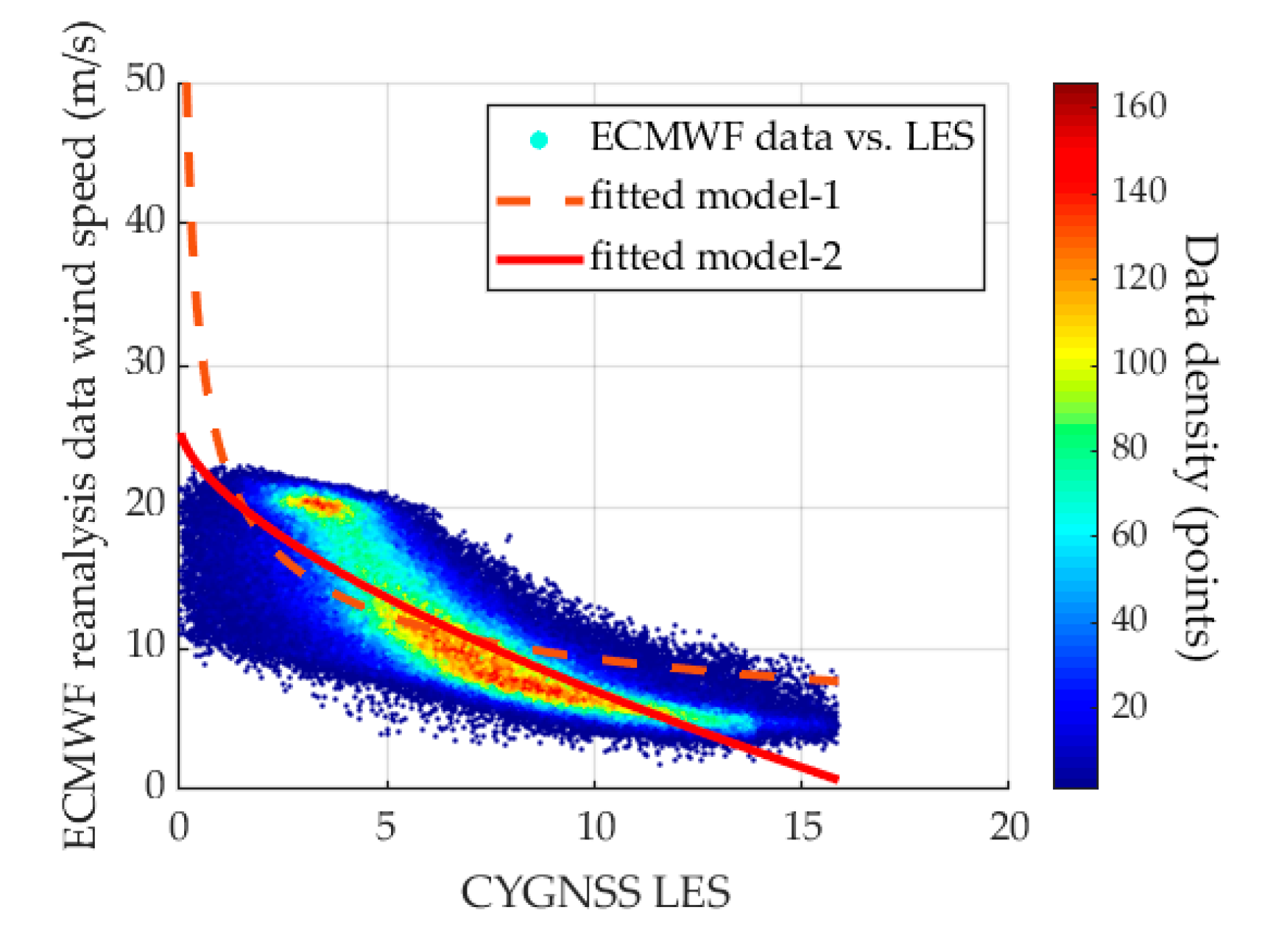
3.2. Modelling Using LES Methods

Using the same process as in Section 3.1, we first selected the preprocessed DDM data to calculate LES and matched LES with ECMWF data. Then, we selected 70 % of the data for modeling, while the remaining 30 % was used to test model performance.

3.2.1. LES Calculation

The least squares fitting is usually used to calculate the slope of multiple points. The calculation is expressed as Equation (18).

$$LE{S}_n=\frac{{\displaystyle \sum _{i=1}^n{\tau }_i{W}_i^{LES}-n\overline{\tau }\overline{W^{LES}}}}{{\displaystyle \sum _{i=1}^n{\tau }_i{}^2-n{(\overline{\tau })}^2}},$$

(18)

where n (n ≥ 2) denotes the number of the selected points used in the slope fitting, and ${\tau }_i$ represents the abscissa value of each point used in fitting the leading edge slope, namely the time delay values. $W_i^{LES}$ is the ordinate value, namely the leading edge waveform value. $\overline{\tau }$ and $\overline{W^{LES}}$ are the average of the abscissa value and that of the ordinate value.

In this paper, LES is defined as the slope of the leading edge of the IDW. In other words, after incoherent accumulation of DDM corresponding to Doppler frequency within a certain range to obtain one-dimensional delay waveform, the least squares fitting is adopted to obtain the optimal slope of the function, which is the leading edge slope of this delay waveform.

3.2.2. Model-1 and Model-2

As shown in Figure 9, the model trained by LES and ECMWF reanalysis data follows the form of power function. We developed the double-parameter Model-1 and triple-parameter Model-2, respectively. When the determination coefficient between the fitted wind speed and the true wind speed is close to 1 and the RMSE is the smallest, the fitting model is optimal. The dashed curve is the best fitting function of Model-1, and the red curve is the best fitting function of Model-2. The model formulas are described as follows:

Model-1:

$$F(x_{LES})=G{x}_{LES}{}^M,x_{LES}\in \mathrm{R},$$

(19)

Model-2:

$$F(x_{LES})=G{x}_{LES}{}^M+L,x_{LES}\in \mathrm{R},$$

(20)

where $F(x_{LES})$ is the estimated wind speed; $x_{LES}$ is LES; G, M, and L are undetermined parameters, which are obtained by fitting the training data set.

3.3. Modeling Using Determination Coefficient-Based Combination

The solution of fitting parameters is an optimization problem, and we use the minimum mean square error (MSE) criterion to achieve the goal. In other words, taking the comparison data as the ideal truth value, we found that the MSE between the retrieval results and the comparison data is minimized.

Suppose that the estimated value of wind speed is $\widehat{x}$, and the true value of wind speed is $y$. due to the randomness of $\widehat{x}$, the MSE can be expressed statistically by the following equation:

$$MSE(\widehat{x})=E{(\widehat{x}-y)}^2,$$

(21)

$$MSE(\widehat{x})=E{(\widehat{x}-E(\widehat{x}))}^2+E{[E(\widehat{x})-y]}^2+2E\{[\widehat{x}-E(\widehat{x})][E(\widehat{x})-y]\},$$

(22)

$$MSE(\widehat{x})=\sigma {(\widehat{x})}^2+{[E(\widehat{x})-y]}^2,$$

(23)

It can be seen that the MSE consists of variance ($\sigma {(\widehat{x})}^2$) and square of deviation (${[E(\widehat{x})-y]}^2$). When $\widehat{x}$ is the unbiased estimation of $y$, the MSE is reduced to variance, and the uniformly minimum mean square error estimation is the uniformly minimum variance unbiased estimation.

Under the minimum mean square error criterion, we exploit the determination coefficient to measure the actual performance of a model and use it as the optimization index in fitting. The equation is as follows:

$$R^2=1-\frac{{\displaystyle \sum _{i=1}^m{(y_i-y_{model,i})}^2}}{{\displaystyle \sum _{i=1}^m{(y_i-{\overline{y}}_i)}^2}},$$

(24)

where R² is the determination coefficient, $y_i$, and ${\overline{y}}_i$ are the wind speed and average wind speed of ECMWF data, respectively. $y_{model,i}$ is the wind speed of the fitting model.

Based on the minimum MSE criterion, by calculating the determination coefficient of the constructed model in Section 3.1 and Section 3.2, we found that the fitting result of Model-3 was better than that of the other two models (Model-1 and Model-2) when the NBRCS method was used to construct the model. When the LES method was used to construct the model, the fitting result of Model-2 was better than that of Model-1. In view of this, the combination model was established by using the determination coefficient of Model-3 in the NBRCS method and that of Model-2 in LES method. In other words, the wind estimates of NBRCS and LES methods were linearly combined into a best weighted estimator, using determination coefficient. Here, the combination model based on determination coefficient (CMDC) is defined as follows:

$$U_{Model}=\frac{{\kappa }_1·y_i^{{\mathrm{NBRCS}}_{[Model-3]}}+{\kappa }_2·y_i^{LE{S}_{[Model-2]}}}{{\kappa }_1+{\kappa }_2},$$

(25)

$$\{\begin{array}{l}{\kappa }_1=1-\frac{{\displaystyle \sum _{i=1}^n(y_i^{obs}}-y_i^{{\mathrm{NBRCS}}_{[Model-3]}}{)}^2}{{\displaystyle \sum _{i=1}^n(y_i^{obs}}-\overline{y_i^{obs}}{)}^2},\\ {\kappa }_2=1-\frac{{\displaystyle \sum _{i=1}^n(y_i^{obs}}-y_i^{LE{S}_{[Model-2]}}{)}^2}{{\displaystyle \sum _{i=1}^n(y_i^{obs}}-\overline{y_i^{obs}}{)}^2},\end{array}$$

(26)

where $U_{Model}$ is a CMDC-based wind speed estimate, ${\kappa }_1$ and ${\kappa }_2$ are weights, $y_i^{{\mathrm{NCBRS}}_{[Model-3]}}$ is the estimated wind speed of Model-3 in NBRCS method, $y_i^{LE{S}_{[Model-2]}}$ is the estimated wind speed of Model-2 in LES method, $y_i^{obs}$ and $\overline{y_i^{obs}}$ are the wind speed and average wind speed of ECMWF data, respectively. n is the number of observations.

4. Results and Performance Evaluation of Retrieving Wind Speed

This section uses the remaining 30 % test data to verify the performance of the empirical wind speed estimation models deduced above. As shown in Figure 10, some of the remaining test data are mainly distributed in the range of 50°~160°E, 30°S~40°N and 160°~120°W, 10°S~40°N. Regions a, b, c, d, e, and f in Figure 10 correspond to sub-graphs (a), (b), (c), (d), (e), and (f) in Figure 11, respectively, and are mainly in the Pacific and Indian Oceans.

4.1. Assessment Method

In order to verify the performance of the wind speed estimation model, the estimated wind speed was compared with ERA-5 reanalysis data of ECMWF. RMSE, mean absolute error (MAE), Pearson correlation coefficient, and mean absolute percentage error (MAPE) were used to evaluate the performance of wind speed estimated by the models [51]. Their calculation formulas are as follows:

$$RMSE(h)=\sqrt{\frac{1}{m}{\displaystyle \sum _{i=1}^m{(h_i-y_i)}^2}},$$

(27)

$$MAE(h)=\frac{1}{m}{\displaystyle \sum _{i=1}^m\left|h_i-y_i\right|},$$

(28)

$$R=\frac{{\displaystyle \sum _{i=1}^m(h_i-{\overline{h}}_i)(y_i-{\overline{y}}_i)}}{\sqrt{{\displaystyle \sum _{i=1}^m(h_i-{\overline{h}}_i){)}^2{\displaystyle \sum _{i=1}^m{(y_i-{\overline{y}}_i)}^2}}}},$$

(29)

$$MAPE=\frac{1}{m}{\displaystyle \sum _{i=1}^m\left|\frac{h_i-y_i}{y_i}\right|}\times 100\%,$$

(30)

where m is the number of samples, $h_i$ is the estimated wind speed, ${\overline{h}}_i$ is the mean of $h_i$, $y_i$ is the wind speed derived from ERA-5 reanalysis data, and ${\overline{y}}_i$ is the average of $y_i$.

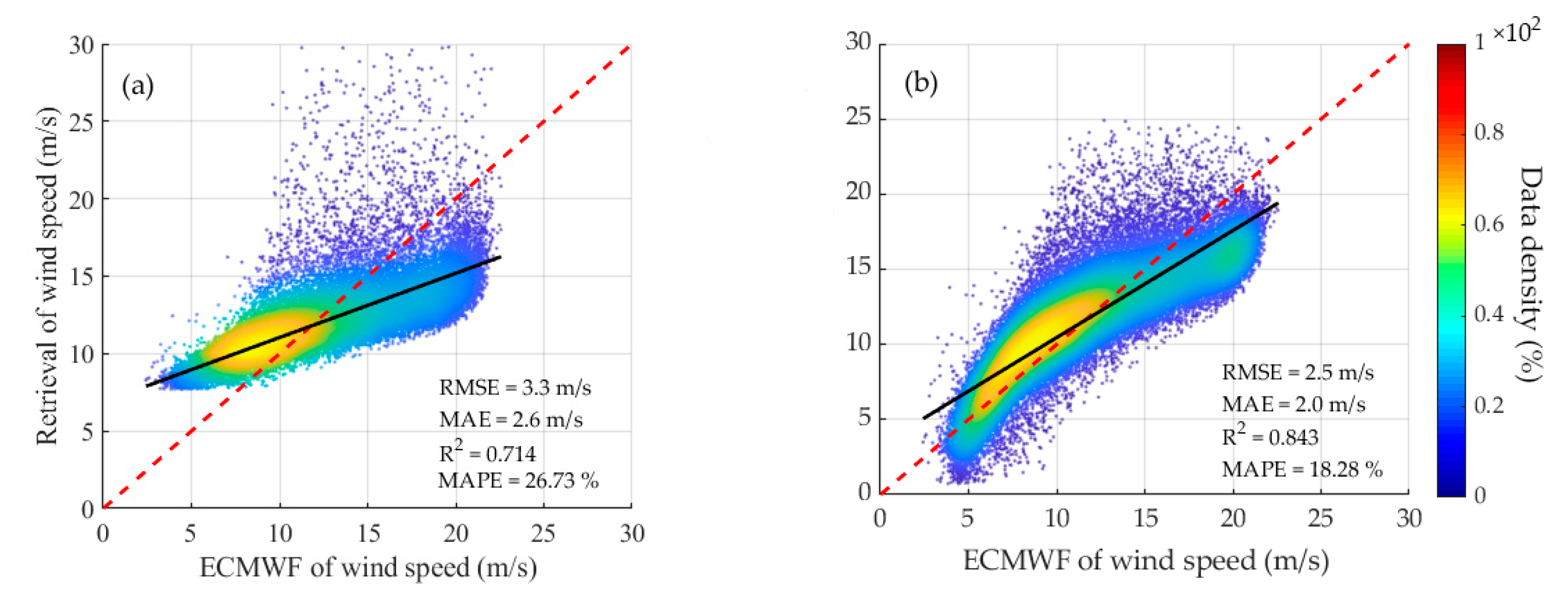
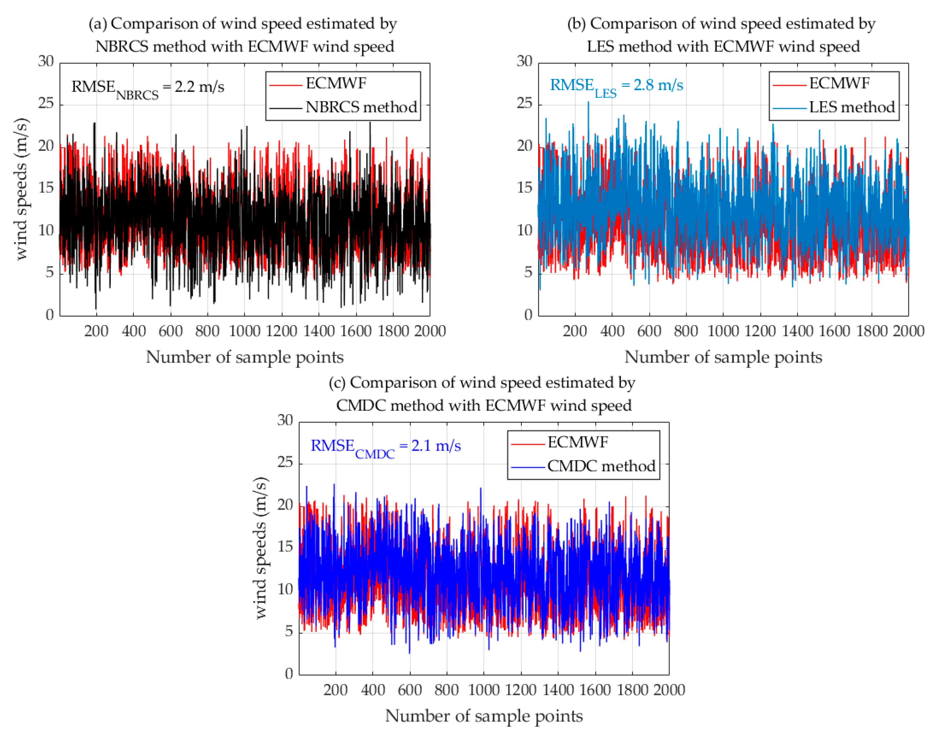
4.2. Performance Assessment of wind Speed Estimation Model Based on NBRCS Method with Double Parameters (Model-1), Triple Parameters (Model-2), and Piecewise Function (Model-3)

In this section, we first selected the data pairs for 6 days in the test data set, and then compared the wind speed estimated by the models with the ECMWF reanalysis wind speed. See Figure 12 for statistical results. The wind speed estimation values were shifted by the same amount to avoid overlapping. From Figure 12, we can observe that the accuracy of the estimated wind speed of Model-3 was better than that of Model-1 and Model-2. For example, during the observation period 20,200,710 02:00–02:30, the wind speed estimation accuracy of Model-3 was 0.9 m/s, which is 56.49 % and 57.21% better than that of Model-1 and Model-2, respectively. The estimation accuracy of Model-3 was 1.8 m/s (in the time period of 20,200,723 14:00–14:30), which means that the accuracy improved by 10.0% and 28.0%, respectively, compared with Model-1 and Model-2. From the 6-day wind speed estimation results, the average RMSE of Model-1, Model-2, and Model-3 was 1.9, 2.4, and 1.3 m/s, respectively. The wind speed estimation accuracy of Model-3 was about 31.58% and 45.83% higher than that of Model-1 and Model-2.

Then, correlation analysis was conducted between the model’s estimated wind speed and the ECMWF’s ERA-5 reanalysis data. Figure 13 shows the scatter plot of the estimated wind speed of Model-1, Model-2, and Model-3 and the ECMWF wind speed, respectively. RMSE, MAE, R², and MAPE are marked in Figure 12a. The RMSE, MAE, and MAPE of the estimated wind speed using Model-1 were 2.6 m/s, 2.0 m/s, and 18.65 %, respectively, and the coefficient of determination R² was 0.836. As shown in Figure 12b, the RMSE, MAE, and MAPE of the estimated wind speed using Model-2 were 2.7 m/s, 2.2 m/s, and 22.42 %, and the coefficient of determination R² was 0.876, respectively. In Figure 12c, the RMSE, MAE, and MAPE of the estimated wind speed using Model-3 were 2.3 m/s, 1.9 m/s, and 18.43 %, respectively, and the coefficient of determination R² was 0.881.

To sum up, whether from the perspective of a single day and/or a certain period of time wind speed estimation results, or from the general (the remaining 30%) test data of wind speed estimation results, Model-3 achieved the best wind speed estimation performance among the three models, which illustrates that the construction of Model-3 to estimate the wind speed has the best feasibility, applicability, and robustness. However, in the case of high wind speed (the wind speed is greater than 20 m/s), the wind speed estimation errors became larger for the three models generally, but Model-3 had a certain improvement compared with the other two models. The error sources of the model estimation of wind speed mainly include: (1) The time resolutions of CYGNSS and ECMWF reanalysis data are not exactly the same. The matching of some sample instants is based on a close approximation of time, which may lead to differences in wind speed. (2) ERA-5 is reanalysis data absorbing a large amount of historical data from different sources, which have some errors and uncertainty as well [44].

4.3. Double-Parameter (Model-1) and Triple-Parameter (Model-2) Performance Assessment Based on LES Observations

As described in Section 4.2, we first selected data pairs for 6 days in the test data set, and then compared the estimated wind speed with ECMWF reanalysis wind speed. The statistics results are presented in Figure 14. The wind speed estimation values were shifted by the same amount to avoid overlapping. We can observe that the performance of the triple-parameter Model (Model-2) constructed in LES method was better than that of the double-parameter Model (Model-1), and Model-2 had good robustness. The average RMSE of Model-1 and Model-2 was 2.6 and 1.9 m/s, respectively, and the wind speed estimation accuracy of Model-2 was about 26.92% higher than that of Model-1. Then, the model developed by the LES method was used to estimate the wind speed and analyze the correlation between ECMWF ERA-5 reanalysis data. Figure 15 shows the scatter plots of Model-1- and Model-2-based wind speed estimates versus ECMWF wind speed, respectively. RMSE, MAE, R², and MAPE are marked in Figure 15. As shown in Figure 15a, the RMSE, MAE, and MAPE of Model-1 estimated wind speed were 3.3, 2.7, and 26.73%, respectively, and the coefficient of determination R² was 0.714. As shown in Figure 15b, the RMSE, MAE, and MAPE of Model-2-based wind speed estimation were 2.5, 2.0, and 18.28%, respectively, and the coefficient of determination R² was 0.843.

To sum up, the performance of Model-2 was better than Model-1 in wind speed estimation. Different models have a great impact on wind speed estimation accuracy, especially under high wind speed cases (wind speed greater than 20 m/s), where the error of wind speed estimation is larger. However, compared with Model-1, Model-2 showed some improvement, with an accuracy increase of about 24.24%.

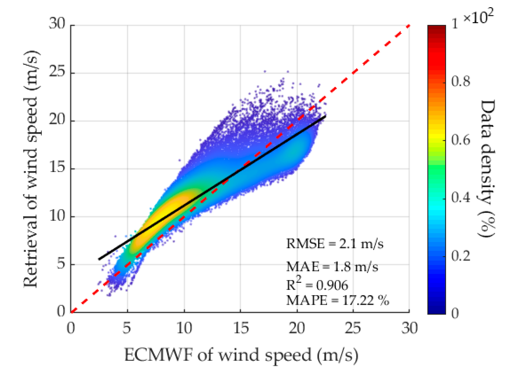
4.4. Performance Assessment of the Combination Model Based on Determination Coefficient (CMDC)

Based on the construction of wind speed estimation model by NBRCS and LES, a CMDC method is proposed to achieve a performance gain as described earlier. As shown in Figure 16, 2000 sampling points were randomly selected in the remaining 30% test data set to compare the wind speed estimated by CMDC method, Model-3 in NBRCS method, and Model-2 in LES method with the ECMWF wind speed. It can be seen that the RMSE value of CMDC method was lower than that of Model-3 in NBRCS method and Model-2 in LES method. Figure 17 shows the scatter plot of CMDC estimation of wind speed and ECMWF wind speed,

Table 2. The RMSE, MAE, R², and MAPE of wind speed estimated by NBRCS, LES, and CMDC methods (the sixth column is the accuracy improvement of the CMDC method compared with the other two methods).

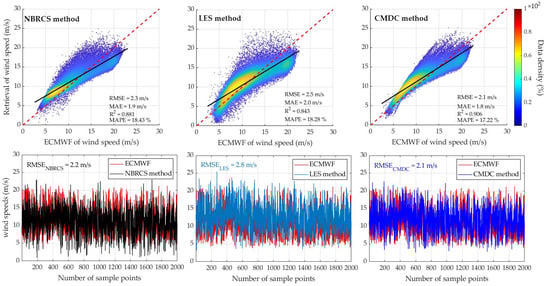
Methods	RMSE (m/s)	MAE (m/s)	R2	MAPE (%)	Improvement (%)
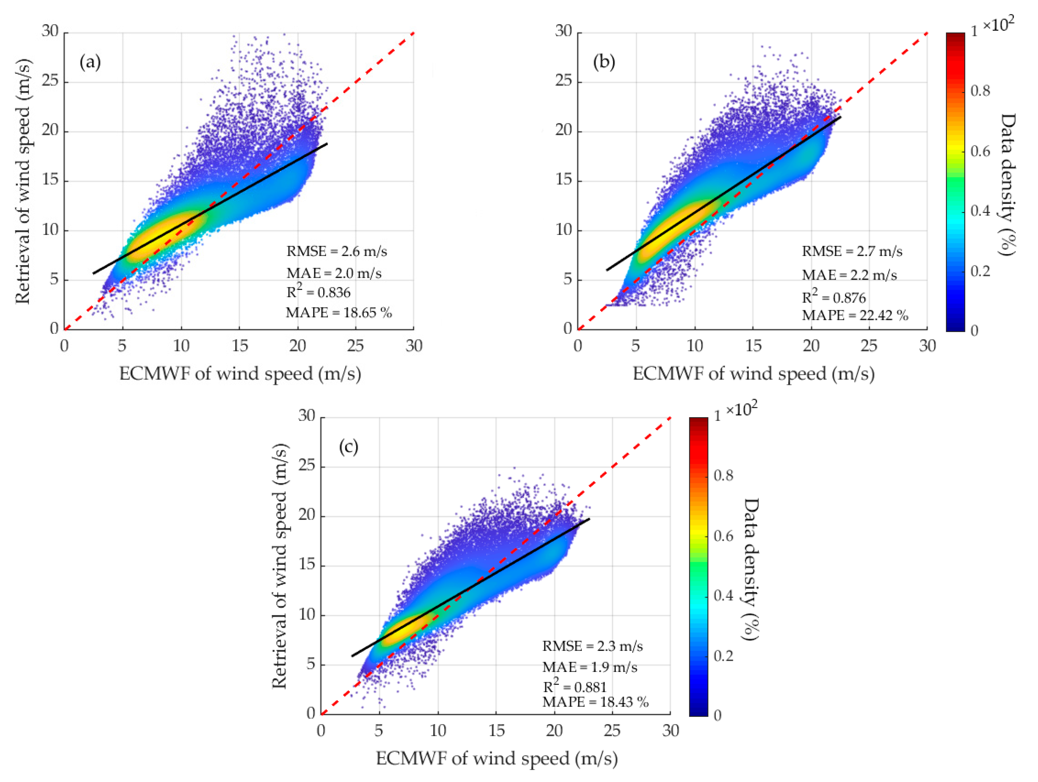
NBRCS method	2.3	1.9	0.881	18.43	8.69
LES method	2.5	2.0	0.843	18.28	16.0
CMDC method	2.1	1.8	0.906	17.22

shows the RMSE, MAE, R2, and MAPE of wind speed estimated by NBRCS, LES, and CMDC methods. As shown in Figure 17 and Table 2, from the comparison of wind speed estimated by the CMDC method with ECMWF wind speed for the 30% test data set, the RMSE of the estimated wind speed was 2.1 m/s, and the coefficient of determination R² was 0.906, which improved by 8.69% compared with Model-3 in NBRCS method, and by 16.0% compared with that of Model-2 in the LES method.

In order to perform a differentiated analysis for low and high wind speed regimes,

Table 3. The RMSE, MAE, and MAPE of wind speed estimated by NBRCS, LES, and CMDC methods (the wind speed is below and above 15 m/s).

Methods	<15 m/s			>15 m/s
	RMSE (m/s)	MAE (m/s)	MAPE (%)	RMSE (m/s)	MAE (m/s)	MAPE (%)
NBRCS method	1.6	1.5	11.5	2.6	1.9	16.9
LES method	1.8	1.6	14.4	3.2	2.4	18.8
CMDC method	1.5	1.3	9.1	2.3	1.6	14.7

shows the results of wind speed estimation by the three models against ECMWF reanalysis wind speed data when the wind speed is below and above 15 m/s. We can see from Table 3 that when the wind speed was less than 15 m/s, the RMSE, MAE, and MAPE of the wind speed estimation by the CMDC method were 1.5 m/s, 1.3 m/s, and 9.1%, respectively, compared with NBRCS and LES methods. The accuracy of the wind speed estimation improved by 6.3% and 16.7%, respectively. When the wind speed was greater than 15 m/s, the RMSE, MAE, and MAPE of the CMDC method were 2.3 m/s, 1.6 m/s, and 14.7%, respectively, and the wind speed estimation accuracy improved by 11.5% and 28.1%, respectively. Compared with NBRCS and LES methods, the combined model showed good performance enhancement. The results show that the wind speed estimation accuracy of the three models was higher when the wind speed was lower than 15 m/s, but it was lower when the wind speed was greater than 15 m/s. Despite all this, when the wind speed was greater than 15 m/s, the RMSE, MAE, and MAPE of wind speed estimation by the CMDC method were 2.3 m/s, 1.6 m/s, and 14.7%, respectively.

4.5. Discussion

As mentioned above, in the wind speed estimation based on GNSS-R, if the DDM data with large observation noise are not eliminated, the accuracy of wind speed inversion will be degraded. Therefore, we first proposed a data filtering method based on threshold setting for data quality control. This method can select good-quality DDM data by adjusting the root mean square (RMS) threshold of cleaned DDW. Then, five models were developed using observations, and a fusion-based model was also developed by combining the results of two models. In the model test phase, we compared the wind speed estimations of different models with the reanalysis wind speed data of ECMWF. Wind speed was divided into two regions, lower than 15 m/s and higher than 15 m/s to analyze the impact of low and high wind speed. Compared with NBRCS and LES methods, the CMDC model showed good performance enhancement. However, when the wind speed is higher than 15m/s, the accuracy of wind speed estimation is reduced; this is mainly due to the reduced sensitivity of ocean scattering cross section to the change of heavy wind speed and that the random error in DDM signal is increased. This is in accordance with the results in the literature; that is, the larger the sea surface wind speed, the greater the error of wind speed estimation.

5. Conclusions and Future Opportunities

This paper focused on empirical modeling for sea surface wind speed estimation using NBRCS and LES observations which are generated by processing GNSS-R delay Doppler map (DDM) data. True wind speed derived from ECMWF reanalysis data and NBRCS and LES observations were employed to train and test the model. Accordingly, three NBRCS-based models (double-parameter, triple-parameter, and piecewise function models) and two LES-based models (double-parameter and triple-parameter models) were generated from linear regression analysis and least-squares fitting. The combination model combines the wind speed estimate based on NBRCS and that based on LES with the weights determined in an optimal way. By testing these models, we observed that among the three NBRCS-based models, the piecewise function model had the smallest RMSE of 2.3 m/s, considerably less than those of the other two models. Among the two LES-based models, the triple-parameter model had an RMSE of 2.5 m/s, which was less than that of the double-parameter model. Based on these results, we finally proposed the combination model based on determination coefficient to improve the wind speed estimation performance by combing the NBRCS and LES observations Through this study, the RMSE of the combination model for wind speed estimation was 2.1 m/s, and the coefficient of determination R² was 0.906.

In the future, we will further process GNSS-R signals scattered over the ocean surface to obtain more accurate wind speed estimates. Specifically, it is useful to develop new methods to effectively mitigate the noise and interference, so as to reduce the error in the wind speed inversion model and improve the precision of wind speed retrieval. Moreover, a study on the sea surface wind speed under heavy rainfall is required to improve the NBRCS behavior in the presence of high wind speeds such as hurricane. Finally, it is interesting to study the sea surface wind direction estimation based on GNSS-R observations, which does not attract significant attention.

References

- Reynolds, J.; Clarizia, M.P.; Santi, E. Wind Speed Estimation from CYGNSS Using Artificial Neural Networks. IEEE J. Sel. Top. Appl. Earth Obs. Remote Sens. 2020, 13, 708–716. [Google Scholar] [CrossRef]
- Zhang, G.; Yang, D.; Yu, Y.; Wang, F. Wind Direction Retrieval Using Spaceborne GNSS-R in Nonspecular Geometry. IEEE J. Sel. Top. Appl. Earth Obs. Remote Sens. 2020, 13, 649–658. [Google Scholar] [CrossRef]
- Huang, F.; Garrison, J.L.; Rodriguez-Alvarez, N.; O’Brien, A.J.; Schoenfeldt, K.M.; Ho, S.C.; Zhang, H. Sequential Processing of GNSS-R Delay-Doppler Maps to Estimate the Ocean Surface Wind Field. IEEE Trans. Geosci. Remote Sens. 2019, 57, 10202–10217. [Google Scholar] [CrossRef]
- Li, W.; Cardellach, E.; Fabra, F.; Ribo, S.; Rius, A. Assessment of Spaceborne GNSS-R Ocean Altimetry Performance Using CYGNSS Mission Raw Data. IEEE Trans. Geosci. Remote Sens. 2020, 58, 238–250. [Google Scholar] [CrossRef]
- Clarizia, M.P.; Ruf, C.; Cipollini, P.; Zuffada, C. First spaceborne observation of sea surface height using GPS-Reflectometry. Geophys. Res. Lett. 2016, 43, 767–774. [Google Scholar] [CrossRef] [Green Version]
- Zhang, Z.; Guo, F.; Zhang, X. Triple-frequency multi-GNSS reflectometry snow depth retrieval by using clustering and normalization algorithm to compensate terrain variation. GPS Solut. 2020, 24, 52. [Google Scholar] [CrossRef]
- Li, Y.; Chang, X.; Yu, K.; Wang, S.; Li, J. Estimation of snow depth using pseudorange and carrier phase observations of GNSS single-frequency signal. GPS Solut. 2019, 23, 118. [Google Scholar] [CrossRef]
- Yu, K.; Wang, S.; Li, Y.; Chang, X.; Li, J. Snow Depth Estimation with GNSS-R Dual Receiver Observation. Remote Sens. 2019, 11, 2056. [Google Scholar] [CrossRef] [Green Version]
- McCreight, J.L.; Small, E.E.; Larson, K.M. Snow depth, density, and SWE estimates derived from GPS reflection data: Validation in the western U.S. Water Resour. Res. 2014, 50, 6892–6909. [Google Scholar] [CrossRef]
- McCreight, J.L.; Small, E.E. Modeling bulk density and snow water equivalent using daily snow depth observations. Cryosphere 2014, 8, 521–536. [Google Scholar] [CrossRef] [Green Version]
- Cartwright, J.; Banks, C.J.; Srokosz, M. Sea Ice Detection Using GNSS-R Data from TechDemoSat-1. J. Geophys. Res. Oceans 2019, 124, 5801–5810. [Google Scholar] [CrossRef]
- Alonso-Arroyo, A.; Zavorotny, V.U.; Camps, A. Sea Ice Detection Using UK TDS-1 GNSS-R Data. IEEE Trans. Geosci. Remote Sens. 2017, 55, 4989–5001. [Google Scholar] [CrossRef] [Green Version]
- Yan, Q.; Huang, W. Sea Ice Thickness Measurement Using Spaceborne GNSS-R: First Results with TechDemoSat-1 Data. IEEE J. Sel. Top. Appl. Earth Obs. Remote Sens. 2020, 13, 577–587. [Google Scholar] [CrossRef]
- Yan, Q.; Huang, W.; Moloney, C. Neural Networks Based Sea Ice Detection and Concentration Retrieval From GNSS-R Delay-Doppler Maps. IEEE J. Sel. Top. Appl. Earth Obs. Remote Sens. 2017, 10, 3789–3798. [Google Scholar] [CrossRef]
- Yan, Q.; Huang, W. Tsunami Detection and Parameter Estimation From GNSS-R Delay-Doppler Map. IEEE J. Sel. Top. Appl. Earth Obs. Remote Sens. 2016, 9, 4650–4659. [Google Scholar] [CrossRef]
- Yan, Q.; Huang, W.M. GNSS-R Delay-Doppler Map Simulation Based on the 2004 Sumatra-Andaman Tsunami Event. J. Sens. 2016, 2016, 2750862. [Google Scholar] [CrossRef] [Green Version]
- Carreno-Luengo, H.; Luzi, G.; Crosetto, M. Above-Ground Biomass Retrieval over Tropical Forests: A Novel GNSS-R Approach with CyGNSS. Remote Sens. 2020, 12, 1368. [Google Scholar] [CrossRef]
- Chang, X.; Jin, T.; Yu, K.; Li, Y.; Li, J.; Zhang, Q. Soil Moisture Estimation by GNSS Multipath Signal. Remote Sens. 2019, 11, 2559. [Google Scholar] [CrossRef] [Green Version]
- Yan, Q.; Huang, W.; Jin, S.; Jia, Y. Pan-tropical soil moisture mapping based on a three-layer model from CYGNSS GNSS-R data. Remote Sens. Environ. 2020, 247, 111944. [Google Scholar] [CrossRef]
- Martin-Neira, M. A Passive Reflectometry and Interferometry System (PARIS): Application to ocean altimetry. ESA J. 1993, 17, 331–355. [Google Scholar]
- Garrison, J.; Katzberg, S.; Hill, M. Effect of sea roughness on bistatically scattered range coded signals from the Global Positioning System. Geophys. Res. Lett. 1998, 25, 2257–2260. [Google Scholar] [CrossRef] [Green Version]
- Zavorotny, V.; Voronovich, A.G. Scattering of GPS Signals from the Ocean with Wind Remote Sensing Application. IEEE Trans. Geosci. Remote Sens. 2000, 38, 951–964. [Google Scholar] [CrossRef] [Green Version]
- Lowe, S.; Labrecque, J.; Zuffada, C.; Romans, L.; Young, L.; Hajj, G. First spaceborne observation of an Earth-reflected GPS signal. Radio Sci. 2002, 37, 1007. [Google Scholar] [CrossRef]
- Gleason, S.; Hodgart, S.; Yiping, S.; Gommenginger, C.; Mackin, S.; Adjrad, M.; Unwin, M. Detection and Processing of bistatically reflected GPS signals from low Earth orbit for the purpose of ocean remote sensing. IEEE Trans. Geosci. Remote Sens. 2005, 43, 1229–1241. [Google Scholar] [CrossRef] [Green Version]
- Clarizia, M.P.; Ruf, C.S.; Jales, P.; Gommenginger, C. Spaceborne GNSS-R Minimum Variance Wind Speed Estimator. IEEE Trans. Geosci. Remote Sens. 2014, 52, 6829–6843. [Google Scholar] [CrossRef]
- Foti, G.; Gommenginger, C.; Jales, P.; Unwin, M.; Shaw, A.; Robertson, C.; Rosello, J. Spaceborne GNSS reflectometry for ocean winds: First results from the UK TechDemoSat-1 mission. Geophys. Res. Lett. 2015, 42, 5435–5441. [Google Scholar] [CrossRef] [Green Version]
- Hugo, C.L.; Stephen, L.; Cinzia, Z.; Stephan, E.; Shadi, O. Spaceborne GNSS-R from the SMAP Mission: First Assessment of Polarimetric Scatterometry over Land and Cryosphere. Remote Sens. 2017, 9, 362. [Google Scholar]
- Ruf, C.; Atlas, R.; Chang, P.; Clarizia, M.P.; Garrison, J.; Gleason, S.; Katzberg, S.; Jelenak, Z.; Johnson, J.; Majumdar, S.; et al. New Ocean Winds Satellite Mission to Probe Hurricanes and Tropical Convection. Bull. Am. Meteorol. Soc. 2016, 97, 385–395. [Google Scholar] [CrossRef]
- Jing, C.; Niu, X.; Duan, C.; Lu, F.; Di, G.; Yang, X. Sea Surface Wind Speed Retrieval from the First Chinese GNSS-R Mission: Technique and Preliminary Results. Remote Sens. 2019, 11, 3013. [Google Scholar] [CrossRef] [Green Version]
- Wickert, J.; Cardellach, E.; Martín-Neira, M.; Bandeiras, J.; Bertino, L.; Andersen, O.B.; Camps, A.; Catarino, N.; Chapron, B.; Fabra, F.; et al. GEROS-ISS: GNSS REflectometry, Radio Occultation, and Scatterometry Onboard the International Space Station. IEEE J. Sel. Top. Appl. Earth Obs. Remote Sens. 2016, 9, 4552–4581. [Google Scholar] [CrossRef] [Green Version]
- Wang, F.; Yang, D.; Zhang, B.; Li, W. Waveform-based spaceborne GNSS-R wind speed observation: Demonstration and analysis using UK TechDemoSat-1 data. Adv. Space Res. 2018, 61, 1573–1587. [Google Scholar] [CrossRef]
- Ruf, C.S.; Balasubramaniam, R. Development of the CYGNSS Geophysical Model Function for Wind Speed. IEEE J. Sel. Top. Appl. Earth Obs. Remote Sens. 2019, 12, 66–77. [Google Scholar] [CrossRef]
- Ruf, C.S.; Gleason, S.; McKague, D.S. Assessment of CYGNSS Wind Speed Retrieval Uncertainty. IEEE J. Sel. Top. Appl. Earth Obs. Remote Sens. 2019, 12, 87–97. [Google Scholar] [CrossRef]
- Clarizia, M.P.; Ruf, C.S. Wind Speed Retrieval Algorithm for the Cyclone Global Navigation Satellite System (CYGNSS) Mission. IEEE Trans. Geosci. Remote Sens. 2016, 54, 4419–4432. [Google Scholar] [CrossRef]
- Rodriguez-Alvarez, N.; Garrison, J.L. Generalized Linear Observables for Ocean Wind Retrieval from Calibrated GNSS-R Delay–Doppler Maps. IEEE Trans. Geosci. Remote Sens. 2016, 54, 1142–1155. [Google Scholar] [CrossRef]
- Liu, Y.; Collett, I.; Morton, Y.J. Application of Neural Network to GNSS-R Wind Speed Retrieval. IEEE Trans. Geosci. Remote Sens. 2019, 57, 9756–9766. [Google Scholar] [CrossRef]
- Gleason, S. Space-Based GNSS Scatterometry: Ocean Wind Sensing Using an Empirically Calibrated Model. IEEE Trans. Geosci. Remote Sens. 2013, 51, 4853–4863. [Google Scholar] [CrossRef]
- Gleason, S.; Ruf, C.S.; Clarizia, M.P.; O’Brien, A.J. Calibration and Unwrapping of the Normalized Scattering Cross Section for the Cyclone Global Navigation Satellite System. IEEE Trans. Geosci. Remote Sens. 2016, 54, 2495–2509. [Google Scholar] [CrossRef]
- Jing, C.; Yang, X.; Ma, W.; Yu, Y.; Dong, D.; Li, Z.; Xu, C. Retrieval of sea surface winds under hurricane conditions from GNSS-R observations. Acta Oceanol. Sin. 2016, 35, 91–97. [Google Scholar] [CrossRef]
- Wang, Q.; Zhu, Y.; Kasantikul, K. A Novel Method for Ocean Wind Speed Detection Based on Energy Distribution of Beidou Reflections. Sensors 2019, 19, 2779. [Google Scholar] [CrossRef] [Green Version]
- Yu, K.; Li, Y.; Chang, X. Snow Depth Estimation Based on Combination of Pseudorange and Carrier Phase of GNSS Dual-Frequency Signals. IEEE Trans. Geosci. Remote Sens. 2019, 57, 1817–1828. [Google Scholar] [CrossRef]
- Ulaby, F.T.; Moore, R.K.; Fung, A.K. Microwave Remote Sensing: Active and Passive; Artech House: Dedham, MA, USA, 1982. [Google Scholar]
- Zhu, Y.; Tao, T.; Yu, K.; Li, Z.; Qu, X.; Ye, Z.; Geng, J.; Zou, J.; Semmling, M.; Wickert, J. Sensing Sea Ice Based on Doppler Spread Analysis of Spaceborne GNSS-R Data. IEEE J. Sel. Top. Appl. Earth Obs. Remote Sens. 2020, 13, 217–226. [Google Scholar] [CrossRef]
- Liu, H.; Jin, S.; Yan, Q. Evaluation of the Ocean Surface Wind Speed Change following the Super Typhoon from Space-Borne GNSS-Reflectometry. Remote Sens. 2020, 12, 2034. [Google Scholar] [CrossRef]
- Ruf, C.S.; Chang, P.; Clarizia, M.P.; Gleason, S.; Jelenak, Z. CYGNSS handbook. In Cyclone Global Navigation Satellite Systems; NASA: Ann Arbor, MI, USA, 2016; Volume 4, pp. 1–155. ISBN 978-1-60785-380-0. [Google Scholar]
- Qiu, H.; Jin, S. Global Mean Sea Surface Height Estimated from Spaceborne Cyclone-GNSS Reflectometry. Remote Sens. 2020, 12, 356. [Google Scholar] [CrossRef] [Green Version]
- Yan, Q.; Huang, W. Spaceborne GNSS-R Sea Ice Detection Using Delay-Doppler Maps: First Results from the UK TechDemoSat-1 Mission. IEEE J. Sel. Top. Appl. Earth Obs. Remote Sens. 2016, 9, 4795–4801. [Google Scholar] [CrossRef]
- Zhu, Y.; Yu, K.; Zou, J.; Wickert, J. Sea Ice Detection Based on Differential Delay-Doppler Maps from UK TechDemoSat-1. Sensors 2017, 17, 1614. [Google Scholar] [CrossRef] [Green Version]
- Huang, F.; Garrison, J.L.; Leidner, S.M.; Annane, B.; Hoffman, R.N.; Grieco, G.; Stoffelen, A. A Forward Model for Data Assimilation of GNSS Ocean Reflectometry Delay-Doppler Maps. IEEE Trans. Geosci. Remote Sens. 2020. [Google Scholar] [CrossRef]
- Valeriano, T.T.B.; Rolim, G.D.; Bispo, R.C.; de Moraes, J.; Aparecido, L.E.D. Evaluation of air temperature and rainfall from ECMWF and NASA gridded data for southeastern Brazil. Theor. Appl. Climatol. 2019, 137, 1925–1938. [Google Scholar] [CrossRef]
- Qian, N.; Chang, G.; Gao, J. Smoothing for continuous dynamical state space models with sampled system coefficients based on sparse kernel learning. Nonlinear Dyn. 2020, 100, 3597–3610. [Google Scholar] [CrossRef]