Article

Assessment of Urban Land Surface Temperature and Vertical City Associated with Dengue Incidences

by
Kanchana Nakhapakorn
1,*,
Warisara Sancharoen
1,
Auemphorn Mutchimwong
1,
Supet Jirakajohnkool
2,
Rattapon Onchang
3,
Chawarat Rotejanaprasert
4,
Kraichat Tantrakarnapa
5 and
Richard Paul
6
1
Faculty of Environment and Resource Studies, Mahidol University, Nakhon Pathom 73170, Thailand
2
Faculty of Science and Technology, Thammasat University, Pathum Thani 12120, Thailand
3
Department of Environmental Science, Faculty of Science, Silapakorn University, Nakhon Pathom 73000, Thailand
4
Department of Tropical Hygiene, Faculty of Tropical Medicine, Mahidol University, Bangkok 10400, Thailand
5
Department of Social and Environmental Medicine, Faculty of Tropical Medicine, Mahidol University, Bangkok 10400, Thailand
6
Institut Pasteur, Functional Genetics of Infectious Disease Unit, UMR 2000 CNRS, 25 Rue du Dr. Roux, CEDEX 15, 75724 Paris, France
*
Author to whom correspondence should be addressed.
Remote Sens. 2020, 12(22), 3802; https://0-doi-org.brum.beds.ac.uk/10.3390/rs12223802
Submission received: 14 October 2020 / Revised: 16 November 2020 / Accepted: 17 November 2020 / Published: 19 November 2020

Abstract

:
Rapid population and urban growth in Bangkok increases the need for vertical city development because of the limited territory. This might lead to increasing land surface temperatures (LST), which makes some urban areas significantly warmer and leads to hot spots known as urban heat islands. It is known that climatic factors, such as rainfall and temperature, influence increases in dengue incidences. Thus, this research uses spatial statistical analysis to consider the association of urban LST with dengue incidences. The LST calculation methods are based on LANDSAT imageries in 2009 and 2014. Pearson correlation and Bayesian hierarchical modeling were used for predicting dengue incidences. This study found the highest correlation between the density of high-rise buildings, which had a significant influence on LST, and dengue incidences. Both the number of high-rise buildings and the surface temperature of low-rise buildings increased dengue incidence between 2009 and 2014. Overall, it was found that for every increase of 1000 high-rise buildings, the dengue incidence increased 2.19 on average during that period.

Graphical Abstract

1. Introduction

Mosquito-borne diseases infect an estimated 700 million people every year in over 100 countries, resulting in a significant burden of morbidity and mortality [1]. Of these, dengue, caused by a mosquito-borne viral infection, is rapidly becoming an increasing public health burden with an increase in incidence of thirty-fold over the last 50 years [2]. It is endemic in Southeast Asia, Africa, South America, the Eastern Mediterranean, and the Western Pacific [3,4]. More than 3.5 billion people are at risk of dengue virus (DENV) infection, and recent estimates suggest that there are 390 million DENV infections every year, of which 100 million cause clinical symptoms [5]. The increase in global transmission of this disease has been linked to several factors such as global trade, international travel, rapid urbanization, and ineffective vector control strategies [6,7,8,9]. DENV is mainly transmitted by Aedes aegypti mosquitoes, which are widely present in tropical and subtropical areas and well-adapted to urban environments. Dengue risk is associated with climatic factors, particularly temperature and rainfall, which impact upon the mosquito abundance and vectorial capacity [7,10,11]. Urbanization has been frequently linked with the endemic city of the disease, where high population density coupled with poor environmental hygiene provide a conducive environment for mosquito vector breeding and increased probability of transmission [12,13,14].
Rapid urban population growth is taking place, which combined with high temperature significantly increases health risks of the population. The world’s cities occupy just 3% of the Earth’s land. Globally, more people live in urban areas than in rural areas, with 55% of the world’s population residing in urban areas in 2018. Today, 3.5 billion people lives in cities and 5 billion people are projected to live in cities by 2030, and by 2050, 68% of the world’s population is projected to live in urban settlements. In the next decades, 95% of urban expansion will take place in the developing world. The level of urbanization in Asia is now approximating 50%. In 2018, the percentage of the population living in urban areas was 41% in lower-middle-income countries and 32% in low-income countries. By 2050, these countries are expected to reach, on average, 59% and 50% urban, respectively [15]. Recent climate change studies evidence an increase in the intensity of extreme heat temperatures [16]. Urban heat islands can present significant risks to human health [16,17]. Climate change is a major contemporary phenomenon with multiple consequences. In urban areas, it exacerbates the urban heat island phenomenon. It impacts the health of the inhabitants and the sensation of thermal discomfort felt in urban areas. Anthropogenic parameters such as industrial heat emissions, heating, transport, or air conditioning can contribute as well to heat intensification, as the cities consume 78% of the world’s energy and produce more than 60% of greenhouse gas emissions [18,19]. This increasing urbanization has a significant impact on urban microclimates and leads to warmer temperatures in cities [18,19,20,21].
Previous research has extensively focused on urban heat island (UHI) phenomena manifested in significantly higher temperatures of cities compared to their surroundings due to unique thermal properties of urban land cover/use (LULC), building materials, human activities, and other factors [22]. The causes of UHI such as impervious surfaces (roads, pavements), dark land surface, and structures that absorb heat, lack of vegetation, the thermal mass that is produced be anthropogenic activities such as transportation, industries, and urban morphology (high-rise building, variation in the height of building, sky view factor, etc.) [19]. Urban expansion is affected by physical factors, socioeconomic factors, neighborhood factors, and land-use policy and urban planning factors, and the effects of these factors change along with place and the process of development [23,24]. Due to increased impervious surfaces, decreased albedo, and increased heat conduction and heat capacity, urban areas have higher heat storage in the daytime, resulting in the urban heat island (UHI) effect, which aggravates urban air pollution and affects human health. Cities are not only an important factor leading to climate change, but they are also affected by climate change [23,25,26]. There are two types of UHI. The first one is the atmospheric urban heat island (UHI) that is defined as the difference between the air temperature (AT) within the city and the AT of its surroundings, which measure 1–2 m above ground. The second is the surface urban heat island (SUHI), which concerns the land surface temperature (LST), which is a measure of land radiative temperature [27,28,29]. Land use change and the transformation from natural landscapes to built-up areas has led to changes in LST. The increasing LST makes urban areas significantly warmer than the surrounding suburban or rural areas and, in some places, can generate urban heat islands (UHIs) [27,30,31]. Even within a city, temperatures can vary by 10 °C according to the urban land use [32]. LST is usually measured using remote-sensing data [33], presenting different magnitudes than the UHI [28]. Various methods exist for using satellite methods for studying UHI by estimating air temperatures. Some examples of studies that have used this method have been carried out in Bangkok [16], among others. Multiple studies demonstrate temperature variations between urban and rural areas as well as the satellite capacity to study these phenomena. [17]. At present, there is still a lack of research on the quantitative assessment of the relationship between urban scale and urban expansion and the degree of the urban heat island (UHI) effect, as well as a discussion on mitigation and adaptation of the UHI effect from the perspective of planning [23]. UHIs are expected to further exacerbate the incidence of dengue transmission. Unraveling the complexity of within-city temperature is important in order to develop mitigation strategies for reducing the burden of dengue.
With a steady increase in population and transport connections, urban development within Bangkok is growing rapidly in the form of a vertical city—the new form of high-rise building. The rapid growth of vertical urbanization along with traditional urban planning causes UHIs that are linked to human health problems, but hitherto, studies have focused on non-infectious diseases such as those caused by heat stress and air pollution [27,31,34,35]. To bridge this gap, by using the spatial information of the Bangkok urban planning zone, the aim of this study was to explore the relationship between LST due to urban vertical development in three zones (inner, suburban, and urban fringe) and dengue incidence in Bangkok.

2. Materials and Methods
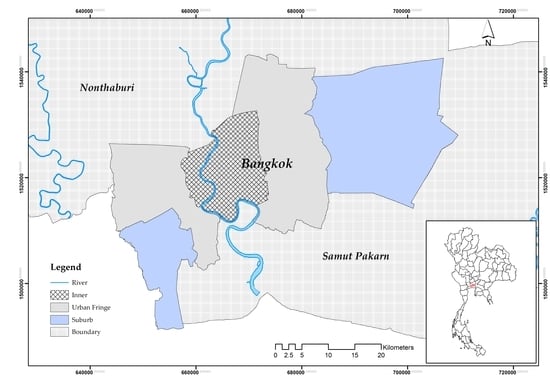
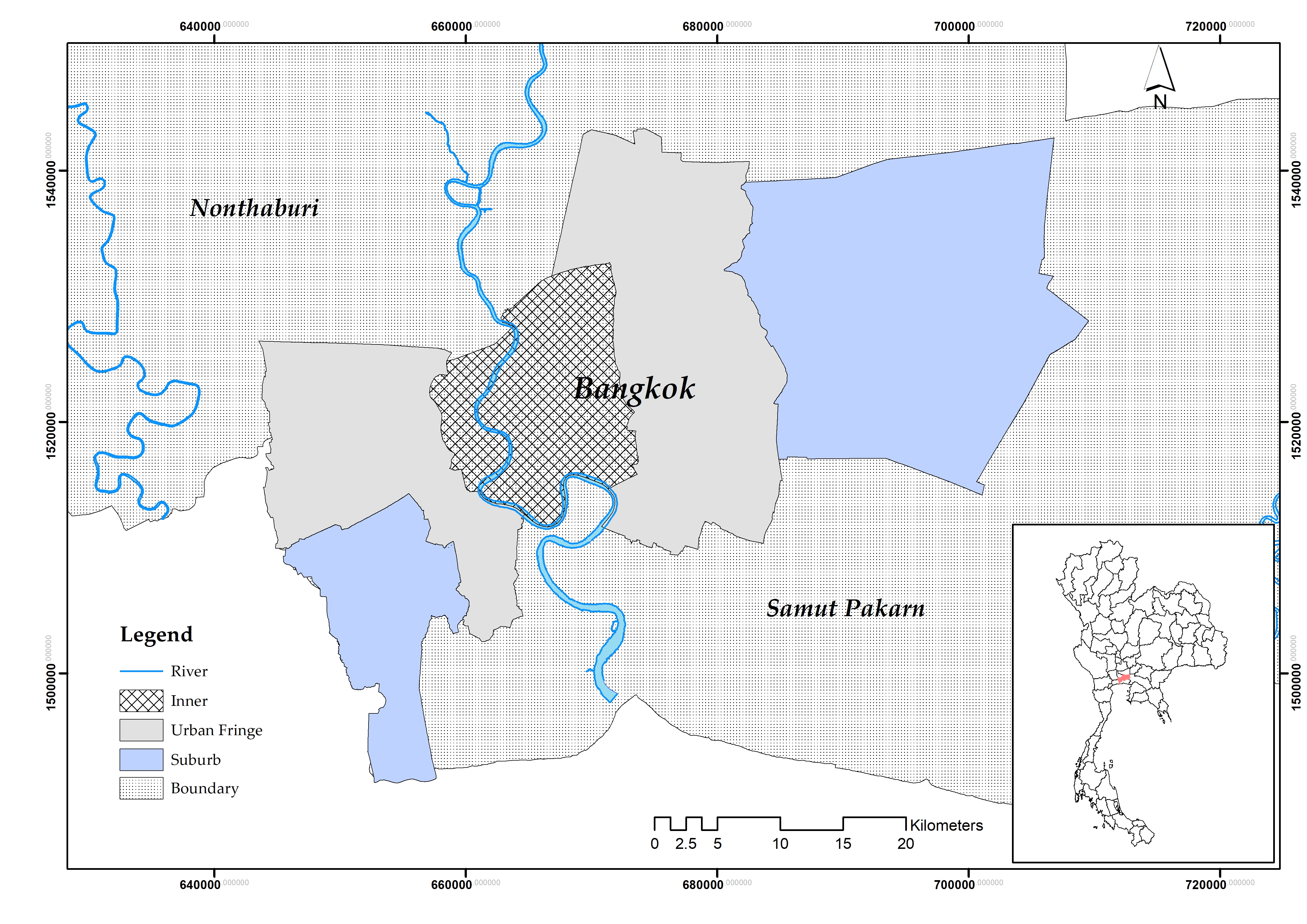
2.1. Study Area

The Bangkok Metropolitan Area (BMA) is the most economically developed city in Thailand (Figure 1) spread across 1568.7 km2, with 5,696,409, registered residents as of 2015 [36,37]. BMA is composed of 50 districts [38], which are divided into 3 main areas: inner city (22 districts, the old city center dominated by the historical conservation area, government offices, schools, and densely populated commercial areas), the urban fringe (22 districts, area of population expansion, commercial and residential activities, located within 10–20 km radius of the city center), and suburban areas (6 districts, the outer area of BMA, dominated by empty spaces and farming areas with a mixture of urban and rural) (Figure 1).

2.2. Medical Data

Monthly dengue data for 2009 and 2014 were obtained from the Bangkok Metropolitan Administration in the context of the DENFREE project [39] (Figure 2). The rates of incidence were calculated by dividing the number of dengue incidence by the total populations. Expected values were computed using the incidence rate (disease cases per 100,000 population) in each district from Equation (1) as follows:
IRdengue = (Cases/Population) × 100,000
where IRdengue is the incidence rate in each district; Cases are the total number of dengue incidence; and Population is the total population in each district.
The average annual dengue incidence rates during the study period were 135.0, 195.5, 186.4, 184.8, 264.6, and 98.0 per people in 2009–2014, respectively.

2.3. Methodology

2.3.1. Image Preprocessing

Landsat images provide space-based moderate-resolution remote sensing data. Landsat 5 Thematic Mapper (TM) and Landsat 8 Thermal Infrared sensor (TIRS) images were acquired from 2009 and 2014 and only clear-sky images were analyzed for the land surface temperature (LST) calculations in the three different zones (inner city, urban fringe, and suburban) (Figure 1). To avoid the impact of remote sensing data instability, the images in November were selected to explore the urban land surface temperature (LST).
A digital map of Bangkok, 1:4000 scale during 2009–2014, was obtained from the Town Planning Office Bangkok and used to categorize buildings into two groups as <8 floors (1–7 floors) and >8 floors (8–100 floors).
Time-series of LANDSAT 5 Thematic Mapper (TM) and LANDSAT 8 Thermal Infrared Sensor (TIRS) images (Path 129/Row 50, 51) acquired for 2009 and 2014 (LANDSAT 5 TM: 19 November 2009; LANDSAT 8 TIRS: 17 November 2014) were analyzed in this study. All of the images were clear and nearly cloud-free. Firstly, the radiometric and sun elevation correction was conducted. Next, the geometric correction was manipulated to be able to overlay and compare multi-temporal images or to interact with other mapping data. The LANDSAT images were rectified and georeferenced to the UTM map projection, datum WGS 84. Then, the images were resampled to 30 m using the nearest neighbor interpolation method to keep the brightness values of pixels unchanged. The root mean square (RMS) errors were less than 1 pixel.

2.3.2. Conversion of Digital Numbers to Radiance and LST

The LST calculation methods are based on LANDSAT 5 and LANDSAT 8 User’s Handbooks [40,41], which are widely used [37,42]. To retrieve LST, the steps are as follows.
First, the digital numbers (DN) of LANDSAT TM/TIRS thermal infrared bands were converted to radiance. For the LANDSAT 5 TM thermal infrared band (band 6: 10.40–12.50 µm), the following equation [40] was used:
Lλ = ((LMAX − LMIN)/(QCALMAX − QCALMIN)) × (QCAL − QCALMIN) + LMIN
where Lλ is the spectral radiance at the sensor’s aperture in W/(m2ster µm), LMAX and LMIN are the spectral radiance that is scaled to QCALMAX and QCALMIN in W/(m2ster µm), QCAL is the quantized calibrated pixel value in DN, and QCALMAX (= 255) and QCALMIN (=1) are the maximum and minimum quantized calibrated pixel values in DN.
For LANDSAT 8 TIRS thermal infrared bands (band 10: 10.60–11.19 and band 11: 11.50–12.51 µm), the radiance was calculated by using the following equation [41,43].
Lλ = ML × QCAL + AL
where Lλ is the top of atmosphere (TOA) spectral radiance in W/(m2srad µm), ML is the band-specific multiplicative rescaling factor from the metadata, AL is the band-specific additive rescaling factor from the metadata, and QCAL is the quantized and calibrated standard product pixel values.
Next, the radiance obtained from Equations (2) and (3) was converted to brightness temperature by using Equation (4) [40,41].
T = K2/ln [(K1/Lλ) + 1]
where T is the at-satellite brightness temperature in Kelvin (K), K2 is the calibration constant 2 = 1282.71 K (in case of LANDSAT 5 TM) or band-specific thermal conversion constant from the metadata (K2_CONSTANT_BAND_x, where x is the band number, 10 or 11) (in case of LANDSAT 8 TIRS), K1 is the Calibration constant 1 = 666.09 W/(m2sterµm) (in case of LANDSAT 5 TM) or band-specific thermal conversion constant from the metadata (K1_CONSTANT_BAND_x, where x is the band number, 10 or 11) (in case of LANDSAT 8 TIRS), Lλ is the spectral radiance at the sensor’s aperture in W/(m2ster µm) (in case of LANDSAT 5 TM) or top of atmosphere (TOA) spectral radiance in W/(m2srad µm).
Then, the brightness temperature was converted from Kelvin to °C using the following equation.
TS = T − 273.15
where TS is the surface radiance temperature in °C, T is at-satellite brightness temperature of a black body in Kevin. Finally, the surface radiance temperature maps of BMA at various times were calculated.
Land surface emissivity (LSE) is one of the key parameters to retrieve accurate LST from remotely sensed imagery. Landsat 5 (band 3, 4) and Landsat 8 (band 4, 5) were used to calculate the Normalized Difference Vegetation Index (NDVI). Then, the proportions of vegetation covering the BMA were calculated by using the equation [37,44] as shown:
Fr = (NDVI − NDVIbs)/(NDVI0 − NDVIbs)
where Fr is the fractional vegetation cover, NDVI is the Normalized Difference Vegetation Index, NDVIbs is the bare soil, and NDVI0 is the 100% vegetation cover NDVI.
To analyze the variation of surface temperature, the average surface temperature is calculated from the inner city, urban fringe, and suburb. Then, it is compared at each time period, such as monthly, seasonal, and yearly. The intensity of the urban heat island, UHII for the inner city, urban fringe, and suburb areas were determined by the following equations [37]:
UHII(inner-suburb) = surface temperature inner − surface temperature suburb
UHII(urban fringe-suburb) = surface temperature urban fringe − surface temperature suburb.
Then, the variation of surface temperatures and UHII in the inner city, urban fringe, and suburb areas were compared and described.

2.3.3. Statistical Analysis

Global Moran’s I statistic was used to identify characteristics of the global pattern to measure the correlation among spatial observations. Moran’s I was used to evaluate autocorrelation in dengue spatial distribution, testing how dengue incidence was clustered among districts [45,46,47].
Kernel density estimation is a method for examining large-scale trends in point pattern analysis, analyzing disease patterns and detecting hot spots. The approach estimates how event frequencies vary continuously across the study area based on the point patterns [46,48]. Figure 3 illustrates the kernel density approach in estimating event intensities from a number of points across a grid plate. In this example, the algorithm estimates the intensity by counting the number of building per km. Then, these intensity values were summed up to generate a final intensity value of each point. This method was applied by categorizing building density into low and high-rise building density in each zone (Figure 3). Figure 3 illustrates the distribution of buildings in the Bangkok Metropolitan Area in 2009 and 2014, respectively.
Generalized linear models were used to assess the association of vegetation coverage (Fr) with LST and built-up area with temperature.
Bayesian hierarchical modeling was used to model the spatial distribution of the relative incidence of dengue in Bangkok districts in years 2009 and 2014 to explore the association with the surface temperature and the number of buildings. For disease mapping of aggregate health data (district level in our case), a classical approach to relative risk analysis is the application of the model proposed by Besag, York, and Molliè (BYM model) [49]. For our analysis, we then assumed that the dengue incidence of 50 Bangkok districts {yi}, i = 1, …, 50, were conditionally independent observations with Poisson likelihood. That is, yi ~ Poisson (niθi) where ni is the population and θi is the relative incidence of district i. The logarithm function was adopted as the natural link function for Poisson modeling from Equation (9) to covariates of interest. Then, the relative incidence for each district was spatially modeled as
log(θi) = αi + β1 LB + β2 HB + β3 LBT + β4 HBT
where LBT and HBT are the surface temperature (°C) and LB and HB are the number of buildings per 1000 for each district i for low-story (LB) and high-story (HB) buildings with their corresponding coefficients, β1,…, β4. αi is the random intercept for each district, i.e., αi = β0 +ui +vi where β0 is the overall intercept. Under the BYM model, ui and vi are spatial and non-spatial random effects following the intrinsic conditional autoregressive and Gaussian models, respectively [49,50].
Since we used the Bayesian approach, prior distributions were specified for the parameters, β0,…, β4, ui and vi. For β0,…, β4, we assumed a non-informative Gaussian prior distribution with mean equal to zero and small precision (large variance) equal to 0.00005 [51]. The two precision hyper parameters for ui and vi, were specified according to a non-informative prior with Gamma (0.5, 0.0005) [51]. All the parameters were estimated using Bayesian inference, based on the Integrated Nested Laplace Approximations (INLA) [52] using the RStudio software version 1.1.463.

3. Results and Discussion

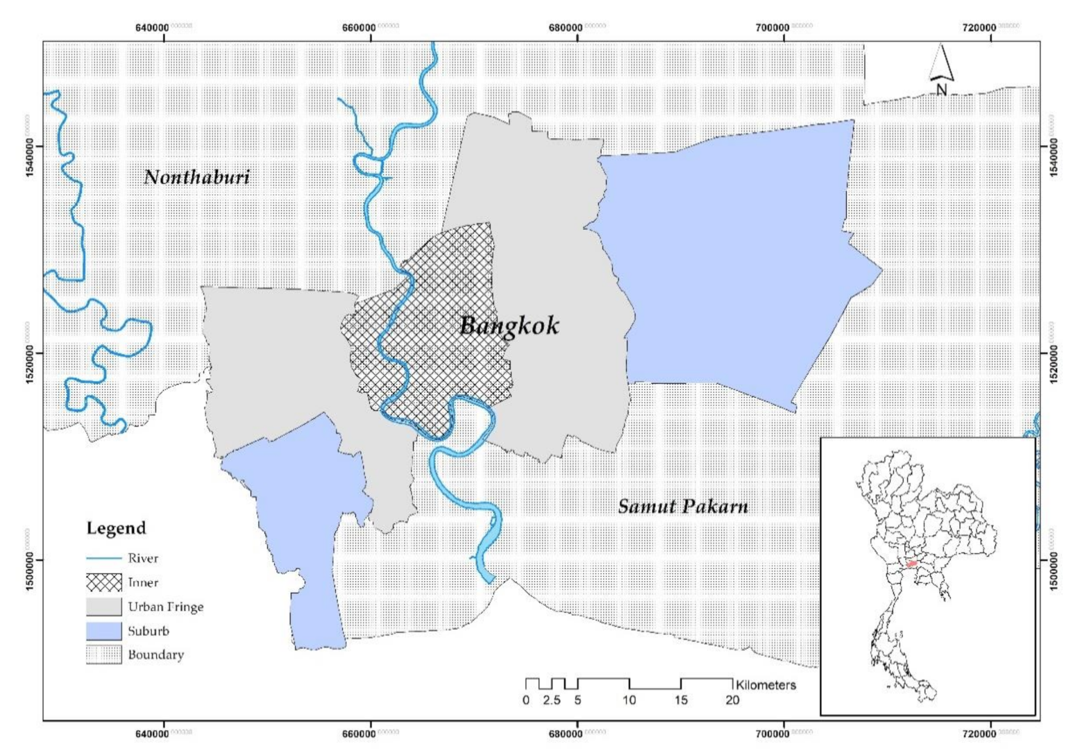
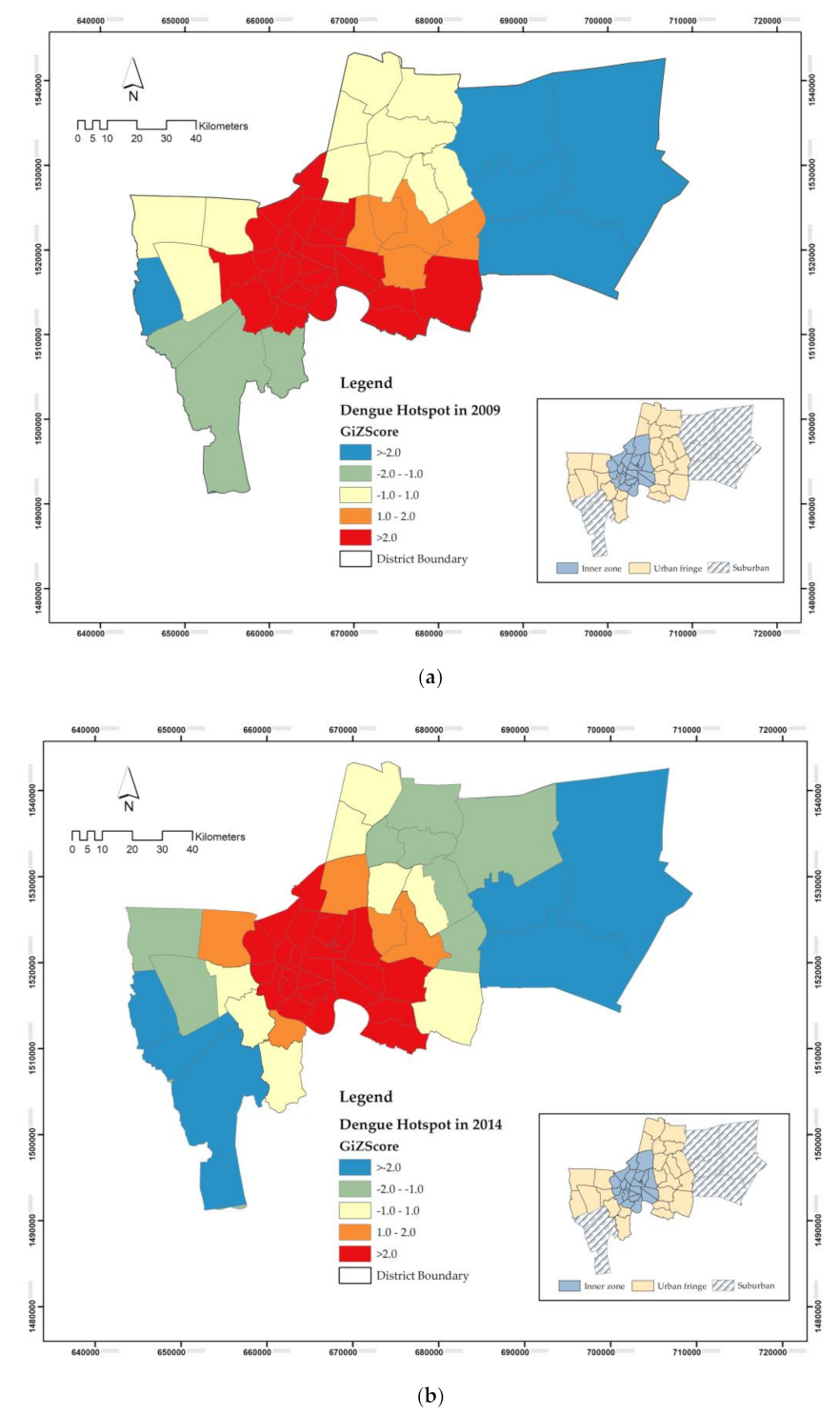
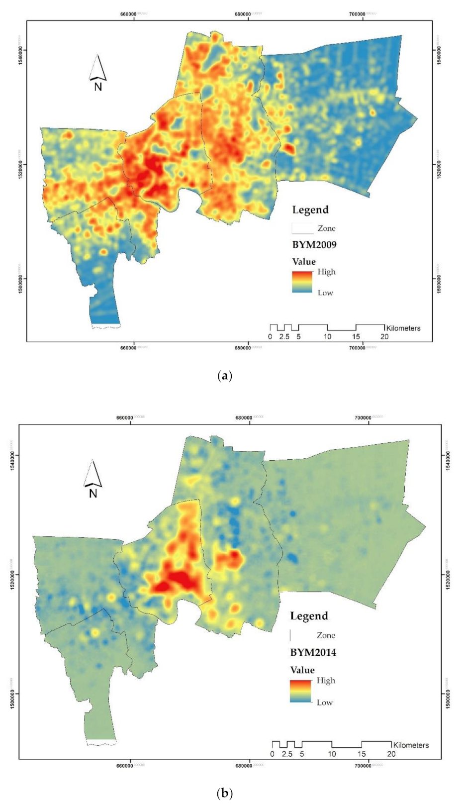
3.1. Dengue incidence map

Dengue incidence data were obtained from the Bangkok Metropolitan Administration. Figure 4a shows the location of significant local hotspots of spatial association using Moran’s I statistics. The Moran index reflects how neighboring values are associated with each other. Those locations were classified by type of association as the red and blue districts indicating spatial clusters (high surrounded by high (HH), and low surrounded by low (LL)), the orange and green indicating spatial outliers (high surrounded by low, and low surrounded by high). It was found that the cluster districts with high hotspots (HHHH) both in 2009 and 2014 were found in 15 districts (68%) in the inner zone and three districts (13%) in the urban fringe as shown in dark red, which are related to high-rise buildings distribution shown in Figure 3. The average incidence rates were 131 and 124 per 100,000 population in the inner zone and urban fringe in 2009 and 2014, respectively.

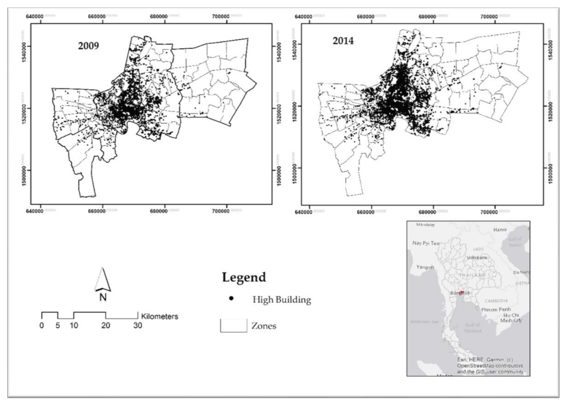
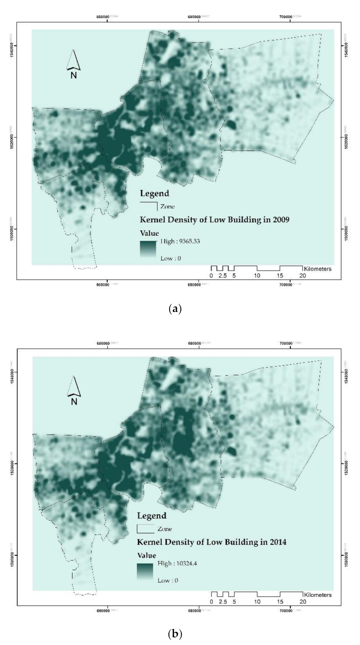
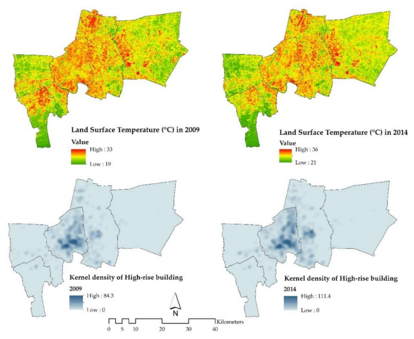
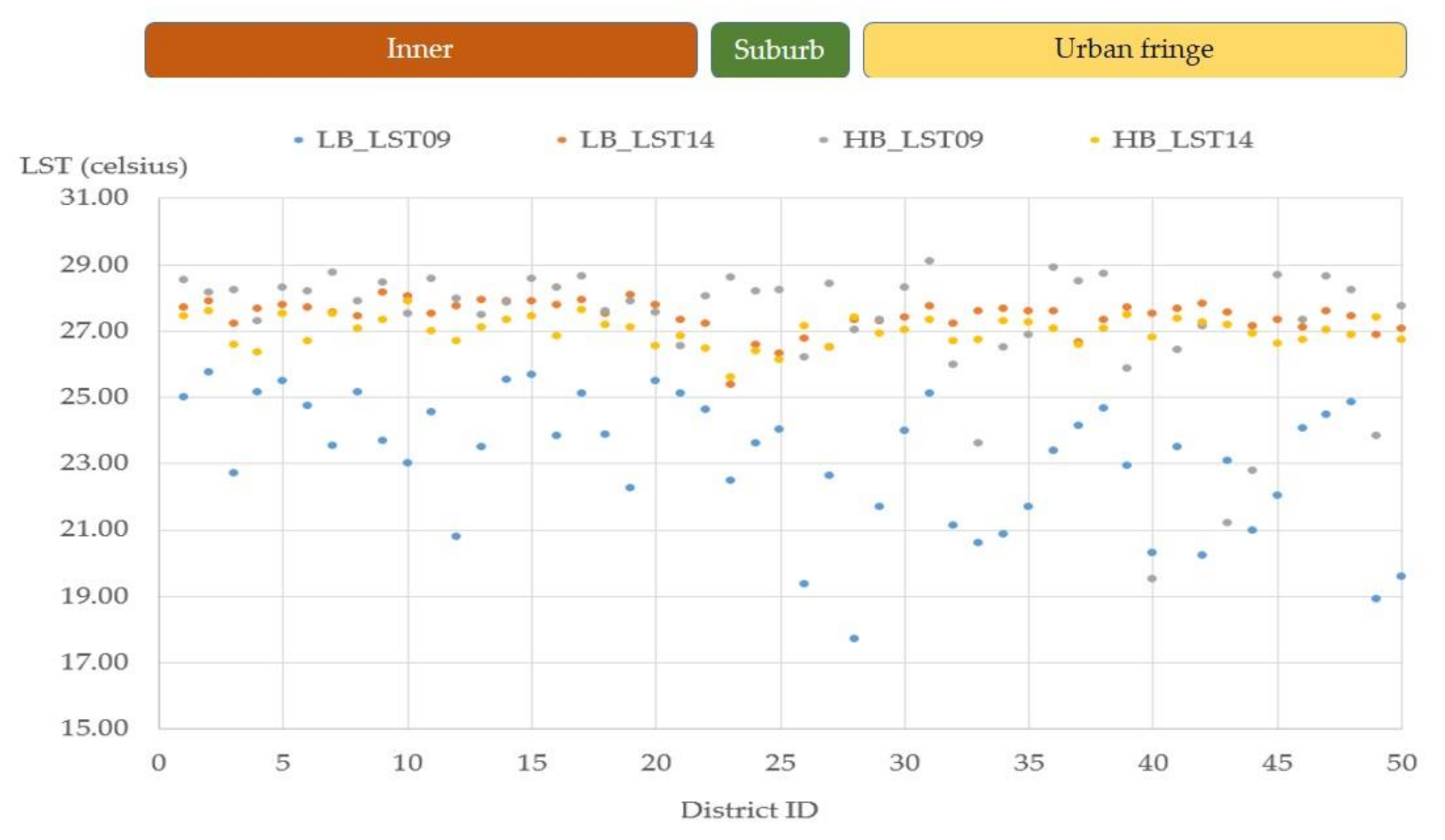
3.2. Distribution of Buildings with Land Surface Temperature

Figure 5 shows that the high-density level of increasing built-up area was distributed in the inner city and urban fringe. The areas with high LST expanded from the inner city to urban fringe; meanwhile, there were no substantial differences in LST in 2009 and 2014. The Landsat TM and TIRS thermal infrared bands worked very well at identifying the LST of BMA (Figure 6). The highest temperature occurred in November 2009 at 33 °C and in November 2014 at 36 °C. Figure 6 also compared the building density in 2009 and 2014. The highest building densities (per sq.km.) occurred in the inner city and expanded to the urban fringe, at 84.295 to 111.359, respectively.
The average LST within each urban zone was calculated by using the Landsat TM and TIRS Thermal Infrared band. These results showed that the increase of high-rise buildings from 2009 to 2014 was spatially different across these three zones. Meanwhile, these zones showed obvious average land surface temperature differences in low-rise buildings (<8 floors). The average land surface temperatures (°C) from 2009 to 2014 were 23.4 °C and 27.4 °C in the inner city, 22.8 °C and 27.4 °C in urban fringe, and 23.5 °C and 27.7 °C in the suburban zone, respectively, as shown in Table 1.
Meanwhile, considering the relationship between LST and vegetation coverage (Fr) from Equation (6), the vegetation coverage (Fr) negatively correlated with the surface temperature. In the dry season, R2 was 0.83 in 2009 and 0.79 in 2014 (Table 2).
Analysis of low-story building (LB) from three different zones was performed to observe the dynamic change of building density. The results found that the change in LB density was distributed in the increasing built-up area in the inner city, urban fringe, and suburbs, as shown in dark blue in Figure 5. The areas with the highest increase building density from 2009 to 2014 were found in the urban fringe both in the eastern and the western areas of Bangkok as shown in dark green in Figure 5a,b. From 2009 to 2014, there were 162,010 new buildings in BMA. Bangkok is experiencing rapid urban expansion. The buildings built in the inner city and urban fringe were large high-rise buildings and increased the amount of vertical high-density buildings. Figure 5 and Figure 6 and Table 1 shows the number of low-story buildings (LB) in BMA in 2009 and 2014. The growth rates of buildings in the inner city, urban fringe, and suburbs were 2.9, 5.0, and 3.6%, respectively, indicating that urban fringe changed rapidly compared to the other two zones. The LSTs in the inner city, urban fringe, and suburbs were 17.1, 20.2, and 17.9%, respectively, which is consistent with the building growth rate. The results showed that the surface temperature has increased by 4 °C in all urban zones over the 5-year period, and the spatial distribution of Surface UHIs was different between the three zones in 2009 and 2014. The result of this study related to the SUHI intensities in Bangkok of Keeratikasikron and Bonadoni (2018), who found that in the city core, high-density residential, commercial areas exhibit the highest mean SUHI intensities around 4 °C. Concerning the three zones, the warming effect of high density of buildings found in the inner city and the Don Mueang airport in the northern area of Bangkok with high temperature both in 2009 and 2014 [16].
Figure 7 shows that the correlation between temperature level and an increase in built-up density in different zones. R2 values were only 0.008, 0.0007, and 0.05 for inner city, urban fringe, and suburban areas, respectively. We found significant correlations between temperature levels and increased built-up area in both inner and suburban zones (p = 0.05 and 0.01, respectively). The increase in the number of high-rise buildings and higher building density affects LST and caused UHI phenomena in the city. The increased in high-rise buildings in inner and urban fringe areas is not a significant factor leading to the urban land surface temperature, because concrete was used for all of the construction in the whole inner city. The land surface temperatures are always high. Therefore, increased high-rise buildings in suburban areas would be a significant factor leading to urban LST. Hence, the urban heat island intensity (UHII) between the inner city and suburban areas of the BMA was higher than the UHII between the urban fringe and suburban areas. Concrete was used mostly for buildings and constructions in the urban fringe and suburban areas. It affected the reflection and absorbed energy from the sun. The increase in buildings and structures occurred and absorbed more energy from the sun than the ground and vegetation, making the surface temperature of the buildings higher. The result of the UHI phenomenon in the inner city is more heat than in the suburbs (Table 3). This corresponds to the cause of the UHI phenomenon [53]. The findings in this study also agree with Sanecharoen et al. (2019), where the increment of surface temperature because of existing concrete and asphalt materials was reported [37].

3.3. Surface Temperature Variation and the Intensity of Urban Heat Island in BMA

In 2009, the average LST in each zone in the inner city (23.9 °C) was higher than that in the urban fringe (21.3 °C) and suburban areas (20.8 °C). In 2014, the average LST in the inner city (28.1 °C) was likewise higher than the urban fringe (27.3 °C) and suburban areas (25.8 °C) (Table 3). In addition, the variation in urban land surface temperature in the urban fringe from 2009 and 2014 is the highest (6 °C), followed by the suburban area (5 °C) and inner city area (4 °C), respectively.
Meanwhile, for UHII from Equations (6) and (7), the UHII values between the inner city, urban fringe, and suburbs were determined as shown in Table 4. In 2009, there was a difference of 3.1 °C in the UHII between the inner city and suburban areas, while the UHII between the urban fringe and suburbs differed by 0.5 °C. In 2014, the UHII between the inner city and suburban areas was as high as 2.6 °C. The UHII between the urban fringe and suburban areas was as high as 1.7 °C. Thus, the UHII between the inner city and suburban areas was greater than with the UHII between the urban fringe and suburban areas.

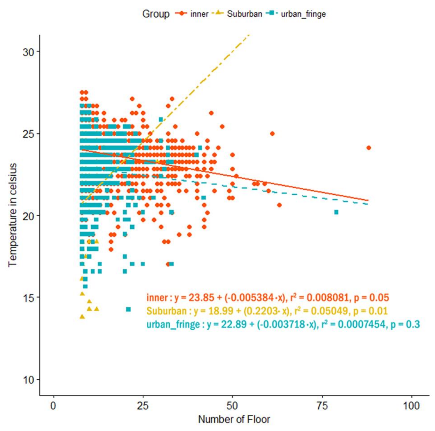
3.4. Relationship between LST and UHII with High-Rise Buildings in Different Three Zones

Bangkok is experiencing rapid urban expansion. The urban growth rate during 2000–2009 was 2.41% per year. The buildings located in the inner city and urban fringe were large high-rise buildings that increased the amount of vertical high-density buildings. The urban area in 2014 accounted for 56% of the BMA, as shown in Table 3. The buildings located in the inner city and urban fringe were large high-rise buildings and increased the quantity of vertical high-density buildings. The number of high-rise buildings of eight or more stories in the inner city and urban fringe areas of BMA from 2009 to 2014 increased. Due to limited city space, the buildings have increased vertically, especially in the inner city.
Figure 8 shows buildings in BMA in 2009 and 2014. The number of high-rise buildings of eight or more stories in the inner city and urban fringe areas of BMA from 2009 to 2014 increased by 49.4% and 79% respectively. In 2009 and 2014, there were 3071 and 4588 high-rise buildings (HB), respectively. The high-rise buildings in the inner city areas increased by 1494 units between 2009 and 2014, whereas in the urban fringe and suburb areas, they increased by 1076 and 45 units, respectively.
As can be seen in Figure 8, the LST of the low-rise buildings (LB: blue dots) in 2009 increased when the number of high-rise buildings (HB: gray dots) increased. It seems that the LST increases a lot in low-story buildings from 2009 to 2014. In addition, the LST in 2014 increased higher than the LST in 2009 in both the low-rise and high-rise buildings. The land surface temperature kept increasing with the high-rise building density. Both the low-rise buildings (LB: red dots) and high-rise buildings (HB: yellow dots) had high land surface temperatures, although the LST changed within different zones, as shown in Figure 8. The area percentages of the low-rise buildings in 2014 was larger than the LST in 2009 both in urban fringe and suburban areas, whereas the proportion of area inner zones had the same probability of LST. These results confirm that the roles played by the difference in energy consumption between inner city, suburban, and urban fringe areas are mainly because the cooling load of urban buildings is 13% higher than that of similar buildings in the rural–urban fringe areas. Thus, this relationship between electricity consumption and temperature has been clearly established [20,54,55,56].

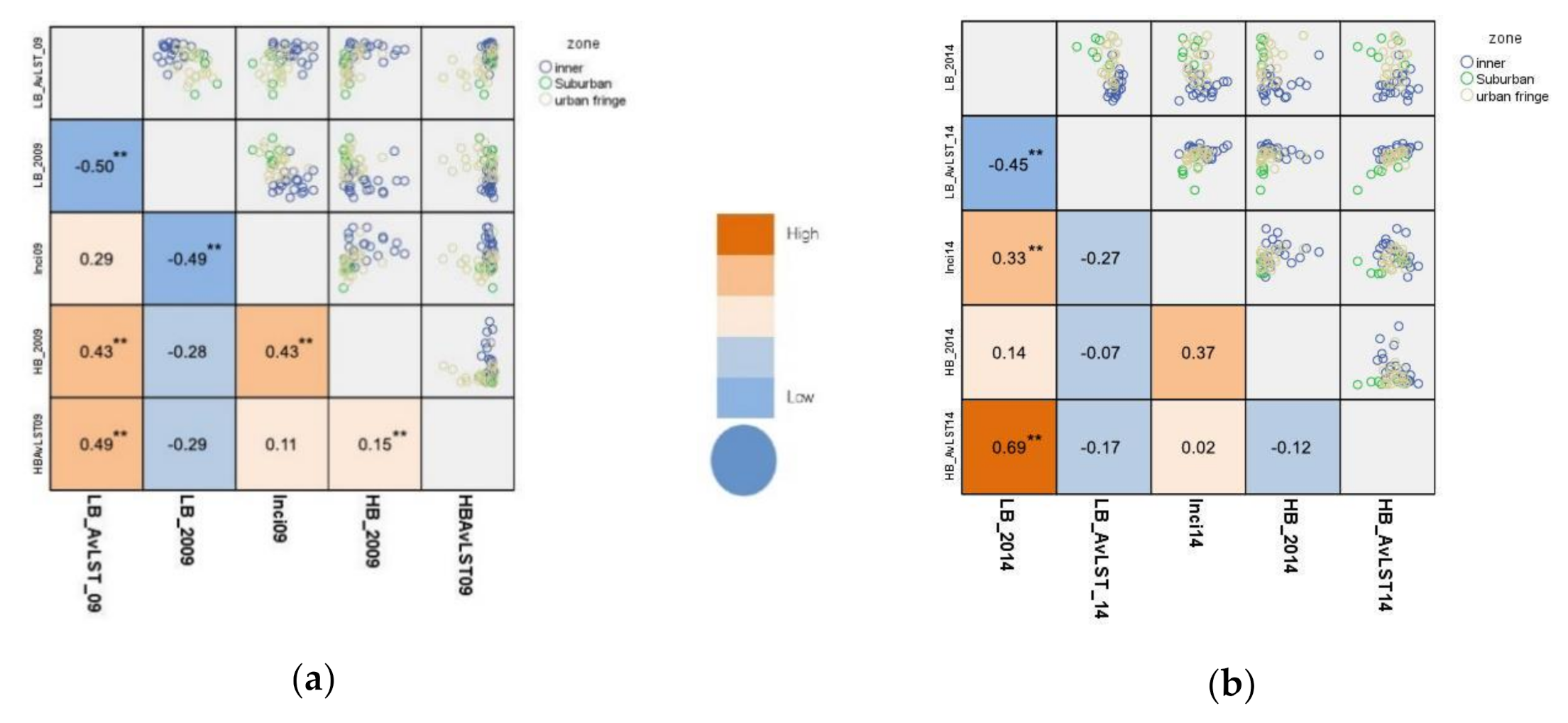
3.5. Correlation Coefficients between LST, Number of Buildings, and Dengue Incidence Per District

The Pearson correlation coefficients between dengue incidence per district, building density, and land surface temperature were calculated to analyze the relationship between dengue incidence and land surface temperature at the time of occurrence. The highest correlation of average LST was seen in 2009 at the same time of occurrence. The coefficient for 2014 showed the highest correlation with the density of high-rise buildings (HB).
To relate the LST to dengue incidences, the correlation between the building density and LST level for the low-rise and high-rise building was analyzed. The highest positive correlations were found between the number of high-rise buildings (HB) and dengue incidences both in 2009 and 2014 as 0.43 ** and 0.37, respectively. Correlation is significant at the p-value < 0.01 (2-tailed). The relationship between land surface temperatures and dengue incidences is shown in Figure 9a 2009 and Figure 9b 2014 with 85 and 75% of high dengue cases surrounded by high dengue cases (HH) in the inner city by Moran’s I statistical analysis, respectively. Meanwhile, the relationship between LST and dengue incidences by HH in 2009 and 2014 in the urban fringe are 15 and 26%, respectively. Pearson correlation was used to calculate the correlation matrix (Figure 9 and Appendix A). In each zone, the LST data were extracted from the satellite imageries for each year using statistical analysis. The highest positive correlations in 2009 were the density of high-rise buildings in each zone with dengue incidence at 0.43 **. High negative correlations were found between the average LST in all of the zones of the low-rise buildings at −0.49 *. The highest positive correlation in 2014 was the density of high-rise buildings and dengue incidences at 0.37. A high correlation was also found between the average LST each zone and dengue incidences at 0.33 **, which had a significant influence on urban land surface temperature. As shown in Figure 9 and Table A1, changes in the building density in each zone are highly correlated to changes in LST and dengue incidences, which had a significant influence on land surface temperature. In 2009, the highest correlations between LST and dengue incidence in 2009 were found in the inner and suburb areas. In 2014, the highest correlations were found in all zones of HB LST and LB density at 0.69 **. This means that the increasing of low-rise buildings density had a significant influence on land surface temperature. In addition, the density of low-rise buildings also generates high surface temperature. This means the dengue incidence occurred in the inner and suburban areas in 2009 and was expanded to both the HB and LB areas in 2014.
Table 4 shows the mean, median, standard deviation (SD), and 95% credible interval (CrI) of the association (each coefficient, β) between dengue incidence and socio-environmental covariates for Bangkok districts in 2009 and 2014. The comparison of mean incidence rates implies the number of high-rise buildings and both the number of high-rise buildings and surface temperature of low-rise buildings increased dengue incidence in years 2009 and 2014, respectively. However, the number of high-rise buildings was only significant (CrI of incidence does not include 1) with mean relative incidence = exp(0.7857) = 2.19 (95%CrI: 1.16, 4.16) in 2009. This means for every 1000 new high-rise buildings, the dengue incidence could increase 2.19 on average during that time period. Figure 10 shows the results of the spatial distribution of the relative incidence of dengue in Bangkok districts in years 2009 and 2014 to explore the association with the surface temperature and the number of buildings by the Bayesian hierarchical modeling (BYM) approach.

4. Conclusions

To relate the LST to dengue incidences, the correlation between the building density and LST level for buildings less than eight floors (LB) and buildings with 8 or more floors (HB) was analyzed. The highest positive correlations were found between the number of high-rise building (≥8 floors) and dengue incidences both in 2009 and 2014. In addition, positive correlations were found between the number of LB and the average LST with dengue incidences both in 2009 and 2014. The highest negative correlations were found between dengue incidences and the average LST of LB.
The areas with higher building density in the inner city and urban fringe zones are at higher risk of being dengue hotspots, as shown in the dark red areas in Figure 4. The building density and high-rise building distribution in the vertical city were used to estimate the density and identify the areas where the risk of a diseases outbreak is higher (Figure 6 and Figure 7). The areas with high LST expanded from the inner city zone to the urban fringe (Figure 6). We found significant correlations between temperature levels and increases of built-up area and building density in suburban zones. Meanwhile, an increase of built-up area in the inner city and urban fringe found non-significant correlation with LST. LST was always at a high temperature level.
This paper has explored the potential of geo-information technology to analyze the spatial factors affecting dengue fever and land surface temperature. Geospatial technology is important for the understanding of spatial correlation between epidemiological studies and urban land surface temperature by satellite images. The results of this study lead to further understanding changes in spatial patterns of urbanization from the past to the present or to investigate how spatial patterns will change from the present to the future in terms of vertical city. Temperature was an important variable related to the prediction of dengue incidence in the tropical zone [47,56,57,58,59,60]. The study of Sarfraz et al. (2014), performed in Thailand, found that a temperature range between 30–35 °C had a high impact on Aedes vector breeding. Nakhapakorn and Tripathi (2005) and Ssempiira et al. (2017) found that temperature indices of dengue with a lag of time 2–4 weeks were related to the dengue incidence rate [47,61].
In the Bangkok Metropolitan Area, dengue incidence has been associated with LST. LST was one of the variables that was significantly associated with vertical city development, urban expansion, and human dengue incidence. In this study, high dengue incidence was related to the building density and LST level for buildings with eight floors or more.
The Pearson correlation coefficients between incidence, building density, and land surface temperature were calculated to analyze the relationship between dengue cases and land surface temperature at the same time of occurrence. The highest correlation of average LST was seen in 2009 at the same time of occurrence. For 2014, dengue incidence had the highest correlation with the density of high-rise buildings (≥ eight floors). Positive correlations were also found between dengue incidence and average LST. These findings could be used for urban planning such as the surveillance system by BMA and environmental monitoring of the significant relationship aspects obtained from this study.
In the future, new IT technologies, including data sciences, object recognition, and time-series analysis, can derive data to estimate infectious disease trends enabling more accurate predictions for vector-borne diseases. Further studies in epidemic forecasting are still needed to exploit the power of big data, machine learning, artificial intelligence, and geospatial technology to identify the association of high-risk factors influencing the epidemic outbreak. The Sustainable Development Goals set out by the 2030 Agenda for Sustainable Development propose goals, which involve creating green public spaces and improving urban planning and management to make cities sustainable, safe, and resilient. Developing adaptation strategies for UHI and climate change to improve the resilience of the city has been considered as the future direction of the city planning. There are also limitations existing in this study for the lack of non-anthropogenic parameters, climate scenarios, and geo-information technology such as digital surface model (DSM) and digital terrain from Light Detection and Ranging (LIDAR) data and very high-resolution satellite imageries need to be improved for the prediction. Future work on these parameters for finding links between UHI and dengue incidences is recommended. Therefore, it is of great scientific significance to study the impact of urban expansion on the UHI effect to improve the adaptability and resilience of cities to climate change for the Bangkok Metropolitan Administration and Ministry of Public Health. This study has several limitations. Firstly, the spatial scale of the dengue incidence data is at a relatively coarse scale (district) and much more so than the spatial scale that is possible for estimates of built-up area and LST. However, insofar as dengue occurs in spatial clusters, very fine geographical scale analyses would be confronted with a non-independence of locally occurring dengue cases. Secondly, the division of Bangkok into three zones is somewhat arbitrary, but it at least enables a broad differentiation of Bangkok into the recognizably different suburban and central city areas with a buffer area in between.

Author Contributions

Conceptualization, K.N., K.T., A.M., S.J., and R.O.; methodology, K.N.; software, K.N., C.R., K.T., and W.S.; validation, K.N., A.M., R.P., and R.O.; formal analysis, K.N.; investigation, K.N.; resources, K.N.; data curation, K.N., C.R., and K.T.; writing—original draft preparation, K.N.; writing—review and editing, K.N., K.T., R.P.; visualization, K.N.; supervision, A.M., and R.O.; project administration, K.N., and R.P.; funding acquisition, R.P., and K.N. All authors have read and agreed to the published version of the manuscript.

Funding

This research was partial funded by “Dengue Framework for Resisting Epidemics in Europe studies (DENFREE)” were funded by the European Union 7th FP, grant number 282378.

Acknowledgments

The authors would like to thank the Bangkok Metropolitan Administration and DENFREE project for their support. In addition, thank you to the staffs of Faculty of Environment and Resource Studies, Mahidol University and other agencies that support the information in the research.

Conflicts of Interest

The authors declare no conflict of interest.

Appendix A

Table A1. Pearson correlation between numbers of building, average land surface temperature (LST), and dengue incidence in 2009 and 2014.
No. of Building < 8Fl.Average LST (°C) < 8Fl.Dengue IncidenceNo. of Building > 8Fl.Average LST (°C) > 8Fl.
No. of Building
<8Fl.
Pearson Correlation1−0.504 **−0.496 **−0.282−0.289 **
2009Sig. (2-tailed) 000.0470.042
Average LST (°C) 2009Pearson Correlation−0.504 **10.299 *0.434 **0.489
No. of Building
<8Fl.
Sig. (2-tailed)0 0.0350.0020
Dengue Incidence Pearson Correlation−0.496 **0.299*10.425 **0.112 *
2009Sig. (2-tailed)00.035 0.0020.439
No. of Building
>8Fl.
Pearson Correlation−0.282 *0.434**0.425 **1 *0.147 **
2009Sig. (2-tailed)0.0470.0020.002 0.309
Average LST (°C)Pearson Correlation−0.289 *0.489 **0.1120.147 *1 **
No. of Building
>8Fl.
Sig. (2-tailed)0.04200.4390.309
2009
No. of Building
<8Fl.
Pearson Correlation1−0.455 **−0.269−0.074−0.171 **
2014Sig. (2-tailed) 0.0010.0590.6090.235
Average LST (°C)Pearson Correlation−0.455 **10.333 *0.141 **0.694
No. of Building
<8Fl.
Sig. (2-tailed)0.001 0.0180.3270
2014
Dengue Incidence Pearson Correlation−0.2690.333 *10.3670.024 *
2014Sig. (2-tailed)0.0590.018 0.0090.866
No. of Building
>8Fl.
Pearson Correlation−0.0740.1410.367 **10.121
2014Sig. (2-tailed)0.6090.3270.009 0.401
Average LST (°C)Pearson Correlation−0.1710.694 **0.024−0.1211 **
No. of Building
>8Fl.
Sig. (2-tailed)0.23500.8660.401
2014
*. Correlation is significant at the 0.05 level (2-tailed). **. Correlation is significant at the 0.01 level (2-tailed).

References

  1. World Health Organization. Global Vector Control Response 2017–2030; License: CC BY-NC-SA 3.0 IGO; World Health Organization: Geneva, Switzerland, 2017; ISBN 978-92-4-151297-8. [Google Scholar]
  2. World Health Organization. Dengue and Dengue Hemorrhagic Fever; Fact Sheet 117, Revised February 2015; World Health Organization: Geneva, Switzerland, 2015; Available online: http://www.who.int/mediacentre/factsheets/fs117/en/ (accessed on 22 January 2020).
  3. Guzman, M.G.; Halstead, S.B.; Artsob, H.; Buchy, P.; Farrar, J.; Gubler, D.J.; Hunsperger, E.; Kroeger, A.; Margolis, H.S.; Martínez, E.; et al. Dengue: A continuing global threat. Nat. Rev. Microbiol. 2010, 8 (Suppl. S12), S7–S16. [Google Scholar] [CrossRef] [PubMed] [Green Version]
  4. Daudé, E.; Mazumdar, S.; Solanki, V. Widespread Fear of Dengue Transmission but Poor Practices of Dengue Prevention: A Study in the Slums of Delhi, India. PLoS ONE 2017, 12, e0171543. [Google Scholar] [CrossRef] [Green Version]
  5. Bhatt, S.; Gething, P.W.; Brady, O.J.; Messina, J.P.; Farlow, A.W.; Moyes, C.L.; Drake, J.M.; Brownstein, J.S.; Hoen, A.G.; Sankoh, O.; et al. The global distribution and burden of dengue. Nature 2013, 496, 504–507. [Google Scholar] [CrossRef] [PubMed]
  6. Gubler, D.J. Epidemic dengue/dengue hemorrhagic fever as a public health, social and economic problem in the 21st century. Trends Microbiol. 2002, 10, 100–103. [Google Scholar] [CrossRef]
  7. Kyle, J.L.; Harris, E. Global Spread and Persistence of Dengue. Annu. Rev. Microbiol. 2008, 62, 71–92. [Google Scholar] [CrossRef] [Green Version]
  8. Hii, Y.L.; Zhu, H.; Ng, N.; Ng, L.C.; Rocklöv, J. Forecast of Dengue Incidence Using Temperature and Rainfall. PLoS Negl. Trop. Dis. 2012, 6, e1908. [Google Scholar] [CrossRef] [Green Version]
  9. Paul, R.; Sousa, C.A.; Sakuntabhai, A.; Devine, G. Mosquito control might not bolster imperfect dengue vaccines. Lancet 2014, 384, 1747–1748. [Google Scholar] [CrossRef] [PubMed]
  10. Liu-Helmersson, J.; Stenlund, H.; Wilder-Smith, A.; Rocklöv, J. Vectorial capacity of Aedes aegypti: Effects of temperature and implications for global dengue epidemic potential. PLoS ONE 2014, 9, e89783. [Google Scholar] [CrossRef] [Green Version]
  11. Lowe, R.; Cazelles, B.; Paul, R.; Rodó, X. Quantifying the added value of climate information in a spatio-temporal dengue model. Stoch. Environ. Res. Risk Assess. 2016, 30, 2067–2078. [Google Scholar] [CrossRef]
  12. Misslin, R.; Telle, O.; Daudé, É.; Vaguet, A.; Paul, R.E. Urban climate versus global climate change-what makes the difference for dengue? Ann. N. Y. Acad. Sci. 2016, 1382, 56–72. [Google Scholar] [CrossRef]
  13. Misslin, R.; Daudé, É. An environmental suitability index based on the ecological constraints of Aedes aegypti, vector of dengue and Zika virus. RIG Int. Rev. Geomat. 2017, 27, 481–501. [Google Scholar] [CrossRef]
  14. Telle, O.; Vaguet, A.; Yadav, N.K.; Lefebvre, B.; Cebeillac, A.; Nagpal, B.N.; Daudé, E.; Paul, R.E. The Spread of Dengue in an Endemic Urban Milieu—The Case of Delhi, India. PLoS ONE 2016, 11, e0146539. [Google Scholar] [CrossRef] [PubMed] [Green Version]
  15. United Nations, Department of Economic and Social Affairs, Population Division. World Urbanization Prospects: The 2018 Revision (ST/ESA/SER.A/420); United Nations: New York, NY, USA, 2019. [Google Scholar]
  16. Keeratikasikron, C.; Bonadoni, S. Urban heat island analysis over the land use zoning plan of Bangkok by means of Landsat 8 imagery. Remote Sens. 2018, 10, 440. [Google Scholar] [CrossRef]
  17. Montaner-Fernandez, D.; Morales-Salinas, L.; Rodriguez, J.S.; Cárdenas-Jirón, L.; Huete, A.; Fuentes-Jaque, G.; Pérez-Martínez, W.; Cabezas, J. Spatio-Temporal variation of the urban heat island in Santiago, Chile during summers 2005–2017. Remote Sens. 2020, 12, 3345. [Google Scholar] [CrossRef]
  18. Meng, C.; Dou, Y. Quantifying the anthropogenic footprint in Eastern China. Sci. Rep. 2016, 6, 24337. [Google Scholar] [CrossRef] [PubMed] [Green Version]
  19. Alonso, L.; Renard, F. A new approach for understanding urban microclimate by integrating complementary predictors at different scales in regression and machine learning models. Remote Sens. 2020, 12, 2434. [Google Scholar] [CrossRef]
  20. Yang, J.; Santamouris, M. Urban heat island and mitigation technologies in Asian and Australian Cities—Impact and mitigation. Urban Sci. 2018, 2, 74. [Google Scholar] [CrossRef] [Green Version]
  21. Sun, Y.; Gao, C.; Li, J.; Wang, R.; Liu, J. Quantifying the effects of urban form on land surface temperature in subtropical high-density urban areas using machine learning. Remote Sens. 2019, 11, 959. [Google Scholar] [CrossRef] [Green Version]
  22. Jed Collins, J.; Dronova, I. Urban landscape change analysis using local climate zones and object-based classification in the Salt lake metro region, Utah, USA. Remote Sens. 2019, 11, 1615. [Google Scholar] [CrossRef] [Green Version]
  23. Chen, M.; Zhou, Y.; Hu, M.; Zhou, Y. Influence of urban scale and urban expansion on the urban heat island effect in metropolitan areas: Case study of Beijing-Tianjin-Hebei urban agglomeration. Remote Sens. 2020, 12, 3491. [Google Scholar] [CrossRef]
  24. Seto, K.C.; Fragkias, M.; Guneralp, B.; Reilly, M.K. A meta-analysis of global urban land expansion. PLoS ONE 2011, 6, e23777. [Google Scholar] [CrossRef] [PubMed]
  25. Li, J.; Song, C.; Cao, L.; Zhu, F.; Meng, X.; Wu, J. Impacts of landscape structure on surface urban heat islands: A case study of Shanghai, China. Remote Sens. Environ. 2011, 115, 3249–3263. [Google Scholar] [CrossRef]
  26. Peng, J.; Xie, P.; Liu, Y.; Ma, J. Urban thermal environment dynamics and associated landscape pattern factors: A case study in the Beijing metropolitan region. Remote Sens. Environ. 2016, 173, 145–155. [Google Scholar] [CrossRef]
  27. Feng, Y.; Gao, C.; Tong, X.; Chen, S.; Lei, Z.; Wang, J. Spatial Patterns of Land Surface Temperature and Their Influencing Factors: A Case Study in Suzhou, China. Remote Sens. 2019, 11, 182. [Google Scholar] [CrossRef] [Green Version]
  28. Fu, P.; Weng, Q. A time series analysis of urbanization induced land use and land cover change and its impact on land surface temperature with Landsat imagery. Remote Sens. Environ. 2016, 175, 205–214. [Google Scholar] [CrossRef]
  29. Liu, K.; Fang, J.-Y.; Zhao, D.; Liu, X.; Zhang, X.-H.; Wang, X.; Li, X.-K. An Assessment of Urban Surface Energy Fluxes Using a Sub-Pixel Remote Sensing Analysis: A Case Study in Suzhou, China. ISPRS Int. J. Geo-Inf. 2016, 5, 11. [Google Scholar] [CrossRef]
  30. Rotem-Mindali, O.; Michael, Y.; Helman, D.; Lensky, I.M. The role of local land-use on the urban heat island effect of Tel Aviv as assessed from satellite remote sensing. Appl. Geogr. 2015, 56, 145–153. [Google Scholar] [CrossRef]
  31. Jenerette, G.D.; Harlan, S.L.; Buyantuev, A.; Stefanov, W.L.; Declet-Barreto, J.; Ruddell, B.L.; Myint, S.W.; Kaplan, S.; Li, X.X. Micro-scale urban surface temperatures are related to land-cover features and residential heat related health impacts in Phoenix, AZ USA. Landsc. Ecol. 2016, 31, 745–760. [Google Scholar] [CrossRef]
  32. Deilami, K.; Kamruzzaman, M.; Liu, Y. Urban heat island effect: A systematic review of spatio-temporal factors, data, methods, and mitigation measures. Int. J. Appl. Earth Obs. Geoinf. 2018, 67, 30–42. [Google Scholar] [CrossRef]
  33. Rivera, E.; Antonio-Némiga, X.; Origel-Gutiérrez, G.; Sarricolea, P.; Adame-Martínez, S. Spatiotemporal analysis of the atmospheric and surface urban heat islands of the Metropolitan Area of Toluca, Mexico. Environ. Earth Sci. 2017, 76, 137. [Google Scholar] [CrossRef]
  34. Heaviside, C.; Macintyre, H.; Vardoulakis, S. The Urban Heat Island: Implications for Health in a Changing Environment. Curr. Envir. Health Rep. 2017, 4, 296–305. [Google Scholar] [CrossRef] [PubMed]
  35. Su, Y.-F.; Foody, G.M.; Cheng, K.-C. Spatial non-stationarity in the relationships between land cover and surface temperature in an urban heat island and its impacts on thermally sensitive populations. Landsc. Urban Plan. 2012, 107, 172–180. [Google Scholar] [CrossRef]
  36. Bangkok Information Center. Bangkok Nowadays. Available online: http://www.bangkokgis.com/gis_information/population/ (accessed on 20 January 2019). (In Thai).
  37. Sanecharoen, W.; Nakhapakorn, K.; Mutchimwong, A.; Jirakajohnkool, S.; Onchang, R. Assessment of Urban Heat Island Patterns in Bangkok Metropolitan Area Using Time-Series of LANDSAT Thermal Infrared Data. Environ. Nat. Resour. J. 2019, 17, 87–102. [Google Scholar] [CrossRef]
  38. Department of City Planning. Final Report of the Project on BMA Central City Planning; Department of City Planning BMA: Bangkok, Thailand, 2011. (In Thai) [Google Scholar]
  39. Jaenisch, T.; Sakuntabhai, A.; Wilder-Smith, A.; DengueTools. Dengue research funded by the European Commission-scientific strategies of three European dengue research consortia. PLoS Negl. Trop. Dis. 2013, 7, e2320. [Google Scholar] [CrossRef] [PubMed]
  40. NASA (National Aeronautics and Space Administration). Landsat 7 Science Data User’s Handbook. 2011. Available online: https://www.usgs.gov/media/files/landsat-7-data-users-handbook (accessed on 18 October 2014).
  41. US Geological Survey. Landsat 8 Data Users Handbook. 2019. Available online: https://www.usgs.gov/media/files/landsat-8-data-users-handbook (accessed on 30 May 2019).
  42. Weng, Q. Thermal infrared remote sensing for urban climate and environmental studies: Methods, applications, and trends. ISPRS J. Photogram. 2009, 64, 335–344. [Google Scholar] [CrossRef]
  43. Isaya Ndossi, M.; Avdan, U. Application of Open Source Coding Technologies in the Production of Land Surface Temperature (LST) Maps from Landsat: A PyQGIS Plugin. Remote Sens. 2016, 8, 413. [Google Scholar] [CrossRef] [Green Version]
  44. Song, W.; Gaiyan Ruan, X.M.; Gao, Z.; Li, L.; Yan, G. Estimating fractional vegetation cover and the vegetation index of bare soil and highly dense vegetation with a physically based method. Int. J. Appl. Earth Obs. 2017, 58, 168–176. [Google Scholar] [CrossRef]
  45. Nakhapakorn, K.; Jirakajohnkool, S. Temporal and Spatial Autocorrelation Statistics of Dengue Fever. Dengue Bull. 2006, 30, 177–183. [Google Scholar]
  46. Jeefoo, P.; Tripathi, N.K.; Souris, M. Spatio-temporal diffusion pattern and hotspot detection of dengue in Chachoengsao province, Thailand. Int. J. Environ. Res. Public Health 2011, 8, 51–74. [Google Scholar] [CrossRef] [Green Version]
  47. Nakhapakorn, K.; Tripathi, N.K. An information value based analysis of physical and climatic factors affecting dengue fever and dengue haemorrhagic fever incidence. Int. J. Health Geogr. 2005, 4, 13. [Google Scholar] [CrossRef] [Green Version]
  48. Lai, P.C.; Low, C.T.; Wong, M.; Wong, W.C.; Chan, M.H. Spatial analysis of falls in an urban community of Hong Kong. Int. J. Health Geogr. 2009, 8, 14. [Google Scholar] [CrossRef]
  49. Besag, J.; York, J.; Mollié, A. Bayesian image restoration, with two applications in spatial statistics. Ann. Inst. Statist. Math. 1991, 43, 1–20. [Google Scholar] [CrossRef]
  50. Lawson, A.B.; Banerjee, S.; Haining, R.P.; Ugarte, M.D. Handbook of Spatial Epidemiology; CRC Press: Boca Raton, FL, USA, 2016; ISBN 9781482253016. [Google Scholar]
  51. Costa, J.V.; Donalisio, M.R.; Silveira, L.V.d.A. Spatial distribution of dengue incidence and socio-environmental conditions in Campinas, São Paulo State, Brazil, 2007. Cadernos de Saude Publica 2013, 29, 1522–1532. [Google Scholar] [CrossRef] [PubMed]
  52. Rue, H.; Martino, S.; Chopin, N. Approximate Bayesian inference for latent Gaussian models by using integrated nested Laplace approximations. J. R. Stat. Soc. Ser. B 2009, 71, 319–392. [Google Scholar] [CrossRef]
  53. US Environmental Protection Agency. Reducing Urban Heat Islands: Compendium of Strategies—Chapter 1: Urban Heat Island Basics. 2014. Available online: http://www.epa.gov/heatisld/resources/pdf/BasicsCompendium.pdf (accessed on 15 October 2014).
  54. Santamouris, M. On the energy impact of urban heat island and global warming on buildings. Energy Build. 2014, 82, 100–113. [Google Scholar] [CrossRef]
  55. Chen, M.; Ban-Weiss, G.A.; Sanders, K.T. The role of household level electricity data in improving estimates of the impacts of climate on building electricity use. Energy Build. 2018, 180, 146–158. [Google Scholar] [CrossRef]
  56. Parselia, E.; Kontoes, C.; Tsouni, A.; Hadjichristodoulou, C.; Kioutsioukis, I.; Magiorkinis, G.; Stilianakis, N.I. Satellite Earth Observation Data in Epidemiological Modeling of Malaria, Dengue and West Nile Virus: A Scoping Review. Remote Sens. 2019, 11, 1862. [Google Scholar] [CrossRef] [Green Version]
  57. Sarfraz, M.S.; Tripathi, N.K.; Faruque, F.S.; Bajwa, U.I.; Kitamoto, A.; Souris, M. Mapping urban and peri-urban breeding habitats of Aedes mosquitoes using a fuzzy analytical hierarchical process based on climatic and physical parameters. Geospat. Health 2014, 8, S685–S697. [Google Scholar] [CrossRef]
  58. Méndez-Lázaro, P.; Muller-Karger, F.E.; Otis, D.; McCarthy, M.J.; Peña-Orellana, M.; Méndez-Lázaro, P.; Muller-Karger, F.E.; Otis, D.; McCarthy, M.J.; Peña-Orellana, M. Assessing Climate Variability Effects on Dengue Incidence in San Juan, Puerto Rico. Int. J. Environ. Res. Public Health 2014, 11, 9409–9428. [Google Scholar] [CrossRef] [Green Version]
  59. Ashby, J.; Moreno-Madriñán, M.M.J.; Yiannoutsos, C.T.C.; Stanforth, A. Niche modeling of dengue fever using remotely sensed environmental factors and boosted regression trees. Remote Sens. 2017, 9, 328. [Google Scholar] [CrossRef] [Green Version]
  60. Ruangudomsakul, C.; Duangsin, A.; Kerdprasop, K.; Kerdprasop, N. Application of Remote Sensing Data for Dengue Outbreak Estimation Using Bayesian Network. Int. J. Mach. Learn. Comput. 2018, 8, 394–398. [Google Scholar] [CrossRef]
  61. Ssempiira, J.; Kissa, J.; Nambuusi, B.; Mukooyo, E.; Opigo, J.; Makumbi, F.; Kasasa, S.; Vounatsou, P. Interactions between climatic changes and intervention effects on malaria spatio-temporal dynamics in Uganda. Parasite Epidemiol. Control 2018, 3, e00070. [Google Scholar] [CrossRef] [PubMed]
Figure 1. Bangkok Metropolitan Area showing distribution of inner, urban fringe, and suburban areas.
Remotesensing 12 03802 g001
Figure 2. Dengue incidence in the Bangkok Metropolitan Area (BMA) during 2009 and 2014.
Remotesensing 12 03802 g002
Figure 3. Distribution of the high-rise building during 2009–2014.
Remotesensing 12 03802 g003
Figure 4. Spatial autocorrelation mapping of dengue epidemic in Bangkok, Thailand. (a) Dengue epidemic hotspot in 2009 (b) Dengue epidemic hotspot in 2014.
Remotesensing 12 03802 g004
Figure 5. Distribution of low buildings (<8 floors). (a) Kernel building density in 2009. (b) Kernel building density in 2014.
Remotesensing 12 03802 g005
Figure 6. Comparison of land surface temperature and high-rise building density in Bangkok classified into the inner city, urban fringe, and suburb areas in 2009 and 2014.
Remotesensing 12 03802 g006
Figure 7. Relationship between LST and number of floor in each zone in 2014.
Remotesensing 12 03802 g007
Figure 8. The variations in the land surface temperature in each district over different zones.
Remotesensing 12 03802 g008
Figure 9. Relationship between LST, number of buildings, and number of dengue incidence in (a) 2009 and (b) 2014 which **, Correlation is significant at the p-value < 0.01 (2-tailed).
Remotesensing 12 03802 g009
Figure 10. The spatial distribution of the relative dengue incidence to explore the association with the surface temperature and the number of buildings in years (a) 2009 and (b) 2014 by the Bayesian hierarchical modeling (BYM) approach.
Remotesensing 12 03802 g010
Table 1. The numbers of building and land surface temperature (°C).
No. of FloorNo. of BuildingAverage LST (°C)Δ Temp. (°C)Δ No. of Building
Zone 2009201420092014
Inner City<8 Fl.791,387814,43823.427.44.023,051
≥8 Fl.2007308827.826.9−0.91081
Urban Fringe<8 Fl.991,7131041,54122.827.44.649,828
≥8 Fl.2106353826.727.00.31432
Suburban<8 Fl.235,767244,34123.527.74.28574
≥8 Fl.44864727.827.2−0.6199
Table 2. Relationship between land surface temperature (LST) and Fr.
DateFitted Regression ModelR2
19 November 2009LST = −19.29(Fr) + 23.700.83
17 November 2014LST = −27.27(Fr) + 27.300.79
Table 3. Average LST of three main areas (inner city, urban fringe, and suburb) and intensity of the urban heat island (UHII) in BMA (Unit °C).
DateAverage LST (°C)UHIIUHII
Inner CityUrban FringeSuburb(inner − suburb)(urban fringe − suburb)
19 November 200923.921.420.83.10.5
17 November 201428.127.325.82.61.7
Table 4. The estimates and corresponding 95% credible intervals (CrI) of the association (coefficients) between dengue incidence and covariates for each Bangkok district in 2009 and 2014 by the Bayesian hierarchical modeling (BYM) approach.
Year 2009MeanSD95%CrI LowerMedian95%CrI Upper
(Intercept)5.32080.5094.31715.32056.3244
LB09−0.00610.002−0.0101−0.0061−0.0022
HB090.78570.32430.14750.78521.4258
LBT09−0.00510.0192−0.0434−0.0050.0323
HBT09−0.00590.0163−0.0378−0.0060.0264
Year 2014MeanSD95%CrI LowerMedian95%CrI Upper
(Intercept)7.16283.06381.15837.149613.2332
LB14−0.00080.0028−0.0063−0.00080.0047
HB140.29830.2792−0.25480.29920.8461
LBT140.01590.0322−0.04740.01590.0795
HBT14−0.11010.1185−0.3453−0.10960.1218
Remark: LB = Low-story buildings; HB = High-story buildings; LBT = Low-story buildings temperature; HBT = High-story buildings temperature.
Publisher’s Note: MDPI stays neutral with regard to jurisdictional claims in published maps and institutional affiliations.

