Article

Stand Characterization of Eucalyptus spp. Plantations in Uruguay Using Airborne Lidar Scanner Technology

by
Andrés Hirigoyen
1,*,
Mª Angeles Varo-Martinez
2,
Cecilia Rachid-Casnati
1,
Jorge Franco
3 and
Rafael Mª Navarro-Cerrillo
2
1
National Institute of Agricultural Research (Instituto Nacional de Investigación Agropecuaria—INIA Uruguay) Tacuarembó, Ruta 5 km 386, Tacuarembó 45000, Uruguay
2
Department of Forestry Engineering, Laboratory of Silviculture, Dendrochronology and Climate Change, DendrodatLab-ERSAF, University of Cordoba, Campus de Rabanales, Crta. IV, km. 396, E-14071 Córdoba, Spain
3
Faculty of Agronomy, University of the Republic, Paysandú 11200, Uruguay
*
Author to whom correspondence should be addressed.
Remote Sens. 2020, 12(23), 3947; https://0-doi-org.brum.beds.ac.uk/10.3390/rs12233947
Submission received: 16 October 2020 / Revised: 5 November 2020 / Accepted: 21 November 2020 / Published: 2 December 2020
(This article belongs to the Section Forest Remote Sensing)

Abstract

:
Airborne lidar scanner (ALS) technology is used in a variety of applications, including forestry. ALS has enormous potential for the estimation of relevant biometric parameters in forest plantations. This study investigates the use of an object-oriented semi-automated segmentation algorithm for stands delineation, based on modeling ALS data, in plantations of Eucalyptus grandis and E. dunnii in Uruguay. The results show that non-parametric methods delivered more accurate and less biased results for total volume (TV) with R2 0.93, RMSE 20.04 m3 h−1 for E. grandis and R2 0.93, RMSE 18.43 m3 h−1 for E. dunnii; and above ground biomass (AGB) with R2 0.95, RMSE 70.2 kg h−1 for E. grandis and R2 0.96, RMSE: 71.2 Kg h−1 for E. dunnii. Parametric methods performed better for dominant height (Ho) with R2 0.98, RMSE 0.67 m and R2: 0.96, RMSE: 0.8 m for E. grandis and E. dunnii, respectively. The most informative ALS metrics for the estimation of AGB and TV were metrics related to the elevation in parametric models (Elev.70 and Elev.75), while for the non-parametric models (k-NN) they were Elev.75 and canopy density. For Ho, the ALS metrics selected were also related to elevation both in the parametric (Elev.90 and Elev.99) and random forest models (Elev.max and Elev.75). The segmentation methodology proposed here matched closely the segments delineated by human operators, and provides a low-cost, cost-effective, easy to apply and update model aimed at generating AGB or TV maps for harvest tasks, based on rasters derived from ALS metrics. The present research shows the capacity of ALS metrics to improve extensive strategic inventories; validating and promoting the adoption of ALS technology for inventory forest stands of Eucalyptus spp. in Uruguay.

1. Introduction

The quantification of forest stock is of key importance to forest management operations, such as habitat assessment, timber harvest, timber extraction, replanting, ecosystem modeling and stand delineation. Field inventory methods depend on the number of sampling plots measured, being time-consuming and expensive [1,2]. The most important variables affecting forest planning are: tree basal area, tree height, and stand-level volume [3].
Airborne lidar scanner (ALS) can support traditional forest inventories by providing precise measurements of forest attributes (e.g., stand density, mean basal area and dominant height) [4]. ALS has great potential to estimate and describe structural parameters in forest plantations [5]. Discrete ALS data has been employed to describe stands forest structure, through two approaches according to the scale of analysis; single tree identification and data aggregation [1]. Aggregation is known as the area-based approach (ABA) and is more efficient. This is because, by reducing the volume of discrete ALS returns to manageable grids, the data can be summarized within fixed-area units such as pixels, irregularly shaped segments, or forest stands [1]. In the ABA approach, stand attribute estimations are calculated from the statistical relationships between plot-level metrics from LIDAR data and plot-stand attributes [6].
There are numerous statistical techniques, including parametric and non-parametric approaches, for the estimation of forest attributes with LIDAR [7]. Common prediction methods are ordinary least square regression (OLS), weight least square regression (WLS), support vector machines (SVM), nearest neighbor approaches (k-NN), and random forest (RF). OLS and WLS with stepwise variable selection are the methods that have been used most frequently for building models involving field measurements and statistical metrics from ALS data. Both are parametric techniques that depend on the distribution of residuals, and require normality, homoscedasticity and independence of the raw data [8]. Non-parametric approaches, including k-NN and RF, are considered as alternatives to OLS, since they do not rely on any distributional assumptions of the data and deal with non-linear and possibly diverse relationships between independent and dependent variables [8].
In forest management, stands are the basic units for statistical forest inventory and management. A stand is a surface covered by a distinguishable group of homogeneous trees with characteristics that are different from those of the adjacent areas [9]. Stands can be defined in terms of attributes like tree species, age, structural arrangement, and forest condition. Forest stand delineation is critical to the management of forested areas and it is expected to yield ecological and economic management benefits [10]. Traditionally, these stands are manually delineated and interpreted by human operators based on field surveys and very-high-resolution geospatial images [11]. Manual delineation is time consuming, and its requirement for professional foresters may result in partially subjective delineation results because this procedure is subjective and its results usually vary between analysts [9]. According to Haara and Haarala [12], from a remote sensing perspective, stands delineation is a segmentation problem. Optimal segmentation should maximize intra-segment homogeneity and inter-segment heterogeneity [13]. Most unsupervised evaluation methods involve the calculation of intra-segment and inter-segment uniformity and dissimilarity for each segment, and the subsequent aggregation of these values into a unique comprehensive value [14].
In Uruguay, the commercial use of ALS is relatively new with no studies on its application in forest inventories. The objective of this study was to propose and validate an object-oriented semi-automated segmentation methodology for forest stand delineation based on LIDAR data in plantations of E. grandis and E. dunnii in Uruguay. The specific objectives were (i) to develop an empirical model to estimate total volume (TV) and above ground biomass (AGB) using LIDAR metrics; (ii) to compare parametric and non-parametric methods for estimating TV and AGB, and (iii) to assess and optimize the object-oriented segmentation for stand delineation based on variables derived from LIDAR metrics: the Assmann´s dominant height (Ho), total volume and above ground biomass of E. grandis and E. dunnii stands. The methodology developed on this research provides accurate estimates and mapping of TV, AGB and Ho at stand scale based on LIDAR data, and implemented a stand delineation method in plantations of Eucalyptus using Orpheo ToolBox (OTB).

2. Materials and Methods
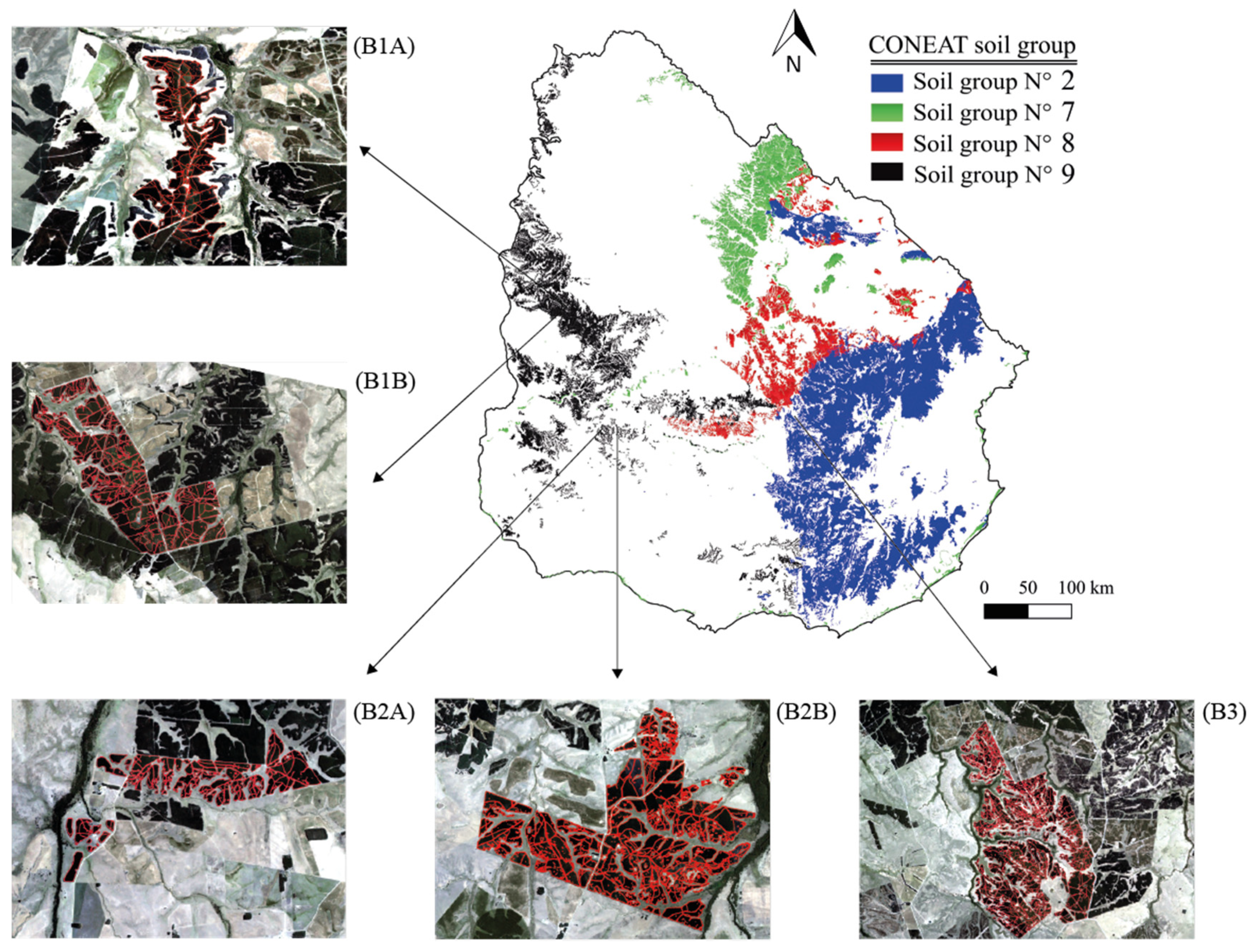
2.1. Study Area

This study was conducted in Uruguay across plantations owned by Forestal Oriental SA company, representing a total area of 2468 ha (Figure 1). Three zones were established (Figure 1): sites B1A and B1B, covering 861 ha (43°13′97″S–64°24′78″W, hereafter Guichon); sites B2A and B2B, covering 870.1 ha (63°07′44″S–52°22′64″W, hereafter Trinidad); and site B3, covering 716.9 ha (63°44′33.05″S–63°95′58″W, hereafter Sarandí del Yi).
The study zones have a temperate subtropical climate, with a mean annual temperature of 18 °C and a mean annual rainfall ranges between 1300 and 1400 mm [15]. According to the National Commission for Agroeconomic Studies of the Land (CONEAT) classification, the predominant soils at three locations were characterized by low and middle fertility, an A horizon 40–60 cm in depth, weak structure, a low to medium level of organic matter, slopes between 1–5%, sandy to loam-silt texture, and moderately-slow to slow permeability.

2.2. Field Data

In May–June 2018, 151 plots with a radius of 10 m (314.16 m2), were established using a systematic sampling design according to traditional inventory procedures within the E. grandis and E. dunnii mono-species plantations selected. In each plot, the diameter at breast height (1.3 m above ground level, cm) (dbh), stand density (N, trees ha−1), basal area (G, m2 ha−1) and total height (H, m) of all trees with a dbh greater than or equal to 7 cm were measured using a caliper (Haglöf Mantax, Långsele, Sweden) and Vertex III hypsometer. The silvicultural conditions together with the state of structure of the forest were defined using the following stand parameters: basal area per hectare (G), number of trees per hectare (N), quadratic mean diameter (dg), mean arithmetic diameter (dm), Assmann dominant height (Ho) and mean arithmetic height (Hm). For above ground biomass (AGB) and total volume (TV) estimations, equations developed by Hirigoyen (unpublished data [16]) based on dbh and total height (Hm), were used at the tree level. These equations are as follows:
For Eucalyptus dunnii:
AGB =   0.091 dbh 2.285 Hm 0.473  
TV = 0.00004 dbh 2.089 Hm 0.862
For Eucalyptus grandis:
AGB = dbh 2 ( 0.656 + 0.0005 Hm )
TV = 0.00002 dbh 1.871 Hm 1.233
The AGB and TV of the plots were computed by aggregating the individual values; a summary of the measurements made in the sample plots is presented in Table 1. The location of the center of each plot was mapped with sub-meter accuracy using post-processed, differentially corrected GPS data collected with a Trimble geo Explorer 3000 unit (Trimble Navigation Ltd., Sunnyvale, CA, USA).

2.3. Airborne LiDAR Data Acquisition and Processing

ALS data was collected in March 2018, covering a total of 2468 hectares using a Riegl VUX-1 laser scanner installed on an autogyro helicopter, at a flight altitude of 110 m above ground level, a pulse repetition rate of 550 kHz, an angular step width of 0.0687° and a FOV of 55°. The resulting point density was 40 pulses m2 (Table S1, Supplementary Material). The plots were geo-referenced in the WGS84 UTM 21 coordinate system. The planimetric x and y coordinates as well as ellipsoidal height values were recorded for all echoes.
All LiDAR point clouds were checked and processed with the software FUSION [17], and this generated four products: digital terrain model (DTM), digital surface model (DSM), canopy height model (CHM) and the LIDAR metrics used in this research. The Catalog tool was used to ensure the quality of the products created from the point clouds, evaluating various characteristics of the LIDAR data, as well as the continuity of coverage and the correct pulse return density. Areas without coverage were excluded from the study. The GroundFilter algorithm was applied to identify and remove the returns that hit the ground surface. Afterwards, a DTM with a pixel size of 1 m2 was created using these filtered points, through the GridSurfaceCreate function. The Clipdata tool was used to normalize the heights and ensure that the z coordinate corresponds to the height above ground. The Polyclipdata tool was applied to select the LIDAR points falling within the field sample plots [18]. Cloudmetrics and Grid metrics tools were used to build LIDAR metrics within the sample plots and to produce the same metrics over the LIDAR tiles at 17.7 m resolution (equivalent to a plot of ~314 m2), respectively. The LIDAR height distributional parameters (Table S2, Supplementary Material) were treated as independent variables.

2.4. Variable Selection and Statistical Analysis of the Parametric Methods

A Pearson correlation test was used to recognize highly correlated predictor variables; variables with a p-value > 0.05 were removed. Furthermore, before discarding them, we looked for correlations between the excluded variables with the target variables (Ho, TV and AGB), to fit simple linear regressions. To determine the best combinations of predictive variables, the regsubsets function (leaps package [19]) in R [20] was used. We used the Mallows Cp statistic to determine the best subsets. This compares the sum of squares error (SSE) for a reduced model with p parameters, with the mean square error of the full model (MSEfull) for a N number of samples. Models with low Cp values are generally similar to those with higher adjusted R-squared values. This criterion was selected to determine the optimal model, since it favors parsimonious models [21]. By default, regsubsets reports the best eight-variable model [22], and we used the nvmax to compare the maximum number of predictor variables that optimized Cp and the adjusted coefficients of determination.
After selecting the best set of variables, predictive models were built using forest inventory variables and LIDAR metrics. Simple and multiple linear regressions were fitted, as well as exponential, logarithmic and power transformations, considering all possible combinations. The nlsLM function from the package minpack.lm [23], a modified version of nonlinear least-squares incorporating the Levenberg-Marquardt algorithm, was used. For linear models, we used the lm function to define the prospective models, and weighted regression (using weighted least squares) was applied if heteroscedasticity was detected by ncvTest (a score test for non-constant error variance) from the car package.

2.5. Variable Selection and k-NN Models

Before the implementation of the k-NN algorithm, a multicollinearity analysis was carried out to reduce data redundancy. It was performed using the Variance Inflation Factor (VIF). Collinear variables were deleted and independent variables were selected considering a VIF >10 as the critical threshold [24], using the varSelection function from yaImpute [25] in the R package. The varSelection function keeps only those variables that strengthen the imputation process [25]. VarSelection calculates the generalized root mean square distance (grmsd) each time variables are added to an imputation algorithm. Based on several studies that have shown that the RF approach achieves better results compared to other imputation methods [26]; in this study, the k-NN models were implemented employing the RF distance metric.
After the selection of the variables, raw data were divided into training (70% of the input data) and validation (30% of the input data) sets. With the selected variables, model fitting was computed by the yai and impute.yai functions from yaimpute package [25], applied to the training set. The k-NN value (k) varied for each imputation, calculating the root-mean-square error value for each one. The k value that minimized the RMSE within the validation dataset was selected. The k-value varied for each imputation, and the one minimizing RMSE value was selected. Then, the k-NN imputations were adjusted and compared with the best selected parametric model, using reliability measures obtained in cross-validation [8].

2.6. fModel Assessment and Validation

To determine the goodness of fit, the R² adj was used during the model development stages. Simple linear regressions relating the observed and predicted values were assessed using the determination coefficient (R2) to evaluate non-linear models [26]. To analyze the relative quality of each model, the Akaike information criterion (AIC) was calculated. Model performance for the distinct approaches was evaluated based on the estimation errors, using the root-mean-square error (RMSE) and the RMSE normalized by the observed mean of the dependent variables (nRMSE, %) [26]. Thus, RMSE represents the absolute value of the error and nRMSE indicates the relative value of the error with respect to the average at the stand level.
We used R2, RMSE, and nRMSE to compare non-parametric and parametric models since, when reporting model performance the correlation between predictions and observations, should be provided along with the RMSE [26].
Cross-validation was carried out using the same data as in the fitting calculating the residuals of the i-th observation [27,28]. The sum of squares of the eliminated residues (PRESS, predicted residual error sum of squares) was used to calculate the root-mean-square-error for cross-validation (RMSEcv). The close values of RMSEcv and RMSE indicate that the model does not overfit the data and has a good predictive behavior [29].

2.7. Segmentation Method

Stand segmentation was developed, using an algorithm based in a non-parametric estimator: Mean Shift (MS), with Orpheo ToolBox (OTB) software for QGIS [30]. The MS was applied to segment the image and it can automatically detect the number of segments. In OTB three parameters were specified: spatial radius, to define the neighborhood; range radius, to define the interval in spectral space; and the minimum size of the regions that will remain after the grouping to cover all segmentation possibilities [31]. Based on the forest production (biomass and pulpwood), we used two combinations of stand silvicultural variables to define and group the LIDAR data within a single segment: (i) AGB and Ho; and (ii) TV and Ho. With this data, a two-band raster was created for both combinations (AGB and Ho; TV and Ho).
OTB segmentation was compared to that performed by a trained human operator considering the differences between species, tree ages, and values of ABG and TV. The objective was to define homogeneous areas with an optimal area of 3 hectares and a minimum of 1 hectare for: (i) TV and Ho; (ii) AGB and Ho. These silvicultural variables were selected to identify and group LiDAR data in a single support, since forest harvest takes into account wood production (volume or biomass), and Ho is used as an indicator of the quality of the forest site.

2.8. Unsupervised Evaluation of the Segmentation Method

Unsupervised evaluation (UE) was used for segmentation evaluation, based on expert knowledge. This procedure allows the results to be more efficient and less subjective compared to supervised methods [32,33]. In UE methods, each segment should be internally homogeneous and should be distinguishable from other segments [33]. UE involves calculation of intersegment homogeneity and heterogeneity measures and the aggregation of these values into a global value, thus, UE with the minimum global value is selected as the optimal segmentation [34,35]. We considered the global intra-segment homogeneity and inter-segment heterogeneity based on the variance weighted and Moran’s Index (MI) combined in a global score (GS) for measuring the quality of resulting segmentation [14]. GS is defined as the sum of the normalized weighted variance (wVar) and the normalized MI, according to [33], and has been widely used due to its simplicity of calculation, understandability, and effectiveness [36]. As there was more than one layer in each image, GS values were averaged according to the number of bands [14]. Weighted variance was calculated for each segment as follows:
w V a r = i = 1 n a i * v i i = 1 n a i
where n is the total number of segmentations, vi is the variance and ai is the area of segment i.
Moran’s index was calculated as follows:
M I = n i = 1 n j = 1 n w i j ( y i y ¯ ) ( y j y ¯ ) i = 1 n ( y i y ¯ ) 2 ( i j w i j )
where n is the total number of segmentations, wij is a measure of the spatial proximity, yi is the mean spectral value of segment i and y ¯ is the mean spectral value of the image. Each weighted wij is a measure of the spatial adjacent regions [37]. MI and wVar were both normalized by rescaling to a similar range (0–1). The optimal segmentation has low variance and low spatial autocorrelation; this means that a lower average GS indicates better results [14]. GS ranges between 0 and 2; where a value close to zero shows a low weighted variance and a low MI value [14,36]. GS was calculated as follows:
GS = wVarnorm+ MInorm
where wVarnorm is the normalized weighted variance and MInorm is the normalized Moran’s index.

3. Results

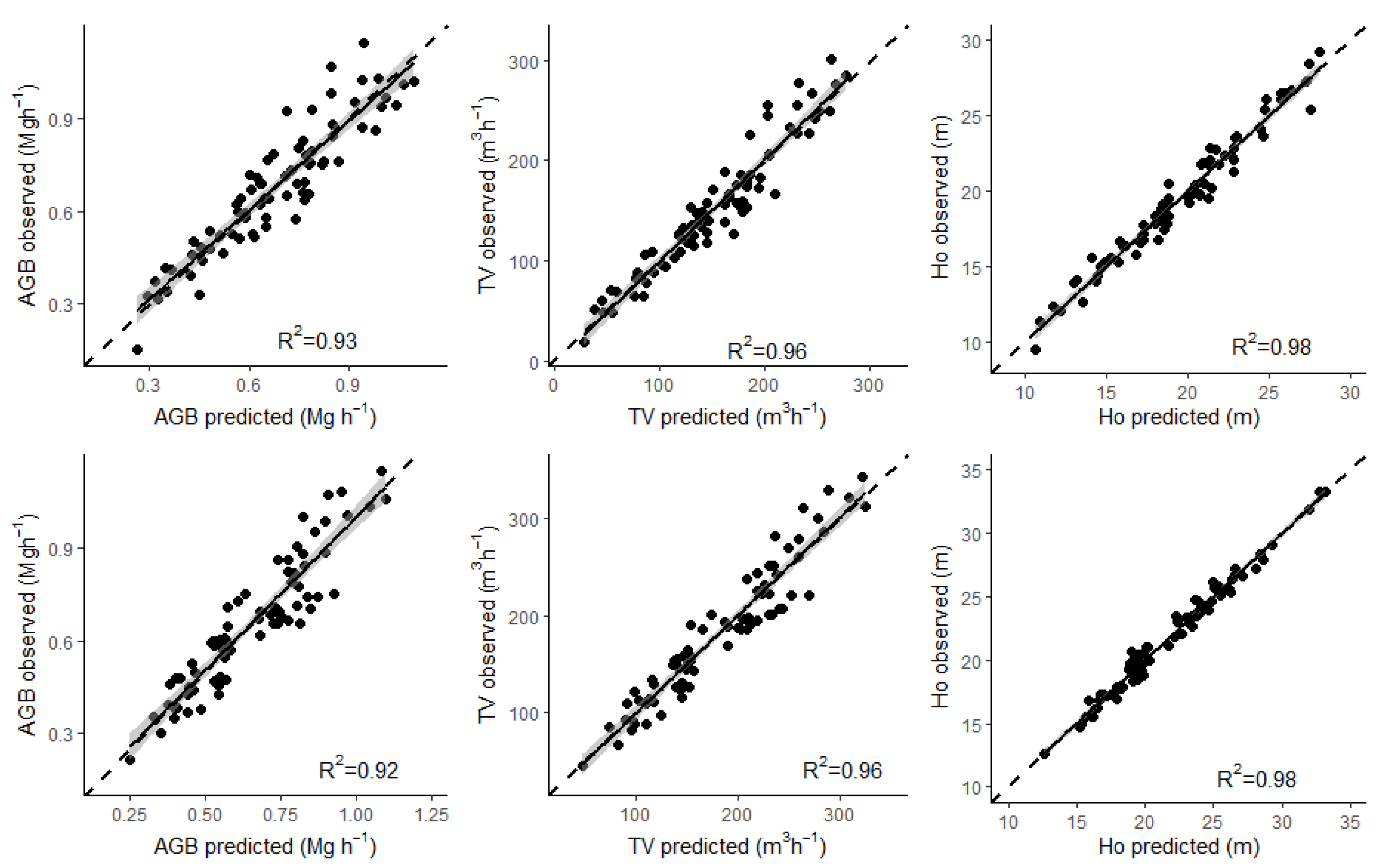
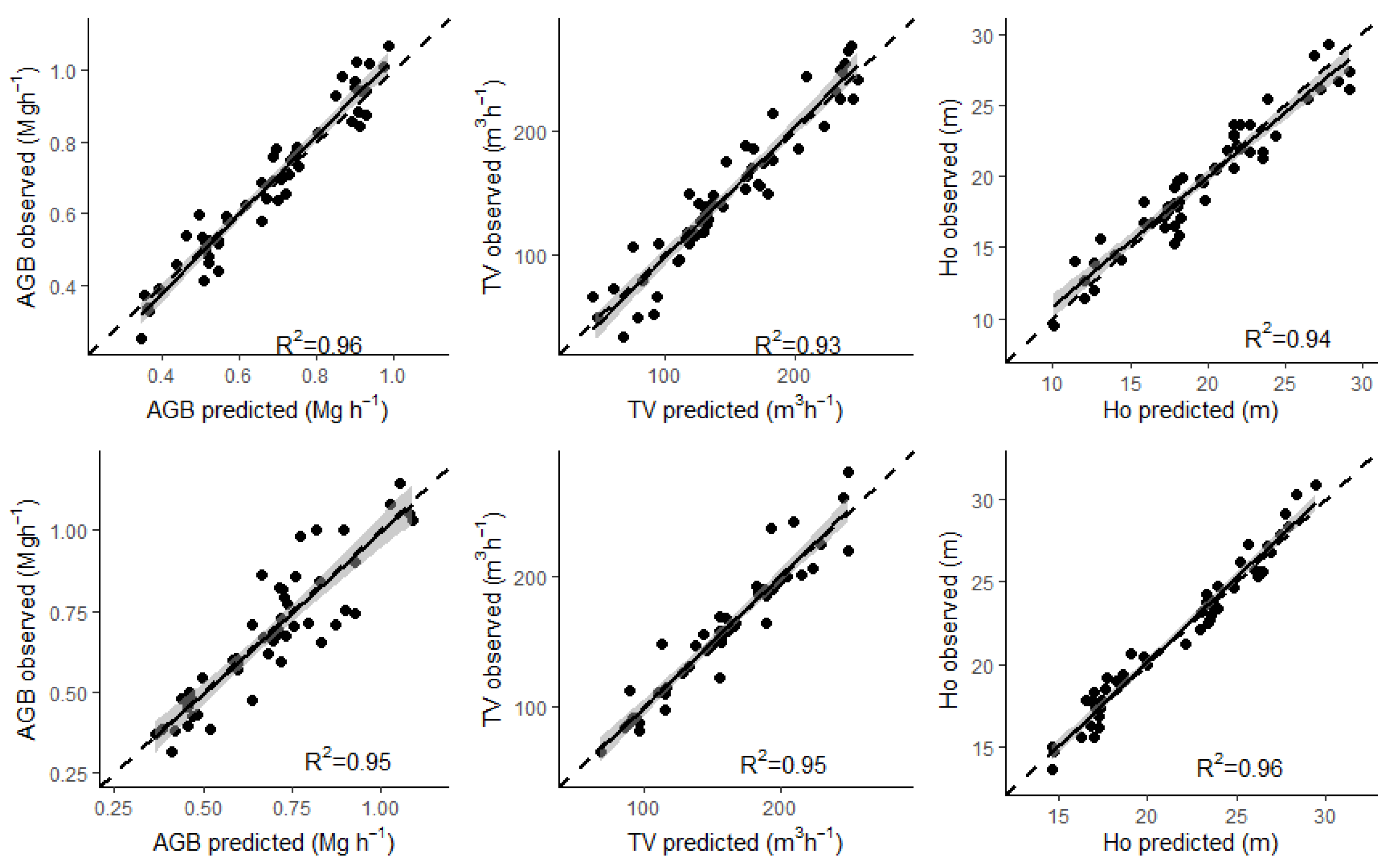
3.1. Parametric and Non-Parametric Models for Ho, TV and AGB

For E. dunnii, eight candidates’ LIDAR metrics were selected after performing multicollinearity and Pearson’s correlation tests, while for E. grandis nine LiDAR metrics were selected (Figures S1 and S2 in Supplementary Material show the selected metrics and their correlations with Ho, TV and AGB). Allometric simple linear or non-linear equations (applying the chosen metrics) were tested, using weighted least squares (WLS) to balance correlated regressor variables in multiple regression. The optimal weights that homogenized the residues and improved ncvTest were used as weight functions. Only simple linear models yielded significant parameters (p < 0.05) (candidate models, ordered by goodness of fit, are displayed in Table S3, Supplementary Material).
Models selected for E. grandis included Height percentile 99th (Elev.P99) for predicting Ho, and Height percentile 70th (Elev.P70) for predicting TV and AGB; they had determination coefficient (R2) values of 0.98, 0.96, and 0.92, respectively. For E. dunnii, models including the variables Height percentile 90th (Elev.P90) for Ho and Height percentile 75th (Elev.P75) for TV and AGB models, R2 values were 0.98, 0.96 and 0.93, respectively. In all cases, predicted values were in near-perfect agreement with the observed measurements (with R2 values higher than 0.92). The Shapiro–Wilk test and ncvTest showed that both normality and homogeneity of the residues were achieved. Scatter plots of the predicted values of Ho, TV and AGB versus the real data are shown in Figure 2.

3.2. Imputation AGB, TV and Ho Models and Their Precision
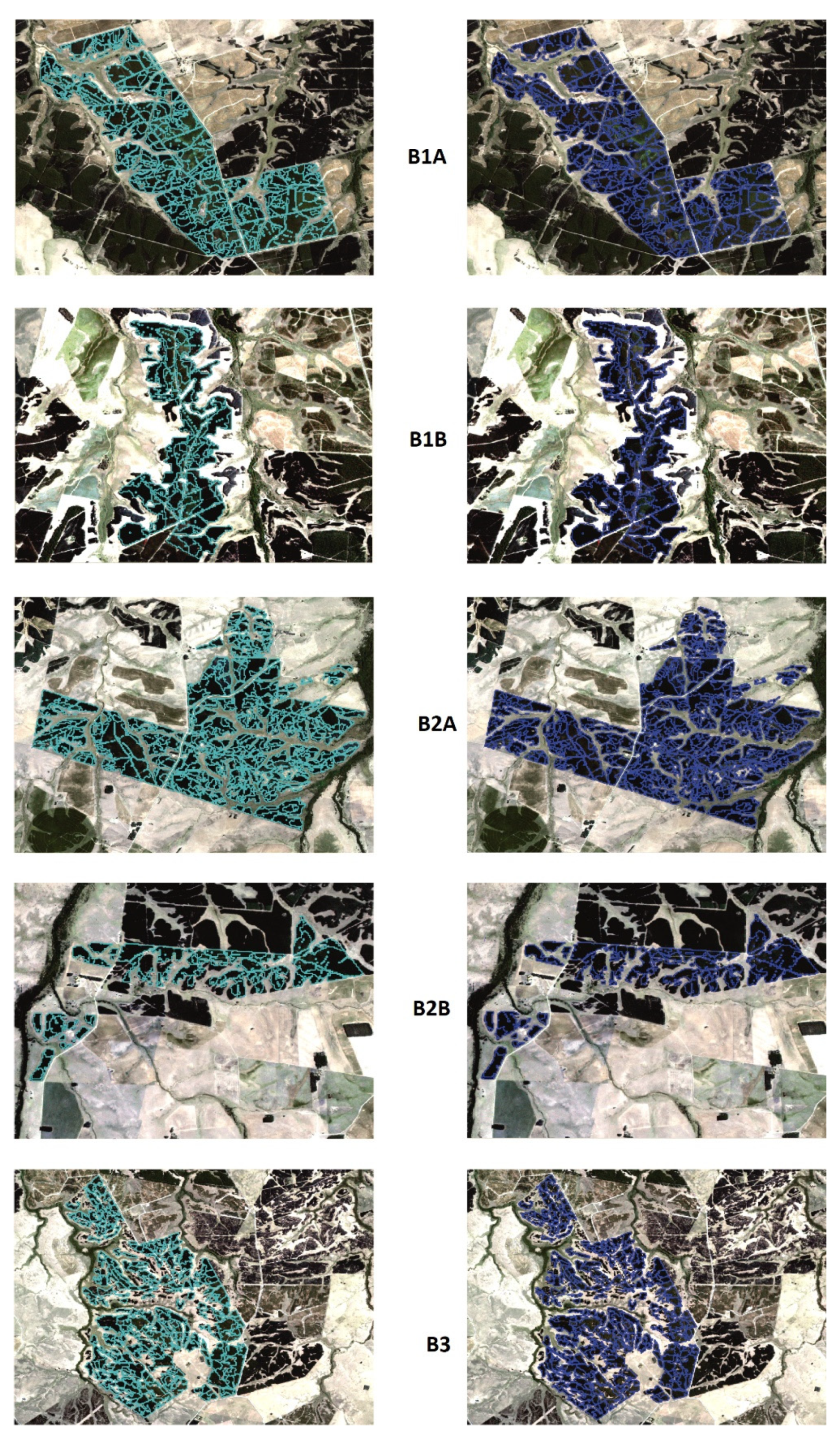
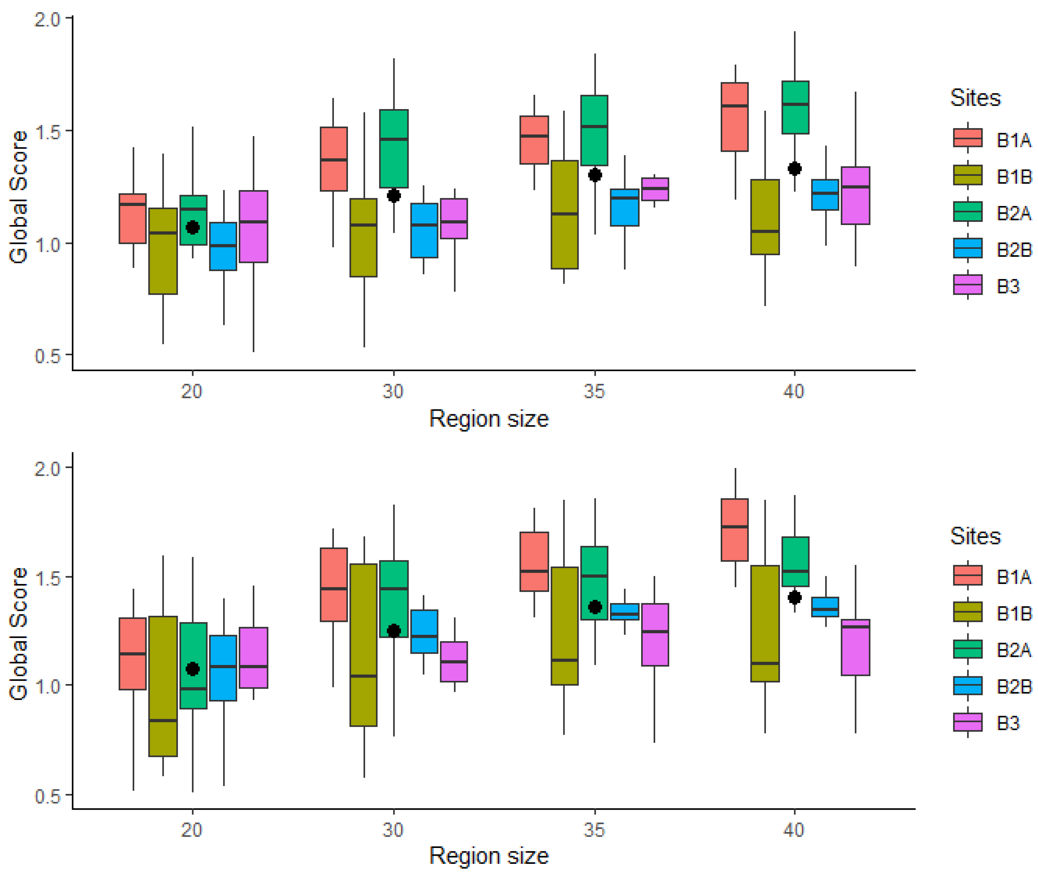
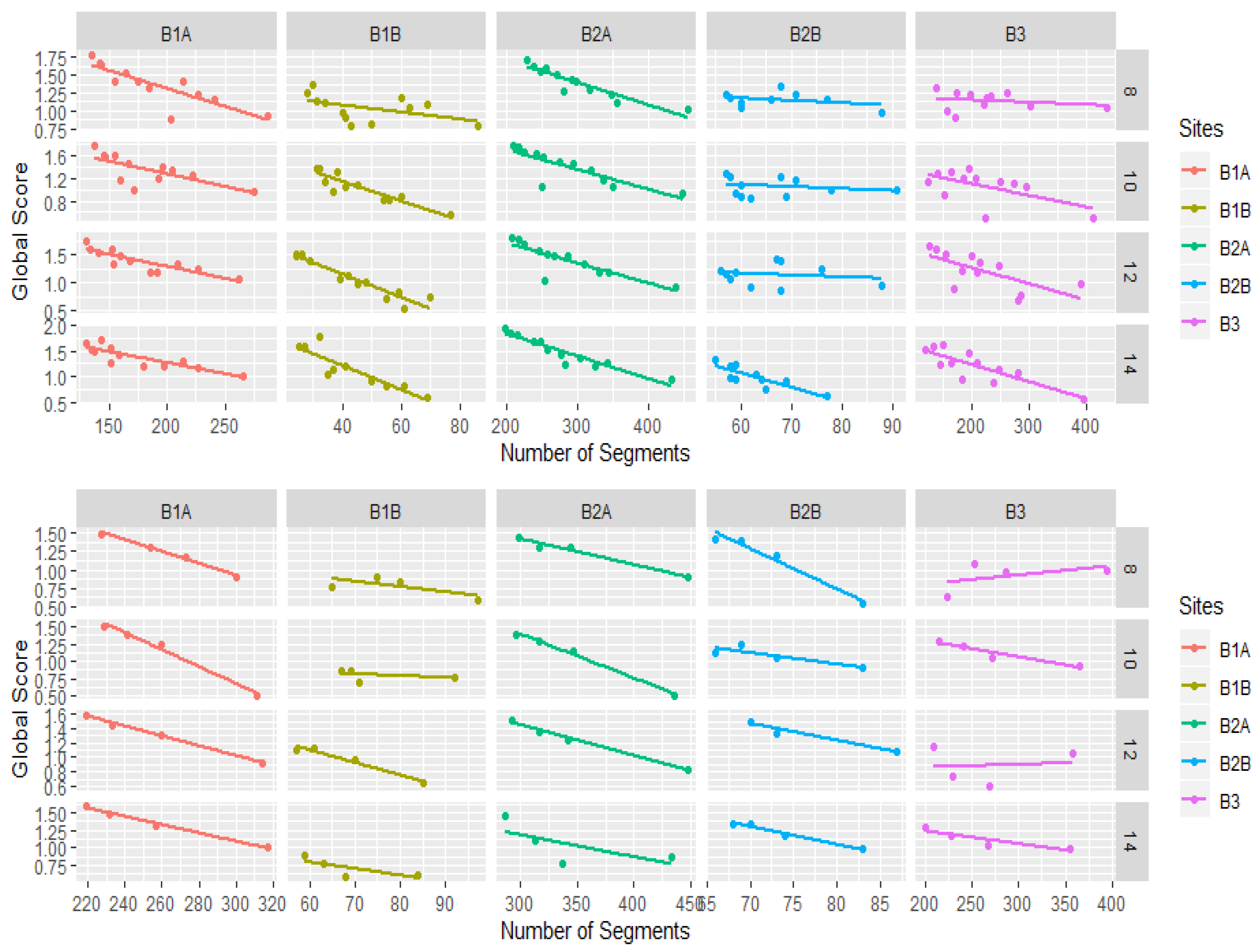
After applying the multicollinearity analysis and the correlation test to the candidate LIDAR metrics, the remainder were not highly correlated and were used as inputs in the varSelection function. Metrics selected to be included in the imputation model as predictor variables for Ho, AGB and TV, according to generalized root mean square distance (gmsd) statistics, are shown in Table 2. The LiDAR-derived predictor metrics for AGB models in E. dunnii were: height percentile 75th (Elev.P75); all returns above mode/Total first returns * 100 (ARA2/TFR); percentage first returns above mean (PFRAM); and elevation mode (Elev.MO). For E. grandis, the LiDAR-derived metrics were: Elev.P75, canopy relief ratio (CRR); and Elev.MO. The LiDAR-derived metrics selected as predictors in TV models for E. dunnii were: Elev.P75; ARA2/TFR and Elev.MO. For E. grandis, the LiDAR-derived metrics were: Elev.P75, percentage first returns above mode (PFRAMO); elevation maximum (Elev.MAX) and all returns above height break (ARA2). The models fitted for Ho of E. dunnii included the LIDAR-derived predictor metrics Elev.P75 and ARA2; those of E. grandis included Elev.P75, Elev.Max and CRR.
The results of imputed models are given in Table 3. We included cross-validation as accuracy estimation methods; this allowed us to analyze the predictive capacity of each model. Results show that metrics expressing middle or upper-middle percentiles of LIDAR heights (Elev.75) were included as predictors in all models for both species. All models followed a similar trend, with RMSE and nRMSE% being slightly higher compared to fitting statistics, for all variables. However, RMSE and nRMSE were lower for Ho of E. grandis. For Ho, TV and AGB, cross-validation of the selected models yielded average RMSE and nRMSE% values of 1.5 m and 10%; 25 m3 ha−1 and 18%; and 120 Mg ha−1 and 17%, respectively, for both species.
Plots of model predictions versus the observed data are shown in Figure 3. Relationships between observed and estimated AGB, TV, and Ho consistently exhibited R2 values exceeding 0.93.

3.3. Segmentation

The results of applying OTB segmentation in the delimitation of the forest stand, described by the number of segments created, varies with the combination of minimum size, range radius and spatial radius (see Tables S4 and S5, Supplementary Material). Sites B1A, B1B, B2A and B2B were established due to the distance between the original stands (see Figure 1). Table 4 shows the selected segmentation for the sites, and these values are clear in the field delineation of Figure 4.
Table 5 shows the total number of segments obtained by manual segmentation and for the Orpheo ToolBox OTB algorithm. Manual segmentation produced more segments than OTB for all sites except B2A. For site B2A, OTB by TV segmentation produced 3% more than AGB segmentation. AGB segmentation yielded more segments than TV (B1A = 3.4%, B2B = 5.9%). For B3, OTB segmentation for AGB and TV produced almost the same results in both cases, producing 25.8% fewer segments than with manual segmentation.
To evaluate the effects of region size on the GS values from different combinations of range, boxplots of spatial radius versus region size were assessed (Figure 5) for AGB and TV. For small region sizes, the behavior of the GS was quite uniform either applying segmentations obtained using TV or with those obtained using AGB. Differences among sites increased as the size of the region increased. The largest difference was observed for a size of 40, in both the TV and AGB segmentations. B1B had greater variability of GS than the rest of the sites for AGB and TV, this being more pronounced for AGB. For the TV segmentations, site B2A had the highest values of GS, for all sizes, while for the AGB segmentations site B1A had the highest values of GS, for all sizes; in both cases, this was more evident in the larger regions.
The relationship between segment number and global score is shown in Figure 6 when the range radius was fixed at 4.

4. Discussion

Our study has compared the performance of parametric and non-parametric methods for estimating AGB, TV, and Ho, using LIDAR data at the stand level). AGB, TV and Ho are key inputs in models used to estimate the stand gross annual increment [38]. Then, we assessed the best combination of AGB-Ho and TV-Ho for stand segmentation. These results permit the generation of accurate Eucalyptus forest-stand segmentations using the mean shift segmentation method, which may be used to improve the programing of forestry and harvesting.

4.1. Assmann Dominant Height, Total Volume, and Above Ground Biomass Modeling

Ho is required for empirical models that are based on the site index (SI). The SI and height are generally used as an indicator of the quality of the forest site and for estimating the volume of standing trees [39]. ALS sensors have been widely used for the determination of forest parameters including AGB and TV [40,41], being a suitable technology for forest inventory and management [39].
In this study, we developed parametric and non-parametric models to estimate Ho, AGB and TV. Regarding LiDAR metric selection, for parametric models, the best predictors of Ho were related to the highest percentiles of the point cloud (Elev.90 and Elev.99) consistently as descriptors of dominant height. LIDAR height metrics, such as height percentiles, are frequent in studies that use LIDAR data for forest inventory [33,42]. However, using percentiles as unique independent variables will give the same result for stands with the same mean dominant height but different stand density. For volume and biomass models, the middle or upper-middle percentiles of the point cloud (Elev.70 and Elev.75) had greater importance. These upper-middle statistics of the point cloud report the tree crown properties [43,44], and have been used to explain other tree variables (e.g., stem diameter through) [45]. Hence, the 70th and 75th percentiles are expected to replace dbh in the equations developed to calculate the variables from field data (Equations (1)–(4)). Similar achievements were attained by other authors when modeling the above ground biomass in Eucalyptus stands [46,47].
For non-parametric models, all the k-NN models included at least one variable related to height metrics (Elev.P75, Elev.MAX, Ele.MO) and the shape of the height distribution (CRR), and most of the models included a variable related to cover metrics (PFRAM, ARMO). According to previous studies, the combination of height and density in the canopy metrics represents a description of the vertical structure of the forest stand [47]. Our k-NN models for AGB, TV, and Ho in the two Eucalyptus species included only one variable related to the upper-middle percentiles of the point cloud (Elev.75), as well as variables related to the density of the canopy (ARA2/TFR, PFRM, CRR, ARMO). The results demonstrate that Elev.75 is potentially useful for improving forest models.
The percentage of returns above a certain height with respect to total returns is a metric that serves to characterize the forest cover. When modeling the dominant height (Ho), it will be more correlated with the highest percentiles of the height, since they are more related to tree height. The AGB and TV were calculated using equations including diameter (d) and height (TH) as the independent variables. Models generated on this study integrated high percentiles of forest canopy, representing tree height, and intermediate percentiles (e.g. p75 or the mode of heights) representing the diameter. Additionally, models included variables related to tree density, such as canopy relief ratio and first return above median, which could be substituted by the percentage of returns above 2 m since they belong to the same family of LiDAR metrics that provide a similar explanation for forest canopy.
The most common estimation methods of Ho, TV and AGB in forest inventories using LIDAR are ordinary simple regression methods (e.g., least squares regression) and non-parametric methods (e.g., RF, SVM and the nearest neighbor-based methods) [46]. Our results showed that both WLS and k-NN are suitable methods for predicting AGB, TV and Ho using LIDAR data. In our study, in the TV models, R²-adj was 0.91 with Elev.70 for E. grandis and 0.92 with Elev.75 for E. dunnii, whereas the model with Elev.75 and the model with Elev.70 as the regressor took second place for E. grandis and E. dunnii, respectively. The AGB models had the same single independent variable as the TV models, for both species, but the R²-adj values were lower: 0.86 and 0.85 for E. grandis and E. dunnii, respectively. In the Ho models, Elev.99 (R²-adj 0.98), for E. grandis, and Elev.90 (R²-adj 0.96), for E. dunnii, were selected as independent variables. The graphical trends of the residuals showed that the models were not affected by problems of homogeneity of variances. The accuracy of the models is confirmed by the low relative values of nRMSE, and by the values of cross-validation ( R M S E c v ) . Additionally, the closeness of the RMSEcv and RMSE values indicates that the models have good predictive value.
Comparison of the results of the selected parametric models with those of the non-parametric models show small differences. Our results suggest that the k-NN (with RF distance metric) models performed better (as indicated by R2, RMSE and RMSEcv) for TV and AGB. This has been reported also in most of the other studies that have compared parametric and non-parametric methods [47]. However, the Ho parametric model had better performance than the k-NN model, for both species, possibly explained by the strong correlation of the former with the highest percentiles. the differences between the two methods are small.

4.2. Segmentations

The normalized MI values, and the normalized weighted variance included in the global score of the segmentations indicate that OTB detected homogeneous stand well, in agreement with previous research [14,33,36]. The implementation of OTB for the delimitation of forest stands has proved to be simpler, more efficient and of similar precision compared to other more complex methods. Visually and quantitatively, the results show that the proposed segmentation method yielded high-quality segmentation when compared to manual segmentation. Thus, OTB segmentation could be used to automatically segment Eucalyptus stands, producing spatial stands that an expert could identify in a similar way to traditional photography (Figure 4). The results are consistent with other studies that use LIDAR for the automation of the delimitation of the stand applied in the field of forest inventory [11,33,39].

4.3. Applications in Forest Management

In this study, we have provided a framework for using LIDAR data to predict AGB, TV and Ho at the stand-level, employing parametric and non-parametric methods. We have shown that the use of regression models and non-parametric segmentation methods can provide more reliable AGB and TV distribution maps with lower error levels.
The implementation of a segmentation method such as OTB, improve time processing by increasing the area covered and maximizing the labor efficiency. The segmentation proposed on this study defines stands using TV or AGB with a similar site index (by Ho). This allows planning activities such as road construction, localized harvests or future plantations.
Additionally, forest stand delimitation, based on these silvicultural variables and OTB method, worked well. This approach may contribute to better forest management through (i) greater success on growth and yield projections by improving the estimates of stand variables ensuring the development and implementation of growth and production models; (ii) assist the yield optimization according to the size of the stand, achieving a more efficient and homogeneous planning in terms of volume and products, (iii) the selection of stands for harvest, using a simple and inexpensive method that is regulated by the production estimates of the stands themselves, (iv) site classification is potentially improved by projecting Ho over the complete forest cover.
Having stand variables prediction models based on LiDAR metrics allows its application in large areas based on the calibration plots. Forest managers can manage more efficiently if they have wood production estimates that cover the entire area and not just those measured in traditional inventories. Forest management plans, based on prediction models, as well as stand segmentation based on these predictions, contribute to achieve coherence between inventory data and the final products harvested for the entire area covered by ALS. OTB is an economically more profitable solution than other specific forest management software, which allows forest producers to have a planning tool.

5. Conclusions

This study provides tools that allow the improvement of precision in two fundamental steps of forest stock quantification: stand variables modeling (above ground biomass, total volume and dominant height), using LIDAR and the delimitation of stand structure based on unsupervised evaluation. The parametric methods had better performance for Ho, and the non-parametric methods delivered better results in terms of precision and bias for TV and AGB. High-spatial-resolution maps of those variables can be created from LIDAR data once robust models have been developed which were used to stand segmentation. The segmentation methodology proposed here provide a cost-effective and easy-to-update model for the generation of maps of AGB or TV for harvest tasks, based on rasters derived from LIDAR metrics. These tools, based on LIDAR metrics, allow forest managers to improve the decision-making process on forestry based on forest inventory, above ground biomass and total volume information for strategic management purposes (improving records of carbon sequestration rates and AGB fluxes, for example). It also exposes the need to continue advancing and promoting the application of ALS data for the inventory of forest plantations of Eucalyptus spp. in Uruguay.

Supplementary Materials

The following are available online at https://0-www-mdpi-com.brum.beds.ac.uk/2072-4292/12/23/3947/s1. Figure S1: Selected LIDAR-derived metrics and its correlation with total volume (TV, above ground biomass (AGB) and Assmann’s dominant height (Ho) to Eucalyptus dunnii. Figure S2: Selected LIDAR-derived metrics and its correlation with, total volume (TV), above ground biomass (AGB) and Assmann’s dominant height (Ho) to Eucalyptus grandis. Table S1: Riegl VUX-1 specification. Table S2: Summary of the LIDAR-derived metrics computed including abbreviations and categories. Table S3: Models for estimating total volume (TV, m3 ha−1), total above ground biomass (AGB, Mg ha−1) and Assmann´s dominant height (Ho, m) of Eucalyptus grandis and Eucalyptus dunnii in Uruguay using LIDAR metrics. R2-adj = adjusted coefficient of determination, RMSE = root mean squared error, nRMSE = normalized root mean squared error, AIC = Akaike information criterion. Table S4: Selected Normalized variance (Vnorm), normalized Moran’s Index (MInorm) and global scores (GS) for all spatial radius, range radius and minimum size of the region segmentations with theirs resulting number of segments. OTB mean shift segmentation approach for TV. Table S5: Selected Normalized variance (Vnorm), normalized Moran’s Index (MInorm) and global scores (GS) for all spatial radius. range radius and minimum size of the region segmentations with theirs resulting number of segments, OTB mean shift segmentation approach for AGB.

Author Contributions

Conceptualization, A.H., C.R.-C. and R.M.N.-C.; methodology, A.H., M.A.V.-M. and R.M.N.-C.; formal analysis, A.H., M.A.V.-M. and J.F.; investigation, A.H., M.A.V.-M., C.R.-C. and R.M.N.-C.; data curation, A.H., C.R.-C. and M.A.V.-M.; writing—original draft preparation, A.H., M.A.V.-M. and C.R.-C.; writing—review and editing, A.H., R.M.N.-C. and J.F.; supervision, R.M.N.-C. All authors have read and agreed to the published version of the manuscript.

Funding

This research received no external funding.

Acknowledgments

The authors thank the Instituto Nacional de Investigaciones Agropecuarias (INIA-Uruguay) for supporting our research work and for help during the fieldwork. We are particularly grateful for the support of Roberto Scoz, Demian Gomez, Zenia Barrios and Gustavo Balmelli (INIA), Mariano Blanco, Santiago Heguaburu, Carola Odone and José Carlos de Mello (FOSA). R.M.N.-C. acknowledges the ISOPINE (UCO-1265298) and ESPECTRAMED (CGL2017-86161-R) projects for methodological support. We acknowledge the institutional support of the University of Cordoba-Campus de Excelencia CEIA3. We also thank the ERSAF group and, particularly. Cristina Acosta and Antonio Ariza. for their assistance during this research. We thank David Walker for his revisions of the different versions of this manuscript, and the anonymous referees for their comments and corrections.

Conflicts of Interest

The authors declare no conflict of interest.

References

  1. Hawbaker, T.J.; Gobakken, T.; Lesak, A.; Trømborg, E.; Contrucci, K.; Radeloff, V. Light detection and ranging-based measures of mixed hardwood forest structure. For. Sci. 2010, 56, 313–326. [Google Scholar]
  2. Hościło, A.; Lewandowska, A. Mapping Forest Type and Tree Species on a Regional Scale Using Multi-Temporal Sentinel-2 Data. Remote Sens. 2019, 11, 929. [Google Scholar] [CrossRef] [Green Version]
  3. Naesset, E. Determination of mean tree height of forest stands using airborne laser scanner data. ISPRS J. Photogramm. Remote Sens. 1997, 52, 49–56. [Google Scholar] [CrossRef]
  4. González-Ferreiro, E.; Arellano-Pérez, S.; Castedo-Dorado, F.; Hevia, A.; Vega, J.A.; Vega-Nieva, D.; Álvarez-González, J.G.; Ruiz-González, A.D. Modelling the vertical distribution of canopy fuel load using national forest inventory and low-density airbone laser scanning data. PLoS ONE 2017, 12, e0176114. [Google Scholar] [CrossRef]
  5. Zhang, Z.; Cao, L.; Mulverhill, C.; Liu, H.; Pang, Y.; Li, Z. Prediction of Diameter Distributions with Multimodal Models Using LiDAR Data in Subtropical Planted Forests. Forests 2019, 10, 125. [Google Scholar] [CrossRef] [Green Version]
  6. Nelson, R. How did we get here? An early history of forestry lidar1. Can. J. Remote Sens. 2013, 39, S6–S17. [Google Scholar] [CrossRef] [Green Version]
  7. Bouvier, M.; Durrieu, S.; Fournier, R.A.; Renaud, J.-P. Generalizing predictive models of forest inventory attributes using an area-based approach with airborne LiDAR data. Remote Sens. Environ. 2015, 156, 322–334. [Google Scholar] [CrossRef]
  8. Gregoire, T.G.; Næsset, E.; McRoberts, R.E.; Ståhl, G.; Andersen, H.-E.; Gobakken, T.; Ene, L.; Nelson, R. Statistical rigor in LiDAR-assisted estimation of aboveground forest biomass. Remote Sens. Environ. 2016, 173, 98–108. [Google Scholar] [CrossRef]
  9. Garcia-Gutierrez, J.; Gonzalez-Ferreiro, E.; Riquelme-Santos, J.C.; Miranda, D.; Dieguez-Aranda, U.; Navarro-Cerrillo, R.M. Evolutionary feature selection to estimate forest stand variables using LiDAR. Int. J. Appl. Earth Obs. Geoinf. 2014, 26, 119–131. [Google Scholar] [CrossRef]
  10. O’Hara, K.L.; Nagel, L.M. The stand: Revisiting a central concept in forestry. J. For. 2013, 111, 335–340. [Google Scholar] [CrossRef] [Green Version]
  11. Dechesne, C.; Mallet, C.; Le Bris, A.; Gouet, V.; Hervieu, A. Forest stand segmentation using airborne lidar data and very high resolution multispectral imagery. Int. Arch. Photogramm. Remote Sens. Spat. Inf. Sci. ISPRS Arch. 2016, 41, 207–214. [Google Scholar] [CrossRef]
  12. Haara, A.; Haarala, M. Tree species classification using semi-automatic delineation of trees on aerial images. Scand. J. For. Res. 2002, 17, 556–565. [Google Scholar] [CrossRef]
  13. Sanchez-Lopez, N.; Boschetti, L.; Hudak, A. Semi-Automated Delineation of Stands in an Even-Age Dominated Forest: A LiDAR-GEOBIA Two-Stage Evaluation Strategy. Remote Sens. 2018, 10, 1622. [Google Scholar] [CrossRef] [Green Version]
  14. Johnson, B.; Xie, Z. Unsupervised image segmentation evaluation and refinement using a multi-scale approach. ISPRS J. Photogramm. Remote Sens. 2011, 66, 473–483. [Google Scholar] [CrossRef]
  15. Castaño, J.P.; Giménez, A.; Ceroni, M.; Furest, J.; Aunchayna, R.; Bidegain, M. Caracterización Agroclimática del Uruguay 1980–2009; Serie Técnica INIA 193; Instituto de Investigaciones Agropecuarias: Montevideo, Uruguay, 2011. [Google Scholar]
  16. Andrés, H.; Rafael, N.; Jorge, F.; Maurizio, B.; Cecilia, R. Modelling Taper, Total and Merchantable Stem Volume Considering Stand Density Effects to Eucalyptus Grandis and Eucalyptus Dunnii in Uruguay. iForest 2020, in press. [Google Scholar]
  17. McGaughey, R.J. FUSION/LDV: Software for LiDAR Data Analysis and Visualization. February 2013–FUSION Version 3.30; USDA Forest Service, Pacific Northwest Research Station, University of Washington: Seattle, WA, USA, 2013. [Google Scholar]
  18. Silva, C.A.; Klauberg, C.; Hudak, A.T.; Vierling, L.A.; Liesenberg, V.; Bernett, L.G.; Scheraiber, C.F.; Schoeninger, E.R. Estimating Stand Height and Tree Density in Pinus taeda plantations using in-situ data, airborne LiDAR and k-Nearest Neighbor Imputation. An. Acad. Bras. Ciênc. 2018, 90, 295–309. [Google Scholar] [CrossRef]
  19. Lumley, T. Using Fortran Code by Alan Miller. Leaps: Regression Subset Selection, R Package Version 2.9; Available online: http://CRAN.R-project.org/package=leaps2009 (accessed on 1 August 2020).
  20. R Development Core Team. R Core Development Team A Language and Environment for Statistical Computing: Reference Index Version 3.5.1; R Development Core Team: Vienna, Austria, 2013. [Google Scholar]
  21. Mallows, C.L. Some comments on Cp. Technometrics 2000, 42, 87–94. [Google Scholar]
  22. Zhao, F.; Guo, Q.; Kelly, M. Allometric equation choice impacts lidar-based forest biomass estimates: A case study from the Sierra National Forest, CA. Agric. For. Meteorol. 2012, 165, 64–72. [Google Scholar] [CrossRef]
  23. Elzhov, T.V.; Mullen, K.M.; Spiess, A.-N.; Bolker, B.; Mullen, M.K.M.; Suggests, M. Package ‘minpack.lm.’ Title R Interface Levenberg-Marquardt Nonlinear Least-Sq. Algorithm Found MINPACK Plus Support Bounds’. 2016. Available online: https://cran.rproject.org/web/packages/minpack.lm/minpack.lm.pdf (accessed on 20 November 2020).
  24. Quinn, G.P.; Keough, M.J. Experimental Design and Data Analysis for Biologists; Cambridge University Press: Cambridge, UK, 2002; ISBN 1139432893. [Google Scholar]
  25. Crookston, N.L.; Finley, A.O. YaImpute: An R Package for kNN Imputation. J. Stat. Softw. 2008, 23, 1–16. [Google Scholar] [CrossRef] [Green Version]
  26. Zald, H.S.J.; Wulder, M.A.; White, J.C.; Hilker, T.; Hermosilla, T.; Hobart, G.W.; Coops, N.C. Integrating Landsat pixel composites and change metrics with lidar plots to predictively map forest structure and aboveground biomass in Saskatchewan, Canada. Remote Sens. Environ. 2016, 176, 188–201. [Google Scholar] [CrossRef] [Green Version]
  27. Knapp, N.; Fischer, R.; Huth, A. Linking lidar and forest modeling to assess biomass estimation across scales and disturbance states. Remote Sens. Environ. 2017, 205, 199–209. [Google Scholar] [CrossRef]
  28. Kohavi, R. A Study of Cross-Validation and Bootstrap for Accuracy Estimation and Model Selection. Int. Jt. Conf. Artif. Intell. 1995, 2, 1137–1143. [Google Scholar]
  29. Andersen, H.-E.; McGaughey, R.J.; Reutebuch, S.E. Estimating Forest Canopy Fuel Parameters Using LIDAR Data. Remote Sens. Environ. 2005, 94, 441–449. [Google Scholar] [CrossRef]
  30. Qgis, D.T. QGIS Geographic Information System, Open Source Geospatial Foundation. 2009. Available online: https://0-scholar-google-com.brum.beds.ac.uk/scholar_lookup?title=QGIS%20Geographic%20Information%20System&author=QGIS%20Development%20Team&publication_year=2009#d=gs_cit&u=%2Fscholar%3Fq%3Dinfo%3AK9pErfIkywoJ%3Ascholar.google.com%2F%26output%3Dcite%26scirp%3D0%26hl%3Des (accessed on 20 November 2020).
  31. Comaniciu, D.; Meer, P. Mean shift: A robust approach toward feature space analysis. IEEE Trans. Pattern Anal. Mach. Intell. 2002, 24, 603–619. [Google Scholar] [CrossRef] [Green Version]
  32. Wu, Z.; Heikkinen, V.; Hauta-Kasari, M.; Parkkinen, J.; Tokola, T. Forest Stand Delineation Using a Hybrid Segmentation Approach Based on Airborne Laser Scanning Data; Springer: Berlin/Heidelberg, Germany, 2013; pp. 95–106. [Google Scholar]
  33. Varo-martínez, M.Á.; Navarro-cerrillo, R.M.; Hernández-clemente, R. Semi-automated stand delineation in Mediterranean Pinus sylvestris plantations through segmentation of LiDAR data: The influence of pulse density. Int. J. Appl. Earth Obs. Geoinf. 2017, 56, 54–64. [Google Scholar] [CrossRef] [Green Version]
  34. Grybas, H.; Melendy, L.; Congalton, R.G. A comparison of unsupervised segmentation parameter optimization approaches using moderate-and high-resolution imagery. GIScience Remote Sens. 2017, 54, 515–533. [Google Scholar] [CrossRef]
  35. Zhang, X.; Feng, X.; Xiao, P.; He, G.; Zhu, L. Segmentation quality evaluation using region-based precision and recall measures for remote sensing images. ISPRS J. Photogramm. Remote Sens. 2015, 102, 73–84. [Google Scholar] [CrossRef]
  36. Espindola, G.M.; Camara, G.; Reis, I.A.; Bins, L.S.; Monteiro, A.M. Parameter selection for region-growing image segmentation algorithms using spatial autocorrelation. Int. J. Remote Sens. 2006, 27, 3035–3040. [Google Scholar] [CrossRef]
  37. Zhang, X.; Xiao, P.; Feng, X. An unsupervised evaluation method for remotely sensed imagery segmentation. IEEE Geosci. Remote Sens. Lett. 2011, 9, 156–160. [Google Scholar] [CrossRef]
  38. White, J.C.; Coops, N.C.; Wulder, M.A.; Vastaranta, M.; Hilker, T.; Tompalski, P. Remote Sensing Technologies for Enhancing Forest Inventories: A Review. Can. J. Remote Sens. 2016, 42, 619–641. [Google Scholar] [CrossRef] [Green Version]
  39. Mora, B.; Wulder, M.A.; White, J.C.; Hobart, G. Modeling stand height, volume, and biomass from very high spatial resolution satellite imagery and samples of airborne LIDAR. Remote Sens. 2013, 5, 2308–2326. [Google Scholar] [CrossRef] [Green Version]
  40. Böck, S.; Immitzer, M.; Atzberger, C. On the Objectivity of the Objective Function—Problems with Unsupervised Segmentation Evaluation Based on Global Score and a Possible Remedy. Remote Sens. 2017, 9, 769. [Google Scholar] [CrossRef] [Green Version]
  41. Yang, L.; Mansaray, L.R.; Huang, J.; Wang, L. Optimal segmentation scale parameter, feature subset and classification algorithm for geographic object-based crop recognition using multisource satellite imagery. Remote Sens. 2019, 11, 514. [Google Scholar] [CrossRef] [Green Version]
  42. Shao, G.; Shao, G.; Gallion, J.; Saunders, M.R.; Frankenberger, J.R.; Fei, S. Improving Lidar-based aboveground biomass estimation of temperate hardwood forests with varying site productivity. Remote Sens. Environ. 2018, 204, 872–882. [Google Scholar] [CrossRef]
  43. Matasci, G.; Hermosilla, T.; Wulder, M.A.; White, J.C.; Coops, N.C.; Hobart, G.W.; Bolton, D.K.; Tompalski, P.; Bater, C.W. Three decades of forest structural dynamics over Canada’s forested ecosystems using Landsat time-series and lidar plots. Remote Sens. Environ. 2018, 216, 697–714. [Google Scholar] [CrossRef]
  44. Næsset, E.; Økland, T. Estimating tree height and tree crown properties using airborne scanning laser in a boreal nature reserve. Remote Sens. Environ. 2002, 79, 105–115. [Google Scholar] [CrossRef]
  45. Lo, C.S.; Lin, C. Growth-competition-based stem diameter and volume modeling for tree-level forest inventory using airborne LiDAR data. IEEE Trans. Geosci. Remote Sens. 2013, 51, 2216–2226. [Google Scholar] [CrossRef]
  46. Guerra-Hernández, J.; Görgens, E.B.; García-Gutiérrez, J.; Rodriguez, L.C.E.; Tomé, M.; González-Ferreiro, E. Comparison of ALS based models for estimating aboveground biomass in three types of Mediterranean forest. Eur. J. Remote Sens. 2016, 49, 185–204. [Google Scholar] [CrossRef]
  47. Jayathunga, S.; Owari, T.; Tsuyuki, S. Digital Aerial Photogrammetry for Uneven-Aged Forest Management: Assessing the Potential to Reconstruct Canopy Structure and Estimate Living Biomass. Remote Sens. 2019, 11, 338. [Google Scholar] [CrossRef] [Green Version]
Figure 1. Location of the study sites in Uruguay soils prioritized for forestry (soil groups: 2, 7, 8, 9) and Planet satellite images (March 2018) of study sites: B1A and B1B (Guichon); B2A and B2B (Trinidad) and site B3 (Sarandí del Yi).
Remotesensing 12 03947 g001
Figure 2. Relationships between observed and predicted values for total volume (TV, m3 ha−1), total above ground biomass (AGB, Mg ha−1) and Assmann´s dominant height (Ho, m) of Eucalyptus dunnii (upper) and E. grandis (bottom) in Uruguay by parametric regression. Solid line depicts regression fit, dashed line is the 1:1 line. Correlation coefficient (R2) value is included. Shaded areas represent 95% regression confidence intervals.
Remotesensing 12 03947 g002
Figure 3. Relationships between observed and imputed values for total volume (TV, m3 ha−1), total above ground biomass (AGB, Mg ha−1) and Assmann’s dominant height (Ho, m) of Eucalyptus dunnii (upper) and E. grandis (bottom) in Uruguay by non-parametric method. Solid line depicts regression fit and dashed line shows the 1:1 line. Correlation coefficient (R2) value is included. Shaded areas represent 95% regression confidence intervals.
Remotesensing 12 03947 g003
Figure 4. Stands delineated obtained using mean shift segmentation: in sky-blue: above ground biomass; in blue: total volume by sites.
Remotesensing 12 03947 g004
Figure 5. Global scores for total volume–dominant height (top) and above ground biomass-dominant height (bottom) segmentation versus minimum size. Black points are the mean value for each size.
Remotesensing 12 03947 g005
Figure 6. Trend of global score for total volume–dominant height (top) and above ground biomass-dominant height (bottom) by number of segments and spatial radius. Range radius was fixed in 4, continued lines are smooth (lm) trends.
Remotesensing 12 03947 g006
Table 1. Silvicultural and biomass variables of Eucalyptus grandis and Eucalyptus dunnii in Uruguay: number of plot(n), stem density (N, trees ha−1); diameter at breast height (dbh, cm); basal area (G, m2 ha−1), above ground biomass (AGB, Mg ha−1), total height (TH, m), total volume (TV, m3 ha−1), and age (years). stdev: standard deviation, min: minimum, max: maximum.
Field AttributesMinMeanMaxStdev
E. grandis (n = 76)Dbh (cm)10.6515.4919.331.81
TH (m)12.5721.6933.304.46
G (m2 ha−1)8.9720.2829.794.52
AGB (Mg ha−1) 215.2653.31175213.2
TV (m3 ha−1)45.01185.37342.1267.71
Age4.56.89.51.5
N (tree ha−1)63410411336144
E. dunnii (n = 75)Dbh (cm)10.8315.2719.381.53
TH (m)9.5219.5529.224.23
G (m2 ha−1)0.7620.5133.795.41
AGB (Mg ha−1) 153.3686.71296218.2
TV (m3 ha-1)18.81154.73300.6064.49
Age4.56.38.41.2
N (tree ha−1)66910701432159
Table 2. LiDAR-derived metrics selection according to generalized root means square distance (grmsd) as predictor variables in imputation model for total volume (TV, m3 ha−1), total above ground biomass (AGB, Mg ha−1), and Assmann´s dominant height (Ho, m) of Eucalyptus grandis and Eucalyptus dunnii in Uruguay. Canopy relief ratio, CRR; elevation mode, Elev.MO; height percentile 75th Elev.P75; all returns above mode/total first returns * 100, ARA2/TFR; percentage first returns above mean, PFRAM; percentage first returns above mode, PFRAMO; all returns above height break, ARA2; elevation maximum, Elev.MAX; all returns above mode, ARAMO.
E. grandisE. dunnii
MetricsgrmsdMetricsgrmsd
AGBCRR0.461Elev.MO0.466
Elev.MO0.479ARA2/TFR0.476
Elev.P750.562PFRAM0.511
Elev.P750.547
TVElev.P750.556Elev.P750.394
PFRAMO0.567Elev.MO0.401
ARA20.568ARA2/TFR0.410
Elev.MAX0.580
HoElev.MAX0.303ARAMO0.343
CRR0.313Elev.P750.394
Elev.P750.349
Table 3. Statistics of fit and cross -validation for Assmann’s dominant height (Ho m), total volume (TV m3 ha−1), and above ground biomass (AGB mg ha−1) of Eucalyptus grandis and Eucalyptus dunnii in Uruguay. R2, coefficient of determination; RMSE, root mean squared error; nRMSE, normalized root mean squared.
E. dunnii E. grandis
RMSEnRMSER2RMSEnRMSER2
HoFit1.387.120.941.165.310.97
Cross Validation2.0010.220.901.084.980.97
TVFit18.4316.280.9320.0415.060.93
Cross Validation20.7518.150.8924.7717.440.84
AGBFit71.210.370.9670.211.890.95
Cross Validation112.217.080.8711017.090.85
Table 4. Selected normalized variance (wVnorm), normalized Moran’s index (MInorm), and global scores (GS) for all spatial radius, range radius, and minimum size of the region segmentations with theirs resulting number of segments and average areas. Orpheo ToolBox (OTB) mean shift segmentation approach was applied for the estimation of above ground biomass (AGB mg ha−1) and total volume (TV m3) of Eucalyptus grandis and Eucalyptus dunnii in Uruguay using LIDAR metrics.
SitesSpatial RadiusRange RadiusMin Size of RegionAGB BandTV BandHo BandTwo-Band AverageNumber SegmentsAverage Area (ha)
wVnormMInormGSwVnormMInormGSwVnormMInormGSwVnormMInormGS
B1A
84200.930.000.93 0.870.000.870.900.000.903002.19
8420 0.950.000.950.900.000.900.930.000.932872.28
B1B
144300.620.300.91 0.000.240.240.310.270.57683.02
12430 0.790.150.940.000.120.120.390.140.53613.36
B2A
104200.020.971.00 0.020.000.020.020.490.514361.68
10420 0.040.930.970.030.850.880.030.890.924491.63
B2B
84200.000.950.95 0.020.090.120.010.520.53831.68
14420 0.010.770.780.020.460.480.020.610.63771.81
B3
84400.500.020.53 0.380.020.400.440.020.462243.19
10440 0.440.070.510.480.010.490.460.040.502253.18
Table 5. Number of segments and average size of stand area, applying the Orfeo Tool Box algorithm and manual segmentation of above ground biomass (AGB) and total volume (TV), in Eucalyptus grandis and Eucalyptus dunnii plantations in Uruguay.
BlockTotal Block Area (ha)Segment Number ManualAverage
Segment
Area (ha)
Segment Number AGBAverage Segment
Area (ha)
Segment Number TVAverage Segment Area (ha)
B1A654.73801.723002.182872.28
B1B205.9802.57683.03613.38
B2A731.94251.724361.684491.63
B2B139.41021.37831.68771.81
B3716.63022.372243.202253.18
Publisher’s Note: MDPI stays neutral with regard to jurisdictional claims in published maps and institutional affiliations.

