Shadow Detection and Restoration for Hyperspectral Images Based on Nonlinear Spectral Unmixing


Department of Photogrammetry and Remote Sensing, German Aerospace Center (DLR), 88234 Wessling, Germany
*
Author to whom correspondence should be addressed.
Remote Sens. 2020, 12(23), 3985; https://0-doi-org.brum.beds.ac.uk/10.3390/rs12233985
Submission received: 10 November 2020
/
Revised: 28 November 2020
/
Accepted: 3 December 2020
/
Published: 5 December 2020
(This article belongs to the Special Issue Spectral Unmixing of Hyperspectral Remote Sensing Imagery)
Abstract
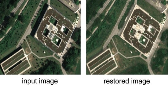
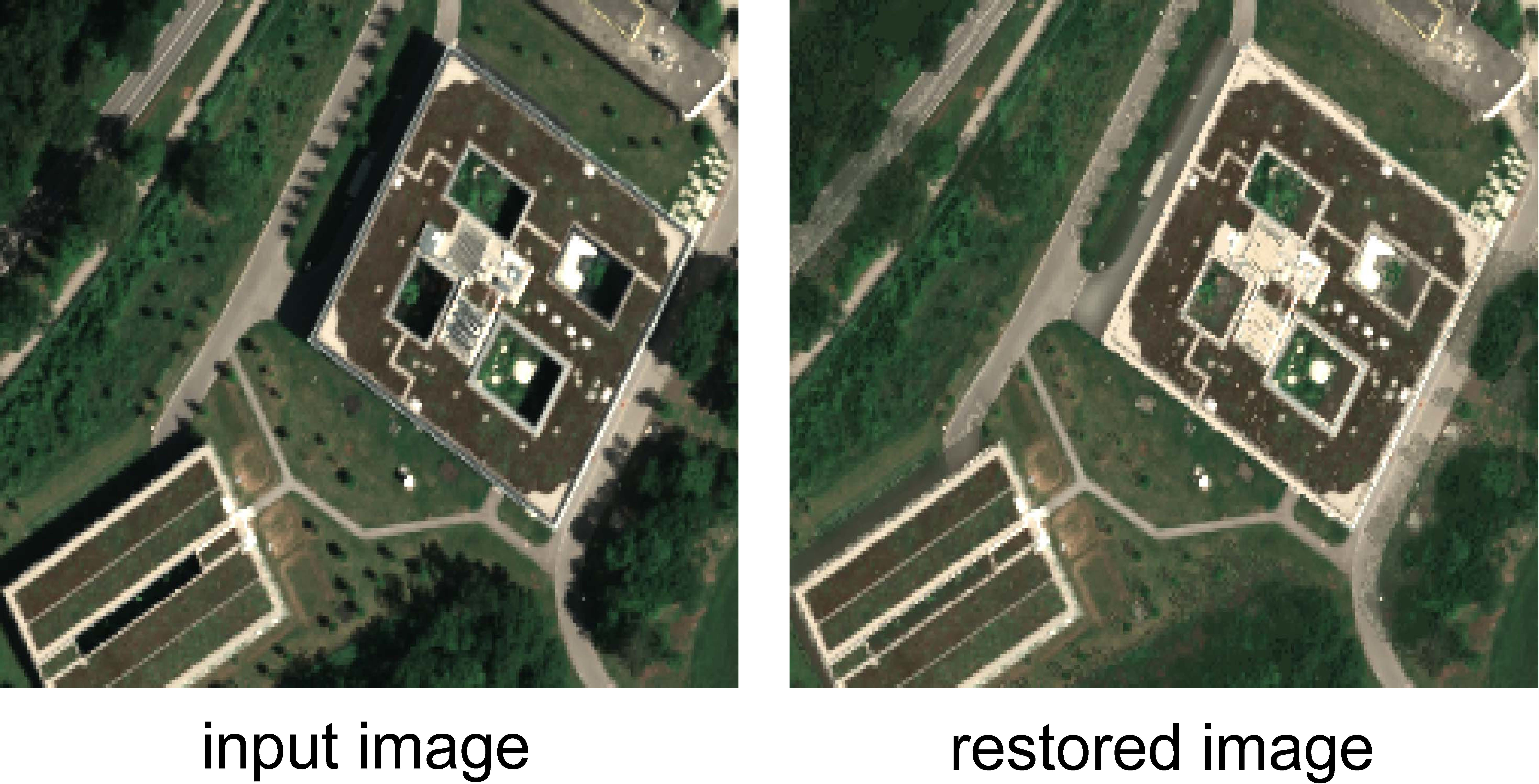
:Shadows are frequently observable in high-resolution images, raising challenges in image interpretation, such as classification and object detection. In this paper, we propose a novel framework for shadow detection and restoration of atmospherically corrected hyperspectral images based on nonlinear spectral unmixing. The mixture model is applied pixel-wise as a nonlinear combination of endmembers related to both pure sunlit and shadowed spectra, where the former are manually selected from scenes and the latter are derived from sunlit spectra following physical assumptions. Shadowed pixels are restored by simulating their exposure to sunlight through a combination of sunlit endmembers spectra, weighted by abundance values. The proposed framework is demonstrated on real airborne hyperspectral images. A comprehensive assessment of the restored images is carried out both visually and quantitatively. With respect to binary shadow masks, our framework can produce soft shadow detection results, keeping the natural transition of illumination conditions on shadow boundaries. Our results show that the framework can effectively detect shadows and restore information in shadowed regions.
1. Introduction
In images with high spatial resolution, shadows are frequently visible [1]. According to the principle of formation, these consist of cast shadow and self-shadow [2]. When an object occludes the direct solar illumination outdoors, self-shadow occurs on the part of the object with no direct solar illumination. Cast shadow, which this paper considers, is projected instead on nearby objects, and consist of umbra and penumbra [2]: the former is the shadowed region where the direct sun illumination is completely blocked by the object, while the latter is the shadowed region where the direct solar illumination is partly blocked due to the finite extension of the light source. As shadow pixels lack direct sun illumination, their computed reflectances can be incorrect without a shadow restoration process. The inaccurate reflectance values in shadowed regions hinder image analysis, such as classification and target detection. Therefore, it is of great interest to restore the correct reflectance values in shadowed areas.
Previous works studying shadow detection or shadow removal from optical images use optical earth observation data, including RGB, multispectral, and hyperspectral images [2,3,4]. Imaging spectrometer data, also referred to as hyperspectral (We are aware that the terms “imaging spectroscopy” and “imaging spectrometer data” are more exact than “hyperspectral imaging” and “hyperspectral data”, respectively, and therefore should be preferred. Nevertheless, in this paper we also use the term “hyperspectral” for the sake of briefness [5].), provide spectral measurements with near-continuous acquisition wavelengths. These data convey rich spectral information related to the physical properties of ground materials and their chemical composition, compared with RGB and multispectral images, and are extremely valuable for different remote sensing applications [6].
Correspondingly, shadow detection and removal methods have been proposed specifically or generally for one among these three categories of data [2,3,4]. Shadow detection is frequently used as a preliminary step before shadow removal. Many works have investigated shadow detection methods and detailed reviews can be seen in [1,7]. One category of simple but popular shadow detection methods sets threshold values in a given data space to detect shadow regions [3,8]. In addition to RGB bands, near-infrared (NIR) bands are often used, because they are more sensitive to shadows [7,9]. One drawback of these methods is selecting suitable thresholds [1]. In addition, sunlit dark pixels and shadowed bright pixels can be wrongly detected [7]. Authors in [10] applied water masks in order to alleviate the impact from water regions. A second category of methods maps RGB images to color spaces insensitive to lighting conditions, such as Hue-Saturation-Value (HSV), Hue-Chroma-Value (HCV), deriving back RGB combinations after local brightness alterations [11,12,13]. A third category of methods studies the geometry and light sources of the scene (ray tracing) [14,15]. These algorithms depend on the availability and accuracy of geometrical data [16]. Other solutions consider physical information. Authors in [17,18] assume that shadow is a zero reflectance endmember and detect shadows through a matched filter. These methods can confuse shadows with materials characterized by low albedo. Authors in [19] compute the proportion of a pixel relative to skylight by considering illumination conditions in shadowed areas [19]. Furthermore, some works study shadow detection based on unsupervised or supervised machine learning methods. Authors in [4] apply K-means clustering, considering the shadow as one output class. In supervised methods, training samples of sunlit and shadowed pixels are selected, then classification methods are applied to separate shadowed from sunlit pixels [20]. The performance of machine-learning-based methods may depend on differences between ground objects and the selection of training samples. Recently, shadow detection based on deep learning has been proposed [21,22]. These methods usually require training data containing input RGB images and their corresponding ground-truth binary shadow masks. In addition, some methods solve shadow detection and restoration in the same framework [23,24]: we will come back to them in the discussion of shadow restoration algorithms.
Numerous methods have been proposed for removing shadows from RGB images. One family of algorithms operates in the gradient domain [23,25,26]. Those methods detect shadow boundaries, where gradient values are large, then restore images by nullifying the gradients on shadow boundaries. In order to locate shadow boundaries, different methods of computing illumination invariant images have been proposed. A second category of methods is based on color space transformation [27]. Those methods aim to transform an image from the RGB color space to other color spaces, e.g., HIS (hue, intensity, and saturation), HSV (hue, saturation, and value), HCV (hue, chroma, and value), YIQ (luminance, in-phase, and quadrature), or YCbCr (luminance, the blue-difference chroma component, and the red-difference chroma component), so that pixel values in the transferred space are insensitive to illumination changes. Following a different approach, other works focus on correlating sunlit regions with shadowed regions at pixel or object level. In [12], the authors apply three correction models (Gamma model, Linear model, and histogram matching) on paired sunlit and shadowed regions. In later works, shadow and sunlit regions are matched based on texture similarity before applying correction models [28]. Nevertheless, it proves challenging to automatically correlate regions in large and complex scenes. In addition, it is difficult to apply a single correction model to an entire image indiscriminately [3], because the radiometry of the image can vary largely in the spatial domain.
Finally, approaches relying on the inclusion of other types of external data have been proposed to tackle these problems. For instance, depth data are applied through non-local matching, with the assumption that pixels with similar chromaticity, normals, and spatial locations have similar colors [29]. Recently, deep learning methods have become popular. The method proposed in [30] learns the most relevant features in a supervised manner using multiple convolutional deep neural networks (ConvNets). Based on the shadow mask result, shadows are removed in a Bayesian framework. Authors in [31] propose an automatic and end-to-end deep neural network (DeshadowNet) for shadow detection and removal. This method requires a large amount of training data.
Compared with RGB images, shadow detection and removal in multispectral and hyperspectral images bring specific challenges and opportunities. On the one hand, the high spectral resolution of imaging spectrometer data provides valuable information for shadow removal; on the other hand, it is difficult to exactly recover the spectral information for all the spectral bands of the dataset in shadowed pixels.
Earlier works have investigated shadow removal specifically on multispectral or hyperspectral images. One category [4] transforms hyperspectral data to hyperspherical coordinates in order to suppress the difference between shadowed and lighted pixels of the same material. Additionally, since hyperspectral data contain near-continuous spectra, shadow pixels are matched with sunlit pixels by minimizing the spectral distances between them [32,33]. Recently, authors in [34] use the spectral angle distance as reconstruction cost function [35] in a deep learning framework, so that the network can learn brightness-independent encodings. Authors in [24] developed a deep-learning-based framework to detect shadows and retrieve urban land-cover classes from multispectral imagery. The network is trained on a shadow semantic annotation database, where 103 image patches are labeled with various types of shadows and six land-cover classes. Moreover, Lidar data are used as an additional data source when compensating shadow regions in the hyperspectral image [36,37], as Lidar provides the precise geometry of a scene. An illumination invariant image is generated in [36] through the physical process with the aid of Lidar data, while shadowed regions are restored in [37] using a precise digital surface model.
A different family of algorithms relies on spectral unmixing, in which a pixel is decomposed as a linear combination of constituent spectra, i.e., endmembers, and relative fractions, i.e., abundances [38]. Given that endmembers are spectra of pure materials in an image, spectral unmixing assumes multiple materials to be present in a single resolution cell, and analyzes the percentage of each endmember present in the pixel. Conventional spectral unmixing methods regard shadows as either a single “black” endmember, whose spectral values at all wavelengths are zeros [17], or a “shade” endmember, whose spectral values are largely lower than other endmembers at all wavelengths [39]. Authors in [40] propose a shadow compensation method based on linear unmixing with the assumption that the construction of the spectral scatter plot in shadows is analogues to that in non-shadow areas within a two-dimension spectral mixing space. Shadowed regions have lower radiance values with respect to sunlit targets of the same material, but they should not be treated independently. Hence, when conducting spectral unmixing, it should preferable to treat shadow areas with different physical assumptions. Authors in [41] investigate the situation where a grass region is shadowed by trees. Shadowed regions are therein modeled with a bilinear model, by multiplying the reflectances of shadow and tree endmembers. In addition, spectral angle distances [32] have been also used together with unmixing in de-shadowing tasks. The unmixing process is conducted in [42] separately in sunlit and shadowed regions. Two groups of endmembers are then matched through minimum spectral angle distance, followed by a shadow restoration process using sunlit endmembers. In addition to relying on spectral angle distances, authors in [40] match sunlit endmembers with shadowed endmembers of the same materials, under the assumption that the construction of the spectral scatter plot in shadows is analogs to the one in sunlit areas for a two-dimension spectral mixing space. Finally, a nonlinear mixture model has been proposed in [43] to detect shadow pixels, by modeling optical interactions of light rays between the light source and the observer.
To the best of our knowledge, the following are the main open problems concerning shadow detection and removal in hyperspectral images.
- –
- –
- –
- –
- –
- Shadow restoration may introduce spectral distortion in sunlit pixels.
- –
- –
The proposed framework could contribute to some extent to the reported open problems. In this paper, as an extension of our previous work [46,47], we propose a shadow detection and restoration method for high-resolution hyperspectral reflectance images based on nonlinear unmixing, considering both umbra and penumbra. Our proposed framework restores reflectance data in shadowed regions without the requirement of shadow detection results as an additional input. In addition to the restored images, the framework computes soft shadow detection maps ranging from 0 to 1 which, unlike binary masks, yield a natural restoration on the shadow boundaries. As an optional step, our method iteratively refines the initial spectral library by automatically including undetected materials. We tested the proposed framework on airborne data acquired by an imaging spectrometer in the visible (VIS) and near-infrared (NIR) spectral ranges.
This paper is organized as follows. In Section 2, we propose a shadow detection and restoration method based on radiative transfer and a non-linear unmixing model. Section 3 introduces test data acquired by an imaging spectrometer and Section 4 analyzes experimental results, followed by detailed discussions in Section 5. Finally, we conclude our work and give directions for possible future extensions in Section 6.
2. Methodology
The proposed framework for simultaneous shadow detection and removal is reported in Figure 1. The input consists of one hyperspectral image and a spectral library consisting of pure spectra from sunlit regions, i.e., sunlit endmembers. The initial spectral library should not contain any endmember related to shadows or penumbra regions, while it should include similar materials with large differences in absolute magnitude. In order to fully satisfy these requirements, we manually select pure spectra from sunlit regions in this paper. The output of the framework consists of a sunlit factor map and a restored shadow-free hyperspectral image.
Direct and diffuse solar irradiances are the main illumination sources for outdoor scenes [48]. Sunlit regions receive both of them, while the umbra in shadowed regions receives only the diffuse solar irradiance due to occlusion. Despite the different illumination conditions between sunlit and shadowed regions, reflectance as a physical property remains theoretically unchanged for a material. In reality, though, the observed reflectances in shadowed regions are much lower than those in sunlit regions for the same material. This is caused by the fact that differences in illumination conditions in the scene are usually ignored when computing reflectance values.
Consequently, we model the spectrum of a shadowed material given the spectrum of the same material under sunlight (Section 2.1). Subsequently, we regard both sunlit and shadowed spectra as endmembers and construct a nonlinear mixture model (Section 2.2). Finally, sunlit spectra weighted by all abundance values are used to compute the restored shadow-free image (Section 2.2). The proposed framework generates as an additional output a soft shadow detection result, i.e., sunlit factor map, by residual analysis of the mixture models (Section 2.3). The sunlit factor map can locate sunlit pixels, where values of the restored image are then replaced by their input pixels.
2.1. Shadowed Spectra Model
Direct and diffuse solar irradiances are two major illumination sources [48] and they are assumed constant across a small scene. Assuming the ground targets to be Lambertian, the reflectance of a sunlit pixel can be written as:
where is the radiance of the sunlit pixel at wavelength , is the direct solar irradiance at the sunlit pixel at wavelength , and is the diffuse solar irradiance at the sunlit pixel at wavelength .
For shadowed pixels, the illumination sources are diffuse solar irradiance and multiple reflections from the surrounding objects. In contrast, the computation of reflectances, i.e., atmospheric correction, violates the realistic illumination conditions in shadowed pixels, if it does not consider topography information. In other words, the atmospheric correction step assumes that the illumination sources of shadowed pixels are the same with sunlit pixels, i.e., direct and diffuse solar irradiance. Hence, the observed reflectance for a shadow pixel can be represented as in Equation (2). We use the term “observed” as Equation (2) follows the computation of the atmospheric correction step. Nevertheless, such observed reflectance is incorrect in terms of physics.
Accordingly, is the radiance of the shadowed pixel contributed at wavelength by the linear part, i.e., diffuse solar irradiance, while is the radiance of the shadowed pixel at wavelength contributed by the nonlinear part, i.e., multiple reflections of direct solar irradiance caused by surrounding objects.
Modeling nonlinear effects for spectral unmixing has been explored for decades (see reviews in [38,49]). In this paper, we model using the Fan model [50], which forms nonlinear interactions through the multiplication of reflectances using abundances as coefficients:
where p is the number of materials (endmembers) in one pixel, is the reflectance of the i-th sunlit material (endmember) at wavelength , and is the i-th abundance corresponding to .
After combining Equations (1)–(3), can be written as:
The ratio indicates the proportion of the diffuse solar irradiance to the direct solar irradiance on the ground surface. For the same time and location, this ratio becomes smaller at longer wavelengths. In addition, this ratio depends on atmospheric conditions such as aerosol, humidity, and dust content [51]. Consequently, we model the ratio as a power function . By assuming atmospheric conditions to be constant across a single airborne image, all parameters ,, and are constants. Another free parameter F, representing how much diffuse irradiance a pixel receives out of a certain direct solar irradiance, is estimated pixel-wise. The described ratio is then computed as:
where is a wavelength, , , are positive quantities, and F ranges from 0 to 1.
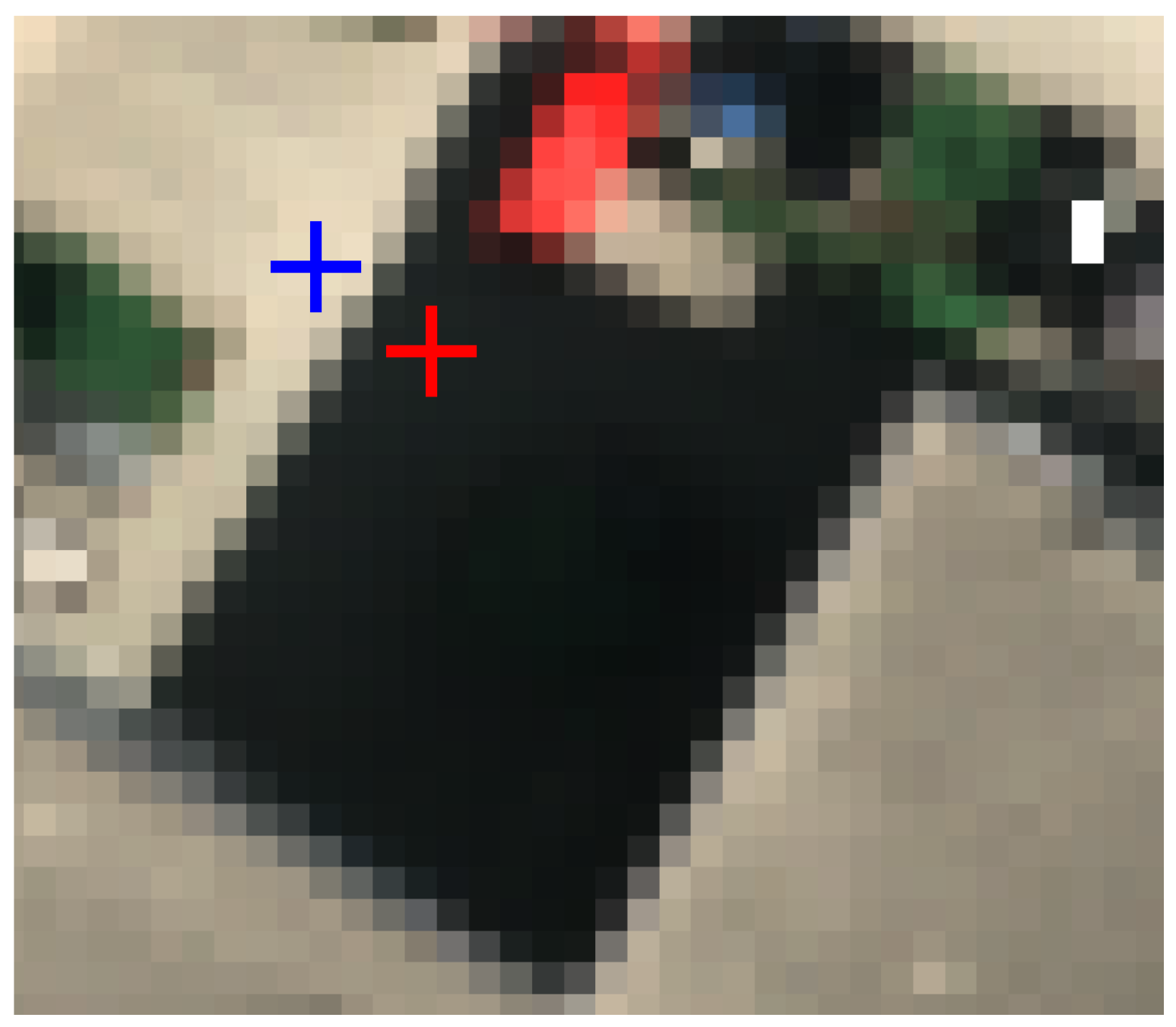
The parameters , , and in Equation (6) can be solved by using manually selected pairs of sunlit spectra, i.e., and shadowed spectra, i.e., , for selected materials in the scene. In high-resolution images, shadow boundaries appear between sunlit and shadowed regions and may span more than one pixel, as shown in Figure 2. As an example in Figure 2, the selected pixels in each pair should therefore be located close to but not directly on the shadow boundary.
2.2. Nonlinear Mixture Model
We write Equation (6) in vector form, in order to solve for all wavelengths simultaneously and construct a nonlinear mixture model to allow more materials to be present in one pixel. Note that is the i-th sunlit endmember, where , with p the total number of endmembers, the i-th abundance corresponding to the i-th sunlit endmember, and the i-th abundance corresponding to the i-th shadowed endmember. Given an i-th sunlit endmember , a corresponding shadowed endmember can be written as:
Then both and can be regarded as endmembers (spectra related to pure pixels). For one pixel , we construct a nonlinear mixture model through Equation (8). When solving this equation, we additionally apply a total generalized variation (TGV) algorithm [52] to the parameter F for spatial smoothness in an iterative manner. In the first iteration, we solve all unknown parameters in Equation (8). After that, F is spatially filtered through the TGV algorithm, and then used as a known parameter in the second iteration.
where , , and . In order to account for physical considerations, abundances are positive values. In addition, we apply the sum-to-one constraint by assuming that all endmembers are recognized for each pixel. Since spectral values of shadowed pixels are much lower than those of sunlit pixels, the sum-to-one constraint assures that shadowed pixels yield large abundances of shadowed endmembers, instead of small abundances of sunlit endmembers.
With and representing respectively the abundance of shadowed and sunlit endmember for the same material, the shadow restoration result for a pixel with B spectral bands is computed as:
2.3. Sunlit Factor Map
From Section 2.1 and Section 2.2, endmembers can be either sunlit or shadowed .
We decompose Equation (8) into two sub-equations by separating the and terms, resulting in Equations (10) and (11). After spectral unmixing, the reconstructed images using Equations (8), (10), and (11) are noted as , , and , respectively. Both sunlit and shadowed pixels can be reconstructed with Equation (8), which contains both and terms. Shadowed pixels can be reconstructed with Equation (10), while sunlit pixels can be reconstructed with Equation (11) with small reconstruction errors through spectral unmixing. Therefore, in a B-dimensional space spanned by B spectral bands, the Euclidean distance between and is small in shadowed pixels and large in sunlit pixels. On the other hand, the Euclidean distance between and is large in shadowed pixels and small in sunlit pixels. We therefore compute a sunlit factor map pixel by pixel according to the equation . The sunlit factor map ranges from 0 to 1. In this paper, we use two fixed thresholds set as and , respectively. When sunlit factor values are smaller than , pixels are assumed to be pure shadowed pixels. When sunlit factor values are larger than , pixels are assumed to be pure sunlit pixels.
3. Dataset
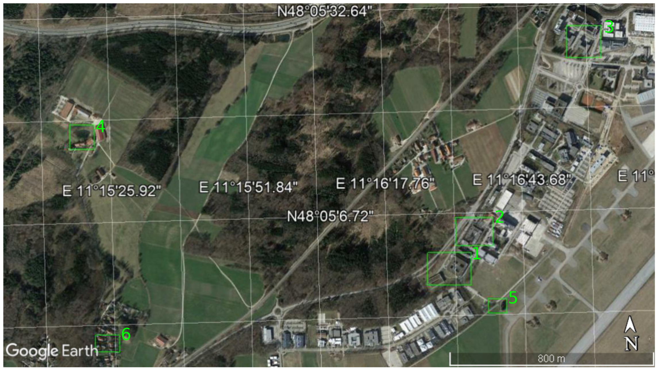
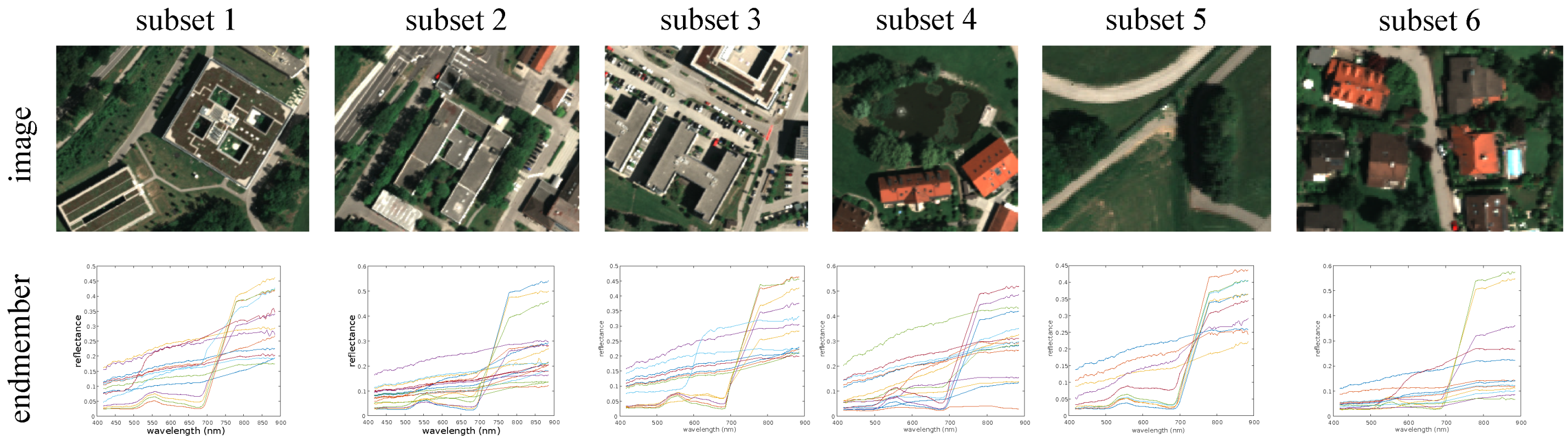
We analyze six subsets from the scenes acquired over Oberpfaffenhofen, Bavaria, Germany between 8:42 and 8:56 in the morning (Central European Summer Time (CEST)) on 4 June 2018 with a HySpex VNIR sensor [53] flying at an altitude of 1615 m above ground level, resulting in a ground sampling distance of 0.7 m (Figure 3 and Figure 4). The image comprises 160 spectral bands ranging from 416 to 988.4 nm and has been atmospherically corrected using ATCOR [54]. After removing water vapor bands, a total of 101 bands have been kept for further processing. Six subsets consist of common ground objects, such as buildings, grass, and trees. The workflow for all six subsets is kept unaltered, including the fourth containing a large pond of water, for which no additional water mask was used. Such targets are usually challenging for this kind of application, as water can be confused with shadows due to its low albedo. A spectral library is given as an input by manually selecting pure pixels of relevant materials in sunlit regions for each subset (second row in Figure 4). In addition, ten pairs of pixels have been selected in the experiment to compute parameters , , and in Equation (6). We solve the parameters , , and according to Equation (6) as described in Section 2.1, and these parameters are assumed to be constant for all the processed subsets in this paper.
4. Results
4.1. Reconstruction Error
We compare our proposed mixture model in Equation (8) with two well-known models, i.e., the linear mixture model (LMM) [55] and the Fan model [50]. The mean reconstruction errors are computed for each subset. For an image element in an input image and its reconstruction achieved through spectral unmixing, the reconstruction error is computed as:
The mean reconstruction error is then computed as the mean value of reconstruction errors for all pixels in one subset. In addition, we individually compute mean reconstruction errors for sunlit and shadowed regions. Table 1 shows mean reconstruction errors in subsets 1 to 6. In sunlit regions, we observe a small change of errors among the three models, where the difference of errors remains within 0.04. Compared with the Fan model and the proposed model, the LMM model presents slightly higher errors in sunlit regions. This indicates that the proposed model shows similar reconstruction results with other models in sunlit regions. However, our model exhibits significant improvements in shadowed regions, yielding considerably lower errors with respect to the other two models. This improvement confirms that our method can effectively model shadowed pixels.
4.2. Spectral Distance
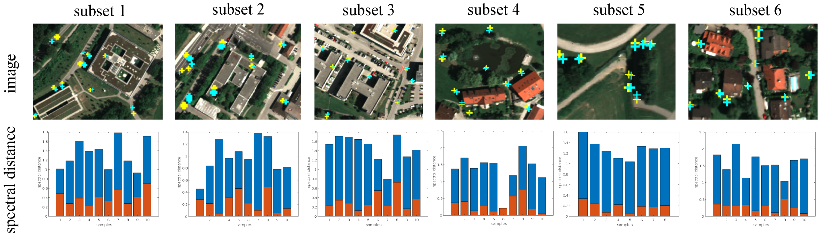
An important criteria of shadow restoration is the spectral distance between sunlit and shadowed pixels belonging to the same material. Ideally, the reflectance is an intrinsic property of materials, and should not change between sunlit and shadowed areas. Thus, the spectral distance between sunlit and shadowed pixels for one material in restored images should be significantly smaller than in the input images. In this paper, we compute the spectral distance using for the input images and for the restored images, respectively.
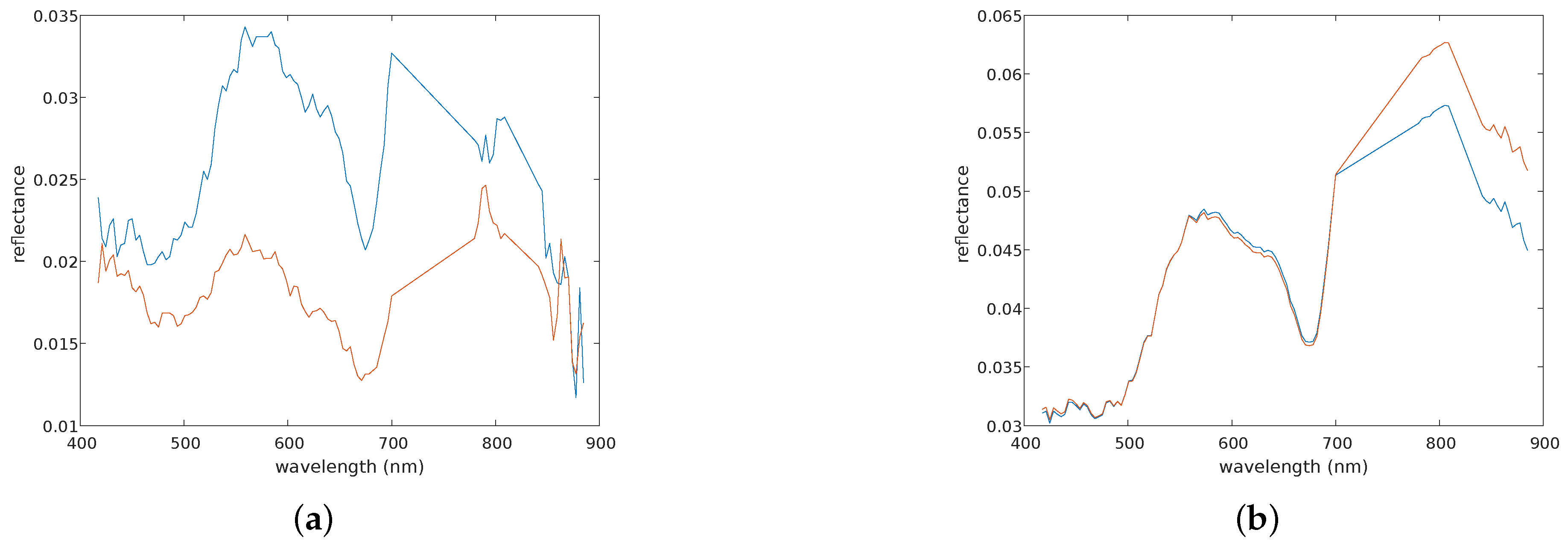
We select pairs of sun-shade pixels in each subset, as shown in the first row of Figure 5. For each pair of pixels, the yellow and cyan markers represent sunlit and shadowed pixels, respectively. Both markers in each pair are close to each other and to the shadow boundary, so we assume that the selected sunlit and shadowed pixels belong to the same material. The right column of Figure 5 shows the spectral distance between sunlit and shadowed pixels for each pair of pixels on the left column. The bars in blue and orange represent the spectral distances computed from the original and restored images, respectively. After shadow restoration, the spectral distances decrease significantly. One exception is represented by the sixth sample of subset 4, where the spectral distance increases by 0.1 after shadow restoration. This sample belongs to water, for which reflectances are small in both sunlit (lower than 0.035) and shadowed regions (lower than 0.025), as is shown in Figure 6. In addition, the shadowed water pixels are affected by nonlinear effects known to be relevant in water, and are shadowed also by trees. This causes the restored pixels to contain a small abundance value of the material “trees”, in the spectral range known as the red edge (Figure 6).
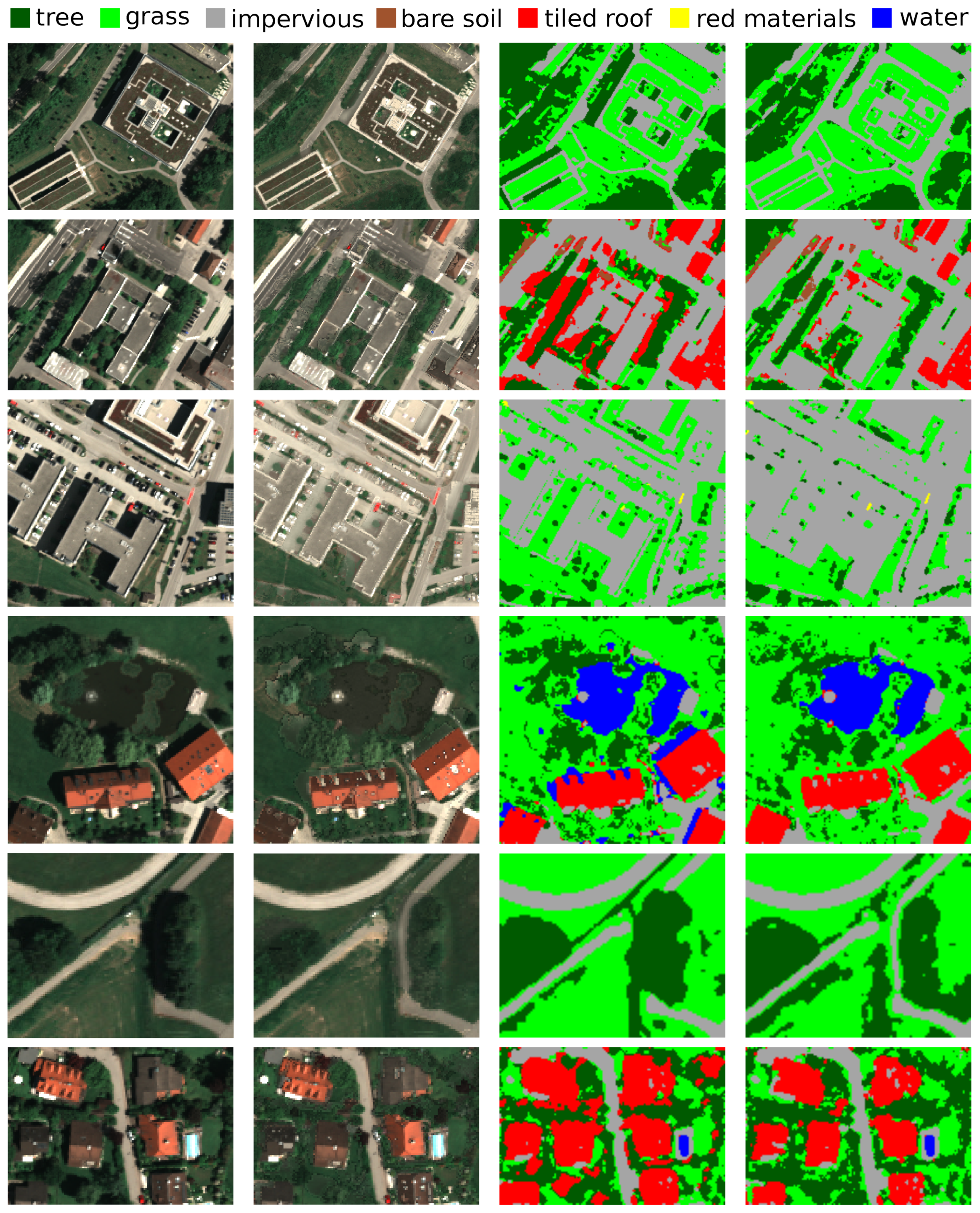
4.3. Restoration and Classification Results
Figure 7 compares input and restored images, along with their classifications. A total of 6565 training samples are manually selected from sunlit regions, while a total of 5927 test samples are selected in comparable quantities from both sunlit and shadowed regions. There are seven classes in six subsets, including tree, grass, impervious, bare soil, tiled roof, objects painted in red, i.e., red material, and water. As an example, Figure 8 reports a detailed comparison of pixel-wise classifications highlighting improvements after shadow restoration. The hyperspectral images used share the same acquisition and solar zenith angles. Therefore, we cannot validate our restored images with additional acquisitions with shadows occupying smaller areas. As an alternative, we compare the results with Google Earth images at same locations with the acquisition date of 10 July 2016 in Figure 9, with the assumption that most ground objects did not change within a two years time span.
The classifications of the input images are inaccurate for most of the shadowed regions. When the water class is not present in a subset, shadowed impervious surfaces are mostly classified as vegetation (1, 3, and 5) or tiled roof (subset 2). When water pixels are included in the training samples (subset 4), most of the shadowed regions are classified as water. The tree and grass pixels, both in input and restored images, are mostly classified as vegetation because the discriminative “red edge” feature typical of vegetation is visible also in shadowed areas. In addition to large and homogeneous areas, smaller objects are also recovered in shadowed regions. For example, subset 3 contains trees in the shadow, with tree crowns becoming visible in the restored image. A white car on the left side of the “H”-shape building in subset 3 is an example for other isolated objects being restored. Compared to white and red cars, dark objects, e.g., black cars, are considered as shadowed pixels in our proposed framework, as their reflectance values are small and comparable with shadowed pixels. In subset 3, these are restored as impervious surfaces.
Impervious surfaces shadowed by trees are sometimes classified as vegetation (e.g., on the top left side in subset 1). When pixels are shadowed by trees, especially in deep shadows, their spectra contain the “red edge” feature, due to incoming light interactions with the nearby trees. Thus, the abundance values of vegetation at these impervious surfaces are larger than zero, resulting in a mixture of impervious and vegetation materials in the reconstruction.
Table 2 presents the overall accuracies (OA) and Kappa (K) values of classification results. Both figures of merit increase by more than 10% in subsets 2, 4, 5, and 6, and increase by more than 20% in subsets 1 and 3. The increase in performance is due to the improved classification results in shadowed regions.
4.4. Sunlit Factor Map
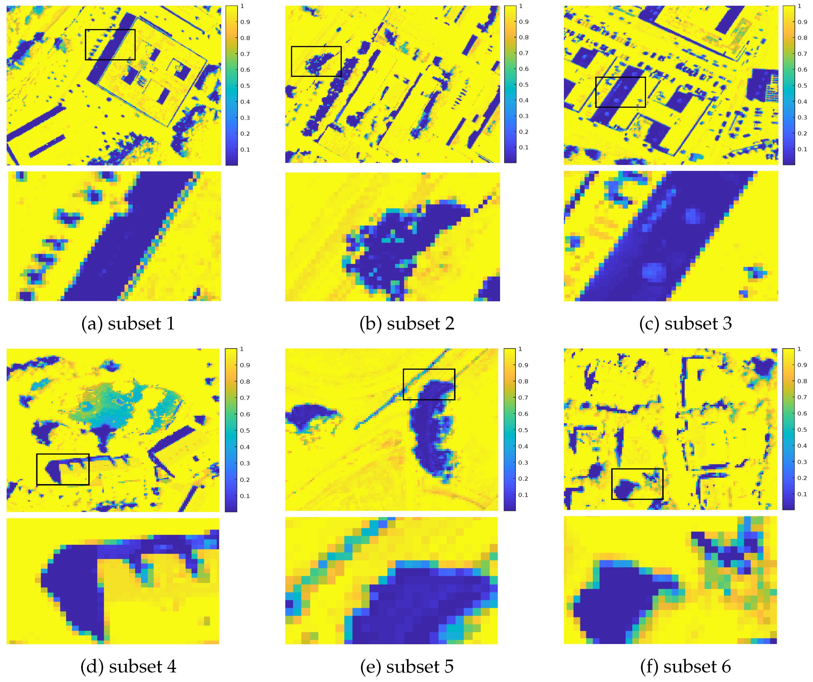
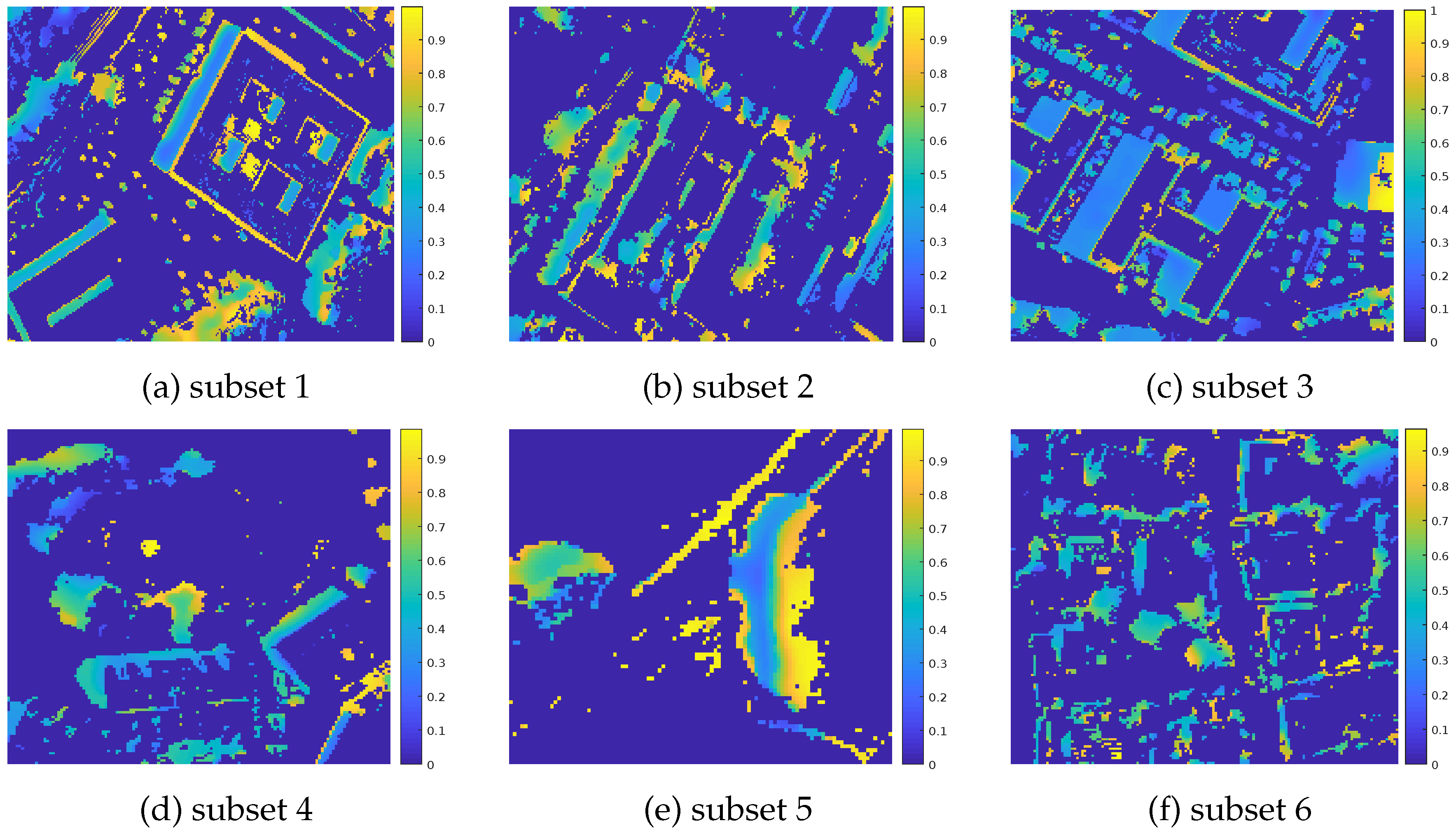
Sunlit factor maps in Figure 10 represent an additional output of the proposed framework. The values range from 0 to 1. Instead of a binary mask, Figure 10 shows a smooth transition between sunlit and shadowed areas, yielding a more realistic representation of shadows. In this paper, we set two thresholds and to identify pure shadowed pixels (value ) and pure sunlit pixels (value ). The values between and are regarded as transition areas between sunlit and shadowed pixels, i.e., shadow boundaries. When an area is shadowed by man-made objects, i.e., buildings, the transition areas are smaller. When an area is shadowed by vegetation, i.e., trees, the shadow boundaries span larger regions.
4.5. The F Parameter
For a pixel on the ground surface, the diffuse solar irradiance come isotropically from the sky [48]. For a given location and acquisition time, the proportion of diffuse to direct solar irradiance is constant. However, at a shadowed pixel where the sky is partially occluded, the diffuse solar irradiance decreases because the pixel can not see the sky from all directions. The F parameter (Figure 11) represents the scale of the proportion of diffuse to direct solar irradiance in Equation (5). We set F values at sunlit pixels to zeros, as F is relevant for the shadowed terms in Equation (8). The F values remain approximately homogeneous within one shadowed region and slightly increase on the shadow boundaries. Among different shadowed regions, pixels shadowed by vegetation show moderately larger values with respect to pixels shadowed by man-made objects.
5. Discussion
5.1. Level of Automatism
The framework runs automatically giving as input a hyperspectral image, the selected endmembers, and the relevant parameters. This implies that our method so far depends on manually selected endmembers, as the input spectral library is composed by pure pixels selected in sunlit regions exclusively. However, to the best of our knowledge, existing endmember extraction methods either do ignore shadowed regions, or regard shadowed regions as an additional dark endmember. Thus, the extracted endmembers usually contain pixels in shadowed regions or on the shadow boundaries, which cannot be used in our framework. In addition, the input spectral library should consider the fact that the observed values of the same material in hyperspectral images may vary, due to the spectral variability effect [56], which has been taken into account by manually selecting endmembers.
An endmember extraction method that excludes shadowed regions and shadow boundaries would not only help our specific framework, but also yield a more consistent physical representation of a scene, as the reflectance of a specific material should not change according to illumination conditions. Therefore, we introduce a simple but effective way of extracting endmembers automatically by taking into account shadows.
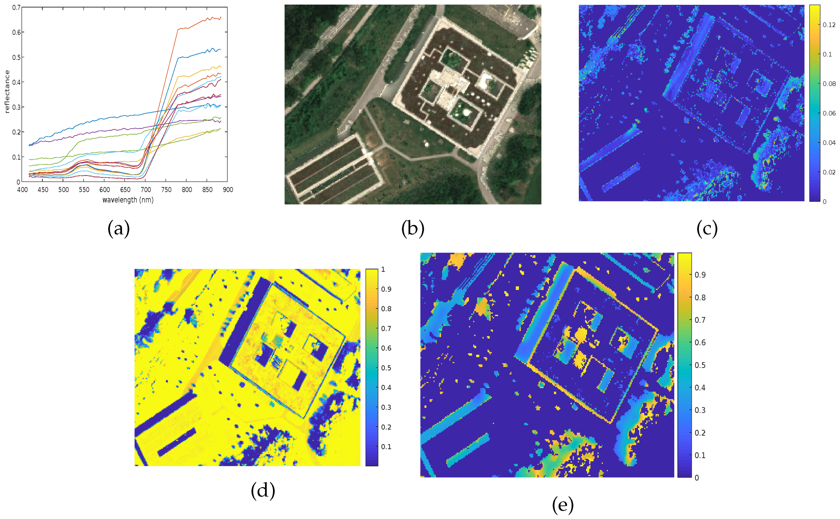
A straightforward way of selecting sunlit pixels is thresholding. In our experiment in subset 1, all the pixels having mean reflectance larger than an empirical threshold (set to 0.08 in this paper) are selected as candidate sunlit pixels. However, this may include some pixels located at shadow boundaries. Thus, a Canny edge detector [57] has been applied to detect and remove all boundary pixels from sunlit pixels candidates. In addition, considering the endmember variability effect, we apply the method in [58] to extract endmember bundles based on Vertex Component Analysis (VCA) [59]. By merging similar endmembers, we show the automatically extracted endmembers in Figure 12a. By using endmembers reported in Figure 12a and our proposed framework, our results are shown in Figure 12b,d,e. Both restoration and computed parameters are visually similar to the results obtained by employing the manually selected endmembers. Figure 12c depicts the Euclidean distance of the images of subset 1 restored by manual and automatic endmember extraction, having a maximum value of 0.13. This slight difference is due to the slightly different sets of endmembers selected.
5.2. Computational Cost
All algorithms were developed in MATLAB and run on an Intel Core i7 −8650 U CPU, 1.90 GHz machine with 4 Cores and 8 Logical Processors. We use the MATLAB function FMINCON to perform nonlinear optimization. The processing time depends on the number of input pixels and endmembers. If a shadow map is unknown, the algorithm requires 2445 s to restore the image subset number 1, having a size of pixels. Otherwise, the algorithm needs 1031 additional seconds to produce a sunlit factor map. On the other hand, if a shadow detection map is given, then the algorithm processes only shadowed pixels, requiring 948 s for shadow restoration.
5.3. Benefits and Challenges
The proposed framework shows promising results on detecting shadows and restoring spectral information in shadowed regions for hyperspectral imagery.
Methods proposed for shadow restoration in RGB and multispectral images are difficult to adapt to hyperspectral images, as their characteristics pose specific challenges [27,60]. For example, shadow removal methods may use ground images [44,60] as training and test data, which would not work in the case of airborne images. In addition, simple scenes are often used as test data [31], where a single shadowed region exists in one test image. This assumption often does not hold for airborne images containing more complicated scenarios. The proposed framework contributes to the open problems in the following aspects.
As a first aspect, some previous works assume diffuse solar irradiance to have zero [17] or constant values [32,34] across all wavelengths. These assumptions simplify real scenarios and may introduce errors in modeling shadowed spectra. The proposed framework considers diffuse irradiance and multiple reflections of direct solar irradiance as the illumination sources in shadowed regions, following physical assumptions. Second, several previous studies develop shadow detection and restoration methods in two separate frameworks, indicating that accurate shadow detection results are required to achieve satisfying restoration [30,42]. Our proposed framework computes shadow detection maps based on the residual analysis of pixel reconstruction through spectral unmixing, thus it does not require a shadow map as additional input. Third, a soft shadow detection yields a more realistic representation of shadows with respect to a binary shadow mas as, from a physical point of view, shadow boundaries are usually neither pure sunlit nor pure shadowed pixels. In addition, soft shadow masks allow some flexibility as they can be thresholded by an user to generate conservative or complete binary masks. Fourth, our framework does not require a large amount of training data, usually scarcely available and expensive to derive.
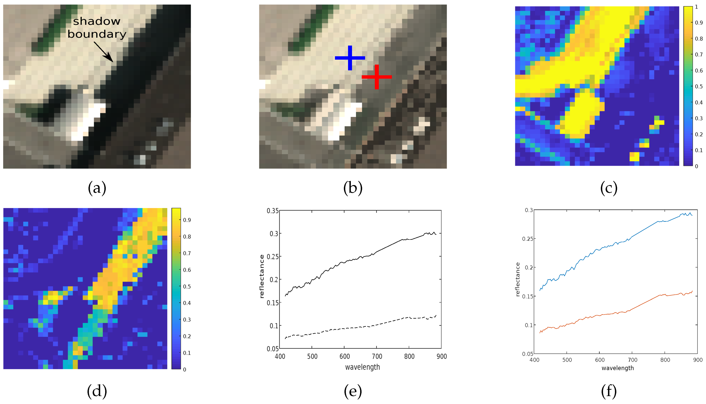
The proposed framework still contains several open problems. First, despite the correct classification results, we observe spectral distortions of shadowed pixels for some impervious surfaces, if slightly different materials are present in the scenes. An area in subset 2 (Figure 13) shows an impervious surface shadowed by a building. The relative spectra appear distorted with respect to the neighboring sunlit pixels belonging to the same material, as it is assumed that pixels on opposite edges of a shadow boundary usually exhibit similar reflectance spectra. Thus, we investigate the abundance maps of endmembers dominating the sunlit regions (in Figure 13c) and shadowed regions (in Figure 13d). In Figure 13e, we show the reflectances of the endmembers corresponding to Figure 13c as a solid line and Figure 13d as a dashed line, respectively. The spectral angle between the two reflectances in Figure 13e is equal to 0.035, indicating that the related two materials are highly similar. In addition, the spectral angle assumes a value of 0.032 between two reflectances in sunlit and shadowed pixels marked with a “+” in the restored image (Figure 13f). This implies that, when the spectral angle between two spectra is small, the restored results may not distinguish the related materials.
Second, endmembers used in the framework do not include black objects, such as cars in subset 3, because spectra of black objects are similar to shadowed pixels. Thus, the proposed framework regards black objects as shadows, as their sunlit factor values are low (Figure 10).
Third, although the sunlit factor values of water regions are higher with respect to shadowed pixels (Figure 10d), water can still be confused with shadows due do its low albedo. Thus, and for sunlit water pixels are comparable and considerably smaller than 0.1.
6. Conclusions
In this paper, motivated by the fact that reflectance values for a given material should be independent from illumination conditions, we have proposed a novel framework for shadow detection and restoration of hyperspectral images based on nonlinear unmixing. The framework regards pure sunlit and shadowed spectra as sunlit and shadowed endmembers, respectively. Pure sunlit spectra are manually selected from the input images, while pure shadowed spectra are computed from sunlit spectra based on physical assumptions. Subsequently, the algorithm solves abundances related to sunlit and shadowed endmembers through a nonlinear mixture model. Then, we reconstruct restored images pixel-wise using abundance maps and only the sunlit endmembers. As a byproduct, the proposed framework can generate sunlit factor maps that can locate sunlit pixels. Finally, sunlit pixels in the restored images are switched back to their original values. The proposed framework is tested on real airborne hyperspectral images both by visual analysis and quantitative assessments. Compared with two well-known mixture models, i.e., the linear mixture model (LMM) and the Fan model, our proposed mixture model can reconstruct shadowed pixels with significantly lower errors. After restoration, shadowed regions become visually alike to adjacent sunlit regions, and exhibit similar reflectance values. In addition, classification results are visually more convincing and accuracies increase by more than 10% for the investigated subsets after shadow restoration. The derived sunlit factor maps can produce soft shadow masks, representing natural transitions around shadow boundaries. We also demonstrate the possibility of detecting and including new materials in the input endmember library.
The work carried out so far raises open issues which are of interest for further investigation. Embedding spatial information may decrease the spectral distortion between highly similar materials in the neighborhood of shadow boundaries, where materials exhibit low variation in spectral shapes and large differences in absolute magnitude. In addition, black objects and water regions require further investigation. Future works could consider spectral bands that can increase the distinction between shadow and dark objects. Finally, the nonlinear mixture model in this paper allows the interactions of up to two endmembers. Higher-order nonlinear models could be included to model more accurately the physical interactions of the different light sources in the scene.
Author Contributions
The contributions of the individual authors are as follows: conceptualization, G.Z. and D.C.; methodology, G.Z. and D.C.; software, G.Z.; validation, G.Z. and D.C.; writing—original draft preparation, G.Z.; writing—review and editing, D.C., G.Z.; supervision, D.C. and R.M. All authors have read and agreed to the published version of the manuscript.
Funding
This research received no external funding.
Acknowledgments
The authors would like to thank Rudolf Richter for assistance with atmospheric correction of hyperspectral images.
Conflicts of Interest
The authors declare no conflict of interest.
References
- Shahtahmassebi, A.; Yang, N.; Wang, K.; Moore, N.; Shen, Z. Review of shadow detection and de-shadowing methods in remote sensing. Chin. Geogr. Sci. 2013, 23, 403–420. [Google Scholar] [CrossRef] [Green Version]
- Song, H.; Huang, B.; Zhang, K. Shadow detection and reconstruction in high-resolution satellite images via morphological filtering and example-based learning. IEEE Trans. Geosci. Remote Sens. 2013, 52, 2545–2554. [Google Scholar] [CrossRef]
- Dare, P.M. Shadow analysis in high-resolution satellite imagery of urban areas. Photogramm. Eng. Remote Sens. 2005, 71, 169–177. [Google Scholar] [CrossRef] [Green Version]
- Ashton, E.A.; Wemett, B.D.; Leathers, R.A.; Downes, T.V. A novel method for illumination suppression in hyperspectral images. In Algorithms and Technologies for Multispectral, Hyperspectral, and Ultraspectral Imagery XIV; International Society for Optics and Photonics: Orlando, FL, USA, 2008; Volume 6966, p. 69660C. [Google Scholar]
- Polder, G.; Gowen, A. The hype in spectral imaging. J. Spectr. Imaging 2020, 9. [Google Scholar] [CrossRef]
- Bioucas-Dias, J.M.; Plaza, A.; Camps-Valls, G.; Scheunders, P.; Nasrabadi, N.; Chanussot, J. Hyperspectral remote sensing data analysis and future challenges. IEEE Geosci. Remote Sens. Mag. 2013, 1, 6–36. [Google Scholar] [CrossRef] [Green Version]
- Adeline, K.R.; Chen, M.; Briottet, X.; Pang, S.; Paparoditis, N. Shadow detection in very high spatial resolution aerial images: A comparative study. ISPRS J. Photogramm. Remote Sens. 2013, 80, 21–38. [Google Scholar] [CrossRef]
- Nagao, M.; Matsuyama, T.; Ikeda, Y. Region extraction and shape analysis in aerial photographs. Comput. Graph. Image Process. 1979, 10, 195–223. [Google Scholar] [CrossRef]
- Rüfenacht, D.; Fredembach, C.; Süsstrunk, S. Automatic and accurate shadow detection using near-infrared information. IEEE Trans. Pattern Anal. Mach. Intell. 2013, 36, 1672–1678. [Google Scholar] [CrossRef]
- Qiao, X.; Yuan, D.; Li, H. Urban shadow detection and classification using hyperspectral image. J. Indian Soc. Remote Sens. 2017, 45, 945–952. [Google Scholar] [CrossRef]
- Tsai, V.J. A comparative study on shadow compensation of color aerial images in invariant color models. IEEE Trans. Geosci. Remote Sens. 2006, 44, 1661–1671. [Google Scholar] [CrossRef]
- Sarabandi, P.; Yamazaki, F.; Matsuoka, M.; Kiremidjian, A. Shadow detection and radiometric restoration in satellite high resolution images. In Proceedings of the 2004 IEEE International Geoscience and Remote Sensing Symposium, IGARSS 2004, Anchorage, AK, USA, 20–24 September 2004; Volume 6, pp. 3744–3747. [Google Scholar]
- Han, H.; Han, C.; Lan, T.; Huang, L.; Hu, C.; Xue, X. Automatic shadow detection for multispectral satellite remote sensing images in invariant color spaces. Appl. Sci. 2020, 10, 6467. [Google Scholar] [CrossRef]
- Nakajima, T.; Tao, G.; Yasuoka, Y. Simulated recovery of information in shadow areas on IKONOS image by combing ALS data. In Proceedings of the Asian conference on remote sensing (ACRS), Kathmandu, Nepal, 25–29 November 2002. [Google Scholar]
- Zhan, Q.; Shi, W.; Xiao, Y. Quantitative analysis of shadow effects in high-resolution images of urban areas. In Proceedings of the 3nd International Symposium on Remote Sensing and Data Fusion Over Urban Areas, Tempe, AZ, USA, 14–16 March 2005. [Google Scholar]
- Tolt, G.; Shimoni, M.; Ahlberg, J. A shadow detection method for remote sensing images using VHR hyperspectral and LIDAR data. In Proceedings of the 2011 IEEE international geoscience and remote sensing symposium, Vancouver, BC, Canada, 24–29 July 2011; pp. 4423–4426. [Google Scholar]
- Adler-Golden, S.M.; Matthew, M.W.; Anderson, G.P.; Felde, G.W.; Gardner, J.A. Algorithm for de-shadowing spectral imagery. In Imaging Spectrometry VIII; International Society for Optics and Photonics: Seattle, WA, USA, 2002; Volume 4816, pp. 203–210. [Google Scholar]
- Richter, R.; Müller, A. De-shadowing of satellite/airborne imagery. Int. J. Remote Sens. 2005, 26, 3137–3148. [Google Scholar] [CrossRef]
- Cameron, M.; Kumar, L. Diffuse skylight as a surrogate for shadow detection in high-resolution imagery acquired under clear sky conditions. Remote Sens. 2018, 10, 1185. [Google Scholar] [CrossRef] [Green Version]
- Levine, M.D.; Bhattacharyya, J. Removing shadows. Pattern Recognit. Lett. 2005, 26, 251–265. [Google Scholar] [CrossRef]
- Vicente, T.F.Y.; Hou, L.; Yu, C.P.; Hoai, M.; Samaras, D. Large-scale training of shadow detectors with noisily-annotated shadow examples. In European Conference on Computer Vision (ECCV); Springer: Amsterdam, The Netherlands, 2016; pp. 816–832. [Google Scholar]
- Nguyen, V.; Yago Vicente, T.F.; Zhao, M.; Hoai, M.; Samaras, D. Shadow detection with conditional generative adversarial networks. In Proceedings of the IEEE International Conference on Computer Vision, Venice, Italy, 22–29 October 2017; pp. 4510–4518. [Google Scholar]
- Finlayson, G.D.; Hordley, S.D.; Lu, C.; Drew, M.S. On the removal of shadows from images. IEEE Trans. Pattern Anal. Mach. Intell. 2005, 28, 59–68. [Google Scholar] [CrossRef]
- Zhang, Y.; Chen, G.; Vukomanovic, J.; Singh, K.K.; Liu, Y.; Holden, S.; Meentemeyer, R.K. Recurrent Shadow Attention Model (RSAM) for shadow removal in high-resolution urban land-cover mapping. Remote Sens. Environ. 2020, 247, 111945. [Google Scholar] [CrossRef]
- Finlayson, G.D.; Drew, M.S.; Lu, C. Entropy minimization for shadow removal. Int. J. Comput. Vis. 2009, 85, 35–57. [Google Scholar] [CrossRef] [Green Version]
- Arbel, E.; Hel-Or, H. Shadow removal using intensity surfaces and texture anchor points. IEEE Trans. Pattern Anal. Mach. Intell. 2010, 33, 1202–1216. [Google Scholar] [CrossRef]
- Lorenzi, L.; Melgani, F.; Mercier, G. A complete processing chain for shadow detection and reconstruction in VHR images. IEEE Trans. Geosci. Remote Sens. 2012, 50, 3440–3452. [Google Scholar] [CrossRef]
- Zhang, L.; Zhang, Q.; Xiao, C. Shadow remover: Image shadow removal based on illumination recovering optimization. IEEE Trans. Image Process. 2015, 24, 4623–4636. [Google Scholar] [CrossRef]
- Xiao, Y.; Tsougenis, E.; Tang, C.K. Shadow removal from single RGB-D images. In Proceedings of the IEEE Conference on Computer Vision and Pattern Recognition, Columbus, OH, USA, 23–28 June 2014; pp. 3011–3018. [Google Scholar]
- Khan, S.H.; Bennamoun, M.; Sohel, F.; Togneri, R. Automatic shadow detection and removal from a single image. IEEE Trans. Pattern Anal. Mach. Intell. 2015, 38, 431–446. [Google Scholar] [CrossRef] [PubMed] [Green Version]
- Qu, L.; Tian, J.; He, S.; Tang, Y.; Lau, R.W. Deshadownet: A multi-context embedding deep network for shadow removal. In Proceedings of the IEEE Conference on Computer Vision and Pattern Recognition, Honolulu, HI, USA, 21–26 July 2017; pp. 4067–4075. [Google Scholar]
- Kruse, F.A.; Lefkoff, A.; Boardman, J.; Heidebrecht, K.; Shapiro, A.; Barloon, P.; Goetz, A. The spectral image processing system (SIPS)-interactive visualization and analysis of imaging spectrometer data. In AIP Conference Proceedings; American Institute of Physics: Pasadena, CA, USA, 1993; Volume 283, pp. 192–201. [Google Scholar]
- Roussel, G.; Weber, C.; Ceamanos, X.; Briottet, X. A sun/shadow approach for the classification of hyperspectral data. In Proceedings of the 2016 8th Workshop on Hyperspectral Image and Signal Processing, Evolution in Remote Sensing (WHISPERS), Los Angeles, CA, USA, 21–24 August 2016; pp. 1–5. [Google Scholar]
- Windrim, L.; Ramakrishnan, R.; Melkumyan, A.; Murphy, R.J. A physics-based deep learning approach to shadow invariant representations of hyperspectral images. IEEE Trans. Image Process. 2017, 27, 665–677. [Google Scholar] [CrossRef] [PubMed]
- Windrim, L.; Melkumyan, A.; Murphy, R.; Chlingaryan, A.; Nieto, J. Unsupervised feature learning for illumination robustness. In Proceedings of the 2016 IEEE International Conference on Image Processing (ICIP), Phoenix, AZ, USA, 25–28 September 2016; pp. 4453–4457. [Google Scholar]
- Zhang, Q.; Pauca, V.P.; Plemmons, R.J.; Nikic, D.D. Detecting objects under shadows by fusion of hyperspectral and lidar data: A physical model approach. In Proceedings of the 2013 5th Workshop on Hyperspectral Image and Signal Processing, Evolution in Remote Sensing (WHISPERS), Gainesville, FL, USA, 25–28 June 2013; pp. 1–4. [Google Scholar]
- Friman, O.; Tolt, G.; Ahlberg, J. Illumination and shadow compensation of hyperspectral images using a digital surface model and non-linear least squares estimation. In Image and Signal Processing for Remote Sensing XVII; International Society for Optics and Photonics: Prague, Czech Republic, 2011; Volume 8180, p. 81800Q. [Google Scholar]
- Dobigeon, N.; Tourneret, J.Y.; Richard, C.; Bermudez, J.C.M.; McLaughlin, S.; Hero, A.O. Nonlinear unmixing of hyperspectral images: Models and algorithms. IEEE Signal Process. Mag. 2013, 31, 82–94. [Google Scholar] [CrossRef] [Green Version]
- Plaza, A.; Martínez, P.; Pérez, R.; Plaza, J. A quantitative and comparative analysis of endmember extraction algorithms from hyperspectral data. IEEE Trans. Geosci. Remote Sens. 2004, 42, 650–663. [Google Scholar] [CrossRef]
- Yang, J.; He, Y.; Caspersen, J. Fully constrained linear spectral unmixing based global shadow compensation for high resolution satellite imagery of urban areas. Int. J. Appl. Earth Obs. Geoinf. 2015, 38, 88–98. [Google Scholar] [CrossRef]
- Nascimento, J.M.; Bioucas-Dias, J.M. Nonlinear mixture model for hyperspectral unmixing. In Image and Signal Processing for Remote Sensing XV; International Society for Optics and Photonics: Berlin, Germany, 2009; Volume 7477, p. 74770I. [Google Scholar]
- Omruuzun, F.; Baskurt, D.O.; Daglayan, H.; Cetin, Y.Y. Shadow removal from VNIR hyperspectral remote sensing imagery with endmember signature analysis. In Next-Generation Spectroscopic Technologies VIII; International Society for Optics and Photonics: Baltimore, MD, USA, 2015; Volume 9482, p. 94821F. [Google Scholar]
- Heylen, R.; Scheunders, P. A multilinear mixing model for nonlinear spectral unmixing. IEEE Trans. Geosci. Remote Sens. 2015, 54, 240–251. [Google Scholar] [CrossRef]
- Guo, R.; Dai, Q.; Hoiem, D. Single-image shadow detection and removal using paired regions. In CVPR 2011; IEEE: Providence, RI, USA, 2011; pp. 2033–2040. [Google Scholar]
- Mo, N.; Zhu, R.; Yan, L.; Zhao, Z. Deshadowing of urban airborne imagery based on object-oriented automatic shadow detection and regional matching compensation. IEEE J. Sel. Top. Appl. Earth Obs. Remote Sens. 2018, 11, 585–605. [Google Scholar] [CrossRef]
- Zhang, G.; Cerra, D.; Mueller, R. Towards the Spectral Restoration of Shadowed Areas in Hyperspectral Images Based on Nonlinear Unmixing. In Proceedings of the 2019 10th Workshop on Hyperspectral Imaging and Signal Processing, Evolution in Remote Sensing (WHISPERS), Amsterdam, The Netherlands, 24–26 September 2019; pp. 1–5. [Google Scholar]
- Zhang, G.; Cerra, D.; Mueller, R. Improving the classification in shadowed areas using nonlinear spectral unmixing. In Proceedings of the 2020 IEEE International Geoscience and Remote Sensing Symposium (IGARSS), Waikoloa Village, HI, USA, 16–26 July 2020. in press. [Google Scholar]
- Schott, J.R. Remote Sensing: The Image Chain Approach; Oxford University Press on Demand: New York, NY, USA, 2007. [Google Scholar]
- Heylen, R.; Parente, M.; Gader, P. A review of nonlinear hyperspectral unmixing methods. IEEE J. Sel. Top. Appl. Earth Obs. Remote Sens. 2014, 7, 1844–1868. [Google Scholar] [CrossRef]
- Fan, W.; Hu, B.; Miller, J.; Li, M. Comparative study between a new nonlinear model and common linear model for analysing laboratory simulated-forest hyperspectral data. Int. J. Remote Sens. 2009, 30, 2951–2962. [Google Scholar] [CrossRef]
- Slater, P.N.; Doyle, F.; Fritz, N.; Welch, R. Photographic systems for remote sensing. Man. Remote Sens. 1983, 1, 231–291. [Google Scholar]
- Bredies, K.; Kunisch, K.; Pock, T. Total generalized variation. SIAM J. Imaging Sci. 2010, 3, 492–526. [Google Scholar] [CrossRef]
- Köhler, C.H. Airborne imaging spectrometer hyspex. J. Large Scale Res. Facil. JLSRF 2016, 2, 1–6. [Google Scholar] [CrossRef] [Green Version]
- Richter, R.; Schläpfer, D.; Müller, A. An automatic atmospheric correction algorithm for visible/NIR imagery. Int. J. Remote Sens. 2006, 27, 2077–2085. [Google Scholar] [CrossRef]
- Keshava, N.; Mustard, J.F. Spectral unmixing. IEEE Signal Process. Mag. 2002, 19, 44–57. [Google Scholar] [CrossRef]
- Borsoi, R.A.; Imbiriba, T.; Bermudez, J.C.M.; Richard, C.; Chanussot, J.; Drumetz, L.; Tourneret, J.Y.; Zare, A.; Jutten, C. Spectral Variability in Hyperspectral Data Unmixing: A Comprehensive Review. arXiv 2020, arXiv:2001.07307. [Google Scholar]
- Canny, J. A computational approach to edge detection. IEEE Trans. Pattern Anal. Mach. Intell. 1986, 6, 679–698. [Google Scholar] [CrossRef]
- Somers, B.; Zortea, M.; Plaza, A.; Asner, G.P. Automated extraction of image-based endmember bundles for improved spectral unmixing. IEEE J. Sel. Top. Appl. Earth Obs. Remote Sens. 2012, 5, 396–408. [Google Scholar] [CrossRef] [Green Version]
- Nascimento, J.M.; Dias, J.M. Vertex component analysis: A fast algorithm to unmix hyperspectral data. IEEE Trans. Geosci. Remote Sens. 2005, 43, 898–910. [Google Scholar] [CrossRef] [Green Version]
- Cun, X.; Pun, C.M.; Shi, C. Towards Ghost-Free Shadow Removal via Dual Hierarchical Aggregation Network and Shadow Matting GAN. In Proceedings of the AAAI, New York, NY, USA, 7–12 February 2020; pp. 10680–10687. [Google Scholar]
Figure 1.
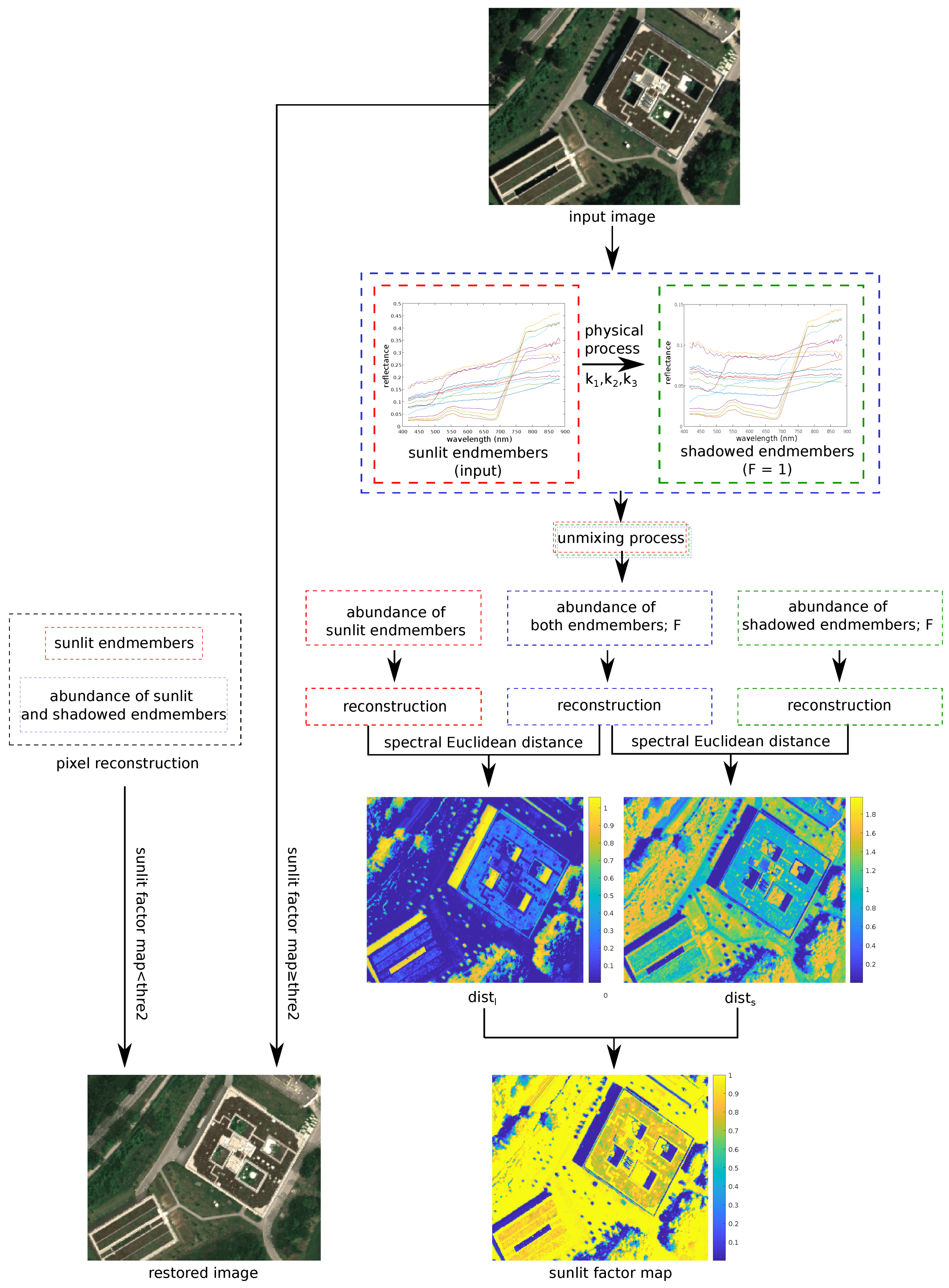
The proposed framework. The inputs are a hyperspectral image, the physical parameters , , and , and a spectral library containing manually selected endmembers in sunlit regions, i.e., sunlit endmembers. After the unmixing process, the restored image is reconstructed by a nonlinear combination of the sunlit endmembers, using the abundances of the same materials in the shadow. The framework outputs the sunlit factor map, computed by spectral Euclidean distances of the reconstruction results. Finally, in order to avoid introducing spectral distortions, sunlit pixels in the restored image are switched back to their original values.
Figure 1.
The proposed framework. The inputs are a hyperspectral image, the physical parameters , , and , and a spectral library containing manually selected endmembers in sunlit regions, i.e., sunlit endmembers. After the unmixing process, the restored image is reconstructed by a nonlinear combination of the sunlit endmembers, using the abundances of the same materials in the shadow. The framework outputs the sunlit factor map, computed by spectral Euclidean distances of the reconstruction results. Finally, in order to avoid introducing spectral distortions, sunlit pixels in the restored image are switched back to their original values.

Figure 2.
An example of selecting pure sunlit (with blue marker) and shadowed pixels (with red marker) for the same material.
Figure 2.
An example of selecting pure sunlit (with blue marker) and shadowed pixels (with red marker) for the same material.

Figure 3.
Six subsets selected from scenes acquired with similar acquisition conditions in the study area of Oberpfaffenhofen, Bavaria, Germany.
Figure 3.
Six subsets selected from scenes acquired with similar acquisition conditions in the study area of Oberpfaffenhofen, Bavaria, Germany.

Figure 4.
Six subsets with manually selected sunlit endmembers.

Figure 5.
Comparison of spectral Euclidean distance between input and restored images. First column: the six subsets considered. Second column: spectral distance of up to 10 pairs of samples in each subset (input and restored images in blue and orange, respectively).
Figure 5.
Comparison of spectral Euclidean distance between input and restored images. First column: the six subsets considered. Second column: spectral distance of up to 10 pairs of samples in each subset (input and restored images in blue and orange, respectively).

Figure 6.
Mean reflectance of water regions in subset 4 of Figure 5. The blue and red color represents mean reflectance of sunlit and shadowed pixels, respectively. Pixels are selected from (a) the input image and (b) the restored image for subset 4.
Figure 6.
Mean reflectance of water regions in subset 4 of Figure 5. The blue and red color represents mean reflectance of sunlit and shadowed pixels, respectively. Pixels are selected from (a) the input image and (b) the restored image for subset 4.

Figure 7.
Rows: Six subsets. First column: input images; second column: restored images; third column: classification maps of the input images; last column: classification maps of the restored images.
Figure 7.
Rows: Six subsets. First column: input images; second column: restored images; third column: classification maps of the input images; last column: classification maps of the restored images.

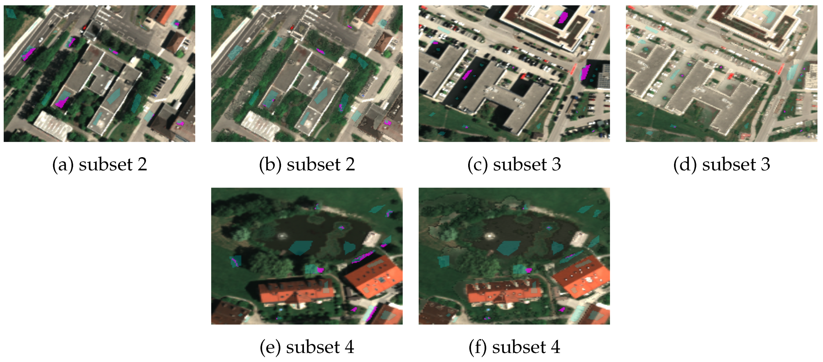
Figure 8.
Comparison of classification results in Table 2 for input images (a,c,e) and restored images (b,d,f) in subsets 2, 3, and 4. Correctly and incorrectly classified areas are marked in cyan and magenta, respectively.
Figure 8.
Comparison of classification results in Table 2 for input images (a,c,e) and restored images (b,d,f) in subsets 2, 3, and 4. Correctly and incorrectly classified areas are marked in cyan and magenta, respectively.

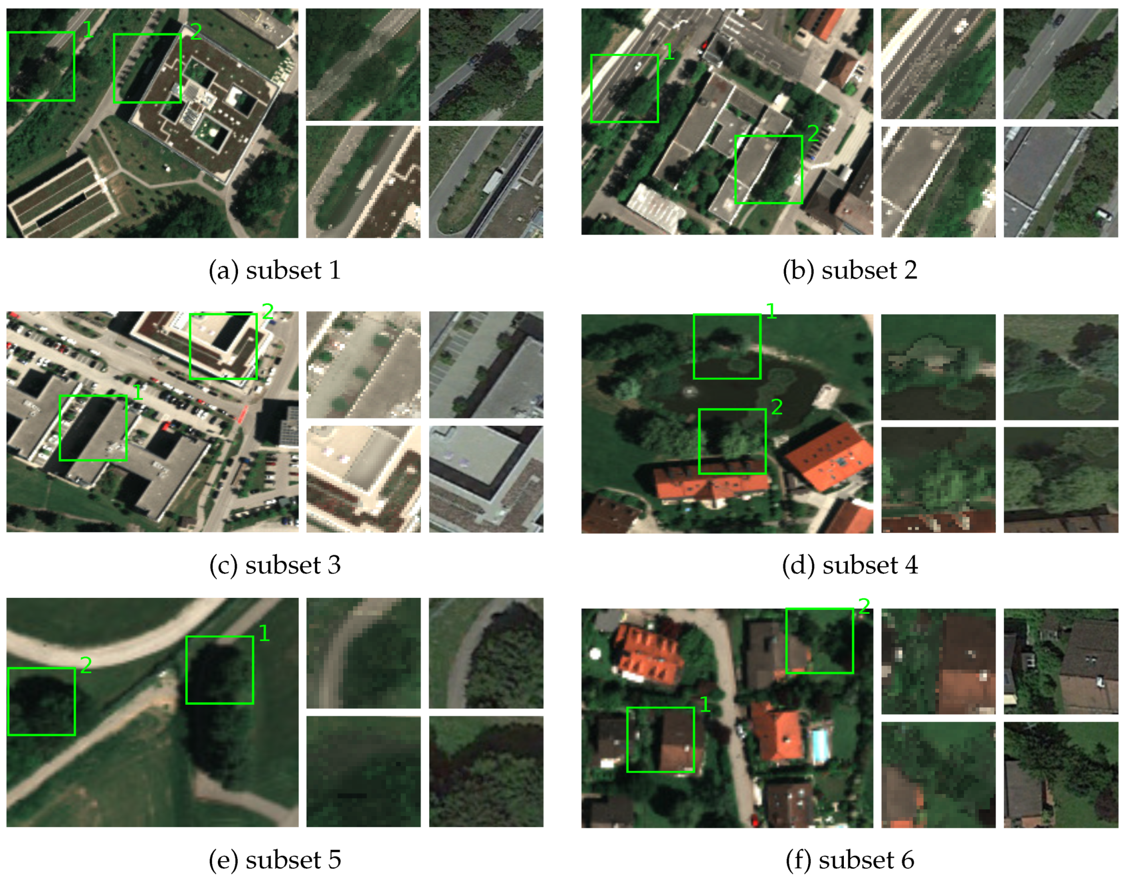
Figure 9.
Comparison between restored subsets and Google Earth images. For each subset, on the left: input image with two selected regions of interest; rows on the right: regions of interest from the restored image and screenshots from Google Earth data in which shadowed areas are partially sunlit.
Figure 9.
Comparison between restored subsets and Google Earth images. For each subset, on the left: input image with two selected regions of interest; rows on the right: regions of interest from the restored image and screenshots from Google Earth data in which shadowed areas are partially sunlit.

Figure 10.
Sunlit factor maps ranging from 0 to 1. Values smaller than are considered as pure shadowed pixels. Values larger than are regarded as pure sunlit pixels. For each subset, top: sunlit factor map marked with the region of interest; bottom: zoomed-in image of the region of interest.
Figure 10.
Sunlit factor maps ranging from 0 to 1. Values smaller than are considered as pure shadowed pixels. Values larger than are regarded as pure sunlit pixels. For each subset, top: sunlit factor map marked with the region of interest; bottom: zoomed-in image of the region of interest.

Figure 11.
The F parameter with the range of values from 0 to 1.

Figure 12.
Shadow detection and restoration using automatically extracted endmembers in subset 1. (a) Extracted endmembers; (b) restored image; (c) Euclidean distance between restored images using manually and automatically extracted endmembers; (d) sunlit factor map; (e) F parameter.
Figure 12.
Shadow detection and restoration using automatically extracted endmembers in subset 1. (a) Extracted endmembers; (b) restored image; (c) Euclidean distance between restored images using manually and automatically extracted endmembers; (d) sunlit factor map; (e) F parameter.

Figure 13.
An example of spectral inconsistency in the neighborhood of a shadow boundary. Subset images from (a) the input image of subset 2 and (b) the restored image of subset 2; (c) abundance map for a material dominating the sunlit region; (d) abundance map for a material dominating the shadowed region; (e) endmembers corresponding to the abundance maps of (c) as a solid line and (d) as a dashed line; (f) reflectance of sunlit (blue) and shadowed (red) pixels in (b).


Table 1.
Mean reconstruction errors for six subsets.
| Subset | Region | LMM | FAN | Proposed |
|---|---|---|---|---|
| 1 | sunlit regions | 0.113 | 0.083 | 0.077 |
| shadowed regions | 0.414 | 0.421 | 0.026 | |
| both | 0.191 | 0.171 | 0.064 | |
| 2 | sunlit regions | 0.088 | 0.077 | 0.071 |
| shadowed regions | 0.209 | 0.210 | 0.021 | |
| both | 0.114 | 0.106 | 0.060 | |
| 3 | sunlit regions | 0.092 | 0.090 | 0.081 |
| shadowed regions | 0.708 | 0.738 | 0.023 | |
| both | 0.290 | 0.298 | 0.062 | |
| 4 | sunlit regions | 0.059 | 0.044 | 0.039 |
| shadowed regions | 0.099 | 0.100 | 0.018 | |
| both | 0.064 | 0.052 | 0.037 | |
| 5 | sunlit regions | 0.088 | 0.079 | 0.063 |
| shadowed regions | 0.0685 | 0.732 | 0.030 | |
| both | 0.199 | 0.200 | 0.057 | |
| 6 | sunlit regions | 0.126 | 0.108 | 0.117 |
| shadowed regions | 0.156 | 0.158 | 0.025 | |
| both | 0.132 | 0.118 | 0.084 |
Table 2.
Comparison of classification accuracies using input and restored images.
| Data | Input | Restored |
|---|---|---|
| subset 1 | OA = 73.472% K = 0.552 | OA = 95.366% K = 0.927 |
| subset 2 | OA = 82.203% K = 0.715 | OA = 93.553% K = 0.883 |
| subset 3 | OA = 55.0% K = 0.366 | OA = 93.939% K = 0.880 |
| subset 4 | OA = 84.495% K = 0.799 | OA = 95.138% K = 0.937 |
| subset 5 | OA = 80.340% K = 0.703 | OA = 90.170% K = 0.852 |
| subset 6 | OA = 85.373% K = 0.80 | OA = 93.284% K = 0.908 |
Publisher’s Note: MDPI stays neutral with regard to jurisdictional claims in published maps and institutional affiliations. |
© 2020 by the authors. Licensee MDPI, Basel, Switzerland. This article is an open access article distributed under the terms and conditions of the Creative Commons Attribution (CC BY) license (http://creativecommons.org/licenses/by/4.0/).
Share and Cite
MDPI and ACS Style
Zhang, G.; Cerra, D.; Müller, R. Shadow Detection and Restoration for Hyperspectral Images Based on Nonlinear Spectral Unmixing. Remote Sens. 2020, 12, 3985. https://0-doi-org.brum.beds.ac.uk/10.3390/rs12233985
AMA Style
Zhang G, Cerra D, Müller R. Shadow Detection and Restoration for Hyperspectral Images Based on Nonlinear Spectral Unmixing. Remote Sensing. 2020; 12(23):3985. https://0-doi-org.brum.beds.ac.uk/10.3390/rs12233985
Chicago/Turabian StyleZhang, Guichen, Daniele Cerra, and Rupert Müller. 2020. "Shadow Detection and Restoration for Hyperspectral Images Based on Nonlinear Spectral Unmixing" Remote Sensing 12, no. 23: 3985. https://0-doi-org.brum.beds.ac.uk/10.3390/rs12233985
Note that from the first issue of 2016, this journal uses article numbers instead of page numbers. See further details here.