Monitoring Hybrid Rice Phenology at Initial Heading Stage Based on Low-Altitude Remote Sensing Data

Abstract

Accurate monitoring of hybrid rice phenology (RP) is crucial for breeding rice cultivars and controlling fertilizing amount. The aim of this study is to monitor the exact date of hybrid rice initial heading stage (IHS_DAS) based on low-altitude remote sensing data and analyze the influence factors of RP. In this study, six field experiments were conducted in Ezhou city and Lingshui city from 2016 to 2019, which involved different rice cultivars and nitrogen rates. Three low-altitude remote sensing platforms were used to collect rice canopy reflectance. Firstly, we compared the performance of normalized difference vegetation index (NDVI) and red edge chlorophyll index (CIred edge) for monitoring RP. Secondly, double logistic function (DLF), asymmetric gauss function (AGF), and symmetric gauss function (SGF) were used to fit time-series CIred edge for acquiring phenological curves (PC), the feature: maximum curvature (MC) of PC was extracted to monitor IHS_DAS. Finally, we analyzed the influence of rice cultivars, N rates, and air temperature on RP. The results indicated that CIred edge was more appropriate than NDVI for monitoring RP without saturation problem. Compared with DLF and AGF, SGF could fit CIred edge without over fitting problem. MC of SGF_CIred edge from all three platforms showed good performance in monitoring IHS_DAS with good robustness, R² varied between 0.82 and 0.95, RMSE ranged from 2.31 to 3.81. In addition, the results demonstrated that high air temperature might cause a decrease of IHS_DAS, and the growth process of rice was delayed when more nitrogen fertilizer was applied before IHS_DAS. This study illustrated that low-altitude remote sensing technology could be used for monitoring field-scale hybrid rice IHS_DAS accurately.

1. Introduction

With the rapid growth of the world population, food security has become an urgent issue, attracting worldwide attention. Rice is a very important crop that provides staple food for almost 50% of the world’s population [1]. Hybrid vigor (heterosis) is a universal phenomenon in crops, and the yield of hybrid rice is usually higher than that of conventional rice [2,3]. Hybrid rice makes a great contribution to the world’s food security, with more than half the growth of rice yield [4,5,6]. Hybrid rice is widely planted in large areas of Asian region, including China, Japan, and Southeast Asian countries. Breeding hybrid rice cultivars with high yield and good quality has been an important part of these countries’ strategies for developing modernized agriculture [7].

Rice phenology (RP) is critical for farm management and yield evaluation [8]. RP is divided into germination, seeding, tillering, jointing, booting, heading and flowering, grain filling, and milk stages [9]. Breeding hybrid rice is a time-consuming and laborious physical work. It is difficult for breeders to walk in the rice fields, which are fragmented by roads and water networks [10]. The heading and flowering stage is the essential time for breeders to choose superior parents and execute pollination operation. In general, when hybrid rice is at heading and flowering stage, flowers bloom daily between 9:00 am to 2:00 pm lasting 7–12 days [11,12,13], which means that breeders should finish a series of breeding operations accurately and timely, such as selecting appropriate rice spike, pollination, bagging, and labeling. Moreover, the flowering habit of rice is closely related to rice yield [14]. Thus, monitoring field-scale rice initial heading stage (IHS) accurately is not only important for breeding hybrid rice, but also for rice yield estimation [15].

To date, there are three main methods for monitoring vegetation phenology: ground observation [16], vegetation growth models [17] and remote sensing estimation [18]. Traditionally, ground observation is a time-consuming and laborious work, including sampling, visual observation, taking photos and writing reports, which is suitable to acquire accurate in situ phenology information in small areas [19]. Rice growth models (e.g., CERES-Rice, ORYZA2000, RCM, Beta Model, and SIMRIW) can precisely simulate the growth process of rice [20], but these models consist of many parameters (e.g., rainfall, illumination, air temperature, vegetation cultivars, fertilization and irrigation) that are complicated for monitoring region scale vegetation phenology [21,22,23]. Compared with the aforementioned two methods, many studies have proved that remote sensing is a time-saving and cost-effective method for monitoring vegetation phenology at both local and regional scales, avoiding sampling bias and strenuous labor [24,25,26,27,28,29].

At present, RP is mainly monitored by optical satellites and Synthetic Aperture Radar (SAR) satellites on large scale. Optical satellites have shorter revisiting cycle and lower cost [30]. A variety of vegetation indices (VIs) from optical satellites are widely used to monitor vegetation growth and phenology [31,32]. Sakamoto et al. [33] adopted wavelet and Fourier transforms to filter the time-series enhanced vegetation index (EVI) from moderate resolution imaging spectroradiometer (MODIS) images for monitoring rice planting date, heading date and harvesting date. The root mean square errors (RMSE) of the estimated phenological dates against the statistical data were 12.1 days, 9.0 days and 10.6 days, respectively. Onojeghuo et al. [34] fused MODIS data with Landsat data for acquiring the high spatiotemporal data (30 m spatial resolution and 8-day intervals), and proved that normalized difference vegetation index (NDVI) extracted from the fused data could improve the accuracy of RP. Sun et al. [35] proposed the red edge chlorophyll index (CIred edge) from Sentinel-2 images to evaluate cadmium stress in rice at different stages. However, the optical satellites were affected by atmospheric disturbances, solar radiation and cloud cover [36,37]. The estimation error of phenology could be as high as nine days or even more. SAR satellites have the advantage to work at all-weather situation and all-day, and are very sensitive to vegetation morphological structure information [38,39]. Some studies demonstrated that the backscattering information of SAR had good relationship with RP on large scale. Fikriyah et al. [40] discriminated the transplanted rice and direct seeded rice by temporal Sentinel-1 SAR. TerraSAR-X was applied to monitor RP on Biologische Bundesanstalt, Bundessortenamt und CHemische Industrie (BBCH) scale [41,42]. He et al. [43] used the backscattering characteristics of multi-temporal RADARSAT-2 datasets to monitor the four rice phenological phases (transplanting, vegetative, reproductive and maturity), the overall accuracy (OA) is 86.2%. Although these studies indicated that optical satellites and SAR satellites could monitor large-scale RP successfully, it is still difficult to acquire precise field-scale RP due to the lack of high spatiotemporal satellite data.

Compared with satellites, low-altitude (below 500 m) remote sensing sensors have obvious advantages: less atmospheric interference, short visiting cycle, high spatial resolution and low cost. Low-altitude sensors, such as unmanned aerial vehicles (UAV) [44], fixed towers [45], and hand-held sensors [46], are gradually applied to monitor field-scale vegetation phenology [47]. Yang et al. [48] adopted a deep learning approach to detect RP based on UAV images, with an accuracy rate of 83.9% and mean absolute error (MAE) of 0.18. Bai et al. [49] utilized the fixed towers mounted with RGB cameras to achieve rice heading stage automatic observation. Lin et al. [50] calculated NDVI from a hand-held radiometer to monitor RP, the results showed that the maximum NDVI had a good correlation ship with the heading and flowering stage. Han et al. [51] proposed a deep convolutional neural network (DCNN) approach to analyze hand-held RGB images for real-time RP detection, with a high overall accuracy of 0.913 and low mean absolute error of 0.090. In addition, Zheng et al. [9] compared the ability of two ground-based spectral instruments for monitoring RP, there were 2.3–9.3 days difference between the observed date and estimated date at different growth stages. In a word, these studies proved that low-altitude remote sensing sensors had good performance in monitoring field-scale RP.

To our knowledge, there are three key steps to monitor vegetation phenology based on remote sensing technology: (1) cleaning and flagging remote sensing data; (2) reconstructing vegetation phenological curves; (3) extracting features for monitoring vegetation phenology [52]. However, previous studies mainly focused on studying the phenological characteristics of rice and exploring appropriate methods for monitoring RP. Few studies compared the advantages and disadvantages of different low-altitude remote sensing sensors for field-scale RP detection, and analyzed the influence factors of RP. Thus, the aim of this study is to (1) analyze the change regularity of typical time-series VIs (NDVI and CIred edge) during the whole growth stage of hybrid rice; (2) evaluate the performance of three functions for reconstructing rice phenological curves based on three low-altitude remote sensing data, and extract features of VIs for monitoring IHS_DAS; (3) analyze the influential factors (rice cultivars, N rates, and air temperature) of RP.

2. Materials and Methods

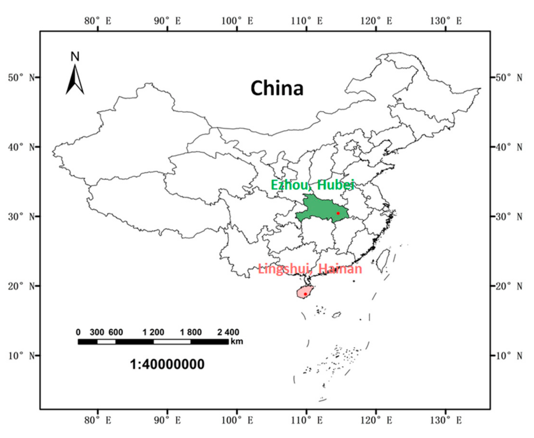
2.1. Experimental Sites

Six hybrid rice (Oryza sativa L. subsp. indica) experiments were conducted in this study (Figure 1). Experiments 1, 2, 5, and 6 were conducted in Ezhou city (30.3752°N, 114.7450°E), Hubei province, central China from May to October in 2016, 2017, 2018 and 2019. Ezhou city is located in a subtropical monsoon climate. The experiment 3 and 4 were conducted in Lingshui city (18.5302°N, 110.0545°E), Hainan province, southern China from December 2017 to May 2018. Lingshui city is located in a tropical marine monsoon climate.

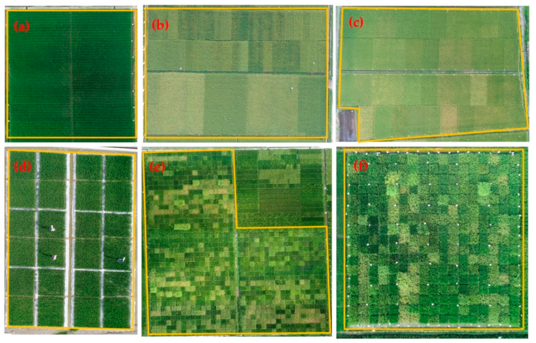
2.2. Experimental Design

Experiments 1, 2, and 3 were conducted in three growing seasons spanning from 2016 to 2018. Rice seeds were sown in seedling beds. 30 days after sowing (DAS), seedlings were transplanted into rice field with a unified density 225,000 plants/hm². The plot area of each rice cultivar was 40 m² (5.0 m × 8.0 m). For all treatments, N fertilizer (180 kg/hm²) was applied in the form of urea: 50% as basal fertilizer before transplanting, 25% at the tillering stage and 25% at the booting stage. Monocalcium phosphate (P₂O₅ 90 kg/hm²) and potassium chloride (K₂O 180 kg/hm²) were applied before transplanting. Other management decisions (pest control and herbicide application) followed the local standard practices.

Experiment 4 was a randomized complete block design with three replications for each treatment, involving two rice cultivars and four N rates. Rice cultivars were Fengliangyou 4 (FLY4) and Luoyou 9348 (LY9348). Four N rates: 0 (N0), 120 (N1), 180 (N2) and 240 (N3) kg/hm² were applied in the form of urea: 50% as basal fertilizer before transplanting, 50% at the booting stage. The 24 individual plot area was 15 m² (5.0 m × 3.0 m), respectively. In addition, other factors were the same with experiments 1, 2, and 3.

Experiment 5 and 6 were conducted from May to October of 2018 and 2019, involving 1014 and 289 rice cultivars, each rice cultivar was planted in an individual plot, and the area of plot was 1 m² (1.0 m × 1.0 m), respectively. In addition, other factors were the same with experiments 1, 2, and 3.

Six experiments involved different hybrid rice cultivars and N rates, as detailed in Figure 2 and

Table 1. Details of six experiments.

Experiment	Year and Study Site	Number of Plots	Plots Area (m2)	Sowing Time (Month/Day/Year)	Number of Rice Cultivars	N Rates (kg/hm2)
1	2016 Ezhou	16	40	5/7/2016	16	180
2	2017 Ezhou	52	40	5/7/2017	52	180
3	2017–2018 Lingshui	40	40	12/10/2017	40	180
4	2017–2018 Lingshui	24	15	12/10/2017	2	0, 120, 180 and 240
5	2018 Ezhou	1014	1	5/25/2018	1014	180
6	2019 Ezhou	289	1	5/15/2019	289	180

.

2.3. Experimental Data

2.3.1. Meteorological Data

Meteorological data were collected from the China Meteorological Data Service Center (http://www.weather.com.cn/), which included maximum air temperature (T_max), minimum air temperature (T_min) and weather conditions spanning from 2016 to 2019. In order to show weather conditions clearly, we used different numbers to represent different weather conditions: 1 represented sunny, 2 represented cloudy, 3 represented overcast, 4 represented shower, 5 represented light rain, 6 represented moderate rain, 7 represented heavy rain, and 8 represented rainstorm, respectively.

2.3.2. Field Phenological Data

In our study, the phenological time was recorded as days after sowing (DAS). Ground field observations and records were carried out according to the specifications for agrometeorological observation-Rice (http://www.cma.gov.cn/root7/auto13139/201903/t20190329_519169.html) from the China Meteorological Administration. For example, when 10% of investigated rice grew spikes, the exact date was defined as the time of rice phenology at initial heading stage (IHS_DAS). Then, we investigated 40 hills of rice plants in experiments 1, 2, 3, and 4, and 20 hills of rice plants in experiments 5 and 6 were investigated by random method, respectively.

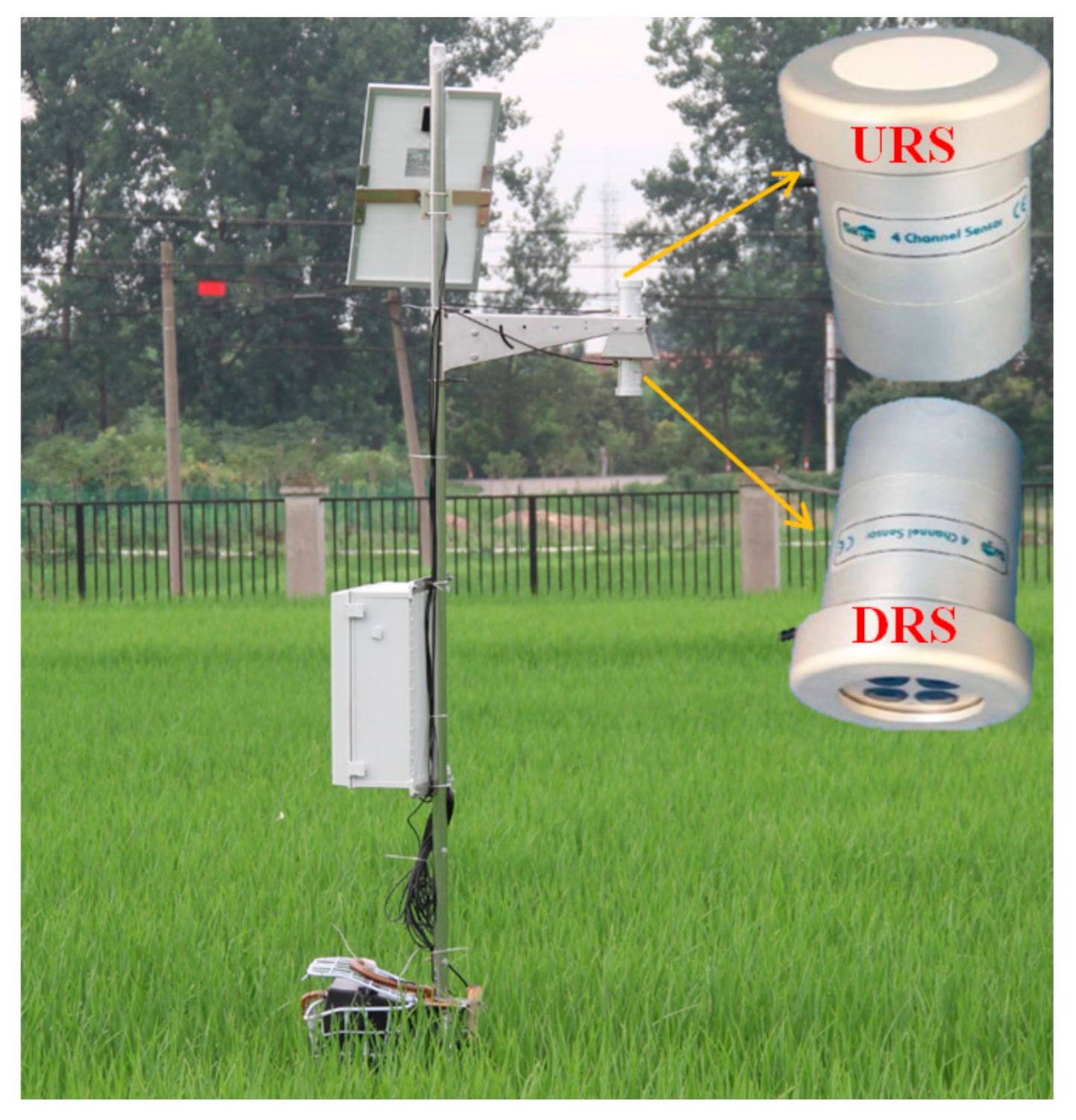
2.3.3. Daily Reflectance

Three sets of SKYE radiometers (SKR 1860, SKYE Instruments Ltd., Llandrindod Wells, UK) were employed to collect four bands reflectance every 30 min. In order to distinguish SKYE radiometers, we marked them as A_SKYE, B_SKYE and C_SKYE. Each set of SKYE radiometers consisted of two sensors: the upward radiometer sensor (URS) and the downward radiometer sensor (DRS). URS measured downwelling (DW) radiance with the aid of a cosine corrector, which collected radiance from sky in 180° hemisphere above the sensor. DRS measured the 25° field of view upwelling (UW) radiance from rice canopy. During the whole growth stage of rice, all SKYE radiometers were positioned above rice canopy at a height of 2 m with a 25° field-of-view of 0.62 m² area (Figure 3). The specifications of SKYE radiometers are listed in

Table 2. The specifications of SKYE radiometers.

SKYE Radiometers	URS		DRS
	Central Wavelength (nm)	Band Width (nm)	Central Wavelength (nm)	Band Width (nm)
A_SKYE	550.3	39.9	549.7	39.8
	655.1	34.6	655.3	34.7
	717.2	23.7	716.8	23.6
	865.6	28.5	865.0	31.5
B_SKYE	550.0	39.9	549.9	38.7
	655.1	36.7	654.9	36.0
	716.6	23.6	717.7	23.9
	865.3	27.9	865.7	29.7
C_SKYE	551.8	39.6	549.5	39.7
	652.9	35.7	653.4	35.9
	717.0	26.2	715.8	25.2
	857.4	38.0	858.3	37.8

.

SKYE radiometric calibration: the relative reflectance of four bands could be calculated using the following equation.

$$\begin{gathered} R_{\lambda }=\frac{U{W}_{\lambda }}{D{W}_{\lambda }}\times \mathsf{\pi } \\ \left(\lambda =550, 655, 717 \mathrm{and} 865 \mathrm{nm}\right) \end{gathered}$$

(1)

where $U{W}_{\lambda }$ and $D{W}_{\lambda }$ are calculated (mol m⁻² s⁻¹), respectively.

In four growing seasons spanning from 2016 to 2019, SKYE radiometers collected continuously reflectance of three rice cultivars: LY 9348, FLY 4, and Yi Liang You Hua Zhan (YLYHZ), as detailed in

Table 3. Details of SKYE measurements.

Experiment	Year and Study Site	SKYE Radiometers	Rice Cultivars	IHSDAS	N Rates (kg/hm2)
1	2016 Ezhou	C_SKYE	LY 9348	97	180
2	2017 Ezhou	A_SKYE	FLY 4	85	180
		B_SKYE	YLYHZ	77	180
		C_SKYE	LY 9348	87	180
4	2017–2018 Lingshui	A_SKYE	LY 9348	106	120
		B_SKYE	FLY 4	109	120
		C_SKYE	LY 9348	109	240
6	2019 Ezhou	A_SKYE	FLY 4	89	180
		B_SKYE	LY 9348	91	180

. The median reflectance between 10:00 am to 2:00 pm was calculated as daily reflectance to reduce the impact of weather drastic change.

2.3.4. The Hyperspectral Reflectance

The hyper-spectrometer ASD Field Spec 4 (ASD Inc., Boulder, CO, USA) was employed to collect rice canopy reflectance in experiment 1, 2, 3 and 4, with the spectrum ranging from 350–2500 nm. The measurements were conducted on sunny days from 10:00 am to 2:00 pm. A white reference panel (Chemical composition: BaSO₄, Size: 25.4 × 25.4 cm) was used to make relative radiometric correction before each measurement. The optical fiber probe of ASD was positioned above rice canopy at a height of 1 m with a 25° field-of-view of 0.15 m² area. Five fixed points’ spectral measurements were averaged to reduce uncertainty error of spectral measurement in each plot. The hyperspectral reflectance involved different rice cultivars, as detailed in

Table 4. Details of ASD measurements.

Experiment	Year and Study Site	Measurement Dates (Month/Day/Year)	Days after Sowing (DAS)	Number of Rice Cultivars
1	2016 Ezhou	7/28/2016	82	16
		8/11/2016	96	16
		9/2/2016	118	16
		9/21/2016	137	16
2	2017 Ezhou	6/20/2017	44	52
		7/7/2017	61	52
		7/18/2017	72	52
		8/6/2017	91	52
		8/23/2017	108	52
		9/12/2017	128	52
3	2017–2018 Lingshui	2/4/2018	56	40
		2/25/2018	77	40
		3/9/2018	89	40
		3/19/2018	99	40
		3/31/2018	111	40
		4/28/2018	138	40
4	2017–2018 Lingshui	2/4/2018	56	24
		2/22/2018	74	24
		3/4/2018	84	24
		3/14/2018	94	24
		3/24/2018	104	24
		4/4/2018	115	24
		4/29/2018	140	24

.

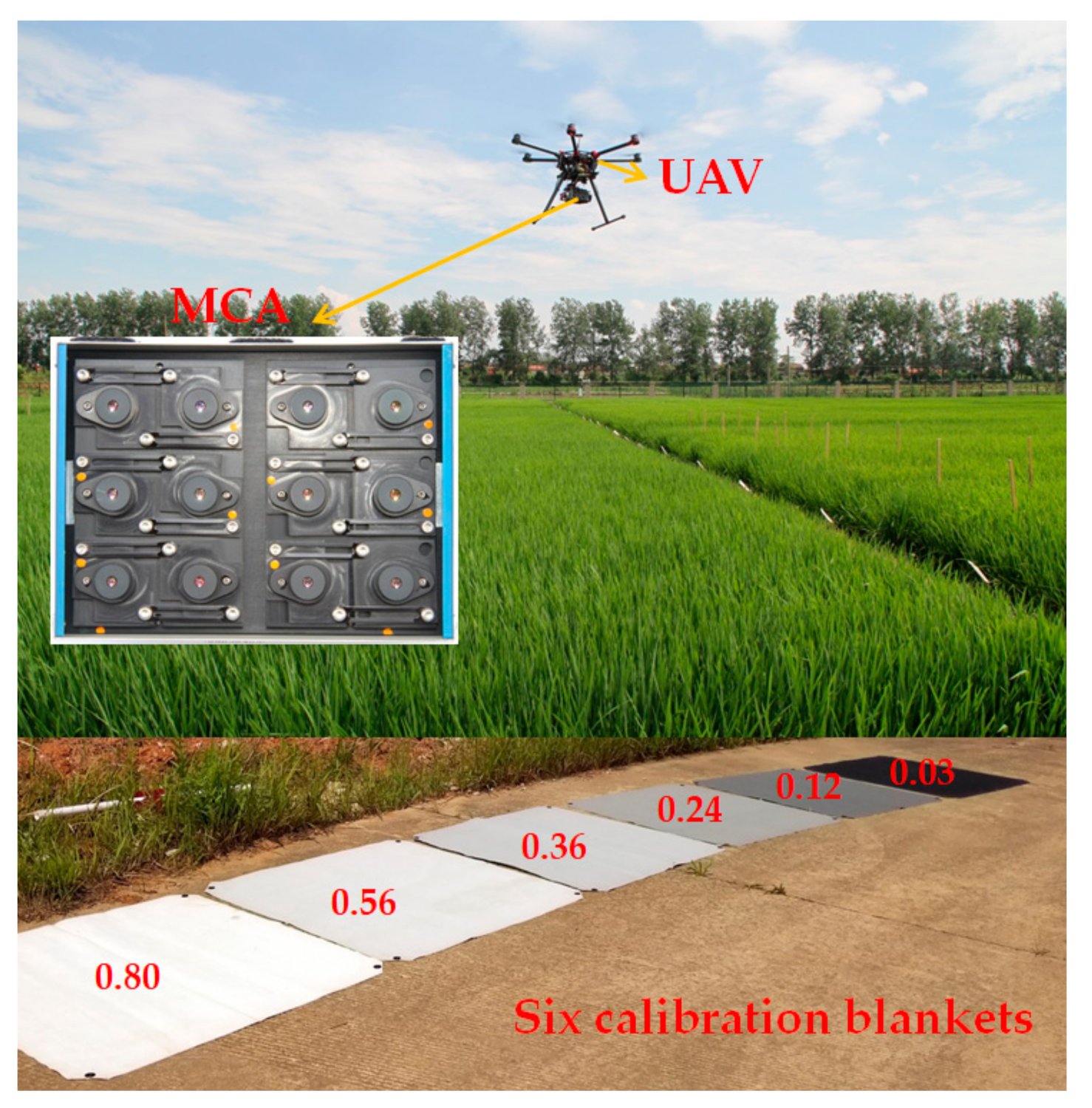
2.3.5. The UAV Multispectral Reflectance

In this study, a multispectral camera (MCA, Tetracam Inc., Chatsworth, CA, USA) was mounted on an eight-propeller UAV (S1000, DJI Technology Co., Ltd., Shenzhen, China) to acquire the panoramic multispectral images in experiment 5 and 6. The UAV flight was conducted on sunny days between 10:00 am to 2:00 pm. The flight duration varied between 10 and 15 min. The flight height was 120 m with a field of view 83.25 m × 66.50 m, with the ground sampling distance 6.5 cm/pixel.

MCA consisted of twelve individual digital miniature cameras equipped with different band pass filters centered at the wavelength of 490 nm, 520 nm, 550 nm, 570 nm, 670 nm, 680 nm, 700 nm, 720 nm, 800 nm, 850 nm, 900 nm, and 950 nm respectively (

Table 5. Center wavelength and bandwidth of MCA.

Band Number	Center Wavelength (nm)	Bandwidth (nm)	Band Number	Center Wavelength (nm)	Bandwidth (nm)
1	490	10	7	700	10
2	520	10	8	720	10
3	550	10	9	800	10
4	570	10	10	850	10
5	670	10	11	900	20
6	680	10	12	950	40

). The multispectral images are recorded as digital number (DN) values. Prior to the flight, six calibration blankets were placed on the flat road as radiometric calibration targets (Figure 4). One panoramic multispectral image could simultaneously contain the six calibration blankets and the total field plots within the field of view of MCA. The calibration blankets were made with highly durable woven polyester fabric at the size of 1.2 m × 1.2 m, having the relatively constant reflectance of 0.03, 0.12, 0.24, 0.36, 0.56, and 0.80, respectively. As a linear relationship was assumed between surface reflectance and at-sensor radiance, the empirical line method (ELM) was used to convert DN to surface reflectance [53,54]. $Gai{n}_{\mathrm{k}}$ and $offse{t}_{\mathrm{k}}$ were calculated using the least-square method from the relatively constant reflectance (0.03, 0.12, 0.24, 0.36, 0.56, and 0.80) and the corresponding DN values of calibration targets. Then $Gai{n}_{\mathrm{k}}$ and $offse{t}_{\mathrm{k}}$ were applied to calculate the canopy surface of each pixel in multispectral images. The specific equations are as follows.

$$\left(\begin{array}{c}0.03\\ 0.12\\ 0.24\\ 0.36\\ 0.56\\ 0.80\end{array}\right)=\left(\begin{array}{c}D{N}_{\left(1,\mathrm{k}\right)}\\ D{N}_{\left(2,\mathrm{k}\right)}\\ D{N}_{\left(3,\mathrm{k}\right)}\\ D{N}_{\left(4,\mathrm{k}\right)}\\ D{N}_{\left(5,\mathrm{k}\right)}\\ D{N}_{\left(6,\mathrm{k}\right)}\end{array}\right)\times Gai{n}_{\mathrm{k}}+offse{t}_{\mathrm{k}}$$

(2)

$$\begin{gathered} R_{\mathrm{k}}=D{N}_{\mathrm{k}}\times Gai{n}_{\mathrm{k}}+offse{t}_k \\ \left(k=490, 520, 550, 570, 670, 680, 700, 720, 800, 850, 900 \mathrm{and} 950 \mathrm{nm}\right) \end{gathered}$$

(3)

where k is the center wavelengths of 12 bands, DN(i,k) are the digital number values of the calibration target i (i = 1, 2, 3, 4, 5, 6, respectively) in band k. $Gai{n}_{\mathrm{k}}$ and $offse{t}_{\mathrm{k}}$ represent the slope and intercept. $R_{\mathrm{k}}$ and $D{N}_{\mathrm{k}}$ are the canopy surface reflectance and the digital number values of multispectral images.

The UAV system collected multispectral images from May to October of 2018 and 2019, involving 1303 rice cultivars in total (

Table 6. Details of MCA measurements.

Experiment	Year and Study Site	Measurement Dates (Month/Day/Year)	Days after Sowing (DAS)	Number of Rice Cultivars
5	2018 Ezhou	6/27/2018	33	1014
		7/6/2018	42	1014
		7/11/2018	47	1014
		7/16/2018	52	1014
		7/27/2018	63	1014
		8/2/2018	69	1014
		8/9/2018	76	1014
		8/15/2018	82	1014
		8/21/2018	88	1014
		8/27/2018	94	1014
6	2019 Ezhou	2/7/2019	42	289
		6/7/2019	48	289
		14/7/2019	52	289
		22/7/2019	60	289
		27/7/2019	68	289
		1/8/2019	73	289
		6/8/2019	78	289
		11/8/2019	83	289
		16/8/2019	88	289
		22/8/2019	93	289
		29/8/2019	99	289
		3/9/2019	106	289
		9/9/2019	111	289
		17/9/2019	117	289

). PixelWrench2 software (Tetracam Inc., Chatsworth, CA, USA) was used to perform images preprocessing, including noise correction, vignetting correction, lens distortion correction, band-to-band registration and band stacking [55,56]. The radiometric calibration and reflectance extraction processing were performed using the ENVI software (Exelis Visual Information Solutions, Boulder, CO, USA).

After image preprocessing, we selected a region of interest (ROI) in the multispectral image, which included 100 pixels of 0.42 m² area in each plot. The plot-level reflectance was calculated as the average reflectance of all pixels within ROI.

2.4. Research Methods

2.4.1. Vegetation Indices (VIs)

Vegetation indices (VIs) refer to the spectral reflectance transformations of two or more bands, which are related to vegetation photosynthesis and nutrition status [57]. NDVI is the most commonly used VIs for quantitative remote sensing [58]. CIred edge has good performance in the estimation of chlorophyll content, leaf area index and biomass [59]. In this study, NDVI and CIred edge are employed to monitor RP. They are calculated as:

$$NDVI=({\rho }_{NIR}-{\rho }_{Red})/({\rho }_{NIR}+{\rho }_{Red})$$

(4)

$$CIred edge=({\rho }_{NIR}/{\rho }_{Red edge})-1$$

(5)

where ${\rho }_{NIR}$ is the reflectance in the wavelength of 865 nm in SKYE (800 nm in ASD and MCA), ${\rho }_{Red edge}$ is the reflectance in the wavelength of 717 nm in SKYE (720 nm in ASD and MCA), ${\rho }_{Red}$ is the reflectance in the wavelength of 655 nm in SKYE (680 nm in ASD and MCA).

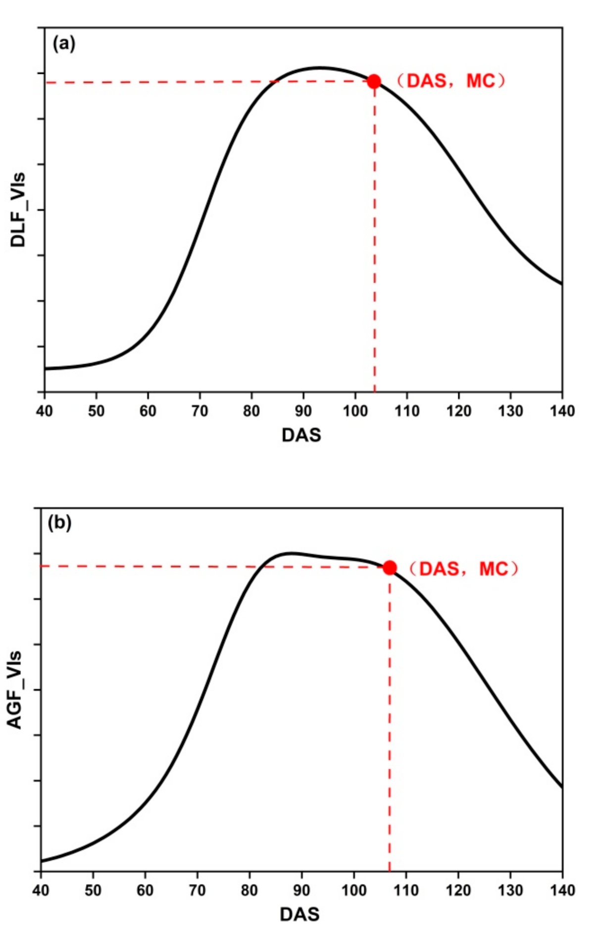
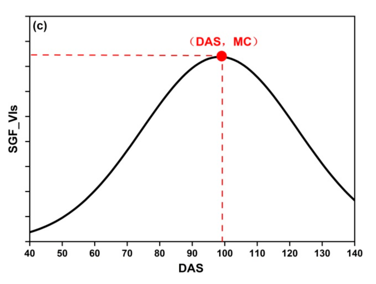
2.4.2. Fitting Functions

There were several methods to smooth and fit time-series VIs curves, such as dynamic threshold approach [60], derivative method [61], savitzky-golay smooth [62], double logistic function (DLF) [25], asymmetric gauss function (AGF) [63] and symmetric gauss function (SGF) [64]. Previous studies reported that DLF and AGF had good performance in fitting time-series VIs for monitoring vegetation phenology [65,66,67,68,69]. In our study, to obtain high quality time-series VIs, three fitting functions (DLF, AGF, and SGF) were applied to fit time-series VIs for reconstructing three phenological curves (PC): DLF_VIs, AGF_VIs, and SGF_VIs. The feature: the maximum curvature (MC) of PC was extracted to monitor IHS_DAS.

The calculation formulas are as follows:

$$\mathrm{DLF}\_\mathrm{VIs}=\frac{c}{\left(1+e^{\left(a+b\ast DAS\right)}\right)}+\frac{g}{\left(1+e^{\left(d+f\ast DAS\right)}\right)}$$

(6)

$$\mathrm{AGF}\_\mathrm{VIs}=h{e}^{-{\left(\frac{DAS-i}{j}\right)}^2}+k{e}^{-{\left(\frac{DAS-l}{m}\right)}^2}$$

(7)

$$\mathrm{SGF}\_\mathrm{VIs}=p{e}^{-{\left(\frac{DAS-q}{r}\right)}^2}$$

(8)

where $DAS$ are the days after rice sowing, corresponding the time of VIs acquisition, $e$ is the natural constant, a, b, c, d, f, g, h, i, j, k, l, m, p, q, and r are the best parameters of three fitting functions (DLF, AGF, and SGF), respectively.

$$\mathrm{MC}=\max (\frac{\left|P{C}^{″}\right|}{{(1+{(P{C}^{\prime })}^2)}^{\frac{3}{2}}})$$

(9)

where PC are the phenological curves: DLF_VIs, AGF_VIs, and SGF_VIs, PC′ is the first derivative of PC, and PC″ is the second derivative of PC. MC is the maximum curvature of PC (Figure 5).

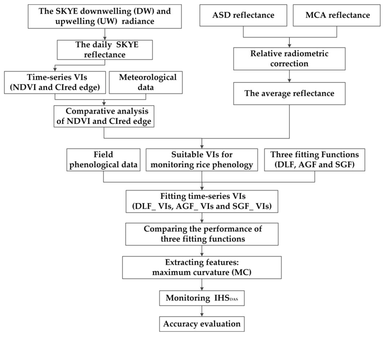
2.4.3. The Process of Modeling

Figure 6 shows the flowchart. Firstly, we calculated the reflectance of different remote sensing platforms. The statistical analysis of meteorological data and field phenological data were carried out. Secondly, daily NDVI and CIred edge were computed using the SKYE reflectance. We analyzed the phenological change of rice during the whole growth stage, and compared the characteristics of NDVI and CIred edge for monitoring RP. Thirdly, the VIs (NDVI or CIred edge) were computed using the reflectance of ASD and MCA. Three fitting functions (DLF, AGF and SGF) were applied to fit the suitable VIs for reconstructing PC: DLF_VIs, AGF_Vis, and SGF_VIs. We evaluated the performance of three fitting functions. Finally, we extracted the MC of PC for monitoring IHS_DAS and evaluated the accuracy.

2.4.4. The Assessment of Models

The coefficient of determination (R²) and root mean square error (RMSE) were used to evaluate the performances of three fitting functions and the accuracy of monitoring IHS_DAS. Mathematically, a higher R² and smaller RMSE represent better model accuracy.

$${\mathrm{R}}^2=1-\frac{{\sum }_{i=1}^n{\left(y_i-x_i\right)}^2}{{\sum }_{i=1}^n{\left(y_i-\overline{y}\right)}^2}$$

(10)

$$\mathrm{RMSE}=\sqrt{\frac{{\sum }_{i=1}^n{\left(y_i-x_i\right)}^2}{n}}$$

(11)

where $x_i$ and $y_i$ are the estimated and measured values, $\overline{y}$ is the average of the measured values, and n is the sample number, respectively.

The mathematical models were performed using MATLAB R2018a (MathWorks, Inc., Natick, MA, USA). Graphics were prepared using Origin 9.1 software program (OriginLab Corporation, Northampton, MA, USA).

3. Results

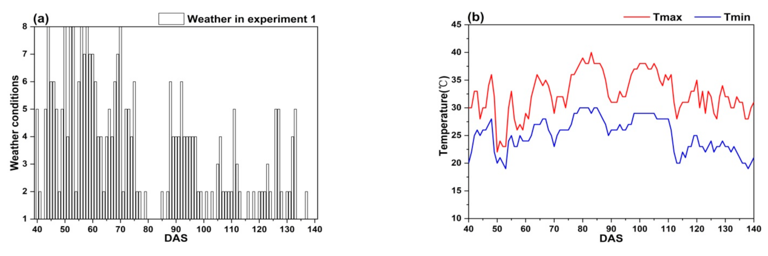
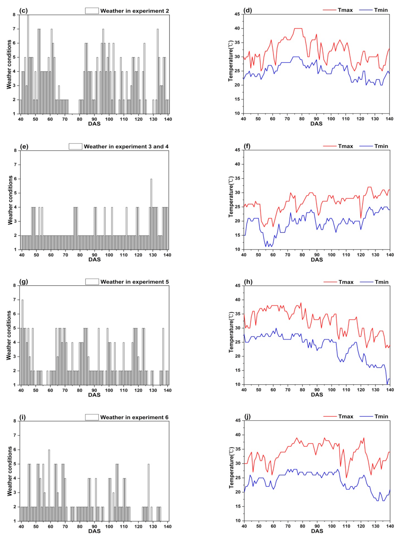
3.1. Statistical Analysis of Meteorological Data

Figure 7 shows that the weather conditions have obvious difference between two climatic zones, the climate of Lingshui city is more stable than that of Ezhou city.

In Ezhou city, the weather conditions in experiment 1 and 2 fluctuate greatly. It often rains during the whole growth period of rice (Figure 7a,c). Sometimes, there is even a regional heavy rain or rainstorm. Further, the continuous high temperature (T_max ≥ 35 °C) appears between DAS 76 to 88 and DAS 64 to 82 (Figure 7b,d). The weather conditions in experiment 5 and 6 are mainly sunny to cloudy with light rain occasionally (Figure 7g,i), however, the continuous high temperature (T_max ≥ 35 °C) appears between DAS 49 to 79 and DAS 70 to 105 (Figure 7h,j).

In Lingshui city, the weather conditions in experiments 3 and 4 are very stable. It is mainly sunny to cloudy with small air temperature change (Figure 7,f), there is not continuous high air temperature appearing during the whole growth period of rice. Good weather conditions in Lingshui city are helpful to obtain accurate remote sensing data.

3.2. Statistical Analysis of IHS_DAS

We carried out statistical analysis of IHS_DAS in six experiments (

Table 7. The statistical characteristics of IHS_DAS.

Experiment	Number of Plots	Minimum	Mean	Maximum	Standard Deviation	Variance	Coefficient of Variation (%)
1	16	92	98.31	104	3.45	11.96	3.51
2	52	76	84.00	94	5.59	31.29	6.66
3	40	96	110.60	119	3.71	13.73	3.35
4	24	103	106.58	110	2.15	4.60	2.01
5	1014	59	76.38	103	7.44	55.40	9.74
6	289	60	87.42	122	9.27	85.84	10.60

). The mean values of IHS_DAS are 98.31, 84.00, 110.60, 76.38, and 87.42 in experiment 1, 2, 3, 5 and 6, while the coefficients of variation are 3.51%, 6.66%, 3.35%, 9.74%, and 10.60%. IHS_DAS ranges from 59 to 122 in six experiments. The statistical indicators of IHS_DAS show the significant differences in IHS_DAS among different rice cultivars. The maximum and minimum value of IHS_DAS in experiment 4 are 103 and 110 involving four N rates, it implies that N rates have obvious effects on IHS_DAS. Therefore, we take into account rice cultivars and nitrogen treatments in this study and focus on building robust and accurate models for monitoring IHS_DAS.

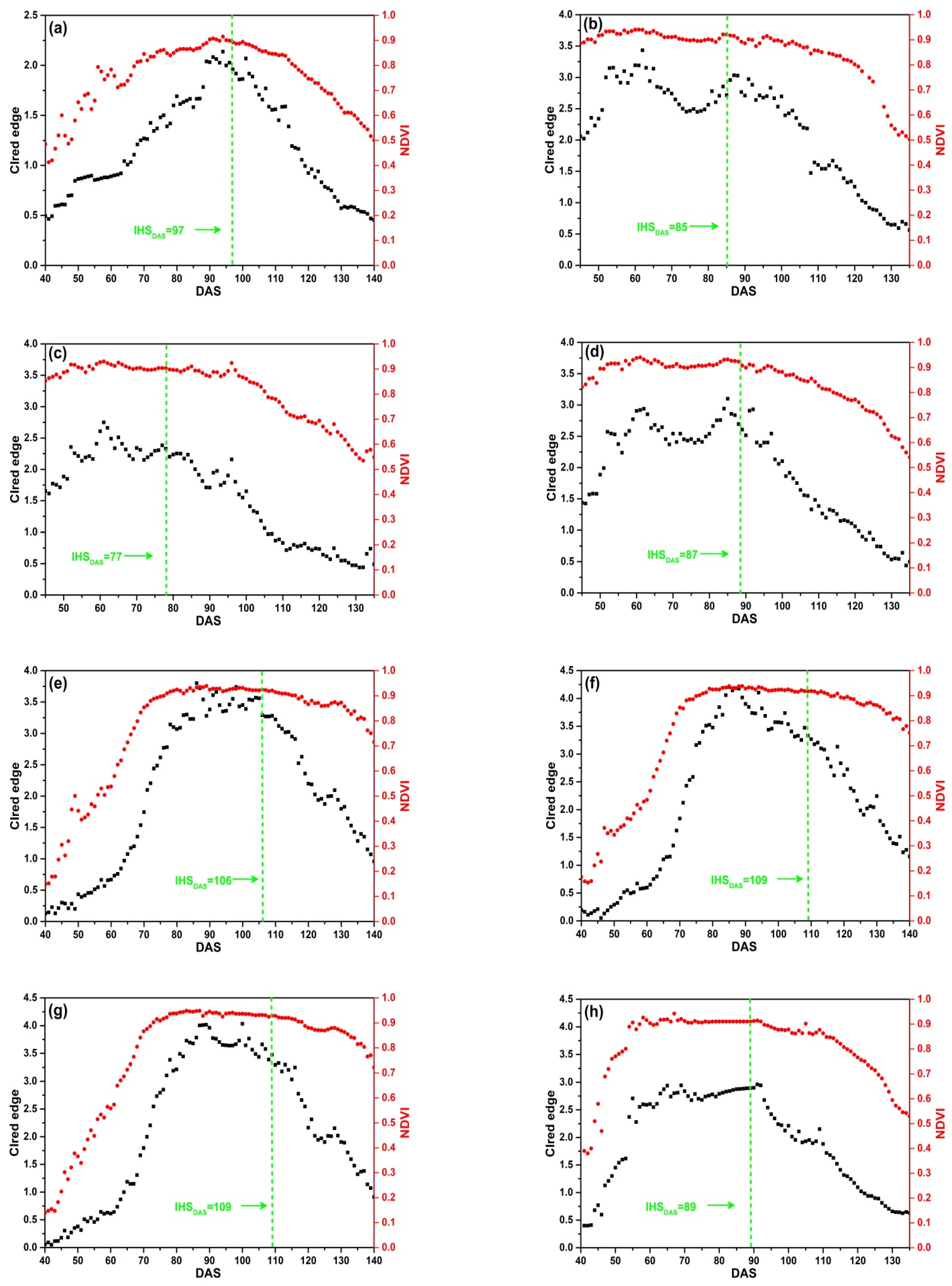
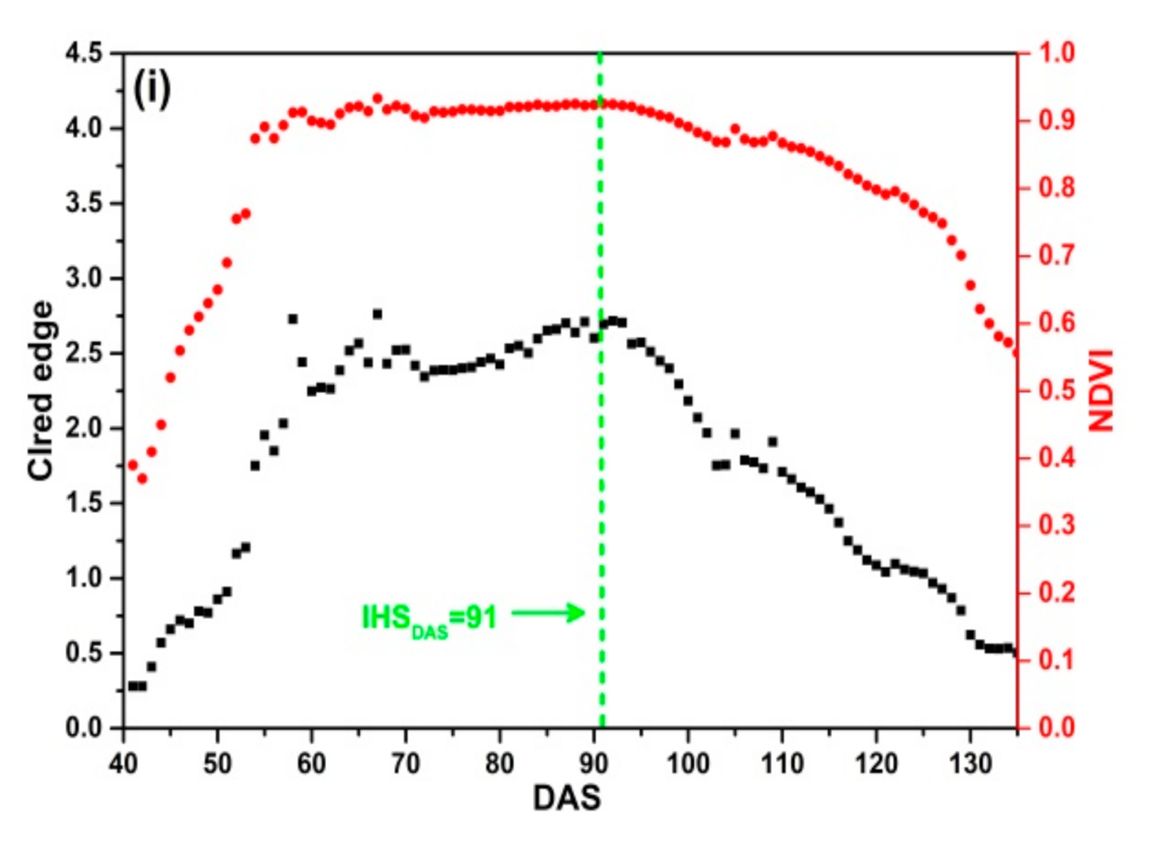
3.3. Comparative Analysis of Daily NDVI and CIred Edge

The SKYE radiometers were used to acquire daily reflectance data of 9 plots in four rice growing seasons. Figure 8 shows that the change regularity of NDVI is different from that of CIred edge. NDVI increases rapidly and achieves the maximum value quickly. Before DAS 70, NDVI increases rapidly; between DAS 80 to 100, NDVI remains stable and is close to 0.9. When rice is at maturity stage (after DAS 100), NDVI declines slowly with the senescence of leaves and stems, and it is close to 0.5 before harvesting. Especially, as Figure 8b–d present, NDVI achieves the maximum value before DAS 55 corresponding to the middle stage of tillering, which indicates that rice grows rapidly after transplanting in field. There is an obvious saturation problem occurring before IHS_DAS (the green lines in Figure 8). Thus, it is difficult to extract features from NDVI for monitoring IHS_DAS.

The curves of CIred edge are different in four rice growing seasons, but the change regularity of CIred edge is similar in the same growing season. CIred edge gradually increases with an exponential growth at tillering and jointing stage. CIred edge achieves the maximum value before IHS_DAS. The maximum value of CIred edge does not exceed 4 without saturation problem. CIred edge remains stable and is close to the maximum value before IHS_DAS. As shown in Figure 8, there are obvious inflection points of CIred edge appearing at IHS_DAS. It suggests that we can take advantage of the feature: the MC of time-series CIred edge for monitoring IHS_DAS. After IHS_DAS, CIred edge decreases linearly with the senescence of leaves and stems.

In addition, there is some noise in time-series CIred edge. For example, Figure 8b–d display abnormal fluctuations: two peaks and one trough appear between DAS 60 to 95. Thus, it is desirable to use some smoothing and fitting methods to eliminate noise of time-series CIred edge.

The comparative analysis indicates that CIred edge presents no saturation problem during the whole growth period of rice. CIred edge is better than NDVI for field-scale RP detection. Meanwhile, CIred edge has the obvious feature (MC) for monitoring IHS_DAS.

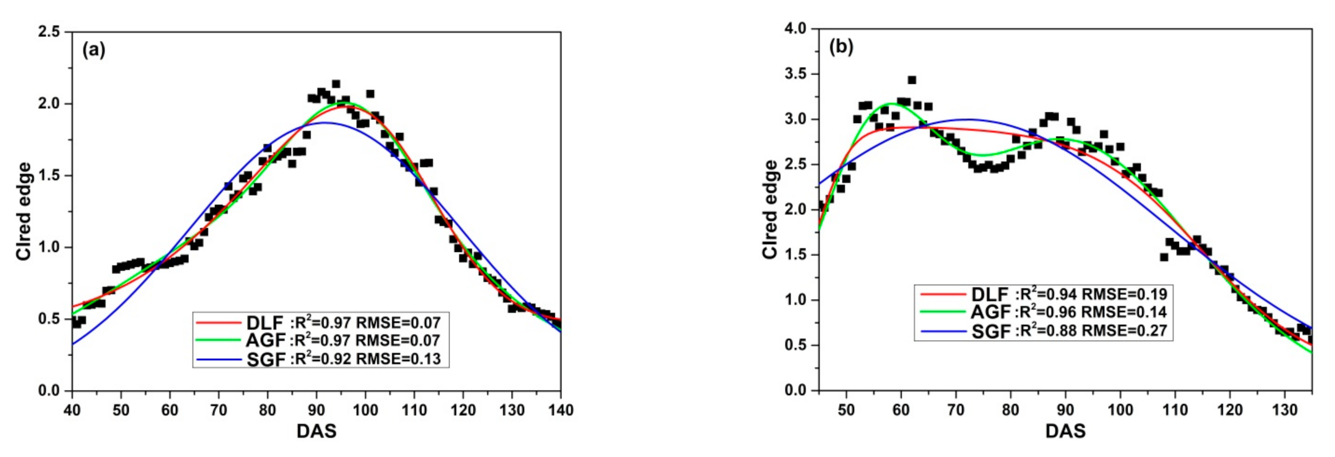
3.4. Fitting Several Source CIred Edge

3.4.1. Fitting CIred Edge of SKYE

Three fitting functions (DLF, AGF and SGF) are applied to fit CIred edge of SKYE in four growing seasons. Figure 9 illustrates the relationship between the original CIred edge and the fitted phenological curves. The results show that DLF, AGF and SGF can eliminate noise of the original CIred edge and help to present the change regularity of time-series CIred edge accurately. However, the performance of fitting models varies at different growth stages. DLF has good performance in fitting CIred edge at the early stages (before DAS 80). AGF is suitable to fit CIred edge between DAS 80 to 100, and SGF shows the highest accuracy after rice begins to grow into maturity (after DAS 100).

Table 8. The performance of the models in fitting CIred edge of SKYE.

Models	Fitting Function	R2	RMSE	Fitting Function	R2	RMSE	Fitting Function	R2	RMSE
a	DLF	0.97	0.07	AGF	0.97	0.07	SGF	0.92	0.13
b		0.94	0.19		0.96	0.14		0.88	0.27
c		0.96	0.13		0.96	0.14		0.94	0.16
d		0.94	0.17		0.95	0.16		0.91	0.22
e		0.98	0.13		0.98	0.14		0.95	0.23
f		0.98	0.14		0.98	0.13		0.92	0.36
g		0.98	0.14		0.98	0.15		0.95	0.28
h		0.97	0.14		0.96	0.15		0.89	0.26
i		0.96	0.15		0.97	0.14		0.89	0.25

summarizes the statistics (R² and RMSE) of three fitting models. For DLF models, R² varies between 0.94 and 0.98, RMSE ranges from 0.07 to 0.19. The model b shows the worst performance among DLF models, whereas the model e displays the best performance among DLF models. For AGF models, R² varies between 0.95 and 0.98, and RMSE ranges from 0.07 to 0.16. The model d shows the worst performance among AGF models, whereas the model f displays the best performance among AGF models. For SGF models, R² varies between 0.88 and 0.95, RMSE ranges from 0.13 to 0.36. The model b shows the worst performance among AGF models, whereas the model e displays the best performance among SGF models.

Overall, compared with AGF and SGF, DLF proves to have good performance in fitting CIred edge of SKYE during the whole growth period of rice.

3.4.2. Fitting CIred Edge of ASD

The performances of fitting models in four experiments are shown in

Table 9. The performance of the models in fitting CIred edge of ASD.

Experiment	Number of Plots	Fitting Functions	R2			RMSE
			Minimum	Mean	Maximum	Minimum	Mean	Maximum
1	n = 16	DLF	0.95	0.99	1	0	0.02	0.09
		AGF	1	1	1	0	0	0
		SGF	0.91	0.97	0.99	0.004	0.06	0.11
2	n = 52	DLF	0.84	0.98	1	0	0.05	0.18
		AGF	0.25	0.90	0.99	0.005	0.12	0.44
		SGF	0.62	0.89	0.98	0.08	0.16	0.29
3	n = 40	DLF	0.98	0.99	1	0	0.02	0.07
		AGF	0.92	0.98	0.99	0.01	0.08	0.19
		SGF	0.92	0.97	0.99	0.03	0.09	0.20
4	n = 24	DLF	0.97	0.99	1	0	0.03	0.12
		AGF	0.96	0.98	0.99	0.008	0.10	0.16
		SGF	0.95	0.97	0.99	0.07	0.12	0.17

. In experiment 1, R² and RMSE vary from 0.91–1 and 0–0.11. In experiment 2, R² and RMSE vary from 0.25–1 and 0–0.44. In experiment 3, R² and RMSE vary from 0.92–1 and 0–0.20. In experiment 4, R² and RMSE vary from 0.95–1 and 0–0.17.

We acquire 4, 6, 6, and 7 batches of CIred edge in experiments 1, 2, 3, and 4 (Table 4). There are six, six, and three parameters that need to be optimized in DLF, AGF, and SGF models. When the frequency of times for acquiring CIred edge is low, the over fitting problem of DLF and AGF models appears (R² = 1, RMSE = 0). Compared with DLF and AGF models, the accuracy of SGF models is lower in four experiments. However, there are no obvious over fitting problem appearing in SGF models. The results suggest that the fitting functions with fewer parameters, such as SGF, maybe suitable to avoid over fitting problem. SGF can reconstruct vegetation phenological curves using low-frequency CIred edge.

3.4.3. Fitting CIred Edge of MCA

Table 10. The performance of the models in fitting CIred edge of MCA.

Experiment	Number of Plots	Fitting Functions	R2			RMSE
			Minimum	Mean	Maximum	Minimum	Mean	Maximum
5	n = 1014	DLF	0.18	0.95	0.99	0.015	0.13	0.86
		AGF	0.32	0.92	0.99	0.02	0.19	0.90
		SGF	0.32	0.90	0.99	0.04	0.23	0.96
6	n = 289	DLF	0.69	0.96	0.99	0.05	0.16	0.34
		AGF	0.01	0.94	0.99	0.08	0.20	1.27
		SGF	0.24	0.91	0.98	0.15	0.27	0.47

summarizes the performance of DLF, AGF and SGF. For DLF models, R² varies between 0.18 and 0.99, RMSE ranges from 0.015 to 0.86. For AGF models, R² varies between 0.01 and 0.99, RMSE ranges from 0.02 to 1.27. For SGF models, R² varies between 0.24 and 0.99, RMSE ranges from 0.04 to 0.96. In addition, the performance evaluation implies that the fitting phenological curves (DLF_CIred edge, AGF_CIred edge and SGF_CIred edge) not only have a good correlation ship with the original CIred edge, but also can avoid over fitting problem (R² = 1, RMSE = 0).

In summary, compared with AGF and SGF, DLF is more suitable to fit time-series CIred edge of MCA, with higher R² and lower RMSE. This result is consistent with the result of SKYE data.

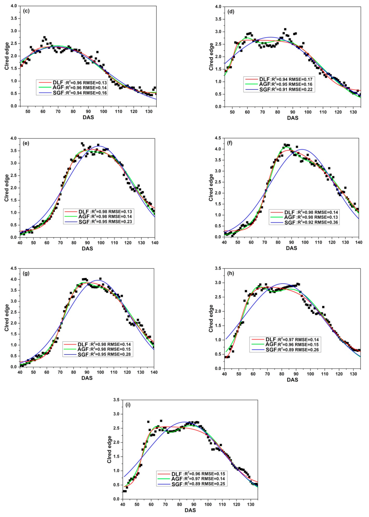
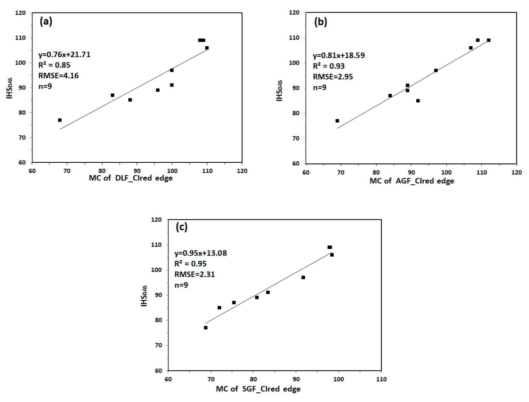
3.5. Monitoring IHS_DAS Based on Several Source CIred Edge

3.5.1. Monitoring IHS_DAS Based on CIred Edge of SKYE

We extracted the MC of DLF_CIred edge, AGF_CIred edge and SGF_CIred edge for monitoring IHS_DAS. Figure 10 shows the relationship between MC and IHS_DAS. MC of DLF_CIred edge has relatively lower correlation with IHS_DAS, with the values of R² and RMSE being 0.85 and 4.16. Compared with MC of DLF_CIred edge, MC of AGF_CIred edge and MC of SGF_CIred edge have good correlation with IHS_DAS, with R² values no less than 0.90, with RMSE values no more than 3.00. The results indicate that MC of CIred edge can be used to monitor IHS_DAS effectively.

3.5.2. Monitoring IHS_DAS Based on CIred Edge of ASD

Figure 11 shows the relationship between MC and IHS_DAS in experiment 1, 2, 3 and 4. MC of DLF_CIred edge and MC of AGF_CIred edge have the lowest correlation with IHS_DAS, with R² values of 0.46 and 0.46, RMSE values of 9.18 and 9.23. MC of SGF_CIred edge proves to have good fitting characteristics for monitoring IHS_DAS, with the values of R² and RMSE being 0.95 and 2.86.

3.5.3. Monitoring IHS_DAS Based on CIred Edge of MCA

Figure 12 shows the relationship between MC and IHS_DAS in experiment 5 and 6. MC of DLF_CIred edge and MC of AGF_CIred edge have the lowest correlation with IHS_DAS, with R² values of 0.43 and 0.45, RMSE values of 6.90 and 6.76. MC of SGF_CIred edge has good correlation with IHS_DAS, with the values of R² and RMSE being 0.82 and 3.81. The results are consistent with the results based on CIred edge of ASD.

3.6. Effects of Rice Cultivars and N Rates on IHS_DAS

In order to understand the influence of rice cultivars and N rates on IHS_DAS, experiment 4 was conducted in a randomized complete block designed with three replications for each treatment, involving two rice cultivars (FLY4 and LY9348) and four N rates (N0, N1, N2 and N3). The analysis of variance (ANOVA) indicates that rice cultivars and N rates have obvious effects on IHS_DAS (

Table 11. Analysis of variance (ANOVA) of IHS_DAS.

Experiment	Variable	Factor	Degree of Freedom	Sum of Squares	Mean Square	F Value
4	IHSDAS	Rice Cultivars	1	1.50	1.50	5.14 *
	IHSDAS	N rates	3	95.17	31.72	108.76 **
	IHSDAS	Rice Cultivars × N rates	3	4.50	1.50	5.14 *

Note: * denotes the significant level of α = 0.05, ** denotes the extremely significant level of α = 0.01.

). There is a significant difference between LY9348 and FLY4. The difference of IHS_DAS reaches an extremely significant level under different N rates. The interaction of different rice cultivars and N rates on IHS_DAS reaches a significant level. The ANOVA suggests that we would better take into account rice cultivars and N rates when monitoring IHS_DAS.

Figure 13 shows that IHS_DAS of FLY4 are larger than that of LY9348 under same N rates. Under N1, the average IHS_DAS of FLY4 and LY9348 are 104.66 and 103.66. While under N3, IHS_DAS of FLY 4 and LY 9348 are 110 and 109. With the increase of nitrogen fertilizer application, IHS_DAS of LY9348 and FLY4 increase correspondingly, the results are consistent with previous study [70]. In general, when using more nitrogen fertilizer before heading and flowering stage, the rice growth process might be delayed, leaves would remain green, and spikes appeared later, resulting in a longer life cycle of rice.

4. Discussion

4.1. Daily CIred Edge for Monitoring RP

Previous studies showed that time-series NDVI was suitable for monitoring vegetation phenology [71,72]. However, the major problem of NDVI was that it became saturated for vegetation with moderate to high density [73]. Our study confirmed this fact: daily NDVI of SKYE became significantly saturated before flowers and spikes appeared in rice. Thus, it was difficult to extract features from NDVI for monitoring IHS_DAS. In comparison with NDVI, daily CIred edge of SKYE had no saturation problem during the whole rice growth stage, and was more suitable for monitoring IHS_DAS.

Figure 8 showed that the change regularity of daily CIred edge was closely related to the actual growth process of rice. To our knowledge, CIred edge was originally proposed for high accuracy chlorophyll estimation [74], some studies have demonstrated that the canopy chlorophyll content was closely related to vegetation growth period [75,76]. Therefore CIred edge was better than NDVI for monitoring RP, and the result was consistent with the previous study [9].

In addition, the maximum air temperature (Tmax) has a significant effect on daily CIred edge. Figure 14 displays daily ${\rho }_{NIR}$ and ${\rho }_{Red edge}$ of C_SKYE and Tmax in Ezhou city and Lingshui city. In Lingshui city, Tmax is stable and always below 35 °C. However, the continuous high air temperature (Tmax ≥ 35 °C) often appears with drastic change in Ezhou city. The abnormal change of ${\rho }_{NIR}$ often occurs between DAS 60 to 95 when Tmax has drastic change (Figure 14a). Meanwhile, the abnormal CIred edge also appeared between DAS 60 to 95 (Figure 8d). In general, rice canopy reflectance presents a spectral curve of typical green vegetation before IHS_DAS, ${\rho }_{Red edge}$ is much lower than ${\rho }_{NIR}$ during different growth stage [77,78]. In our study, compared with ${\rho }_{NIR}$, ${\rho }_{Red edge}$ slowly increases with the progress of rice growth and is not sensitive to high air temperature. However, the drastic change of Tmax could cause the sudden change of ${\rho }_{NIR}$, resulting in the abnormal fluctuation of CIred edge appearing.

Rice is a crop that is sensitive to high temperature [79] and water [80]. The continuous high air temperature or additional rain had great influence on the growth process of rice, IHS_DAS of rice may be advanced or postponed [81]. Moreover, strong sunlight can burn rice leaves and change the rice canopy structure. Thus, it is better to take measures (smooth and fitting methods) to eliminate noise before time-series CIred edge was applied to monitor RP. VIs were indeed an effective tool for monitoring vegetation phenology [82,83]. However, if we can make better use of other information, for example, texture, three-dimensional information and coverage, the accuracy of monitoring RP will be improved in the future [84].

4.2. Comparative Analysis of DLF, AGF and SGF for Fitting Several Source CIred Edge

In order to obtain high quality time-series CIred edge, we used DLF, AGF, and SGF to fit CIred edge. The results indicated that DLF and AGF proved to have good performance in fitting CIred edge of SKYE and MCA with higher R² and lower RMSE. However, when the frequency of times for acquiring CIred edge is low, Table 9 shows that the over fitting problem (R² = 1, RMSE = 0) of DLF and AGF models appears. Compared with DLF and AGF models, SGF models have a lower correlation ship with the original CIred edge of ASD, but without obvious over fitting problem.

There are six, six, and three parameters that need to be optimized in DLF, AGF, and SGF models. DLF and AGF are relatively complex, more parameters mean that more CIred edge data should be put into DLF and AGF models. Low-frequency measured data was more likely to cause over fitting problem when more parameters need to be optimized in fitting functions. As we know, the over fitting problem may misinterpret important phenological features and directly affect the accuracy of monitoring vegetation phenology [52]. Thus, DLF and AGF are not suitable to fit low-frequency CIred edge. Acquiring high-frequency CIred edge will help to highlight the phenological features for monitoring RP.

Overall, DLF and AGF could be effectively applied to fit dense CIred edge with higher R² and lower RMSE, and to describe more detailed changes of rice canopy at different growth stages. SGF had good performance in fitting low-frequency CIred edge.

4.3. Monitoring IHS_DAS Based on Several Source CIred Edge

Time-series CIred edge from SKYE, ASD and MCA were reconstructed by DLF, AGF and SGF. We extracted the features: MC of DLF_CIred edge, AGF_CIred edge and SGF_CIred edge for monitoring IHS_DAS.

MC of DLF_CIred edge and AGF_CIred edge from SKYE had good correlation with IHS_DAS. However, MC of DLF_CIred edge and AGF_CIred edge from ASD and MCA did not perform well for monitoring IHS_DAS. MC of SGF_CIred edge from three platforms all have good performance in monitoring IHS_DAS, R² varies between 0.82 and 0.95, RMSE ranges from 2.31 to 3.81, which means that MC of SGF_CIred edge could be applied to monitor IHS_DAS with good robustness. The rice flowers and spikes were usually bright yellow with contrasting colour to the rice leaves [49]. The chlorophyll content of flowers and spikes were also lower than that of green leaves. After flowers and spikes came out, the canopy chlorophyll of rice would decrease dramatically, resulting in the obvious inflection points of CIred edge appearing at IHS_DAS. Thereby, the MC of time-series CIred edge was an essential feature for monitoring field-scale IHS_DAS.

In this study, the accuracy of monitoring IHS_DAS was different using MC extracted from three low-altitude remote sensing data. Three different platforms have the advantages and disadvantages. SKYE radiometers could continuously collect in situ field-scale rice canopy reflectance at very high temporal resolution, which helped analyze the change regularity of phenological curves and extract features for monitoring RP. However, they were mounted in the fixed positions for monitoring several fields, lacking mobility and flexibility [85]. ASD had wider spectrum range and high radiation resolution for extracting accurate VIs, but it was time-consuming to acquire the hyperspectral reflectance of different rice cultivars. The multispectral UAV system had the advantages of mobility, it could collect multispectral images for monitoring real-time large-scale vegetation growth [56,86,87,88]. However, the processing flow of multispectral image was relatively complicated, including radiometric calibration, geometric correction, and image mosaic. It is necessary to acquire the high spatiotemporal and hyperspectral data for improving the accuracy of monitoring field-scale IHS_DAS.

4.4. The Influence Factors on IHS_DAS

There were many factors influencing vegetation phenology, such as illumination, air temperature, vegetation varieties and fertilizer application [89,90]. In our study, we mainly took into account rice cultivars, N rates and air temperature for monitoring IHS_DAS. Table 11 indicates that rice cultivars and N rates have obvious effects on IHS_DAS. The interaction of different rice cultivars and N rates on the IHS_DAS reaches significant level. With the increase of N rates, IHS_DAS of LY 9348 and FLY 4 both increase, which indicates that the growth process of rice is delayed when more nitrogen fertilizer is applied before heading stage, and leaves would remain green, flowers and spikes appear later [70]. In a word, rice cultivars and nitrogen fertilizer application have great influence on RP [91,92].

Air temperature could not only affect the near infrared reflectance, but also disturb RP. Compared with Lingshui city, the weather of Ezhou city fluctuates greatly, it often remains continuous high temperature (T_max ≥ 35 °C). Table 3 shows that IHS_DAS of LY 9348 and FLY 4 planted in Ezhou city are lower than that in Lingshui city. The results confirm that high air temperature might accelerate the whole growth process of rice and shorten growth duration [93,94,95]. The IHS_DAS of hybrid rice might decrease when the same rice cultivars are planted in high temperature area.

5. Conclusions

In this study, we presented the processing steps for monitoring hybrid rice IHS_DAS based on three low-altitude remote sensing data and analyzed the influential factors (rice cultivars, N rates, and air temperature) of RP.

The results indicated that CIred edge could show hybrid rice phenological change accurately without saturation problem, and was more appropriate than NDVI for monitoring IHS_DAS. SGF could eliminate the noise of time series CIred edge without over fitting problem. MC of SGF_CIred edge from three low-altitude remote sensing platforms had good performance in monitoring IHS_DAS with good robustness, as R² varied between 0.82 and 0.95 and RMSE ranged from 2.31 to 3.81.

This study demonstrated that high air temperature might cause a decrease of IHS_DAS when the same rice cultivars were planted in high temperature area. In addition, the interaction of different rice cultivars and N rates on IHS_DAS reached a significant level. The growth process of rice was delayed when more nitrogen fertilizer was applied before IHS_DAS.

Future work should evaluate these results for diverse rice cultivars under different environmental conditions, by combing low-altitude remote sensing data and satellite data. In addition, new methods for reconstructing rice phenological curves will be explored for monitoring RP in the future. We expect that our study will provide useful guidance for breeding rice and fertilizer management with remote sensing technology.

References

1. Kuenzer, C.; Knauer, K. Remote sensing of rice crop areas. Int. J. Remote Sens. 2013, 34, 2101–2139. [Google Scholar] [CrossRef]
2. Wang, H.; Deng, X.W. Development of the “Third-Generation” Hybrid Rice in China. Genom. Proteom. Bioinform. 2018, 16, 393–396. [Google Scholar] [CrossRef]
3. Kempe, K.; Gils, M. Pollination control technologies for hybrid breeding. Mol. Breed. 2011, 27, 417–437. [Google Scholar] [CrossRef]
4. Cheng, S.H.; Zhuang, J.Y.; Fan, Y.Y.; Du, J.H.; Cao, L.Y. Progress in research and development on hybrid rice: A super-domesticate in china. Ann. Bot. 2007, 100, 959–966. [Google Scholar] [CrossRef] [PubMed]
5. Huang, X.; Yang, S.; Gong, J.; Zhao, Y.; Feng, Q.; Gong, H.; Li, W.; Zhan, Q.; Cheng, B.; Xia, J.; et al. Genomic analysis of hybrid rice varieties reveals numerous superior alleles that contribute to heterosis. Nat. Commun. 2015, 6, 7258. [Google Scholar] [CrossRef] [PubMed] [Green Version]
6. Peng, S. Dilemma and Way-out of Hybrid Rice during the Transition Period in China. Acta Agron. Sin. 2016, 42, 313–319. [Google Scholar] [CrossRef]
7. Zhou, X.; Zheng, H.B.; Xu, X.Q.; He, J.Y.; Ge, X.K.; Yao, X.; Cheng, T.; Zhu, Y.; Cao, W.X.; Tian, Y.C. Predicting grain yield in rice using multi-temporal vegetation indices from UAV-based multispectral and digital imagery. ISPRS J. Photogramm. Remote Sens. 2017, 130, 246–255. [Google Scholar] [CrossRef]
8. Yang, Z.; Shao, Y.; Li, K.; Liu, Q.; Liu, L.; Brisco, B. An improved scheme for rice phenology estimation based on time-series multispectral HJ-1A/B and polarimetric RADARSAT-2 data. Remote Sens. Environ. 2017, 195, 184–201. [Google Scholar] [CrossRef]
9. Zheng, H.; Cheng, T.; Yao, X.; Deng, X.; Tian, Y.; Cao, W.; Zhu, Y. Detection of rice phenology through time series analysis of ground-based spectral index data. Field Crops Res. 2016, 198, 131–139. [Google Scholar] [CrossRef]
10. Li, J.; Zhou, J.W.; Xu, P.; Deng, X.N.; Deng, W.; Zhang, Y.; Yang, Y.; Tao, D.Y. Mapping five novel interspecific hybrid sterility loci between Oryza sativa and Oryza meridionalis. Breed. Sci. 2018, 68, 516–523. [Google Scholar] [CrossRef] [Green Version]
11. Guo, T.; Yu, X.; Li, X.; Zhang, H.; Zhu, C.; Flint-Garcia, S.; McMullen, M.D.; Holland, J.B.; Szalma, S.J.; Wisser, R.J.; et al. Optimal Designs for Genomic Selection in Hybrid Crops. Mol. Plant 2019, 12, 390–401. [Google Scholar] [CrossRef] [PubMed] [Green Version]
12. Guo, W.; Fukatsu, T.; Ninomiya, S. Automated characterization of flowering dynamics in rice using field-acquired time-series RGB images. Plant Methods 2015, 11, 7. [Google Scholar] [CrossRef] [PubMed] [Green Version]
13. Li, J.; Lan, Y.; Wang, J.; Chen, S.; Huang, C.; Liu, Q.; Liang, Q. Distribution law of rice pollen in the wind field of small UAV. Int. J. Agric. Biol. Eng. 2017, 10, 32–40. [Google Scholar] [CrossRef]
14. Yabe, S.; Nakagawa, H.; Adachi, S.; Mukouyama, T.; Arai-Sanoh, Y.; Okamura, M.; Kondo, M.; Yoshida, H. Model analysis of genotypic difference in the variation of the duration from heading to flower opening based on the flower position on a panicle in high-yielding rice cultivars. Field Crops Res. 2018, 223, 155–163. [Google Scholar] [CrossRef]
15. Wan, L.; Cen, H.; Zhu, J.; Zhang, J.; Zhu, Y.; Sun, D.; Du, X.; Zhai, L.; Weng, H.; Li, Y.; et al. Grain yield prediction of rice using multi-temporal UAV-based RGB and multispectral images and model transfer—A case study of small farmlands in the South of China. Agric. For. Meteorol. 2020, 291, 108096. [Google Scholar] [CrossRef]
16. Piao, S.; Liu, Q.; Chen, A.; Janssens, I.A.; Fu, Y.; Dai, J.; Liu, L.; Lian, X.; Shen, M.; Zhu, X. Plant phenology and global climate change: Current progresses and challenges. Glob. Chang. Biol. 2019. [Google Scholar] [CrossRef] [PubMed]
17. Gao, Y.; Wallach, D.; Liu, B.; Dingkuhn, M.; Boote, K.J.; Singh, U.; Asseng, S.; Kahveci, T.; He, J.; Zhang, R.; et al. Comparison of three calibration methods for modeling rice phenology. Agric. For. Meteorol. 2020, 280, 107785. [Google Scholar] [CrossRef]
18. Weil, G.; Lensky, I.M.; Levin, N. Using ground observations of a digital camera in the VIS-NIR range for quantifying the phenology of Mediterranean woody species. Int. J. Appl. Earth Obs. Geoinf. 2017, 62, 88–101. [Google Scholar] [CrossRef]
19. Gnyp, M.L.; Miao, Y.; Yuan, F.; Ustin, S.L.; Yu, K.; Yao, Y.; Huang, S.; Bareth, G. Hyperspectral canopy sensing of paddy rice aboveground biomass at different growth stages. Field Crops Res. 2014, 155, 42–55. [Google Scholar] [CrossRef]
20. Zhang, S.; Tao, F. Modeling the response of rice phenology to climate change and variability in different climatic zones: Comparisons of five models. Eur. J. Agron. 2013, 45, 165–176. [Google Scholar] [CrossRef]
21. Kim, M.; Ko, J.; Jeong, S.; Yeom, J.-m.; Kim, H.-o. Monitoring canopy growth and grain yield of paddy rice in South Korea by using the GRAMI model and high spatial resolution imagery. Gisci. Remote Sens. 2017, 54, 534–551. [Google Scholar] [CrossRef]
22. Weir, A.H.; Bragg, P.L.; Porter, J.R.; Rayner, J.H. A winter-wheat crop simulation-model without water or nutrient limitations. J. Agric. Sci. 1984, 102, 371–382. [Google Scholar] [CrossRef]
23. Wu, L.; Liu, X.; Zhou, B.; Li, L.; Tan, Z. Spatial-time continuous changes simulation of crop growth parameters with multi-source remote sensing data and crop growth model. J. Remote Sens. 2012, 16, 1173–1191. [Google Scholar]
24. Villa, P.; Pinardi, M.; Bolpagni, R.; Gillier, J.-M.; Zinke, P.; Nedelcuţ, F.; Bresciani, M. Assessing macrophyte seasonal dynamics using dense time series of medium resolution satellite data. Remote Sens. Environ. 2018, 216, 230–244. [Google Scholar] [CrossRef]
25. Zhang, X.; Friedl, M.A.; Schaaf, C.B.; Strahler, A.H.; Hodges, J.C.F.; Gao, F.; Reed, B.C.; Huete, A. Monitoring vegetation phenology using MODIS. Remote Sens. Environ. 2003, 84, 471–475. [Google Scholar] [CrossRef]
26. Zhang, S.; Tao, F. Improving rice development and phenology prediction across contrasting climate zones of China. Agric. For. Meteorol. 2019, 268, 224–233. [Google Scholar] [CrossRef]
27. Xie, Y.Y.; Civco, D.L.; Silander, J.A. Species-specific spring and autumn leaf phenology captured by time-lapse digital cameras. Ecosphere 2018, 9. [Google Scholar] [CrossRef] [Green Version]
28. Xu, J.; Meng, J.; Quackenbush, L.J. Use of remote sensing to predict the optimal harvest date of corn. Field Crops Res. 2019, 236, 1–13. [Google Scholar] [CrossRef]
29. Ma, Y.; Fang, S.; Peng, Y.; Gong, Y.; Wang, D. Remote Estimation of Biomass in Winter Oilseed Rape (Brassica napus L.) Using Canopy Hyperspectral Data at Different Growth Stages. Appl. Sci. 2019, 9, 545. [Google Scholar] [CrossRef] [Green Version]
30. Quan, X.; He, B.; Yebra, M.; Yin, C.; Liao, Z.; Zhang, X.; Li, X. A radiative transfer model-based method for the estimation of grassland aboveground biomass. Int. J. Appl. Earth Obs. Geoinf. 2017, 54, 159–168. [Google Scholar] [CrossRef]
31. Vrieling, A.; Meroni, M.; Darvishzadeh, R.; Skidmore, A.K.; Wang, T.; Zurita-Milla, R.; Oosterbeek, K.; O’Connor, B.; Paganini, M. Vegetation phenology from Sentinel-2 and field cameras for a Dutch barrier island. Remote Sens. Environ. 2018, 215, 517–529. [Google Scholar] [CrossRef]
32. Wang, Y.F.; Xue, Z.H.; Chen, J.; Chen, G.Z. Spatio-temporal analysis of phenology in Yangtze River Delta based on MODIS NDVI time series from 2001 to 2015. Front. Earth Sci. 2019, 13, 92–110. [Google Scholar] [CrossRef]
33. Sakamoto, T.; Yokozawa, M.; Toritani, H.; Shibayama, M.; Ishitsuka, N.; Ohno, H. A crop phenology detection method using time-series MODIS data. Remote Sens. Environ. 2005, 96, 366–374. [Google Scholar] [CrossRef]
34. Onojeghuo, A.O.; Blackburn, G.A.; Wang, Q.; Atkinson, P.M.; Kindred, D.; Miao, Y. Rice crop phenology mapping at high spatial and temporal resolution using downscaled MODIS time-series. GIScience Remote Sens. 2018, 55, 659–677. [Google Scholar] [CrossRef] [Green Version]
35. Sun, N.; Wang, P.; Huang, F.; Li, B. Developing an integrated index based on phenological metrics for evaluating cadmium stress in rice using Sentinel-2 data. J. Appl. Remote Sens. 2018, 12, 036018. [Google Scholar] [CrossRef]
36. Ricotta, C.; Avena, G.C. The remote sensing approach in broad-scale phenological studies. Appl. Veg. Sci. 2000, 3, 117–122. [Google Scholar] [CrossRef]
37. White, M.A.; Hoffman, F.; Hargrove, W.W.; Nemani, R.R. A global framework for monitoring phenological responses to climate change. Geophys. Res. Lett. 2005, 32. [Google Scholar] [CrossRef] [Green Version]
38. Wang, H.; Magagi, R.; Goïta, K.; Trudel, M.; McNairn, H.; Powers, J. Crop phenology retrieval via polarimetric SAR decomposition and Random Forest algorithm. Remote Sens. Environ. 2019, 231, 111234. [Google Scholar] [CrossRef]
39. Hirooka, Y.; Homma, K.; Maki, M.; Sekiguchi, K. Applicability of synthetic aperture radar (SAR) to evaluate leaf area index (LAI) and its growth rate of rice in farmers’ fields in Lao PDR. Field Crops Res. 2015, 176, 119–122. [Google Scholar] [CrossRef] [Green Version]
40. Fikriyah, V.N.; Darvishzadeh, R.; Laborte, A.; Khan, N.I.; Nelson, A. Discriminating transplanted and direct seeded rice using Sentinel-1 intensity data. Int. J. Appl. Earth Obs. Geoinf. 2019, 76, 143–153. [Google Scholar] [CrossRef] [Green Version]
41. Lopez-Sanchez, J.M.; Cloude, S.R.; Ballester-Berman, J.D. Rice Phenology Monitoring by Means of SAR Polarimetry at X-Band. IEEE Trans. Geosci. Remote Sens. 2012, 50, 2695–2709. [Google Scholar] [CrossRef]
42. Yuzugullu, O.; Erten, E.; Hajnsek, I. Rice Growth Monitoring by Means of X-Band Co-polar SAR: Feature Clustering and BBCH Scale. IEEE Geosci. Remote Sens. Lett. 2015, 12, 1218–1222. [Google Scholar] [CrossRef]
43. He, Z.; Li, S.H.; Wang, Y.; Dai, L.Y.; Lin, S. Monitoring Rice Phenology Based on Backscattering Characteristics of Multi-Temporal RADARSAT-2 Datasets. Remote Sens. 2018, 10, 340. [Google Scholar] [CrossRef] [Green Version]
44. Bendig, J.; Yu, K.; Aasen, H.; Bolten, A.; Bennertz, S.; Broscheit, J.; Gnyp, M.L.; Bareth, G. Combining UAV-based plant height from crop surface models, visible, and near infrared vegetation indices for biomass monitoring in barley. Int. J. Appl. Earth Obs. Geoinf. 2015, 39, 79–87. [Google Scholar] [CrossRef]
45. Graham, E.A.; Riordan, E.C.; Yuen, E.M.; Estrin, D.; Rundel, P.W. Public Internet-connected cameras used as a cross-continental ground-based plant phenology monitoring system. Glob. Chang. Biol. 2010, 16, 3014–3023. [Google Scholar] [CrossRef]
46. Li, L.; Ren, T.; Ma, Y.; Wei, Q.; Wang, S.; Li, X.; Cong, R.; Liu, S.; Lu, J. Evaluating chlorophyll density in winter oilseed rape (Brassica napus L.) using canopy hyperspectral red-edge parameters. Comput. Electron. Agric. 2016, 126, 21–31. [Google Scholar] [CrossRef]
47. Zhou, M.; Ma, X.; Wang, K.; Cheng, T.; Tian, Y.; Wang, J.; Zhu, Y.; Hu, Y.; Niu, Q.; Gui, L.; et al. Detection of phenology using an improved shape model on time-series vegetation index in wheat. Comput. Electron. Agric. 2020, 173, 105398. [Google Scholar] [CrossRef]
48. Yang, Q.; Shi, L.; Han, J.; Yu, J.; Huang, K. A near real-time deep learning approach for detecting rice phenology based on UAV images. Agric. For. Meteorol. 2020, 287, 107938. [Google Scholar] [CrossRef]
49. Bai, X.; Cao, Z.; Zhao, L.; Zhang, J.; Lv, C.; Li, C.; Xie, J. Rice heading stage automatic observation by multi-classifier cascade based rice spike detection method. Agric. For. Meteorol. 2018, 259, 260–270. [Google Scholar] [CrossRef]
50. Wang, L.; Zhang, F.-C.; Jing, Y.-S.; Jiang, X.-D.; Yang, S.-B.; Han, X.-M. Multi-Temporal Detection of Rice Phenological Stages Using Canopy Spectrum. Rice Sci. 2014, 21, 108–115. [Google Scholar] [CrossRef]
51. Han, J.; Shi, L.; Yang, Q.; Huang, K.; Zha, Y.; Yu, J. Real-time detection of rice phenology through convolutional neural network using handheld camera images. Precis. Agric. 2020. [Google Scholar] [CrossRef]
52. Zeng, L.; Wardlow, B.D.; Xiang, D.; Hu, S.; Li, D. A review of vegetation phenological metrics extraction using time-series, multispectral satellite data. Remote Sens. Environ. 2020, 237, 111511. [Google Scholar] [CrossRef]
53. Baugh, W.M.; Groeneveld, D.P. Empirical proof of the empirical line. Int. J. Remote Sens. 2008, 29, 665–672. [Google Scholar] [CrossRef]
54. Duan, B.; Liu, Y.; Gong, Y.; Peng, Y.; Wu, X.; Zhu, R.; Fang, S. Remote estimation of rice LAI based on Fourier spectrum texture from UAV image. Plant Methods 2019, 15. [Google Scholar] [CrossRef] [Green Version]
55. Laliberte, A.S.; Goforth, M.A.; Steele, C.M.; Rango, A. Multispectral Remote Sensing from Unmanned Aircraft: Image Processing Workflows and Applications for Rangeland Environments. Remote Sens. 2011, 3, 2529–2551. [Google Scholar] [CrossRef] [Green Version]
56. Deng, L.; Mao, Z.; Li, X.; Hu, Z.; Duan, F.; Yan, Y. UAV-based multispectral remote sensing for precision agriculture: A comparison between different cameras. ISPRS J. Photogramm. Remote Sens. 2018, 146, 124–136. [Google Scholar] [CrossRef]
57. Haiying, L.; Hongchun, Z. Hyperspectral characteristic analysis for leaf nitrogen content in different growth stages of winter wheat. Appl. Opt. 2016, 55, D151–D161. [Google Scholar] [CrossRef]
58. Rouse, J.W., Jr.; Haas, R.; Schell, J.; Deering, D. Monitoring Vegetation Systems in the Great Plains with ERTS; NASA/GSFCT Type III Final Report; National Aeronautics and Space Administration (NASA): Washington, DC, USA, 1974; pp. 309–317.
59. Gitelson, A.A.; Gritz, Y.; Merzlyak, M.N. Relationships between leaf chlorophyll content and spectral reflectance and algorithms for non-destructive chlorophyll assessment in higher plant leaves. J. Plant Physiol. 2003, 160, 271–282. [Google Scholar] [CrossRef]
60. Minoli, S.; Egli, D.B.; Rolinski, S.; Müller, C. Modelling cropping periods of grain crops at the global scale. Glob. Planet. Chang. 2019, 174, 35–46. [Google Scholar] [CrossRef]
61. Ishikawa, D.; Hoogenboom, G.; Hakoyama, S.; Ishiguro, E. A potential of the growth stage estimation for paddy rice by using chlorophyll absorption bands in the 400–1100 nm region. J. Agric. Meteorol. 2015, 71, 24–31. [Google Scholar] [CrossRef] [Green Version]
62. De Castro, I.A.; Six, J.; Plant, E.R.; Peña, M.J. Mapping Crop Calendar Events and Phenology-Related Metrics at the Parcel Level by Object-Based Image Analysis (OBIA) of MODIS-NDVI Time-Series: A Case Study in Central California. Remote Sens. 2018, 10, 1745. [Google Scholar] [CrossRef] [Green Version]
63. Kandasamy, S.; Baret, F.; Verger, A.; Neveux, P.; Weiss, M. A comparison of methods for smoothing and gap filling time series of remote sensing observations-application to MODIS LAI products. Biogeosciences 2013, 10, 4055–4071. [Google Scholar] [CrossRef] [Green Version]
64. Jonsson, P.; Eklundh, L. Seasonality extraction by function fitting to time-series of satellite sensor data. IEEE Trans. Geosci. Remote Sens. 2002, 40, 1824–1832. [Google Scholar] [CrossRef]
65. Atkinson, P.M.; Jeganathan, C.; Dash, J.; Atzberger, C. Inter-comparison of four models for smoothing satellite sensor time-series data to estimate vegetation phenology. Remote Sens. Environ. 2012, 123, 400–417. [Google Scholar] [CrossRef]
66. Beck, P.S.A.; Atzberger, C.; Hogda, K.A.; Johansen, B.; Skidmore, A.K. Improved monitoring of vegetation dynamics at very high latitudes: A new method using MODIS NDVI. Remote Sens. Environ. 2006, 100, 321–334. [Google Scholar] [CrossRef]
67. Hird, J.N.; McDermid, G.J. Noise reduction of NDVI time series: An empirical comparison of selected techniques. Remote Sens. Environ. 2009, 113, 248–258. [Google Scholar] [CrossRef]
68. Zhang, X.; Liu, L.; Henebry, G.M. Impacts of land cover and land use change on long-term trend of land surface phenology: A case study in agricultural ecosystems. Environ. Res. Lett. 2019, 14, 044020. [Google Scholar] [CrossRef] [Green Version]
69. Jonsson, P.; Eklundh, L. TIMESAT—A program for analyzing time-series of satellite sensor data. Comput. Geosci. 2004, 30, 833–845. [Google Scholar] [CrossRef] [Green Version]
70. Liu, H.; Won, P.L.P.; Banayo, N.P.M.; Nie, L.; Peng, S.; Kato, Y. Late-season nitrogen applications improve grain yield and fertilizer-use efficiency of dry direct-seeded rice in the tropics. Field Crops Res. 2019, 233, 114–120. [Google Scholar] [CrossRef]
71. Li, X.; Zhou, Y.; Meng, L.; Asrar, G.; Sapkota, A.; Coates, F. Characterizing the relationship between satellite phenology and pollen season: A case study of birch. Remote Sens. Environ. 2019, 222, 267–274. [Google Scholar] [CrossRef]
72. Haerani, H.; Apan, A.; Basnet, B. Mapping of peanut crops in Queensland, Australia, using time-series PROBA-V 100-m normalized difference vegetation index imagery. J. Appl. Remote Sens. 2018, 12, 036005. [Google Scholar] [CrossRef]
73. Wang, C.; Feng, M.-C.; Yang, W.-D.; Ding, G.-W.; Sun, H.; Liang, Z.-Y.; Xie, Y.-K.; Qiao, X.-X. Impact of spectral saturation on leaf area index and aboveground biomass estimation of winter wheat. Spectrosc. Lett. 2016, 49, 241–248. [Google Scholar] [CrossRef]
74. Gitelson, A.A.; Peng, Y.; Vina, A.; Arkebauer, T.; Schepers, J.S. Efficiency of chlorophyll in gross primary productivity: A proof of concept and application in crops. J. Plant Physiol. 2016, 201, 101–110. [Google Scholar] [CrossRef] [PubMed] [Green Version]
75. Kanning, M.; Kühling, I.; Trautz, D.; Jarmer, T. High-Resolution UAV-Based Hyperspectral Imagery for LAI and Chlorophyll Estimations from Wheat for Yield Prediction. Remote Sens. 2018, 10, 2000. [Google Scholar] [CrossRef] [Green Version]
76. Yu, K.; Lenz-Wiedemann, V.; Chen, X.; Bareth, G. Estimating leaf chlorophyll of barley at different growth stages using spectral indices to reduce soil background and canopy structure effects. ISPRS J. Photogramm. Remote Sens. 2014, 97, 58–77. [Google Scholar] [CrossRef]
77. Sun, T.; Fang, H.; Liu, W.; Ye, Y. Impact of water background on canopy reflectance anisotropy of a paddy rice field from multi-angle measurements. Agric. For. Meteorol. 2017, 233, 143–152. [Google Scholar] [CrossRef]
78. Din, M.; Zheng, W.; Rashid, M.; Wang, S.; Shi, Z. Evaluating Hyperspectral Vegetation Indices for Leaf Area Index Estimation of Oryza sativa L. at Diverse Phenological Stages. Front. Plant Sci. 2017, 8, 820. [Google Scholar] [CrossRef] [Green Version]
79. Lin, G.; Yang, Y.; Chen, X.; Yu, X.; Wu, Y.; Xiong, F. Effects of high temperature during two growth stages on caryopsis development and physicochemical properties of starch in rice. Int. J. Biol. Macromol. 2020, 145, 301–310. [Google Scholar] [CrossRef]
80. Zheng, J.; Wang, W.; Ding, Y.; Liu, G.; Xing, W.; Cao, X.; Chen, D. Assessment of climate change impact on the water footprint in rice production: Historical simulation and future projections at two representative rice cropping sites of China. Sci. Total Environ. 2020, 709, 136190. [Google Scholar] [CrossRef]
81. Wang, H.; Ghosh, A.; Linquist, B.A.; Hijmans, R.J. Satellite-Based Observations Reveal Effects of Weather Variation on Rice Phenology. Remote Sens. 2020, 12, 1522. [Google Scholar] [CrossRef]
82. Liu, J.T.; Feng, Q.L.; Gong, J.H.; Zhou, J.P.; Liang, J.M.; Li, Y. Winter wheat mapping using a random forest classifier combined with multi-temporal and multi-sensor data. Int. J. Digit. Earth 2018, 11, 783–802. [Google Scholar] [CrossRef]
83. Hufkens, K.; Melaas, E.K.; Mann, M.L.; Foster, T.; Ceballos, F.; Robles, M.; Kramer, B. Monitoring crop phenology using a smartphone based near-surface remote sensing approach. Agric. For. Meteorol. 2019, 265, 327–337. [Google Scholar] [CrossRef]
84. Hassan, M.A.; Yang, M.; Rasheed, A.; Yang, G.; Reynolds, M.; Xia, X.; Xiao, Y.; He, Z. A rapid monitoring of NDVI across the wheat growth cycle for grain yield prediction using a multi-spectral UAV platform. Plant Sci. 2018. [Google Scholar] [CrossRef]
85. Nguy-Robertson, A.; Gitelson, A.; Peng, Y.; Walter-Shea, E.; Leavitt, B.; Arkebauer, T. Continuous monitoring of crop reflectance, vegetation fraction, and identification of developmental stages using a four band radiometer. Agron. J. 2013, 105, 1769–1779. [Google Scholar] [CrossRef] [Green Version]
86. Candiago, S.; Remondino, F.; De Giglio, M.; Dubbini, M.; Gattelli, M. Evaluating Multispectral Images and Vegetation Indices for Precision Farming Applications from UAV Images. Remote Sens. 2015, 7, 4026–4047. [Google Scholar] [CrossRef] [Green Version]
87. Lin, C.; Chen, S.-Y.; Chen, C.-C.; Tai, C.-H. Detecting newly grown tree leaves from unmanned-aerial-vehicle images using hyperspectral target detection techniques. ISPRS J. Photogramm. Remote Sens. 2018, 142, 174–189. [Google Scholar] [CrossRef]
88. Mathews, A.J.; Jensen, J.L.R. Visualizing and Quantifying Vineyard Canopy LAI Using an Unmanned Aerial Vehicle (UAV) Collected High Density Structure from Motion Point Cloud. Remote Sens. 2013, 5, 2164–2183. [Google Scholar] [CrossRef] [Green Version]
89. Czernecki, B.; Nowosad, J.; Jablonska, K. Machine learning modeling of plant phenology based on coupling satellite and gridded meteorological dataset. Int. J. Biometeorol. 2018, 62, 1297–1309. [Google Scholar] [CrossRef] [PubMed] [Green Version]
90. Araya, S.; Ostendorf, B.; Lyle, G.; Lewis, M. CropPhenology: An R package for extracting crop phenology from time series remotely sensed vegetation index imagery. Ecol. Inform. 2018, 46, 45–56. [Google Scholar] [CrossRef]
91. Ata-Ul-Karim, S.T.; Cao, Q.; Zhu, Y.; Tang, L.; Rehmani, M.I.A.; Cao, W. Non-destructive Assessment of Plant Nitrogen Parameters Using Leaf Chlorophyll Measurements in Rice. Front. Plant Sci. 2016, 7, 1829. [Google Scholar] [CrossRef] [Green Version]
92. Wang, L.; Chang, Q.; Li, F.; Yan, L.; Huang, Y.; Wang, Q.; Luo, L. Effects of Growth Stage Development on Paddy Rice Leaf Area Index Prediction Models. Remote Sens. 2019, 11, 361. [Google Scholar] [CrossRef] [Green Version]
93. Hu, X.; Huang, Y.; Sun, W.; Yu, L. Shifts in cultivar and planting date have regulated rice growth duration under climate warming in China since the early 1980s. Agric. For. Meteorol. 2017, 247, 34–41. [Google Scholar] [CrossRef]
94. Peng, S.B.; Huang, J.L.; Sheehy, J.E.; Laza, R.C.; Visperas, R.M.; Zhong, X.H.; Centeno, G.S.; Khush, G.S.; Cassman, K.G. Rice yields decline with higher night temperature from global warming. Proc. Natl. Acad. Sci. USA 2004, 101, 9971–9975. [Google Scholar] [CrossRef] [PubMed] [Green Version]
95. Julia, C.; Dingkuhn, M. Predicting temperature induced sterility of rice spikelets requires simulation of crop-generated microclimate. Eur. J. Agron. 2013, 49, 50–60. [Google Scholar] [CrossRef]
Figure 1. Location of the experimental sites.
Remotesensing 13 00086 g001
Figure 2. Views of field plots: (a) Experiment 1; (b) Experiment 2; (c) Experiment 3; (d) Experiment 4; (e) Experiment 5; (f) Experiment 6. “Yellow box” represents the study area of six experiments, respectively.
Remotesensing 13 00086 g002
Figure 3. A set of SKYE radiometers.
Remotesensing 13 00086 g003
Figure 4. The UAV system.
Remotesensing 13 00086 g004
Figure 5. The MC of three fitting functions: (a) DLF; (b) AGF; (c) SGF.
Remotesensing 13 00086 g005aRemotesensing 13 00086 g005b
Figure 6. A flowchart of the study.
Remotesensing 13 00086 g006
Figure 7. The weather conditions in the study: (a,b) Experiment 1; (c,d) Experiment 2; (e,f) Experiment 3 and 4; (g,h) Experiment 5; (i,j) Experiment 6.
Remotesensing 13 00086 g007aRemotesensing 13 00086 g007b
Figure 8. Daily NDVI and CIred edge of SKYE: (a) C_SKYE in experiment 1; (b) A_SKYE in experiment 2; (c) B_SKYE in experiment 2; (d) C_SKYE in experiment 2; (e) A_SKYE in experiment 3; (f) B_SKYE in experiment 3; (g) C_SKYE in experiment 3; (h) A_SKYE in experiment 6; (i) B_SKYE in experiment 6.
Remotesensing 13 00086 g008aRemotesensing 13 00086 g008b
Figure 9. Fitting CIred edge of SKYE: (a) C_SKYE in experiment 1; (b) A_SKYE in experiment 2; (c) B_SKYE in experiment 2; (d) C_SKYE in experiment 2; (e) A_SKYE in experiment 3; (f) B_SKYE in experiment 3; (g) C_SKYE in experiment 3; (h) A_SKYE in experiment 6; (i) B_SKYE in experiment 6.
Remotesensing 13 00086 g009aRemotesensing 13 00086 g009b
Figure 10. The relationship between MC and IHSDAS: (a) MC of DLF_CIred edge and IHSDAS; (b) MC of AGF_CIred edge and IHSDAS; (c) MC of SGF_CIred edge and IHSDAS.
Remotesensing 13 00086 g010
Figure 11. The relationship between MC and IHSDAS: (a) MC of DLF_CIred edge and IHSDAS; (b) MC of AGF_CIred edge and IHSDAS; (c) MC of SGF_CIred edge and IHSDAS.
Remotesensing 13 00086 g011
Figure 12. The relationship between MC and IHSDAS: (a) MC of DLF_CIred edge and IHSDAS; (b) MC of AGF_CIred edge and IHSDAS; (c) MC of SGF_CIred edge and IHSDAS.
Remotesensing 13 00086 g012
Figure 13. Comparing IHSDAS of two rice cultivars and four N rates.
Remotesensing 13 00086 g013
Figure 14. Daily ρ N I R and ρ R e d   e d g e of C_SKYE and maximum air temperature (Tmax): (a) experiment 2 in Ezhou city; (b) experiment 4 in Lingshui city.
Remotesensing 13 00086 g014