Article

Dynamic Mapping of Subarctic Surface Water by Fusion of Microwave and Optical Satellite Data Using Conditional Adversarial Networks

1
Geological Survey of Japan (GSJ), National Institute of Advanced Industrial Science and Technology (AIST), Tsukuba 305-8567, Japan
2
Institute for Space-Earth Environmental Research (ISEE), Nagoya University, Nagoya 464-8601, Japan
3
Graduate School of Bioresources, Mie University, 1577 Kurimamachiya-cho, Tsu 514-8507, Japan
4
Graduate School of Bioagricultural Sciences, Nagoya University, Nagoya 464-8601, Japan
*
Author to whom correspondence should be addressed.
Submission received: 8 December 2020 / Revised: 4 January 2021 / Accepted: 4 January 2021 / Published: 6 January 2021
(This article belongs to the Special Issue Remote Sensing of Water Cycle Science in the Cryosphere)

Abstract

:
Surface water monitoring with fine spatiotemporal resolution in the subarctic is important for understanding the impact of climate change upon hydrological cycles in the region. This study provides dynamic water mapping with daily frequency and a moderate (500 m) resolution over a heterogeneous thermokarst landscape in eastern Siberia. A combination of random forest and conditional generative adversarial networks (pix2pix) machine learning (ML) methods were applied to data fusion between the Moderate Resolution Imaging Spectroradiometer (MODIS) and the Advanced Microwave Scanning Radiometer 2, with the addition of ancillary hydrometeorological information. The results show that our algorithm successfully filled in observational gaps in the MODIS data caused by cloud interference, thereby improving MODIS data availability from 30.3% to almost 100%. The water fraction estimated by our algorithm was consistent with that derived from the reference MODIS data (relative mean bias: −2.43%; relative root mean squared error: 14.7%), and effectively rendered the seasonality and heterogeneous distribution of the Lena River and the thermokarst lakes. Practical knowledge of the application of ML to surface water monitoring also resulted from the preliminary experiments involving the random forest method, including timing of the water-index thresholding and selection of the input features for ML training.

Graphical Abstract

1. Introduction

The subarctic water cycle has been affected by climate change [1]. To understand the impact of climate change upon the region, widespread broad-scale monitoring of water dynamics and related hydrogeological phenomena has been conducted using satellite remote sensing [2,3]. Among the satellite-observable quantities—terrestrial water storage [4,5], snow cover or snow water equivalent [6], soil moisture [7], and surface water [8]—surface water is the factor that directly interacts with human activity and is a key indicator of local and global hydrological cycles [2].
Spatiotemporally heterogeneous features of surface water created by thermokarst lakes and river networks, which reflect the thawing/freezing of snow (or permafrost) and the related hydrometeorological regime at sub-seasonal to interannual scales, requires observation at a high spatiotemporal resolution to understand the regional water dynamics. Detailed surface water maps are important ancillary data for land-surface modeling [9], soil moisture retrievals [10], and the understanding of methane emissions [11]. Various past studies have provided surface water maps at global scales [12,13,14,15,16]; however, either spatial or temporal details tend to be lost in such existing maps. Maps with high spatial resolution only provide monthly–annual aggregated values, whereas those with high temporal frequency (e.g., daily) rarely have high spatial resolution.
Monitoring with both spatially and temporally fine resolution using a single satellite sensor is generally challenging, owing to technical and financial limitations [17]. Progress involving a large constellation of optical microsatellites [18] may provide spatiotemporally fine-resolution datasets, except in areas frequently obscured by dense cloud cover. However, geometric- and radiometric-calibration activities for each sensor and between sensors are still in progress [19], and their uncertainty is likely to be too large to precisely observe land-surface properties. In addition, because currently such datasets are not free (i.e., they are available for a charge), users often need to limit data purchases to small areas of interest to save on costs. To avoid such concerns, another solution involves data-fusion approaches [20,21] among well-calibrated, open, and free satellite datasets. Traditionally, spatiotemporal data fusion has focused upon the integration of data representing the same land-surface or atmospheric properties (e.g., surface reflectance [22,23], evapotranspiration [24], land-surface temperature [25], leaf-area index [26], and precipitable water vapor [27]) derived from multiple optical or thermal sensors based on physical or quasi-physical models [22,23].
However, empirical approaches using machine learning (ML) have been used for a flexible fusion of datasets with highly different features [28,29]. The fundamental process involves ML training with matched pairs between different types of data and then using the training results to predict spatially high-resolution but temporally low-resolution data from counterpart data (temporally high-resolution but spatially low-resolution). Suzuki and Matuo [2] mentioned that integration between sensors with different features, particularly microwave and optical sensors, may complement shortcomings and add value to hydrological monitoring in the subarctic. In such fusions between different spectral domains, the use of sophisticated ML techniques such as the convolutional neural networks (CNNs) has been recommended as an attractive approach (e.g., [21]).
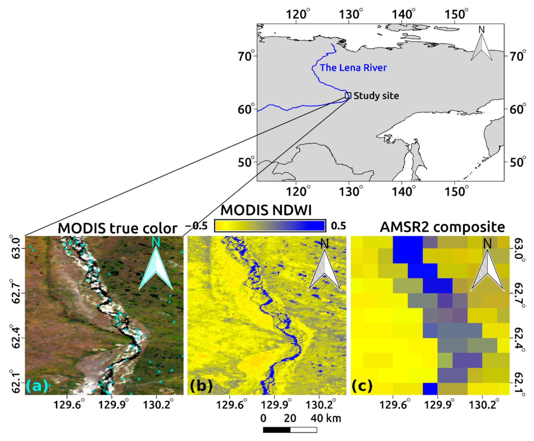
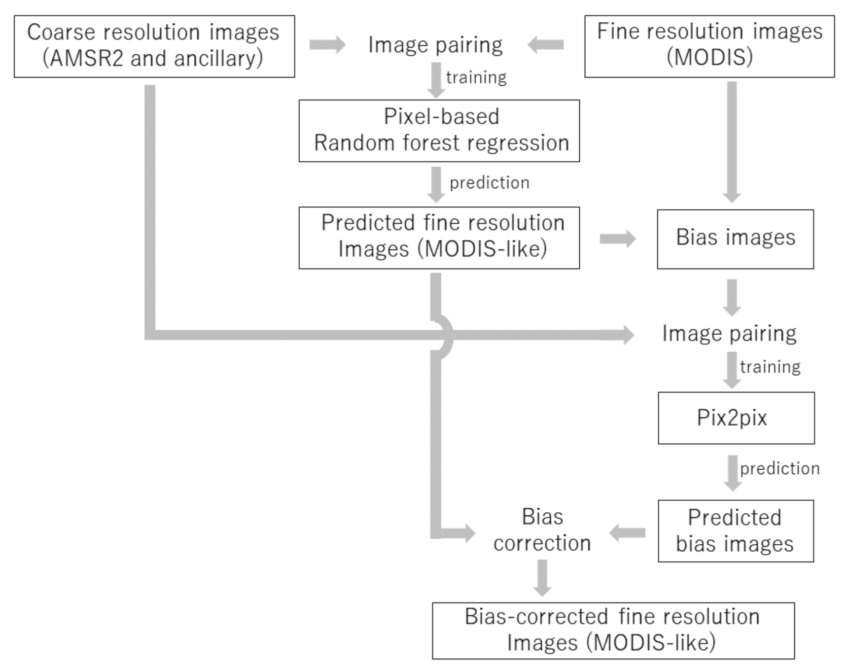
Therefore, we have aimed for data fusion between microwave and optical sensors by combining popular (i.e., random forest) and sophisticated (i.e., pix2pix) ML approaches to obtain open water maps that effectively show subarctic thermokarst lakes with daily frequency. For microwave and optical data, we selected the Advanced Microwave Scanning Radiometer 2 (AMSR2) and Moderate Resolution Imaging Spectroradiometer (MODIS) sensors. AMSR2, which yields passive microwave data, is characterized by a wide swath and high observational frequency (daily), cloud-penetration ability, and coarse spatial resolution (from several to several tens of kilometers, owing to the long microwave wavelength). In contrast, MODIS, which yields optical data, has better spatial resolution (500 m) and is characterized by a relatively low chance (less than daily) of observation of the ground surface owing to cloud interference. Such contrasting features motivated us to apply data fusion between these sets [30].
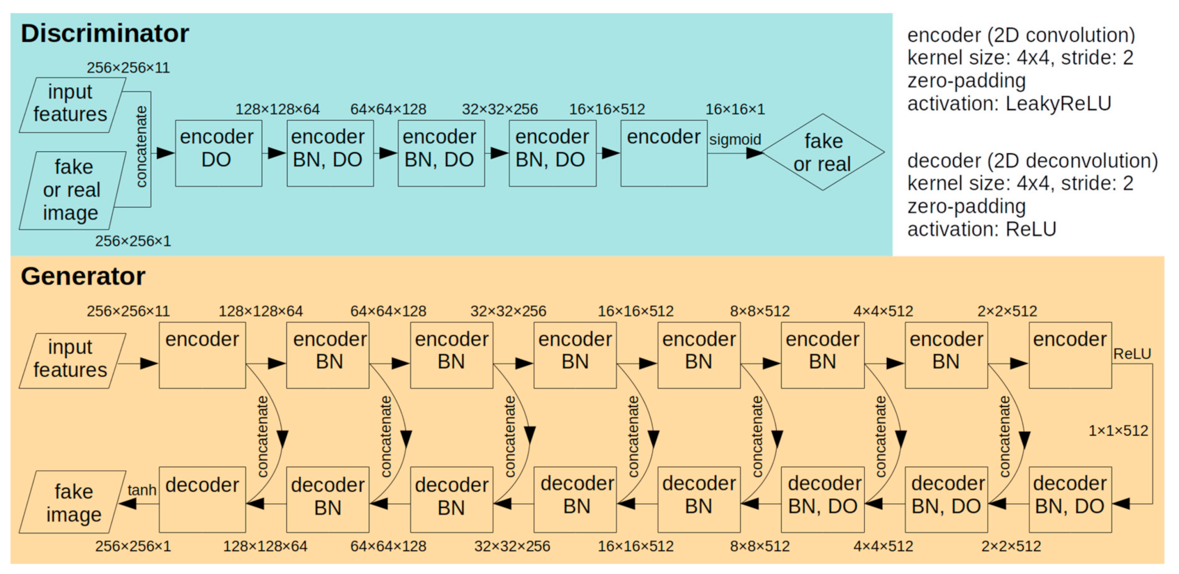
The pix2pix method involves a type of conditional generative adversarial network (GAN) that interfaces two deep CNNs (generator and discriminator [31]) and enables image-to-image translation [32]. Applications of GAN-based image classification [33], segmentation [34], and super-resolution optical imagery [35] have emerged in the remote sensing community. However, owing to the computational cost and nontrivial setup, the application of this technique for monitoring boreal surface water has been barely explored [3]. The novelty of our research is that it addresses the apparent gap between such applications of state-of-the-art ML methods from computer science and spatiotemporal data fusion for satellite remote sensing. Through several experiments (including the timing of the water-index thresholding and input-feature selections), we also aim to provide practical knowledge for the application of sophisticated ML to surface water monitoring.

2. Materials and Methods

2.1. Study Site and Period

We selected Yakutsk (62°:01′–63°:05′ N; 129°:19′–130°:23′ E) in eastern Siberia, which has underlying continuous permafrost, as the study site (Figure 1). The area included the Lena River, which plays an important role in the freshwater supply to the Arctic Ocean [5,36], thermokarst lakes (i.e., open water) created by permafrost thawing [37,38], and a boreal forest (taiga) dominated by larch trees [39]. The surface water extent in this region can vary according to river runoff (primarily controlled by springtime snowmelt [5,6,40]) and both seasonal and interannual fluctuation of thermokarst lakes.
Satellite data were collected from 3 July 2012 (i.e., the beginning of AMSR2 provision) to 2018. This research focused on the detection of liquid surface water; therefore, we excluded the winter season (November–April), when surface water freezes and much of the ground is covered in snow.

2.2. Data and Preprocessing

2.2.1. Advanced Microwave Scanning Radiometer 2

The AMSR2 sensor aboard the Global Change Observation Mission—Water (GCOM-W1) spacecraft is a passive microwave sensor that observes microwave emissions from the Earth’s surface at seven frequency bands (6.925–89.0 GHz) for both horizontal and vertical polarizations. The original spatial resolution (i.e., instantaneous field of view) ranges from several to several tens of kilometers, depending upon the wavebands [41]. We downloaded the Level-3 brightness temperature product from the Japan Aerospace Exploration Agency’s G-Portal website [42]. The data are provided in equidistant cylindrical (latitude–longitude) projection with 0.1° pixel spacing. AMSR2 utilizes microwave wavebands, therefore it is much less affected by clouds than MODIS, and thus no cloud screening was applied. Uncertainty in the brightness temperature is assured by the data provider to within ±1.5 K.
To match the daytime MODIS observation data, only ascending data (recorded at ~13:30 h in local time) were extracted daily. To distinguish the surface water signal from the original brightness temperature, the frequency bands at 18.7, 36.5, and 89.0 GHz were used to calculate several water indices (see Section 2.2.4).

2.2.2. Moderate Resolution Imaging Spectroradiometer

The MODIS aboard the Aqua satellite is an optical sensor that observes radiance in 36 solar-reflective bands; unlike the other MODIS aboard the Terra satellite, only the Aqua MODIS could be used to match the overpass time (~13:30 h in local time) with ascending AMSR2. All surface-reflectance data (MYD09GA) during the study period for two sinusoidal tiles (h23v02 and h24v02) were downloaded from the Land Processes Distributed Active Archive Center data pool [43], mosaicked, and resampled by the nearest-neighbor method on a lat–long projection using the HDF-EOS-to-GeoTIFF-conversion tool. The spatial resolution was 500 m and the temporal resolution was daily, although in practice, ground surface observation was less than daily owing to cloud interference.
Low-quality pixels due to cloud (or cloud-shadow) interception or snow cover were screened by checking the quality assurance data. Geolocation errors may also affect the accuracy of data fusion, particularly when using relatively high-resolution data. The AMSR2 and MODIS images of the study site were well registered to the extent that we visually checked them; however, for the high-resolution data (i.e., MODIS), we also used the phase-only correlation method to ensure co-registration of all images at subpixel scales. During the water extraction process (see Section 2.2.4), we also excluded high-reflectance pixels (more than 0.04 in MODIS band 2) to eliminate any thin cloud or snow that may have unintentionally passed the initial quality check. We confirmed that this treatment did not eliminate surface water pixels and considered it reasonable because waterbodies generally exhibit very low reflectance in the near-infrared spectral region [44].

2.2.3. Ancillary Data

To achieve ML performance, we used day-of-year (DOY) information and the fifth major global reanalysis produced by the European Centre for Medium-Range Weather Forecasts (ERA5-Land) [45] as ancillary inputs when possible. Although ERA5-Land does not produce pure observational data, it includes observational information via a data assimilation scheme, which may be useful in improving ML performance. We selected 17 variables that seemed to explain surface water fluctuation from the ERA5-Land data (Table 1). In addition to the hourly (at UTC 05:00; ~14:00 h in local time) grid-scale variables (i.e., 15 variables from T2M to SWVL4), we prepared accumulated precipitation (during winter in the previous year) and snowmelt (during spring in the current year) data across the entire Lena River basin (TPAGG and SMLTAGG). This is because the snow that accumulates in the previous winter melts during the current spring, affecting river discharge in the region [40].

2.2.4. Water Indices

To enhance the surface water signals from the original satellite data, water indices were calculated for both MODIS and AMSR2.
For the MODIS data, we used the well-known modified normalized-difference water index (NDWI [46]), which is calculated as
NDWI = (GSWIR)/(G + SWIR),
where G is green-surface reflectance (from MODIS band 4) and SWIR is short-wave infrared (MODIS band 7). The pixel-based calculation constructed daily NDWI images derived from MODIS, which can be target images for ML prediction. We also used NDWI to extract the water surface by thresholding NDWI > 0.04 as water. The threshold was determined through visual interpretation at random sampling points across the study site on Google Earth, with the help of a September 2019 field survey, for a total of 100 water pixels thus obtained (Figure 1a).
Compared to optical sensors, there is less consensus concerning a robust index for extracting surface water from passive microwave images. Several researchers have used brightness temperatures associated with different polarizations [47,48] or different frequencies [49,50], which capture the signal from changes in emissivity where surface water exists. Herein, we attempted the use of the normalized difference polarization index (NDPI [48]), fraction of water surface (FWS [49]) estimated by frequency (18.7 GHz and 36.5 GHz), and the basin water index (BWI [50]), which are defined as follows:
N D P I = T B 36.5 , V T B 36.5 , H T B 36.5 , V + T B 36.5 , H
F W S F , V = e F , V e d r y e w e t e d r y ,
e F , V = T B F , V t × T a u T a d t × T s T a d
T s = T B F , V a × T B F , H 1 b a × t × T a d 1 a × T a u b × t ,
B W I = β 0 T B 36.5 , V T B 18.7 , V + β 1 T B 89.0 , V T B 36.5 , V ,
where TBF, P, and eF, P denote the brightness temperature and emissivity at frequency F and polarization P (H: horizontal or V: vertical), respectively; edry and ewet are the emissivities of dry and wet surfaces, respectively; t is the atmospheric transmissivity; Tau and Tad are the upward and downward atmospheric contributions to microwave emission, respectively; Ts is the land-surface temperature; and a, b, β 0 , and β 1 are fitting parameters. Based on the literature review and preliminary parameter tunings for this region, we determined the following: at 18.7 GHz: t = 0.919, Tau = 21.5, Tad = 24.0, a = 0.562, b = 0.434, edry = 0.95, and ewet = 0.59; at 36.5 GHz: t = 0.888, Tau = 29.3, Tad = 31.8, a = 0.502, b = 0.484, edry = 0.95, and ewet = 0.66; moreover, β 0 =   −0.553 and β 1 = 0.213.
We checked the feasibility of using the microwave indices (NDPI, FWS18.7,V, FWS36.5,V, and BWI) to extract surface water [51] and found that they were significantly correlated with the water fractions derived from an optical sensor (r = 0.58 for NDPI, r = 0.51 for FWS18.7,V, r = 0.58 for FWS36.5,V, and r = 0.29 for BWI). However, a unique relationship (i.e., simple regression) over the entire study site between any one microwave index and the optical water fraction was difficult to obtain, mainly because it would entail considering the local relationship between these quantities for each pixel. This is why we used pixel-based or CNN-based ML approaches with multiple microwave indices.

2.3. Machine-Learning Algorithms

Our algorithms are based on two different ML approaches, namely: pixel-based prediction of MODIS images by the random forest approach [52] and bias correction of the predicted image by pix2pix. These methods were implemented in the following environment: Python 3.6.9, tensorflow 2.2.0, keras 2.3.0, CUDA 10.1, cuDNN 7.6.4 with NVIDIA GeForce RTX 2070 SUPER on Ubuntu 18.04. The overall goal of the algorithms to predict the MODIS images from the coincident AMSR2 (and ancillary) images (Figure 2).
Initially, we selected matched pairs by searching for high-quality (minimal cloud interference and few erroneous pixels) MODIS images and their coincident low-resolution (AMSR2 and/or ancillary) images, from which we obtained 272 reference pairs. Spatially coarse-resolution images were oversampled into 500 m resolution via bilinear interpolation [53] to match with the resolution of MODIS. In the preliminary investigation, we confirmed that the use of bilinear interpolation instead of simple oversampling (i.e., a nearest-neighbor technique) mitigates the jaggy spatial pattern [30] in the predicted image when using pixel-based data fusion. Each variable was statistically normalized such that it ranged between 0 and 1. Among the reference pairs, we pulled those of highest quality (34 in total) about once a month for validation. The remaining reference pairs were used to train the MLs.
For basic prediction by the MODIS images in the first phase, we used pixel-based random forest regression. Through the preliminary tuning, we determined the optimal number of trees to be 100 and the minimum node size to be 3. The trained random forest could predict MODIS-like images from the low-resolution images, even when the original MODIS was not obtained owing to cloud cover or lack of observation for other reasons. Popular ML methods such as the random forest [28] and support vector machine [54] techniques have been applied for downscaling satellite-driven data and have shown robust performance; however, the predicted maps tended to show lower variation ranges than the original datasets. This feature is often observed in data-fusion approaches, rendering the effective tracking of abrupt changes or extreme phenomena difficult [55,56].
To address this issue, we attempted bias correction of the first-phase results using sophisticated ML (pix2pix) in the second phase. Subtraction of the original MODIS values from the MODIS-like values predicted by the random forest approach created “bias images”, on which the pix2pix method concentrated to correct the first-phase error. This treatment was expected to adjust the MODIS-like values to more realistic ones, particularly when abrupt change is involved.
In pix2pix, a generator called U-Net [57] competes with a CNN-based discriminator in the training process. The generator creates fake target images with reference to the source images, whereas the discriminator tries to distinguish these images from the originals with the help of the source images. From the perspective of spatiotemporal data fusion, the generator can create high-resolution images from coarse-resolution images after successful training. The structures (Figure 3) and hyperparameters (Table 2) of the generator and the discriminator were carefully tuned to balance their performances. The generator and discriminator were alternately trained by optimizing the following objective function [32] with small batches of size 4:
G * = arg   min G   max D L c G A N G , D + λ L L 1 G
L c G A N G , D = E x , y log D x , y + E x , z log 1 D x , G x , z ,
L L 1 G = E x , y , z y G x , z 1
where G and D are the generator and the discriminator, respectively, x denotes coarse-resolution images, y denotes the original fine-resolution images, z denotes random noise, and λ is a tunable parameter, which we set to 20.
Pix2pix includes a convolution layer, therefore it considers spatial patterns adjacent to a pixel of interest and enables spatially smoothed prediction. In exchange, null pixels disturb the prediction for the adjacent pixels. Therefore, we filled null pixels in the reference MODIS images with monthly climatological values for each pixel.

2.4. Experiments

For best-practice optimization of data fusion over the study site, we conducted the following experiments.

2.4.1. Fusion-then-Thresholding vs. Thresholding-then-Fusion

Our goal was to obtain fine-resolution water maps by NDWI thresholding of MODIS images, therefore we used two data-fusion approaches: (1) predict MODIS NDWI images by data fusion, and then apply thresholding to obtain water maps; (2) obtain water maps from the original MODIS NDWI thresholding before data fusion, apply ML by training with the water maps, and directly predict these maps through data fusion. We compared the accuracies (see Section 2.4.3) of the two approaches using the random forest method and then proceeded with the better approach by applying the following process (pix2pix bias correction).

2.4.2. Input-Feature Selection

Input-feature selection (more accurately known as feature-vector selection) is an essential part of ML. Adding a key feature—one that effectively explains the outcome variable and is independent from the other features—improves the ML accuracy. For example, Mizuochi et al. [28] reported that adding DOY and precipitation information may increase the accuracy of data fusion over a seasonal wetland. In contrast, increasing the number of features does not necessarily lead to successful ML, because a greater number of features requires larger training samples and computational time in general (this is known as the curse of dimensionality [58]).
To see how increasing the dimension of the feature vector improves accuracy, we attempted three cases of inputting features into the random forest: (1) only AMSR2-derived features; (2) AMSR2-derived features with seasonal information (as DOY); and (3) AMSR2-derived features, DOY, and ERA5-Land features (Table 3). The total numbers of input features were 4, 6, and 23, respectively. For DOY information, cosine and sine functions were used as features, such that the end of the previous year and the beginning of the current one could be smoothly connected:
D O Y cos = cos   2 π × D O Y 365.25   and   D O Y sin = sin 2 π × D O Y 365.25 .
Furthermore, we selected only key features to reduce the computational cost in the second phase by checking variable importance in the random forest across the water pixels (those used to determine the NDWI threshold). The 10 best features and the image predicted by the random forest method were concatenated and used as input in the pix2pix. With the 11 input features and corresponding bias images (i.e., target image) for 238 reference pairs, pix2pix was trained. Then, pix2pix predicts bias images for all days in the study period, which were added to corresponding NDWI maps tentatively created by the random forest (i.e., bias correction).
To investigate the dependence of a feature variable upon the other variables, we also investigated variance inflation factors (VIF) of the normalized 23 variables. At 30 points randomly distributed over the entire study site, sample data were collected for each validation day (a total of 34 days) and used for VIF calculation. Unlike traditional multiple-regression analysis, the random forest method has a scheme that randomly extracts feature variables when creating each decision tree and is therefore robust against inter-variance dependence (also known as multicollinearity) to some extent. However, VIF may be helpful for understanding the importance of variables in terms of their independence.

2.4.3. Validation

The water maps derived for validation from the original MODIS and those predicted by ML (or derived from the NDWI predicted by ML) were compared to calculate the overall accuracy (OA), producer’s accuracy (PA), and user’s accuracy (UA). The total water fraction for all available pixels (except null pixels due to cloud cover or other reasons in the original validation map) within the study site was also compared between the original and the predicted water maps, and the mean bias (MB) and root-mean-squared error (RMSE) in the time series were calculated.
The time series for the water fraction derived from the predicted water maps were compared with an independent daily water-fraction dataset with 25 km resolution, namely the Surface Water Microwave Product Series (SWAMPS; v.3 update 1 [59]).
Furthermore, we compared the microwave-intensity maps developed from observations by synthetic-aperture radar (Sentinel 1) to the water maps produced by our algorithm to observe the spatial characteristics of errors in our maps. We obtained backscatter-coefficient (σ0) images (VV polarization, IW mode) acquired in 2017 at a 10 m spatial resolution through the Google Earth engine [60]; because low-σ0 areas are caused by specular reflection over water surfaces, they are useful for detecting surface-water.
Joint Research Centre (JRC) Monthly Water History v1.2 [16] maps were also compared; these classify water/non-water pixels at 30 m resolution for each month using an expert system with Landsat series.

3. Results

3.1. Preliminary Experiments by Random Forest Method

A comparison between the NDWI prediction and the ML-water map (i.e., fusion-then-thresholding vs. thresholding-then-fusion) clearly showed that the former created better water maps for all accuracy criteria and all cases of input data (Table 4). Direct water-map prediction omitted a large proportion of the water pixels, resulting in a large MB, large RMSE, and low PA. Thus, given the current experimental conditions, water maps should not be predicted directly by ML; rather, they should be derived from the NDWI maps predicted in advance by ML.
Based on NDWI map prediction by ML, the best accuracies (PA, UA, and OA) for the water map were obtained using input-features case 3 (83.9%, 85.4%, and 99.4%, respectively). An overall tendency for the addition of more features to create greater accuracy was observed: case 2 (with six features) was superior to case 1 (with four features), and case 3 (with 23 features) was superior to cases 1 and 2. However, the relative MB and RMSE did not always show better results with more features; for example, the relative RMSE in case 3 (40.7%) was better than that in case 2 (41.7%), but the relative MB was not. This may relate to overfitting of the ML model with the limited number of training samples, suggesting a need to reduce the number of input features by selecting key features.
To explore the key features, we investigated variable importance for the 23 possible features in the random forest data (Table 5). The most important feature was DOY (sine and cosine), followed by soil temperature at 7–28 cm depth, microwave indices (NDPI; FWS18.7, V), volumetric soil water at 100–289-cm depth, total evapotranspiration, etc. To avoid overfitting and reduce the computational cost, only the top 10 features (DOYsin and DOYcos; STL2; NDPI; FWS18.7, V; SWVL4; E; FWS36.5, V; STL4; and BWI) were selected for further processing.
The importance of a variable did not necessarily correspond to its independence from the other variables (Table 6). Naturally, some variables exhibited very high VIF values because the properties of the land surface (and microwave indices) are closely interlinked. DOY, E, FWS18.7,V, and SWVL4 were relatively low VIF among the top 10 features, and thus seemed to add values in the ML implementation.
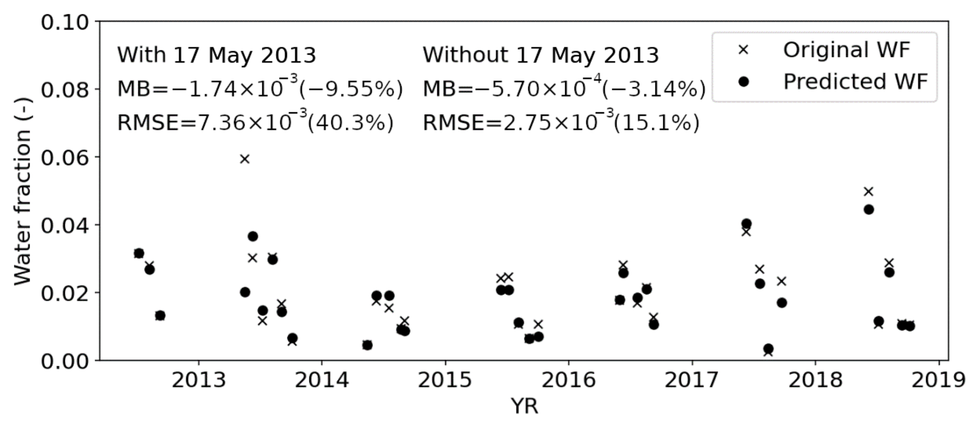
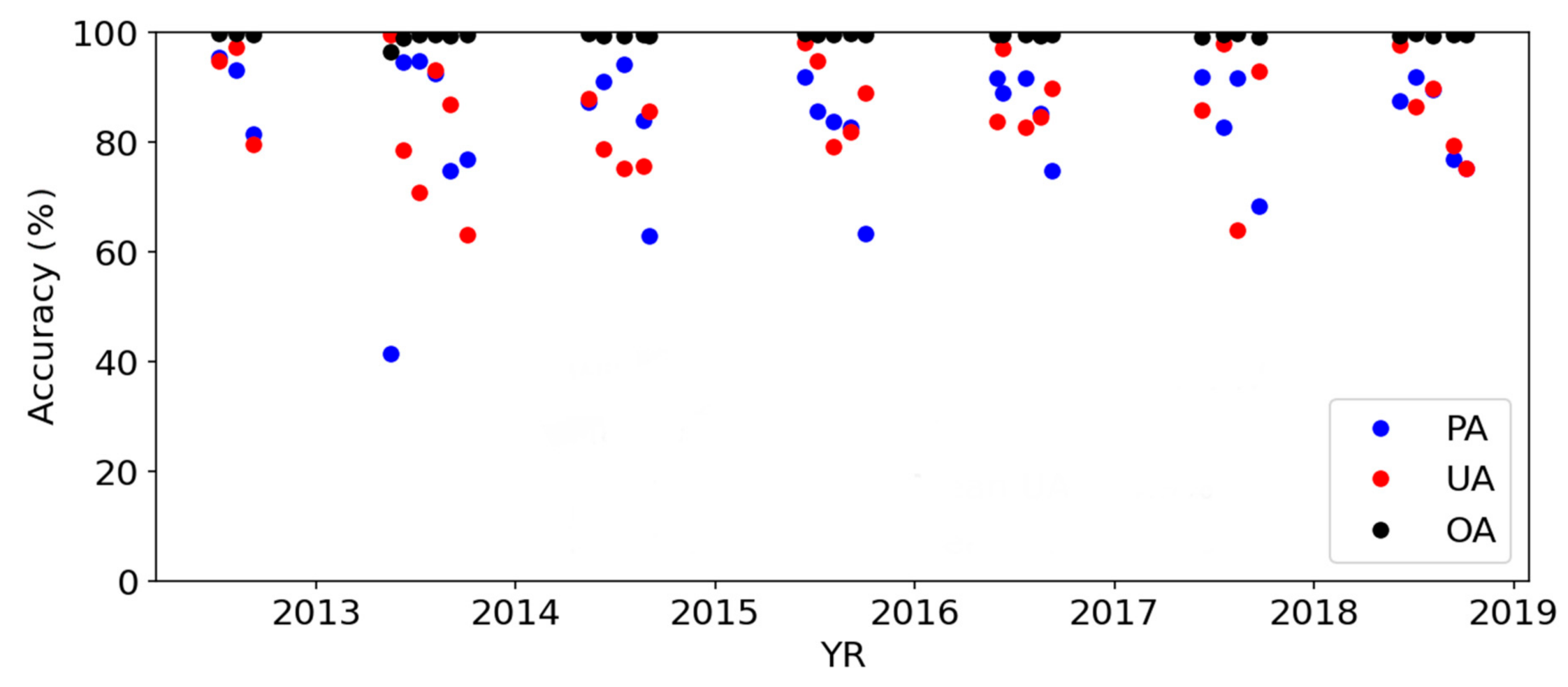
The time-series accuracies of the random forest predictions using the top 10 input features are shown in Figure 4 and Figure 5. Both the relative MB (−9.55%) and RMSE (40.3%) of the total water fraction across the study site were better than those of any cases in the preliminary experiments (Table 4), and the temporal mean PA (83.6%), UA (85.4%), and OA (99.4%) of the water maps (Figure 5) were comparable with those for case 3 (PA = 83.9%, UA = 85.4%, and OA = 99.4%). This confirmed the importance of selecting key features instead of numerous potentially redundant features.
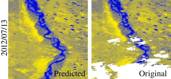
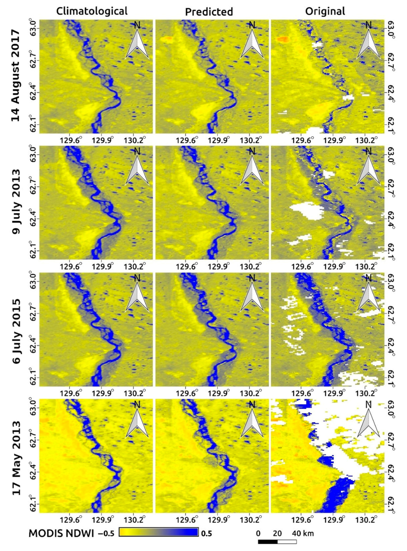
There was an erroneous outlier day (17 May 2013) on which the water fraction was underestimated by ~0.04 and PA was much lower (i.e., large omission of water pixels). According to the original NDWI map on the day (Figure 6), it experienced an irregularly large fraction of water surface, probably because of ice-jam flooding in the spring season. Without this outlier, the performance of the first prediction was: relative MB = −3.14% and relative RMSE = 15.1%.
The similarity of monthly climatological and predicted maps (Figure 6) suggests that the seasonal information is the primary control of prediction by the NDWI maps. This is consistent with the fact that DOY was the most important feature in the random forest prediction (Table 5). However, the predicted maps also resembled the original maps (other than the climatological maps), suggesting the importance of secondary features (e.g., STL2; NDPI; FWS18.7, V) for representing fluctuation or interannual change (other than regular seasonal change).

3.2. Overall Performance of the Algorithm

Based on the results of the preliminary experiment, we trained pix2pix using the top 10 input features to predict bias contained in the first prediction result by the random forest method. The best performance of pix2pix was obtained after 21 epochs of training, from which we created bias-corrected NDWI maps. Although it seemed challenging for pix2pix to further improve the well-tuned random forest results with the limited number of training samples, the final accuracy was somewhat improved (p = 0.14 in the squared error) from MB = −9.55% and RMSE = 40.3% to MB = −8.68% and RMSE = 39.1% with the irregular inundation day (17 May 2013), and from MB = −3.14% and RMSE = 15.1% to MB = −2.43% and RMSE = 14.7% without this outlier. This suggests the potential for this sophisticated ML technique to predict more accurate water maps, including irregular events.
The final NDWI maps predicted for all days during the study period are provided as a Supplementary Video (S1). In the original maps, numerous pixels were screened as cloud cover, cloud shadow, or snow, as well as implausibly high NDWI pixels (probably caused by the cloud cover and cloud shadow that survived the screening process). Hence, the data-available pixels across the study site constituted only 30.3% on average over the entire study period. The combination of the random forest and pix2pix methods successfully filled the gaps and corrected the errors for each day, resulting in virtually 100% availability of MODIS data (except for the period during which AMSR2 was unavailable).
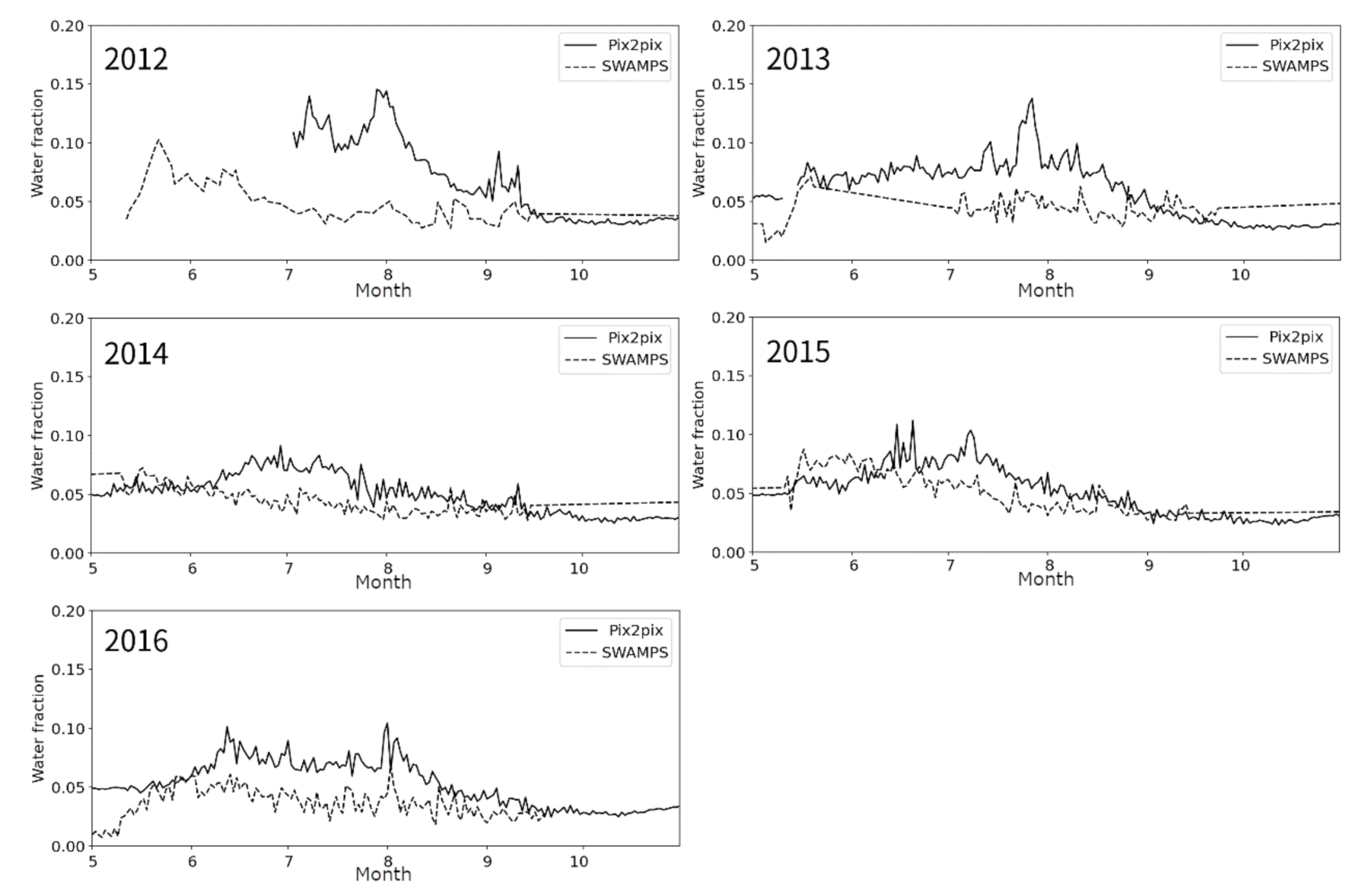
Based on the final predicted NDWI maps, the time series of the water fraction across the study site was estimated via fine-resolution temporal frequency and compared with those from SWAMPS (Figure 7). Seasonal change patterns were generally consistent between them; in particular, both products estimated similar water fractions during the spring and autumn. However, during the summer, our product tended to estimate a larger water fraction. Large discrepancies were observed in 2012 and 2013 in particular.
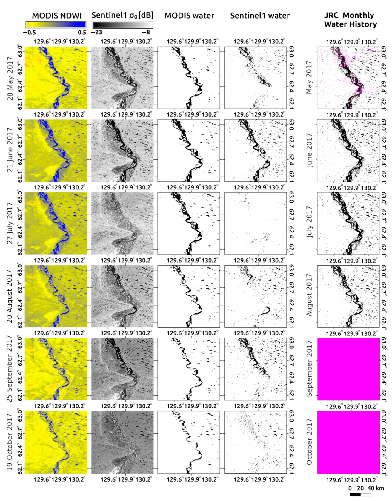
Table 1 and Landsat show several different surface water observation characteristics from our maps (Figure 8). For instance, Sentinel 1 and Landsat (i.e., JRC maps) could observe small-scale thermokarst lakes, particularly along the right bank of the Lena River because of their superior spatial resolutions. In contrast, MODIS is likely to omit sub-grid-scale (< 500 m) thermokarst lakes.
Sentinel 1 also is relatively unstable in automated surface water extraction, because the backscatter coefficient is affected by various factors, such as roughness across waters’ surface due to wind, the existence of vegetation, and the incidence angle. Accordingly, we tentatively determined that σ0 < −20.5 dB indicated water, based on visual interpretation. Hence, a large proportion of the surface water along the Lena River and some thermokarst lakes were omitted by thresholding (particularly on 27 July 2017 and 20 August 2017). Based on our visual interpretation of the raw σ0 images, the surface water extent of the Lena River apparently does not tend to reflect dynamic seasonal change. In contrast, MODIS-based water maps showed continuous seasonal changes characterized by a seasonal increase in the water extent in spring to summer and a seasonal decrease in summer to autumn. The seasonal decrease in surface water extent from July to August was also confirmed in the Landsat-based product, implying consistency between the results obtained from optical sensors.
Sentinel 1 can also easily distinguish frozen river surfaces from liquid water (e.g., on 19 October 2017), whereas MODIS NDWI could not do so. In the predicted water maps, snow masking could not be applied because of the lack of original cloud-free data. Hence, in early May and late October, when the water surface is likely to freeze, the predicted maps in the absence of snow masking may overestimate surface water. Excluding those differences inevitably arising from the sensor features, MODIS and Sentinel 1 created consistent water maps for relatively large-scale water surfaces (21 June 2017).
Our algorithm created wall-to-wall water maps on a daily basis, whereas JRC maps contain no-data pixels even on a monthly basis, probably because of fewer observation opportunities by Landsat, cloud interruption, and error in the scan-line corrector in Landsat 7 (shown as a stripe no-data pattern in May).

4. Discussion

A combination of the random forest and sophisticated (i.e., pix2pix) ML methods created gap-filled MODIS-like water maps with MB = −2.43% and RMSE = 14.7% (excluding the irregular inundation event). Given that the original MODIS dataset was available for only 30.3% of the study period, the substantial improvement in the observation frequency is clearly useful for detailed monitoring of seasonal changes in surface water, particularly during key phenological periods such as foliation and defoliation, river-runoff increase, seasonal permafrost thawing and snow melting, and freezing. The improved temporal frequency enabled wall-to-wall water maps without any no-data pixels to be provided, as compared to the existing JRC water map [16].
Our preliminary experiments revealed that ML prediction of the NDWI maps followed by thresholding created more accurate water maps than those derived solely from direct ML prediction. Similar to previous research reporting that index maps directly predicted by data fusion were more accurate than those calculated from the reflectance predicted by data fusion (i.e., “index-then-blend” was found to be better than “blend-then-index” [61]), we also confirmed the robustness of the index-based approach in terms of different aspects of the data-fusion application. The index-based approach can also provide other options, such as flexible post-tuning of the water threshold, depending upon the location or satellite scenes [62], or relating the index to other hydrological parameters.
The preliminary experiments also revealed that the use of key features in addition to the AMSR2-drived indices improved fusion accuracy. The original 23 input variables closely depend on one another (Table 6), and some are likely to have duplicated information for ML. High VIF does not necessarily mean that the variable in the ML is of lower importance; however, it may be used as an indicator to omit some redundant variables. Principal component analysis is also promising to make the input variables independent from each other. As previous research has reported [28], DOY information clearly helped to describe seasonality (Figure 6; Table 5), which may be primarily important in characterizing variations in the river and thermokarst lakes associated with the annual cycles of snow (accumulation/melting), water (freezing/melting/ice jamming), and the active permafrost layer (freezing/thawing). However, AMSR2-derived indices (e.g., NDPI and FWS18.7, V) are still necessary for tracking interannual variation and sub-seasonal-scale fluctuation, apart from the regular seasonal cycles. Some meteorological parameters, such as soil temperature at 7–28-cm depth (STL2), volumetric soil water at 100–289-cm depth (SWVL4), and total evapotranspiration (E) are also important ancillary data. The soil layers of STL2 and SWVL4 (deeper part of the active layer) may be more important than the others because of the sensitivity of those layers to the hydrological and thermal features of the land surface and the active layer in this region; however, confirming this would require further site-scale investigation.
Contrary to expectations, snowpack in the previous winter and snowmelt in the spring across the basin [40] were not very useful for predictive purposes (Table 5). This is likely due to the spatiotemporal aggregation of those data across very large areas (~2,400,000 km2 of the entire Lena basin and over several months), suggesting the importance of selecting suitable spatiotemporal scales for input features during the data fusion stage. Furthermore, unlike previous research [28], the total precipitation was found to be a variable of lower importance, which can be partly attributed to the fact that the reference high-quality MODIS data were inevitably collected from clear-sky days, upon which the rainfall and snowfall were unlikely to be observed (the so-called clear-sky bias). High-resolution microwave data (i.e., synthetic-aperture radar (SAR), such as Sentinel 1 and the Phased Array-type L-band Synthetic Aperture Radar (PALSAR) series) can be promising alternatives to optical data, because they are less affected by cloud cover, although there are less historical SAR data than optical data.
Our water maps tended to estimate a greater water fraction than SWAMPS across the study site, particularly during the summer. SWAMPS provides the water fraction at a relatively coarse (25 km) resolution on the basis of unmixing of the passive microwave data (the Special Sensor Microwave/Imager; the Special Sensor Microwave Imager Sounder) [59], and because it does not focus on local mapping in Siberia, it may omit sub-grid-scale surface water and seasonal changes of the Lena River. Our achieved 500 m resolution enabled extraction of not only the Lena River but also thermokarst lakes (Figure 6) to some extent. The contrasting density of the thermokarst lakes between the right (1–5%) and the left (0–1%) banks of the Lena River [63,64] was consistently depicted by our water maps (e.g., right bank: 2.4%, left bank: 0.1% in the temporal mean water fraction), thus supporting the validity of our water maps.
Given the progress in producing high-resolution water maps [15,16], our water maps should be further downscaled in conjunction with high-resolution data archives (e.g., Landsat series [56]) to extract small-scale surface water data [3], given that the small-scale thermokarst lakes constitute a nonnegligible proportion of the surface water in the region [65]. The omission of more detailed surface water was indeed observed by comparison between our result and Sentinel 1 (Figure 8). The same comparison also revealed that water extraction by MODIS NDWI was more robust than that derived from the simple thresholding of the VV-polarized backscatter signal of C-band SAR. In contrast, freezing and vegetation cover mixed in with the surface water is also likely to affect NDWI, helping to explain the discrepancy in seasonal changes between the MODIS and Sentinel 1 data. Utilizing SAR’s ability to penetrate vegetation cover and distinguish liquid water from the frozen surface may improve the data-fusion accuracy in creating water maps.
Expansion of the study period using other historical passive microwave data (e.g., AMSR and AMSR-E) is also important for future work. Watts et al. [8] reported a trend of increasing water fraction across wide areas of the subarctic covered by continuous permafrost, as shown by AMSR-E for the period 2003–2010, whereas our more recent water maps (2013–2018) did not exhibit such a trend according to the Mann–Kendall test, neither in the annual mean nor maximum water fractions across the study site. Creating long data records by expanding our analysis to both the past and the future will provide an in-depth understanding of the surface water dynamics of the region due to climate change.
The sophisticated ML (i.e., pix2pix) showed the potential to create more accurate water maps that include irregular events such as ice-jam inundation in the spring season. Although the setup and tuning of such ML techniques can be laborious [3], they are worth applying to address difficult mapping tasks. Expanding the study period may also contribute to obtaining more matched pairs for the ML training, resulting in a more accurate prediction.

5. Conclusions

Our research provides a dynamic water map with a daily frequency and a moderate (500 m) spatial resolution encompassing the heterogeneous thermokarst landscapes in eastern Siberia. The combination of the random forest and pix2pix ML methods has allowed MODIS-like water maps to be predicted from the coincident AMSR2 and ancillary maps. Preliminary random forest experiments demonstrated that post-thresholding of the NDWI maps predicted by ML was better than pre-thresholding for directly predicting water maps. We have shown that adding DOY and reanalysis data as ancillary information may improve the ML prediction accuracy, particularly when describing seasonality. The random forest prediction using 10 key variables was further corrected by the conditional GAN (pix2pix), obtaining a relative mean bias of −2.43% and a relative RMSE of 14.7% in the water fraction across the study site. The generated water maps apparently describe regional seasonality better than SWAMPS independent global water-fraction data, and successfully describe the contrasting distributions of thermokarst lakes between banks of the Lena River. Expansion of the analysis using other historical data sources such as AMSR and AMSR-E, and using high-resolution data sources such as the Landsat, Sentinel, and PALSAR series, will provide further opportunities to understand the long-term surface water dynamics across the site resulting from continuing climate change.

Supplementary Materials

The following are available online at https://0-www-mdpi-com.brum.beds.ac.uk/2072-4292/13/2/175/s1, Video S1: Time series of the predicted and the original NDWI maps.

Author Contributions

Conceptualization, H.M., Y.I., H.N., A.K. and T.H.; methodology, H.M.; software, H.M.; validation, H.M. and Y.I.; formal analysis, H.M.; investigation, H.M. and A.K; data curation, H.M.; writing—original draft preparation, H.M.; writing—review and editing, Y.I., H.N., A.K. and T.H.; visualization, H.M.; project administration, Y.I. and T.H.; funding acquisition, T.H. All authors have read and agreed to the published version of the manuscript.

Funding

This research was supported by JSPS KAKENHI: 19H05668 (Pan-Arctic Water–Carbon Cycles).

Institutional Review Board Statement

Not applicable.

Informed Consent Statement

Not applicable.

Data Availability Statement

Publicly available datasets were analyzed in this study. The data can be found at: AMSR2, https://gportal.jaxa.jp; MODIS: https://e4ftl01.cr.usgs.gov/MOLA; SWAMPS, http://iridl.ldeo.columbia.edu/SOURCES/.NASA/.JPL/.wetlands/dailyinundation/; Sentinel 1 and JRC, https://earthengine.google.com/.

Acknowledgments

The authors appreciate all members of Pan-Arctic Water–Carbon Cycles for research discussion, and Institute for Biological Problems of Cryolithozone Siberian Branch of RAS (IBPC) as a counterpart for the field survey. We also thank Remote Sensing Group members in the Geological Survey of Japan (GSJ), National Institute of Advanced Industrial Science and Technology (AIST) for the discussion on satellite data processing.

Conflicts of Interest

The authors declare no conflict of interest.

References

  1. Snow, Water, Ice and Permafrost in the Arctic (SWIPA) 2017; Arctic Monitoring and Assessment Programme (AMAP): Oslo, Norway, 2017; p. 269. Available online: https://swipa.amap.no/ (accessed on 4 January 2021).
  2. Suzuki, K.; Matuo, M. Remote sening of Terrestrial Water. In Water-Carbon Dynamics in Eastern Siberia, 1st ed.; Ohta, T., Hiyama, T., Iijima, Y., Kotani, A., Maximov, T.C., Eds.; Springer Nature: Singapore, 2019; pp. 253–277. [Google Scholar]
  3. Chasmer, L.; Mahoney, C.; Millard, K.; Nelson, K.; Peters, D.L.; Merchant, M.A.; Hopkinson, C.; Brisco, B.; Niemann, K.O.; Montgomery, J.; et al. Remote Sensing of Boreal Wetlands 2: Methods for Evaluating Boreal Wetland Ecosystem State and Drivers of Change. Remote Sens. 2020, 12, 1321. [Google Scholar] [CrossRef] [Green Version]
  4. Velicogna, I.; Tong, J.; Zhang, T.; Kimball, J.S. Increasing subsurface water storage in discontinuous permafrost areas of the Lena River basin, Eurasia, detected from GRACE. Geophys. Res. Lett. 2012, 39, 09403. [Google Scholar] [CrossRef] [Green Version]
  5. Suzuki, K.; Hiyama, T.; Matsuo, K.; Ichii, K.; Iijima, Y.; Yamazaki, D. Accelerated continental-scale snowmelt and ecohydrological impacts in the four largest Siberian river basins in response to spring warming. Hydrol. Process. 2020, 34, 3867–3881. [Google Scholar] [CrossRef]
  6. Yang, D.; Zhao, Y.; Armstrong, R.; Robinson, D.; Brodzik, M.-J. Streamflow response to seasonal snow cover mass changes over large Siberian watersheds. J. Geophys. Res. Space Phys. 2007, 112, F02S22. [Google Scholar] [CrossRef] [Green Version]
  7. Bartsch, A.; Balzter, H.; George, C. The influence of regional surface soil moisture anomalies on forest fires in Siberia observed from satellites. Environ. Res. Lett. 2009, 4, 045021. [Google Scholar] [CrossRef] [Green Version]
  8. Watts, J.D.; Kimball, J.S.; Jones, L.A.; Schroeder, R.; McDonald, K.C. Satellite Microwave remote sensing of contrasting surface water inundation changes within the Arctic–Boreal Region. Remote Sens. Environ. 2012, 127, 223–236. [Google Scholar] [CrossRef]
  9. Guimberteau, M.; Zhu, D.; Maignan, F.; Huang, Y.; Yue, C.; Dantec-Nédélec, S.; Ottlé, C.; Jornet-Puig, A.; Bastos, A.; Laurent, P.; et al. ORCHIDEE-MICT (v8.4.1), a land surface model for the high latitudes: Model description and validation. Geosci. Model Dev. 2018, 11, 121–163. [Google Scholar] [CrossRef] [Green Version]
  10. Hogstrom, E.; Bartsch, A. Impact of Backscatter Variations Over Water Bodies on Coarse-Scale Radar Retrieved Soil Moisture and the Potential of Correcting With Meteorological Data. IEEE Trans. Geosci. Remote Sens. 2016, 55, 3–13. [Google Scholar] [CrossRef]
  11. Cherbunina, M.Y.; Shmelev, D.G.; Brouchkov, A.V.; Kazancev, V.S.; Argunov, R.N. Patterns of spatial methane distribution in the upper layers of the permafrost in central Yakutia. Moskow Univ. Geol. Bull. 2018, 73, 100–108. [Google Scholar] [CrossRef]
  12. Lehner, B.; Döll, P. Development and validation of a global database of lakes, reservoirs and wetlands. J. Hydrol. 2004, 296, 1–22. [Google Scholar] [CrossRef]
  13. Prigent, C.; Matthews, E.; Aires, F.; Rossow, W.B. Remote sensing of global wetland dynamics with multiple satellite data sets. Geophys. Res. Lett. 2001, 28, 4631–4634. [Google Scholar] [CrossRef] [Green Version]
  14. Fluet-Chouinard, E.; Lehner, B.; Rebelo, L.-M.; Papa, F.; Hamilton, S.K. Development of a global inundation map at high spatial resolution from topographic downscaling of coarse-scale remote sensing data. Remote Sens. Environ. 2015, 158, 348–361. [Google Scholar] [CrossRef]
  15. Yamazaki, D.; Trigg, M.A.; Ikeshima, D. Development of a global ~90 m water body map using multi-temporal Landsat images. Remote Sens. Environ. 2015, 171, 337–351. [Google Scholar] [CrossRef]
  16. Pekel, J.-F.; Cottam, A.; Gorelick, N.; Belward, A.S. High-resolution mapping of global surface water and its long-term changes. Nature 2016, 540, 418–422. [Google Scholar] [CrossRef]
  17. Zhu, X.; Chen, J.; Gao, F.; Chen, X.; Masek, J.G. An enhanced spatial and temporal adaptive reflectance fusion model for complex heterogeneous regions. Remote Sens. Environ. 2010, 114, 2610–2623. [Google Scholar] [CrossRef]
  18. Curzi, G.; Modenini, D.; Tortora, P. Large constellations of small sateliites: A survey of near future challenges and missions. Aerospace 2020, 7, 133. [Google Scholar] [CrossRef]
  19. Houborg, R.; McCabe, M.F. A cubesat enabled spatio-temporal enhancement method (CESTEM) utilizing Planet, Landsat and MODIS data. Remote Sens. Environ. 2018, 209, 211–226. [Google Scholar] [CrossRef]
  20. Chen, B.; Huang, B.; Xu, B. Comparison of spatiotemporal fusion models: A review. Remote Sens. 2015, 7, 1798–1835. [Google Scholar] [CrossRef] [Green Version]
  21. Belgiu, M.; Stein, A. Spatiotemporal image fusion in remote sensing. Remote Sens. 2019, 11, 818. [Google Scholar] [CrossRef] [Green Version]
  22. Gao, F.; Masek, J.; Schwaller, M.; Hall, F. On the blending of the Landsat and MODIS surface reflectance: Predicting daily Landsat surface reflectance. IEEE Trans. Geosci. Remote Sens. 2006, 44, 2207–2218. [Google Scholar]
  23. Roy, D.P.; Ju, J.; Lewis, P.; Schaaf, C.; Gao, F.; Hansen, M.; Lindquist, E. Multi-temporal MODIS-Landsat data fusion for relative radiometric normalization, gap filling, and prediction of Landsat data. Remote Sens. Environ. 2008, 112, 3112–3130. [Google Scholar] [CrossRef]
  24. Cammalleri, C.; Anderson, M.C.; Gao, F.; Hain, C.R.; Kustas, W.P. Mapping daily evapotranspiration at field scales over rainfed and irrigated agricultural areas using remote sensing data fusion. Agric. For. Meteorol. 2014, 186, 1–11. [Google Scholar] [CrossRef] [Green Version]
  25. Weng, Q.; Fu, P.; Gao, F. Generating daily land surface temperature at Landsat resolution by fusing Landsat and MODIS data. Remote Sens. Environ. 2014, 145, 55–67. [Google Scholar] [CrossRef]
  26. Houborg, R.; McCabe, M.S.; Gao, F. A Spatio-Temporal Enhancement Method for medium resolution LAI (STEM-LAI). Int. J. Appl. Earth Obs. Geoinf. 2016, 47, 15–29. [Google Scholar] [CrossRef] [Green Version]
  27. Li, X.; Long, D. An improvement in accuracy and spatiotemporal continuity of the MODIS precipitable water vapor product based on a data fusion approach. Remote Sens. Environ. 2020, 248, 111966. [Google Scholar] [CrossRef]
  28. Mizuochi, H.; Nishiyama, C.; Ridwansyah, I.; Nasahara, K.N. Monitoring of an Indonesian tropical wetland by machine learning-based data fusion of passive and active microwave sensors. Remote Sens. 2018, 10, 1235. [Google Scholar] [CrossRef] [Green Version]
  29. Sahour, H.; Sultan, M.; Vazifedan, M.; Abdelmohsen, K.; Karki, S.; Yellich, J.A.; Gebremichael, E.; Alshehri, F.; Elbayoumi, T.M. Statistical applications to downscale GRACE-derived terrestrial water storage data and to fill temporal gaps. Remote Sens. 2020, 12, 533. [Google Scholar] [CrossRef] [Green Version]
  30. Mizuochi, H.; Hiyama, T.; Ohta, T.; Nasahara, K.N. Evaluation of the surface water distribution in north-central Namibia based on MODIS and AMSR series. Remote Sens. 2014, 6, 7660–7682. [Google Scholar] [CrossRef] [Green Version]
  31. Mirza, M.; Osindero, S. Conditional generative adversarial nets. arXiv 2014, arXiv:1411.1784. [Google Scholar]
  32. Isola, P.; Zhu, J.-Y.; Zhou, T.; Efros, A.A. Image-to-image translation with conditional adversarial networks. In Proceedings of the 2017 IEEE Conference on Computer Vision and Pattern Recognition (CVPR), Honolulu, HI, USA, 21–26 July 2017; pp. 5967–5976. [Google Scholar]
  33. Wang, X.; Yan, H.; Huo, C.; Yu, J.; Pant, C. Enhancing pix2pix for remote sensing image classification. In Proceedings of the 24th International Conference on Pattern Recognition (ICPR), Beijing, China, 20–24 August 2018; pp. 2332–2336. [Google Scholar] [CrossRef]
  34. Kniaz, V.V. Conditional GANs for semantic segmentation of multispectral satellite images. In Proceedings of the SPIE 10789, Image and Signal Processing for Remote Sensing XXIV, Berlin, Germany, 10–12 September 2018. [Google Scholar]
  35. Xiong, Y.; Guo, S.; Chen, J.; Deng, X.; Sun, L.; Zheng, X.; Xu, W. Improved SRGAN for remote sensing image super-resolution across locations and sensors. Remote Sens. 2020, 12, 1263. [Google Scholar] [CrossRef] [Green Version]
  36. Costard, F.; Gautier, E.; Brunstein, D.; Hammadi, J.; Fedorov, A.; Yang, D.; Dupeyrat, L. Impact of the global warming on the fluvial thermal erosion over the Lena River in Central Siberia. Geophys. Res. Lett. 2007, 34, 14501. [Google Scholar] [CrossRef]
  37. Kirpotin, S.; Polishchuk, Y.; Bryksina, N. Abrupt changes of thermokarst lakes in Western Siberia: Impacts of climatic warming on permafrost melting. Int. J. Environ. Stud. 2009, 66, 423–431. [Google Scholar] [CrossRef]
  38. Katamura, F.; Fukuda, M.; Bosikov, N.P.; Desyatkin, R.V.; Nakamura, T.; Moriizumi, J. Thermokarst formation and vegetation dynamics inferred from a palynological study in Central Yakutia, Eastern Siberia, Russia. Arct. Antarct. Alp. Res. 2006, 38, 561–570. [Google Scholar] [CrossRef] [Green Version]
  39. Osawa, A.; Zyryanova, O.A.; Matsuura, Y.; Kajimoto, T.; Wein, R.W. (Eds.) Permafrost Ecosystems—Siberian Larch Forests, Ecological Studies; Springer: London, UK, 2010; Volume 2019, pp. 3–15. [Google Scholar]
  40. Oshima, K.; Tachibana, Y.; Hiyama, T. Climate and year-to-year variability of atmospheric and terrestrial water cycles in the three great Siberian rivers. J. Geophys. Res. Atmos. 2015, 120, 3043–3062. [Google Scholar] [CrossRef]
  41. GCOM-W1 “SHIZUKU” Data Users Handbook. Japan Aerospace Exploration Agency, January 2013. Available online: https://gportal.jaxa.jp/gpr/assets/mng_upload/GCOM-W/GCOM-W1_SHIZUKU_Data_Users_Handbook_EN.pdf (accessed on 17 December 2020).
  42. JAXA GPortal. Available online: https://gportal.jaxa.jp (accessed on 3 November 2020).
  43. LP DAAC Data pool. Available online: https://e4ftl01.cr.usgs.gov/MOLA (accessed on 3 November 2020).
  44. Petty, G.W. A First Course in Atmospheric Radiation, 2nd ed.; Sundog Publishing: Madison, WI, USA, 2006; p. 100. [Google Scholar]
  45. Hersbach, H.; Bell, B.; Berrisford, P.; Hirahara, S.; Horányi, A.; Muñoz-Sabater, J.; Nicolas, J.; Peubey, C.; Radu, R.; Schepers, D.; et al. The ERA5 global reanalysis. Q. J. R. Meteorol. Soc. 2020, 146, 1999–2049. [Google Scholar] [CrossRef]
  46. Xu, H. Modification of normalized difference water index (NDWI) to enhance open water features in remotely sensed imagery. Int. J. Remote Sens. 2006, 27, 3025–3033. [Google Scholar] [CrossRef]
  47. Sippel, S.J.; Hamilton, S.K.; Melack, J.M.; Choudhury, B.J. Determination of inundation area in the Amazon river floodplain using the SMMR 37 GHz polarization difference. Remote Sens. Environ. 1994, 76, 70–76. [Google Scholar] [CrossRef]
  48. Takeuchi, W.; Gonzalez, L. Blending MODIS and AMSR-E to predict daily land surface water coverage. In Proceedings of the International Remote Sensing Symposium (ISRS), Busan, Korea, 29 October 2009. [Google Scholar]
  49. Fily, M.; Royer, A.; Goita, K.; Prigent, C. A simple retrieval method for land surface temperature and fraction of water surface determination from satellite microwave brightness temperatures in sub-arctic areas. Remote Sens. Environ. 2003, 85, 328–338. [Google Scholar] [CrossRef]
  50. Temimi, M.; Leconte, R.; Brissette, F.; Chaouch, N. Flood monitoring over the Mackenzie River Basin using passive microwave data. Remote Sens. Environ. 2005, 98, 344–355. [Google Scholar] [CrossRef]
  51. Mizuochi, H.; Hiyama, T. Investigation of the ability of a passive microwave sensor to monitor surface water over complex landscape in Eastern Siberia. In Proceedings of the IEEE International Geoscience and Remote Sensing Symposium, 26 September–2 October 2020; Available online: https://igarss2020.org/ (accessed on 4 January 2021).
  52. Breiman, L. Random forests. Mach. Learn. 2001, 45, 5–32. [Google Scholar] [CrossRef] [Green Version]
  53. Huang, B.; Song, H. Spatiotemporal Reflectance Fusion via Sparse Representation. IEEE Trans. Geosci. Remote. Sens. 2012, 50, 3707–3716. [Google Scholar] [CrossRef]
  54. Ichii, K.; Ueyama, M.; Kondo, M.; Saigusa, N.; Kim, J.; Alberto, M.C.; Ardö, J.; Euskirchen, E.S.; Kang, M.; Hirano, T.; et al. New data-driven estimation of terrestrial CO2 fluxes in Asia using a standardized database of eddy covariance measurements, remote sensing data, and support vector regression. J. Geophys. Res. Biogeosci. 2017, 122, 767–795. [Google Scholar] [CrossRef]
  55. Hilker, T.; Wulder, M.A.; Coops, N.C.; Linke, J.; McDermid, G.; Masek, J.G.; Gao, F.; White, J.C. A new data fusion model for high spatial- and temporal-resolution mapping of forest disturbance based on Landsat and MODIS. Remote Sens. Environ. 2009, 113, 1613–1627. [Google Scholar] [CrossRef]
  56. Mizuochi, H.; Hiyama, T.; Ohta, T.; Fujioka, Y.; Kambatuku, J.R.; Iijima, M.; Nasahara, K.N. Development and evaluation of a lookup-table-based approach to data fusion for seasonal wetlands monitoring: An integrated use of AMSR series, MODIS, and Landsat. Remote Sens. Environ. 2017, 199, 370–388. [Google Scholar] [CrossRef]
  57. Ronneberger, O.; Fischer, P.; Brox, T. U-Net: Convolutional networks for biomedical image segmentation. arXiv 2015, arXiv:1505.04597. [Google Scholar]
  58. Bishop, C.M. Pattern Recognition and Machine Learning; Springer: New York, NY, USA, 2006; pp. 33–38. [Google Scholar]
  59. Schroeder, R.; McDonald, K.C.; Chapman, B.D.; Jensen, K.; Podest, E.; Tessler, Z.D.; Bohn, T.J.; Zimmermann, R. Development and evaluation of a multi-year fractional surface water data set derived from Active/Passive microwave remote sensing data. Remote Sens. 2015, 7, 16688–16732. [Google Scholar] [CrossRef] [Green Version]
  60. Gorelick, N.; Hancher, M.; Dixon, M.; Ilyushchenko, S.; Thau, D.; Moore, R. Google Earth Engine: Planetary-scale geospatial analysis for everyone. Remote Sens. Environ. 2017, 202, 18–27. [Google Scholar] [CrossRef]
  61. Jarihani, A.A.; McVicar, T.R.; Van Niel, T.G.; Emelyanova, I.V.; Callow, J.N.; Johansen, K. Blending Landsat and MODIS data to generate nultispectral indices: A comparison of “index-then-blend” and “blend-then-index” approaches. Remote Sens. 2014, 6, 9213–9238. [Google Scholar] [CrossRef] [Green Version]
  62. Ji, L.; Zhang, L.; Wylie, B. Analysis of dynamic thresholds for the normalized difference water index. Photogramm. Eng. Rem. S. 2009, 75, 1307–1317. [Google Scholar] [CrossRef]
  63. Iijima, Y.; Fedorov, A.N. Permafrost-Forest Dynamics. In Water-Carbon Dynamics in Eastern Siberia, 1st ed.; Ohta, T., Hiyama, T., Iijima, Y., Kotani, A., Maximov, T.C., Eds.; Springer: Singapore, 2019; pp. 175–205. [Google Scholar]
  64. Bosikov, N.P. Evolution of Alases in Central Yakutia; Permafrost Institute, Siverian Division of Russian Academy of Science: Yakutsk, Russia, 1991; p. 127. (In Russian) [Google Scholar]
  65. Saito, H.; Iijima, Y.; Basharin, N.I.; Fedorov, A.N.; Kunitsky, V.V. Thermokarst development detected from high-definition topographic data in central Yakutia. Remote Sens. 2018, 10, 1579. [Google Scholar] [CrossRef] [Green Version]
Figure 1. Study site and corresponding satellite data from 11 September 2016: (a) True-color image of Moderate Resolution Imaging Spectroradiometer (MODIS) with distributed sampling points of water pixels (represented by the blue stars); (b) modified normalized-difference water index (NDWI) derived from MODIS; (c) False-color image derived from the Advanced Microwave Scanning Radiometer 2 (AMSR2) by assigning brightness temperature. Red, 36-GHz horizontal polarization; green, vertical polarization; blue, normalized-difference polarization index.
Remotesensing 13 00175 g001
Figure 2. Overall algorithm for data fusion.
Remotesensing 13 00175 g002
Figure 3. Structures of the generator and the discriminator in the pix2pix method. Spatial features are extracted in the high-dimensional space through the multiple-convolution process. DO: drop-out rate (0.25); BN: batch normalization. The slope of the LeakyReLU activation function was 0.2. The numbers accompanying the elements represent the rows and columns of each image, and dimension in the feature vector. For example, 256 × 256 × 11 denotes 11 feature images that have a 256 × 256 pixel size.
Remotesensing 13 00175 g003
Figure 4. Time-series comparison of total water fraction (WF) for all original available pixels across the study site between the original and predicted maps. Prediction was performed using the random forest method with the top 10 features. The temporal mean bias (MB) and root-mean-squared error (RMSE) are shown with and without the outlier day (17 May 2013).
Remotesensing 13 00175 g004
Figure 5. Time series of producer’s accuracy (PA), user’s accuracy (UA), and overall accuracy (OA) of the water maps derived from the predicted normalized-difference water index (NDWI) maps, in comparison to the original validation maps.
Remotesensing 13 00175 g005
Figure 6. Comparison of normalized-difference water-index (NDWI) maps on four typical days (14 August 2017; 9 July 2013; 6 July 2015; 17 May 2013), which correspond to the minimum, 33-percentile, 66-percentile, and maximum water fractions, respectively, in the original NDWI maps (left column). Monthly climatological NDWI maps derived from time-series of original NDWI maps (center column). NDWI maps predicted by the random-forest method (right column). Original NDWI maps. MODIS: Moderate Resolution Imaging Spectroradiometer. White pixels indicate null values (mainly due to cloud cover)].
Remotesensing 13 00175 g006
Figure 7. Comparison of the time-series water fractions across study sites between our fusion dataset (pix2pix) and the Surface Water Microwave Product Series (SWAMPS) [59] data for the May–October period of 2012–2016. Our data started from 3 July 2012 (per data availability of Advanced Microwave Scanning Radiometer 2 (AMSR2), and SWAMPS product data which ended in 2016).
Remotesensing 13 00175 g007
Figure 8. Comparison of MODIS with Sentinel 1 images for six dates (once per month) during 2017, and with the Joint Research Centre (JRC) Monthly Water History v1.2 in the corresponding month. Columns from left to right: MODIS NDWI maps; Sentinel 1 backscatter coefficient (σ0) maps; MODIS water maps (NDWI > 0.04); Sentinel 1 water maps (σ0 < −20.5); and the JRC maps. Black and white in the water maps correspond to water and non-water pixels, respectively. Magenta indicates no data. For Sentinel 1, the smoothing filter (i.e., spatial averaging within the 11 × 11 window) was applied to reduce noise.
Remotesensing 13 00175 g008
Table 1. Selected ERA5-Land variables as input features for machine learning.
VariablesAbbreviationsUnitsSpatial ResolutionTemporal Resolution
2 m temperatureT2MK0.1° × 0.1°Hourly
Skin reservoir contentSRCm of water equivalent0.1° × 0.1°Hourly
Skin temperatureSKTK0.1° × 0.1°Hourly
SnowmeltSMLTm of water equivalent0.1° × 0.1°Hourly
Soil temperature in layer 1 (0–7 cm)STL1K0.1° × 0.1°Hourly
Soil temperature in layer 2 (7–28 cm)STL2K0.1° × 0.1°Hourly
Soil temperature in layer 3 (28–100 cm)STL3K0.1° × 0.1°Hourly
Soil temperature in layer 4 (100–289 cm)STL4K0.1° × 0.1°Hourly
Surface runoffSROm0.1° × 0.1°Hourly
Total evaporationEm of water equivalent0.1° × 0.1°Hourly
Total precipitationTPm0.1° × 0.1°Hourly
Volumetric soil water in layer 1 (0–7 cm)SWVL1m3/m30.1° × 0.1°Hourly
Volumetric soil water in layer 2 (7–28 cm)SWVL2m3/m30.1° × 0.1°Hourly
Volumetric soil water in layer 3 (28–100 cm)SWVL3m3/m30.1° × 0.1°Hourly
Volumetric soil water in layer 4 (100–289 cm)SWVL4m3/m30.1° × 0.1°Hourly
Basin aggregated total precipitationTPAGGmEntire basinAggregated 1
Basin aggregated snowmeltSMLTAGGm of water equivalentEntire basinAggregated 2
1 Aggregated monthly value from October of the previous year until April of the current year. 2 Aggregated monthly value from March through May of the current year.
Table 2. Hyperparameters in pix2pix.
NameOptimizerBeta 1Beta 2Learning Rate
GeneratorAdam0.50.9990.0004
DiscriminatorAdam0.50.9990.00002
Table 3. Three cases of input features for predicting the MODIS image (abbreviations for ERA5-Land are explained in Table 1). NDPI: normalized difference polarization index, FWS: fraction of water surface, BWI: basin water index, and DOY: day of year.
CaseInput Features
1NDPI; FWS18.7, V; FWS36.5, V; BWI
2NDPI; FWS18.7, V; FWS36.5, V; BWI; DOYcos and DOYsin
3NDPI; FWS18.7, V; FWS36.5, V; BWI; DOYcos and DOYsin; T2M; SRC; SKT; SMLT, STL1, STL2, STL3, STL4; SRO; E; TP; SWVL1, SWVL2, SWVL3, SWVL4; TPAGG; SMLTAGG
Table 4. Temporal mean accuracy comparison among cases of input features and among prediction targets for available pixels across the study site. MB, mean bias of total water fraction; RMSE, root mean squared error; OA, overall accuracy of water maps; PA, producer’s accuracy; UA, user’s accuracy.
Case of Input FeaturesFusion TargetRelative MB (%)Relative RMSE (%)Mean PA (%)Mean UA (%)Mean OA (%)
1NDWI map−10.841.782.683.599.3
2NDWI map−9.5541.783.185.099.4
3NDWI map−9.6340.783.985.499.4
1Water map−10513943.985.598.8
2Water map−86.711848.387.498.9
3Water map−87.311949.288.398.9
Table 5. Variable importance of possible input features in random forest data for water pixels. Features are sorted in descending order of variable importance; abbreviations are explained in Table 1.
RankInput FeaturesVariable ImportanceRankInput FeaturesVariable ImportanceRankInput FeaturesVariable Importance
1DOYsin0.1059STL40.04717SKT0.033
2DOYcos0.09610BWI0.04518TPACC0.022
3STL20.06911SWVL30.04419SMLTACC0.020
4NDPI0.06912SWVL20.04320TP0.008
5FWS18.7, V0.06313STL10.04221SRC0.007
6SWVL40.06014SWVL10.04122SMLT0.003
7E0.05315STL30.04023SRO0.003
8FWS36.5, V0.05216T2M0.036
Table 6. Variance inflation factor (VIF) for possible input features. Lower VIF values represent greater independence from the other variables. Features are sorted in descending order of variable importance shown in Table 5; abbreviations are explained in Table 1.
RankInput FeaturesVIFRankInput FeaturesVIFRankInput FeaturesVIF
7DOYsin23.516STL4173.223SKT3593.0
8DOYcos26.017BWI302.16TPACC14.4
20STL21593.115SWVL3153.95SMLTACC12.3
18NDPI920.512SWVL2127.84TP5.7
10FWS18.7, V81.822STL12921.03SRC4.5
11SWVL490.314SWVL1146.21SMLT1.4
9E51.113STL3135.62SRO1.8
19FWS36.5, V1202.021T2M2172.4
Publisher’s Note: MDPI stays neutral with regard to jurisdictional claims in published maps and institutional affiliations.

