Article

Stacked Autoencoders Driven by Semi-Supervised Learning for Building Extraction from near Infrared Remote Sensing Imagery

by
Eftychios Protopapadakis
*,
Anastasios Doulamis
,
Nikolaos Doulamis
and
Evangelos Maltezos
School of Rural and Surveying Engineering, National Technical University of Athens, 15780 Zografos, Greece
*
Author to whom correspondence should be addressed.
Submission received: 16 December 2020 / Revised: 14 January 2021 / Accepted: 18 January 2021 / Published: 21 January 2021
(This article belongs to the Special Issue Signal and Image Processing for Remote Sensing)

Abstract

:
In this paper, we propose a Stack Auto-encoder (SAE)-Driven and Semi-Supervised (SSL)-Based Deep Neural Network (DNN) to extract buildings from relatively low-cost satellite near infrared images. The novelty of our scheme is that we employ only an extremely small portion of labeled data for training the deep model which constitutes less than 0.08% of the total data. This way, we significantly reduce the manual effort needed to complete an annotation process, and thus the time required for creating a reliable labeled dataset. On the contrary, we apply novel semi-supervised techniques to estimate soft labels (targets) of the vast amount of existing unlabeled data and then we utilize these soft estimates to improve model training. Overall, four SSL schemes are employed, the Anchor Graph, the Safe Semi-Supervised Regression (SAFER), the Squared-loss Mutual Information Regularization (SMIR), and an equal importance Weighted Average of them (WeiAve). To retain only the most meaning information of the input data, labeled and unlabeled ones, we also employ a Stack Autoencoder (SAE) trained under an unsupervised manner. This way, we handle noise in the input signals, attributed to dimensionality redundancy, without sacrificing meaningful information. Experimental results on the benchmarked dataset of Vaihingen city in Germany indicate that our approach outperforms all state-of-the-art methods in the field using the same type of color orthoimages, though the fact that a limited dataset is utilized (10 times less data or better, compared to other approaches), while our performance is close to the one achieved by high expensive and much more precise input information like the one derived from Light Detection and Ranging (LiDAR) sensors. In addition, the proposed approach can be easily expanded to handle any number of classes, including buildings, vegetation, and ground.

Graphical Abstract

1. Introduction

Land cover classification is a widely studied field since the appearance of the first satellite images. In the last two decades, the sensors attached to satellites have evolved in a way that nowadays allow the capture of high-resolution images which may go beyond the Red Green Blue (RGB) visible spectrum. This technological advance made detection and classification of buildings and other man-made structures from satellite images possible [1]. The automatic identification of buildings in urban areas, using remote sensing data, can be beneficial in many applications including cadaster, urban and rural planning, urban change detection, mapping, geographic information systems, monitoring, housing value, and navigation [2,3,4].
Typically, for remote sensing applications, RGB, thermal, multi and hyper-spectral, Near Infrared (NIR) imaging, and LiDAR sensors are employed. Each sensor presents its own advantages and drawbacks, including the high purchase cost and the manual effort needed for data collection processing and analysis. In this paper, we employ the relatively low-cost imaging data of NIR sensors. A key application on remote sensing data, like the NIR ones, is to produce semantic labels of the inputs to assist experts in their analysis. To derive a semantic segmentation, classification schemes can be applied [5]. These schemes usually involve (i) a feature extraction phase in which a set of appropriate descriptors (even the raw image data) are selected and (ii) a classification phase which employs models (classifiers) to categorize the input features into the semantic labels, such as buildings, vegetation and ground.
The main drawback, however, of this classification-based approach is twofold. First, a feature-based analysis is information redundant which, apart from the computational and memory burdens it causes to the classifiers, may also result in a decreased performance, especially in case of complicated data content. Second, classification requires a training phase. in which a labeled dataset of pairs of (automatically extracted) features, along with desired outputs (targets), are fed to the classifier through a learning process to estimate appropriate classifier parameters (weights). The goal of the learning process is to minimize the error of the classifier outputs and the desired targets over all training samples (under a way to avoid overfitting). However, to produce the desired targets, an annotation process should be applied which is, most of the times, laborious, needs high manual effort and lasts long to be completed.
Regarding information redundancy reduction many methods can be applied such as vector quantization and mixture models, Principal Component Analysis (PCA), Singular Value Decomposition (SVD), etc. [6]. In this paper, we chose to use a deep Stacked Auto-encoder (SAE) to significantly reduce the dimensionality of the input data, retaining, however, most of the meaningful information. We select such a scheme due to its highly non-linear capabilities in discarding redundant data than other linear approaches, such as PCA, its unified structure that can be utilized for different application cases and its easily applicability under a parallel computing framework making the scheme ready to be applied for large scale input data [7]. The reduced dimension-space, as provided through the SAE encoding part, mitigates all drawbacks attributed to the high dimensionality space of the original data.
To minimize data annotation effort, Semi-Supervised Learning schemes (SSL) can be employed. In SSL schemes, the classifier is trained with two sets; a small portion of labeled (annotated) data and a larger set of unlabeled data. For the latter, the required targets are unknown and are estimated by the SSL algorithms by transferring knowledge from the small annotated dataset to the larger unlabeled set. The reduction in the number of labeled data do not influence the feature extraction process. However, it significantly reduces the time needed to annotate the data (that need laborious manual effort) required for training since the targets of the unlabeled data used in the training phase are estimated automatically by the application of an SSL algorithm. Thus, no additional manual effort is required, meaning that no additional resources are wasted for the annotation. As is shown in the experimental result section, this dramatic decrease in the number of labeled samples and hence of the respective manual effort needed insignificantly affects the classification performance.
Classifiers are usually deep network structures. Among the most popular deep models adopted are the Convolutional Neural Networks (CNN) [8,9] which give excellent performance in remote sensing imagery data for classification purposes. This is also shown in one of our earliest works [10,11]. However, CNNs deeply convolve the input signals to find out proper relations among them using many convolutional filters. Thus, they cannot yield a compact representation of reduced input data which imposes computational costs when combined with the SSL methods. For this purpose, in this paper, a Deep Neural Network (DNN) model is used to execute the classification.

1.1. Description of the Current State-of-the-Art

Building extraction from urban scenes, with complex architectural structures, still remains challenging due to the inherent artifacts, e.g., shadows, etc., of the used data (remote sensing), as well as, the differences in viewpoint, surrounding environment, complex shape and size of the buildings [12]. This topic has been an active research field for more than two decades. Depending on the data source employed, building extraction techniques can be classified into three groups: (i) the ones that use radiometric information, i.e., airborne or satellite imagery data [13,14,15], (ii) the ones that exploit height information (LiDAR) [16,17], and (iii) those that combine both of data sources [18,19].
Regarding the first group, the most common problems, when using only image information for building detection, are: (i) the presence of shadows and (ii) the fact that urban objects usually present similar pixel values (e.g., building rooftops vs. roads, or vegetation vs. vegetation on building rooftops). On the other hand, the use of only 3D data from LiDAR sources (second group of works), such as LiDAR Digital Surface Models (DSM), provides estimates of low position accuracy and suffers from local under-sampling, reducing the detection accuracy especially for areas of small buildings [10]. Furthermore, using only DSM makes it difficult to distinguish objects of similar height and morphological characteristics, mainly due to the confusion of the trees (having smooth canopies) with the building rooftops. To overcome the above limitations, a combination of LiDAR DSM with image information sources, e.g., combining LiDAR data with orthoimages, is applied to improve the building detection accuracy [20]. However, the limitations of using information from multi-modal sources (e.g., LiDAR and imagery data) are the additional cost of acquisition and processing and the co-registration related issues.
Given a set of data, multiple alternative approaches can be considered for the building identification task. Nguyen et al. [21] adopted an unsupervised active contour model followed by boundary polygonization methods, emphasizing solely on building detection. An unsupervised concept was adopted by Santos et al. [22] based on region growing, and stopping criteria according to average entropy values. Huang and Liang [23] applied an iterative top down approach exploiting surface characteristics and penetrating capacities for building detection. Du et al. [12] coupled classification approaches and graph cuts to determine building areas, including an outlier removal during preprocessing. Cai et al. [24] restricted region growing and SSL variations for the fuzzy c-means.
Some methods exploit dense-attention networks from very high resolution (VHR) imagery [25]. This work uses a network based on DenseNets and attention mechanisms to execute the classification. Other adopts a Fully Convolutional Network (FCN) to complete the classification [26,27]. Implementation of a wide scale building extraction analysis as of USA is presented in [28]. Finally, in [29], an end-to-end trainable gated residual refinement network (GRRNet) that fuses high-resolution aerial images and LiDAR point clouds for building extraction is proposed. The modified residual learning network is applied as the encoder part of GRRNet to learn multi-level features from the fusion data and a gated feature labeling (GFL) unit is introduced to reduce unnecessary feature transmission and refine classification results. A residual network approach is also adopted in [30].
Building detection techniques are bounded, in terms of performance, by the available data. Typically, a vast amount of labeled data is required for training and validation. Towards that direction, two approaches gained interest past years: (a) SSL and (b) tensor-based learning. The goal of an SSL scheme is to estimate the labels of the unlabeled data. On the other hand, tensor learning generates complex relations of different information (such as applying Kronecker products on different bands of multi-spectral images) to find out which of these data are prominent and how the knowledge of the small portion of labeled data can be exploited on the unlabeled ones [31,32].

1.2. Our Contribution

This paper tackles building detection for remote sensing applications by incorporating semi-supervised learning (SSL) schemes coupled with auto-encoders and DNNs models, over NIR images. At first, we exploit the encoding capabilities of an SAE to set up a DNN capable to operate over NIR images. Then, we train (fine-tune the DNN) using all the available data, i.e., the small portion of the labeled samples and the unlabeled ones, using soft labels provided by multiple SSL techniques on the encoded data. The SAE-based compression scheme is combined with four novel semi-supervised algorithms namely Anchor Graph, SAFER, SMIR (see Section 4) and a weighted combination of the above assuming equal importance for each scheme.
The adopted SSL approaches run over the non-linearly transformed input data, generated by the encoder part of the SAE. The encoder reduces the redundant information, creating much more reliable and robust training samples. The much smaller dimension of the input signals helps reducing unnecessary, or even contradictory, information. Given a set of robust soft labels, over a large set of unlabeled data, we are able to boost DNN performance.
The proposed auto-encoder scheme is nicely interwoven with the SSL algorithms. The SSL techniques require no modifications to operate on the data provided by the encoder, e.g., any type of preprocessing of the input data. At the same time, the DNN does not require any custom layers to incorporate the SSL outcomes. Therefore, the trained deep models can be easily utilized by third party applications as is or through transfer learning [33]. The semi-supervised fined-tuned DNN model can detect the buildings from the satellite NIR images, with high accuracy.
This paper is organized as follows: Section 2 presents a conceptual background of this paper. The proposed methodology is given in Section 3. Section 4 presents the employed SSL approaches. Section 5 provides extensive experimental results and comparison against other state of the art approaches. Finally, Section 6 gives discussions and Section 7 concludes this paper.

2. Conceptual Background

2.1. Input Data Compression Using a Deep SAE Framework

Deep SAEs [34] have been employed for remote sensing data classification [35,36] resulting in accurate performance. Typically, training of a deep auto-encoder consists of two steps: (a) training per layer and (b) fine tuning of the entire network [37]. Training per layer is an unsupervised process exploiting all available data, the labeled and the unlabeled ones since there is no need to have target values available but only the input features.
Nevertheless, in remote sensing applications, the available training data are only a small portion of the total data entities [10], often resulting in low performance scores, especially when the inputs cannot be sufficiently represented in the training set. In layer-wise training step, each layer learns to reconstruct the input values using fewer computational nodes. This is in fact a compression scheme; we retain the input information using fewer neurons. In this study, we utilize only the encoder part of an SAE to compress the data. Compressed data are then exploited by a semi-supervised technique to train (fine-tune) the model to generate rough estimations (soft labels) that can be beneficial during the fine-tuning training phase [38]. Typically, the entire network is fine-tuned, using the backpropagation algorithm.

2.2. Semi-Supervised Learning (SSL) Schemes

Conventional training of deep neural network models is implemented over the available labeled data instances, which are in fact a limited set, since labeling a large amount of NIR images requires high manual effort, which is a time-consuming process. One approach to overcome this drawback is to apply Semi supervised learning (SSL) [39] to transfer knowledge from the labeled data to the unlabeled ones.
Overall, four novel semi-supervised schemes are adopted to estimate data labels for the vast amount of unlabeled data Anchor Graphs [40], SAFE Semi-Supervised Regression (SAFER) [41], Squared-loss Mutual Information Regularization [42], and an equal weighted importance of each of the above methods called WeiAve. The last acts as a simple fusion technique across the first three SSL schemes. The anchor graph approach optimally estimates soft labels to the unlabeled data based on a small portion of “anchor data” which behave as representatives. SAFER, on the other hand, employs a linear programming methodology to estimate the best classifier of unlabeled data which yields at least as good performance as to a traditional supervised classification scheme. Finally, SMIR exploits Bayesian classification concepts (maximum information principle) to transfer knowledge from the labeled to the unlabeled data.

2.3. Deep Neural Networks (DNNs) for Buildings’ Extraction

To execute the final classification, we utilize a DNN structure, which consists of (i) the encoding layers of the SAE, (ii) a fully connected neural network of one hidden layer and one output layer to take a decision whether the input value is a building or not. Concerning DNN training, we employ all available data, that is, the small portion of the labeled samples and the many unlabeled data, for which soft labels estimates have been generated by the application of the three SSL techniques.
Our novel methodology succeeds in a detection performance of buildings for satellite NIR data close to the ones achieved using much more costly methodologies like LiDAR or a great number of training samples which results in a high manual effort and are time consumed. This performance has been derived using real-life NIR data sets to increase reliability of our approach. We emphasize that the main contribution lies in the extremely narrow set of labeled data required, i.e., less than 0.08% among all data are labeled.

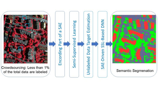
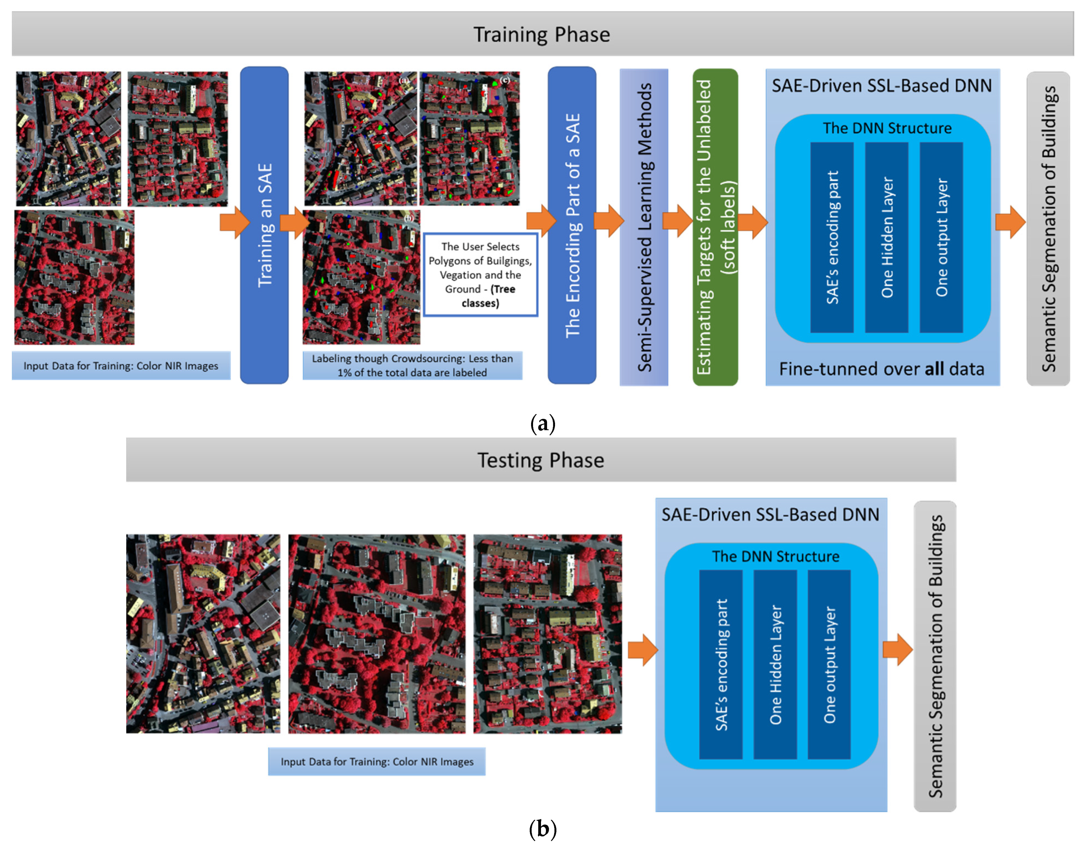
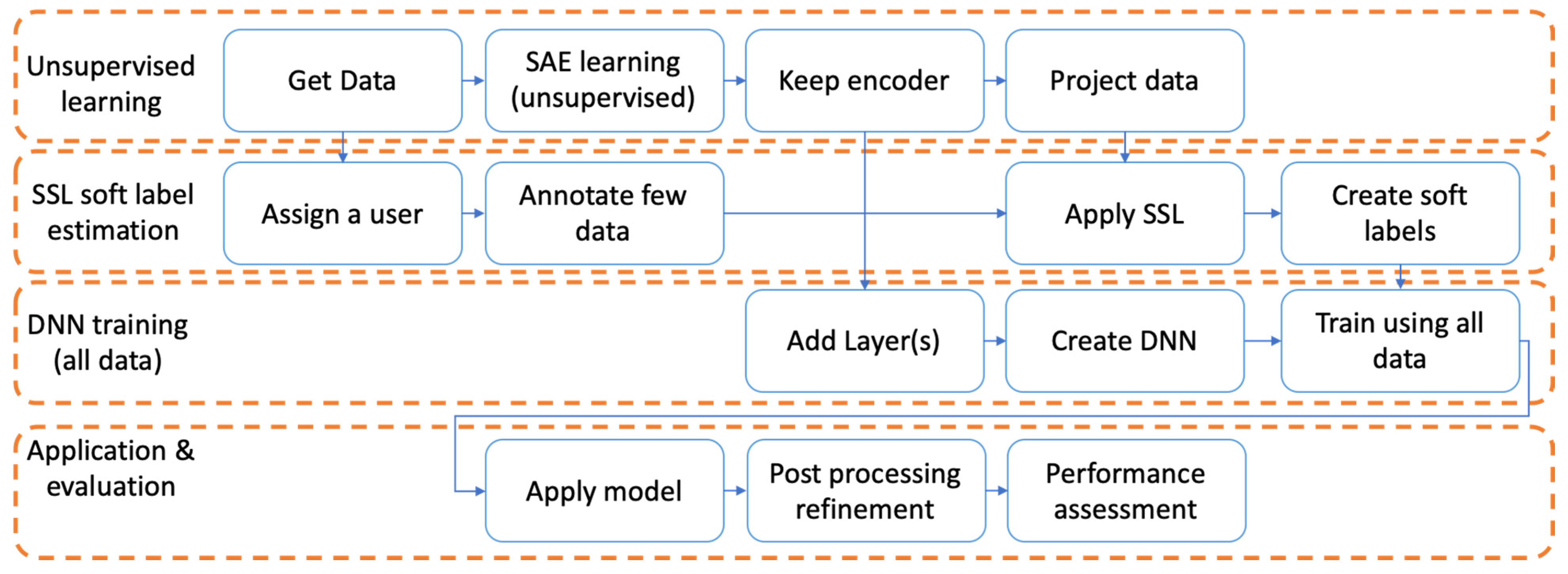
3. Proposed Methodology

3.1. Description of the Overall Architecture

Figure 1 presents a block diagram of the proposed deep learning architecture, used to classify near infrared images into three categories: the buildings, the vegetation and the ground. The two phases are distinguished: the training phase and the testing phase. During the training phase (see Figure 1a), the parameters (weights) of the deep classifier are estimated. During the testing phase (see Figure 1b), NIR data which have not been used in the training phase are fed as inputs to the deep model to carry out the final classification. The proposed approach operates over smaller overlapping image blocks (patches).
The training phase: As for the training, as is shown in Figure 1a, initially, we collect a large set of NIR images. In our case, the data correspond to city areas, located in Germany. We should stress that these data have been used as benchmarked data within the remote sensing community. This way, we can easily compare our results to other state-of-the-art approaches.
More specifically, the NIR input data are split into two subgroups: a small set containing all the label data and a much larger set containing unlabeled ones. The labeled data set includes the corresponding outputs, provided by one or more experts, using a crowdsourcing concept, described in the experimental setup section. The unlabeled dataset does not contain any information on the outputs (no effort for annotating). At this point, we utilize the SSL techniques to estimate soft target values, i.e., labels for the outputs. Before doing so, the input data are no-linearly mapped in a much smaller dimension, using the encoder part of a SAE.
In our case, four SSL schemes are used, which are described in the following section, to generate the soft estimated target outputs (labels) of the unlabeled data; anchor graph, SAFER, SMIR, and a weighted average approach, of the above SSL schemes. The adopted approach results in the creation of a DNN classifier. This module is training using conventional learning strategies such as a backpropagation. The output indicates at which of the three available regions (buildings, vegetation, the ground) each NIR image pixel is assigned to.
The testing phase: Figure 1b shows a block diagram of the testing phase. Different inputs are received by the deep module than the labeled and unlabeled data to classify them into the three class categories. In this case, the encoder part of the SAE is part of the deep structure to reduce the redundant information of the inputs. The SSL schemes are not applicable in this case.
Figure 2 describes the main steps of the proposed solution for enhancing buildings’ classification in NIR images. The methodology adopted consists of four main steps. The first is an unsupervised learning of the SAE to generate proper weights of the model enabling it to carry out the dimensionality reduction. This includes the collection of the data, the construction (training) of the SAE, the retaining of only its encoder part and the projection of the data to reduce their dimensionality. Then, the second step is collection and annotation of a small portion of data through the crowdsource scheme and then the application of an SSL method onto the unlabeled data to approximate (softly) their desired targets. This is done since the SSL schemes are applied on the reduced data inputs x i ( r ) . The third set is the fine tuning (training) of the entire DNN stricture by exploiting all data (labeled and unlabeled ones). Finally, the last fourth step is the application of the model to the test data (unseen).

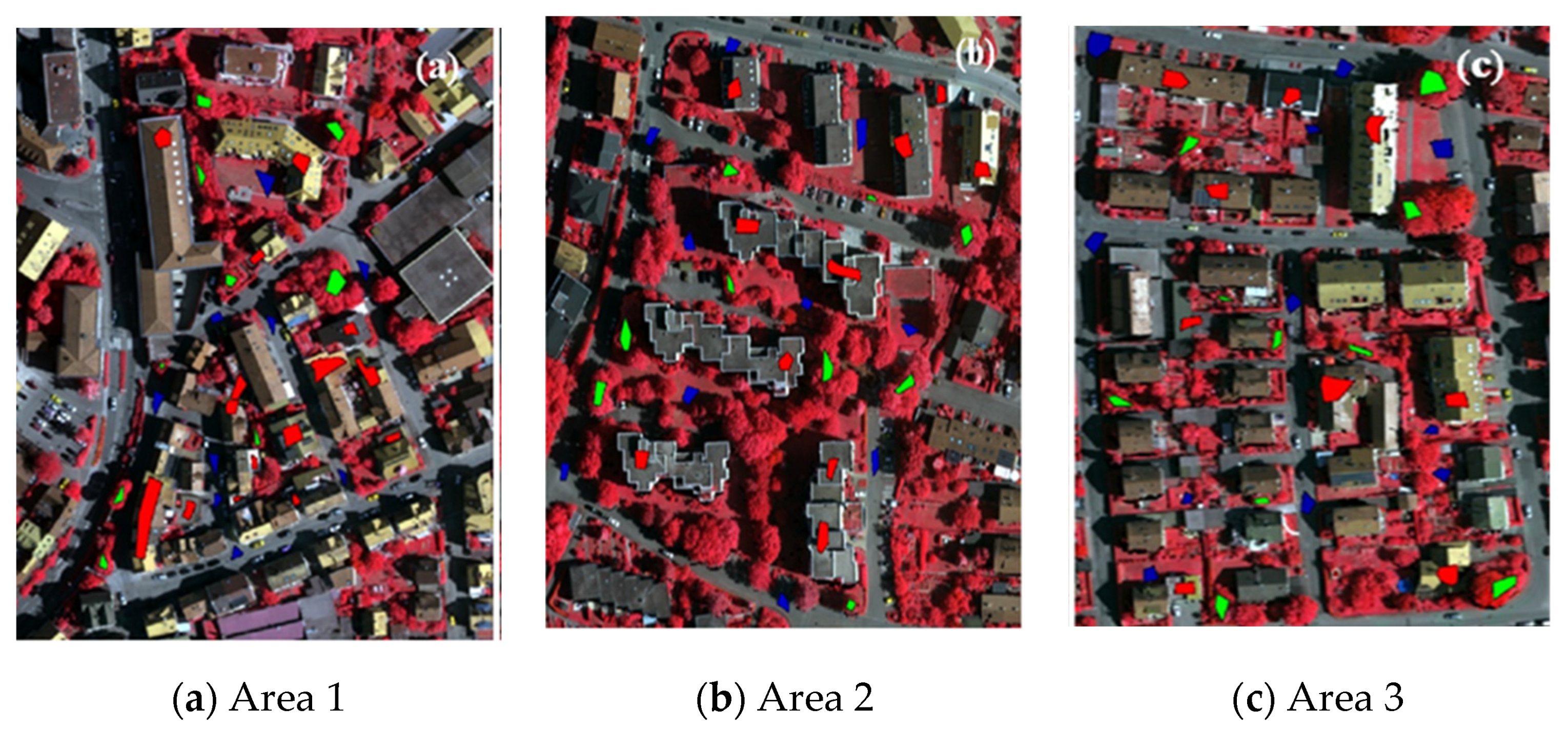
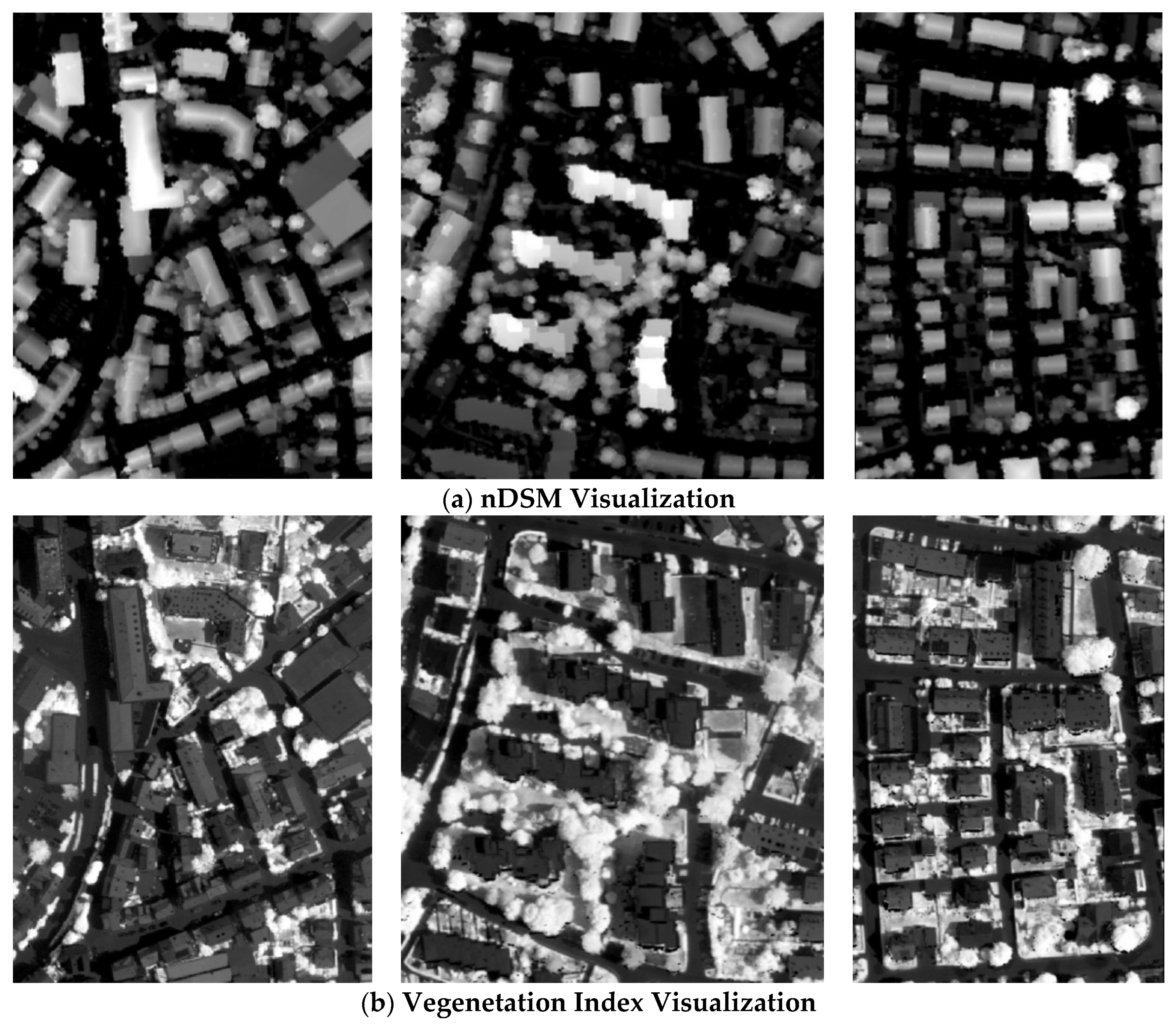
3.2. Description of Our Dataset and of the Extracted Features

Study areas, namely Area 1, Area 2, and Area 3, situated in Vaihingen city in Germany, were used for training and evaluation purposes (Figure 3). The Area 1 mainly consists of historic buildings with notably complex structure; it has sporadically some, often high, vegetation. Area 2 has, mainly, high residential buildings with horizontal multiple planes, surrounded by long arrays or groups of dense high trees. Area 3 is a purely residential area with small, detached houses that consist of sloped surfaces, but there also exists relatively low vegetation. Figure 3 depicts characteristic content of these three areas. In the same figure, we have overlaid small polygons used by the users to select ground truth data of buildings, vegetation and the ground used for the small set of l labeled data.
One interesting case for this dataset is that annotation of the data into two categories, buildings, and non-buildings, is provided. This way, we can benchmark our model outcomes with other state-of-the-art approaches using a reference annotation scheme. In our case, as described in Section 6, two evaluation methods are considered. One using the polygons obtained by our expert users into the three categories (buildings, vegetation, and the ground) and one using the provided benchmarked annotation of the dataset into two categories; buildings and non-buildings (two class classification problem).
Table 1 shows the flying parameters and supplementary information about the used datasets of the Vaihingen study areas as well as the software instruments we use. For the case of the Vaihingen the DSM is extracted from high resolution digital color-infrared (CIR) aerial images applying Dense Image Matching (DIM) methods. These images contain near infrared band (NIR) which is a very good source for the detection of vegetation, exploiting vegetation indexes such Normalized Difference Vegetation Index (NDVI). The CIR aerial images consist of NIR band, Red band, and Green band, and are mainly introduced in [43] in order to contribute to vegetation features. Based on this DIM and DSM, an orthoimage is generated. Table 1 also presents the accuracy and the specification of the generated DSM and DSMs and orthoimages expressed in terms of aerial triangulation accuracy.
A Multi-Dimensional Feature Vector (MDFV) is created to feed the classifier as we have done in one of our earlier works in [20]. The MDFV includes image information from the color components of the NIR images (that is NIR, Red, and Green), the vegetation index, and the height. The vegetation index for every pixel is estimated as
NDVI = NIR R NIR + R
where R and NIR refer to the red and near infrared image band. It should be mentioned that NDVI can be computed only for datasets where the NIR channel is available.
The height is estimated through 3D information of the data. This is accomplished in our case by the application of a Dense Image Matching (DIM) approach to extract the Digital Surface Model (DSM) of the terrain. The cloth simulation and the closest point method [44] are applied to estimate a normalized height from the DSM model using a DIM technique, called normalized DSM (nDSM) [10]. The selected parameters of the cloth simulation algorithm for all the test sites are (i) steep slope and slope processing for the scene, (ii) cloth resolution = 1.5, (iii) max iterations = 500, and (iv) classification threshold = 0.5. This parameter selection provides information similar to a LiDAR system avoiding, however, related acquisition and processing costs of these sensors. Figure 4 shows a visual representation of the two additional feature values used in one MDFV; the normalized nDSM values to measure the height (first row) (see Figure 4a) and the vegetation index (second row) (see Figure 4b).
To avoid labeling the entirety of the images, which is a time-consuming process, only a small ground truth dataset, as a crowdsourcing approach, is employed. By these means, we accelerate the time for constructing the ground truth dataset. In particular, we ask the expert users to draw few polygons over the images. The only limitation is the number of classes. Users had to create (sketch) at least one polygon, which will serve annotation purposes, for each of the following three categories: Buildings (1), Vegetation (2), and Ground (3). This set consists of representative sample polygons for data of each class. Concerning the vegetation class, trees with medium and high height are considered as “good” indicative samples. The ground class contains the bare-earth, roads, and low vegetation (grass, low shrubs, etc.). The class of buildings contains all the man-made structures. To improve classification shadowed areas of each class are also included. In addition, the training sample polygons are spatially created to improve representativity of each class and take into account the spatial coherency of the content. Some examples of these polygons are shown in Figure 3.

3.3. Creation of the Small Portion of Labeled Data (Ground Truth)

Then, we split the annotated data within the polygons into three subsets to train and validate the classifiers. The created subsets, namely labeled, unlabeled, and unseen data, were formed using (approximately) 16, 64, and 20% of the amount within polygons. The labeled and the unlabeled data sets are used to train the network, while the unseen data to test the classifier performance to data different than the ones used in the training. For the labeled data, the desired targets are known. For the unlabeled data the unknown targets (desired outputs) are estimated by transferring knowledge from the labeled samples to the unlabeled ones. The target outputs of the unseen data are estimated from the classifier after training. This constitutes the major advantage of our method, since less than 0.08% among all data are considered as labeled, yet they suffice to create a robust classifier as we will see below, for each of the classes.
Concerning the vegetation class, trees with medium and high height are considered as “good” indicative samples. The ground class contains the bare-earth, roads, and low vegetation (grass, low shrubs, etc.). The class buildings contain all the man-made building structures. To improve the classification process, shadowed areas of each class are also included. In addition, the training sample polygons are spatially created to improve representativity of each class and consider the spatial coherency of the content.
Table 2 demonstrates how the user annotations, using polygons, are distributed for each of the three examined city areas, in each of the three categories. At this point, we should note two things. The annotated data used only are 0.43% for the Area 1, 0.39% for the Area 2 and 0.52% for the Area 3. This includes all data (labeled, unlabeled, and test). Instead the labeled data used is only less than 0.08% of the total data. This number is extremely low number compared to other works, on the same dataset. At first, labeled data, that we use, are 10 times less compared to the work of Maltezos et al. [5], and the much less to the other supervised approaches. Secondly, we have unbalanced datasets for all the areas. Area 1 annotations resulted in a ratio greater than 3 building pixels to 1 of any other categories. Areas 2 and 3 have unbalanced annotated instances, but not as severe as in Area 1.

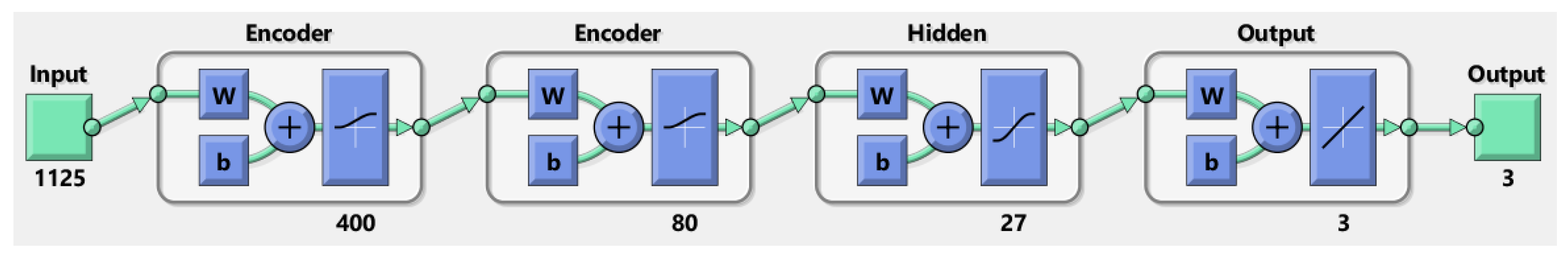
3.4. Setting Up the SAE-Driven DNN Model

Figure 5 illustrates the proposed SAE-driven DNN model. The first two layers correspond to the SAE encoder the weights of which are set through an unsupervised learning process where inputs and outputs are the same [34]. The other two layers of the model are one hidden layer and one output layer responsible to conduct the final classification. Parameters for the hidden and output layers were randomly initialized. Then, a fine-tuning training step, using backpropagation algorithm, is applied to the entire network.
The initial image is separated into overlapping blocks of size 15 × 15 × 5 = 1125 . The DNN classifier utilizes these 1125 values and decides the corresponding class for the pixel at the center of the patch. The first two hidden layers are encoders, trained in an unsupervised way. They serve as non-linear mappers reducing the dimensionality of the feature space from 1125 to 400, and then to 80. Then a hidden layer of 27 neurons perform a final mapping, allowing for the classification in one of the three pre-defined classes.

3.5. Evaluation Metrics

In order to objectively evaluate our results, four different metrics are considered: accuracy, precision, recall, and the critical success index (CSI). We should note that F1-score is directly calculated from precision and recall values. Accuracy (ACC) is defined as:
ACC = TP + TN TP + TN + FP + FN
where the nominator contains the true positives (TP) and true negatives (TN) samples, while denominator contains the TP and TN and false positives (FP) and false negatives (FN). Precision, recall and F1-score are given as
Pr = TP TP + FP   Re = TP TP + FN   F 1 = 2 Pr * Re Pr + Re
Finally, the Critical Success Index (CSI) is defined as
CSI = TP TP + FP + FN  

4. Semi-Supervised Learning Schemes for Softly Labeling the Unlabeled Data

4.1. Problem Formulation

Let us denote X d the set of input data (or features originated from them) and x i as the i-th (feature) input datum, while we assume that n data are available, that is, i = 1, …, n. In this notation variable d denotes the input dimension. As is described in Section 5.1, in our case the input signals are 15 × 15 overlapped patches of NIR images, while for each patch we retain the three-color components (NIR, R and G), the vegetation index (see Equation (1)) and the (normalized) height through Digital Surface Modeling (DSM) measurements, called nDSM. This means that input dimension d = 15 × 15 × 15 = 1125. As we have stated in Section 3.1, only a small portion of the n available data are labeled, say l n . Without loss of generality, we can assume that the first l out of n data are the labeled ones and the remaining n-l the unlabeled ones. Then, for the labeled inputs x i , i = 1, …, l, we know the respective targets (desired outputs) t i . Vectors t i are part of the set T c , where c is the number of classes, equaling three in our case, c = 3, i.e., buildings, vegetation, and the ground. This means that, if we denote as X l = { x 1 , , x l } the set of the labeled input data then we know the target outputs of all these data T = { t 1 , , t l } through an annotation process which, in our case is reliant on a crowdsourcing interface. In the sequel, the pairs ( x i ,   t i ) of input-output relationships can be used through a training procedure to estimate the deep network parameters (weights).
The main drawback of the above-described process is that collecting the annotated (labeled) data is a tough task requiring a lot of manual effort and time. On the contrary, the overwhelming majority of data can be foundin the unlabeled set X u = { x l + 1 , , x n } , for which the desired targets t i , i = l + 1, …, n, are unknown. What we want to do is to approximate these unknown targets and generate reliable estimates t ^ i to be able to include them in the training process and thus to estimate the deep network parameters not only from the small portion of l labeled data but from the large pool of both labeled and unlabeled ones. This way, we have the ambition to improve the classification performance since more information is considered.
In particular, if we denote as ( · ) the loss evaluation function of our deep network and as y w , i the network output when the x i datum is fed as input and the network parameters (weights) are w, then the optimal weighs w ^ are estimated in our semi-supervised learning approach as
w ^ = arg min w   ( Y w ( n ) T ( n ) ) = ( [ y w , 1 y w , l y w , l + 1 y w , n ] [ t 1 t l t ^ l + 1 t ^ n ] )
In this equation, matrices Y w ( n ) = [ y w , 1 y w , n   ] and T ( n ) = [ t w , 1   t w , l   t ^ w , l + 1 t ^ w , n   ] include the network outputs for a specific set of parameters w and respective targets and approximate targets through an SSL scheme. Superscript (n) is added to demonstrate that in this case all the n data (labeled and unlabeled) are taken into account during the training and not only the small portion of l labeled data. This constitutes one of the main novelties of this article.
The second major innovation is the utilization of an SAE compression scheme at a first part of our proposed DNN structure. The goal of this encoding part is, through an unsupervised learning, to map the input set X d to a reduced one X ( r ) o , o d . In our case, only 80 out of 1125 input elements are retained, achieving a dimensionality reduction of 92.89%. The main advantage of such a compression scheme is that we keep only the most salient information of the input data, reducing both computational and memory requirements for training of the DNN, while simultaneously avoiding the learning of “confused” and “contradictory” information due to the high redundancy of the input signals. This means that inputs of the DNN are the signals x i ( r ) of significantly reduced dimension than the original x i .

4.2. The Anchor Graph Method

Anchor graph [40] is a graph-based approach based on a small portion of p < l labeled data, called anchors. These anchors are actual act as representative of the l labeled samples. The anchor samples can form a matrix A = [ a 1 , , a c ] p × c where we recall that c is the number of classes. Thus, A = [ a 1 , , a c ] contains the labels for the representative p samples, in which each column vector accounts for a class. Then, the SSL works so as to minimize the following equation [45]:
min A = [ a 1 , ,   a c ] Q ( A ) = 1 2 | | Z A Ι | | F 2 + γ 2 trace ( A T L ^ A )
where, Z n × p is a sample-adaptive weight matrix that describes how the total n samples are “projected” onto the p anchor samples, L ^ = Z T L Z is a memory-wise and computationally tractable alternative of the Laplacian matrix L . Matrix L n × n , and thus L ^ p × p . The matrix Ι = [ i 1 , , i c ] n × c is a class indicator matrix on ambiguously labeled samples with I i j = 1 if the label l i of the sample i yields the class j and I i j = 0 otherwise.
The Laplacian matrix L , is calculated as L = D W , where D n × n is a diagonal degree matrix and W is given as W = Z Λ 1 Z T . Matrix Λ p × p is defined as: Λ = i = 1 n Z i k , for all k = 1, 2, …, p. The solution of the Equation (4) has the form of [45]:
A * = ( Z T Z + γ L ^ ) Z T Y
where A * is the optimal estimation of matric A. Scalar γ of Equations (6) and (7) defines the weighted degree of the second term of both equations. Then, each sample label is, then, given by:
l ^ i = arg max j { 1 , ,   c } Z i a j λ j
where Z i 1 × p denotes the i -th row of Z , and factor λ j   =   1 T   Z   α j balances skewed class distributions.

4.3. SAFER: Safe Semi-Supervised Regression

Assume a set of b semi-supervised classifiers of soft outputs (hence, we can call these models as semi-supervised regressors-SSRs) applied over the unlabeled set X u . The outcome would be b predictions, i.e., { f 1 , , f b } , where f i = { f i ( x 1 ) , , f i ( x l ) } , i = 1 , , b . Let as, also, denote as f 0 the model output over the same unlabeled set X u of a known traditional supervised approach using as targets the estimated unlabeled outputs. For each regressor, we set a significance weight a i 0 . Then, we would like to find the optimal regressor, f, so that [41]:
max f i = 0 b a i ( | |   f 0   f i | | 2 | | f   f i | | 2 )
In Equation (9), both the optimal soft classifier output (the regression f) and the weights a = [ a 1 a b ] are unknown. To solve this problem, we constrain the weights so that a 0 and 1 T a 1 , that is, the sum of all weights should be one [46]. Then, we have a linear programming problem as follows:
max f min a i = 0 b a i ( | |   f 0   f i | | 2 | | f   f i | | 2 )
where the set = { a |   1 T a = 1 , and   a 0 } . The equation above is concave to f and convex to a and thus it is recognized as saddle-point convex-concave optimization [34]. As described in recent work [16], Equation (5) can be formulated as a geometric projection problem, handling that way the computational load. Specifically, by setting the derivative of Equation (10) to zero, we get a close form solution with respect to f and a as:
min a | | i = 1 b a i f i f 0 | |   and   f = i = 1 b a i f i
Using Equation (11), we can initially estimate the optimal weight coefficients through the first term of the above-mentioned equation while then the optimal regression is estimated through the second term.

4.4. SMIR: Squared-Loss Mutual Information Regularization

The Squared-loss Mutual Information Regularization (SMIR) is a probabilistic framework trained in an unsupervised way so that a given information measure between data and cluster assignments is maximized (how well the clusters will represent the data). Maximization is achieved through a convex optimization strategy (under some mild assumptions regarding cluster overlapping) and thus it results in a global optimal solution [42].
For a given input x X we would like to estimate to which class this input is assigned to by maximizing the probability t ^ = arg max t p ( t | x ) . In this notation, we adopt a scalar network output t instead of a vector one. This is not a real restriction since any vectorized output of finite c classes can be mapped onto one-dimensional space. The described SMIR approach approximates the class-posterior probability p ( t | x ) as follows. Assuming a uniform class-prior probability p ( t ) = 1 / c (equal importance of all output classes), the Square-loss Mutual Information (SMI) (without the use of the regularization terms) has the following form [47]:
S M I = c 2 X t ϵ T ( p ( t | x ) ) 2 p ( x ) d x 1 2
To unknown probability p ( t | x ) of Equation (12) can be approximated as a kernel model
q ( t | x ; A ) = i n a t , i k ( x , x i )
where q ( · ) is the approximate of the probability p ( t | x ) and A = [ a 1 a c ]   n × c , where a vector element of A is given as a r = [ a r , 1 , , a r , n ] T   are model parameters and k ( · ) is the kernel X × X which takes two inputs and returns a scalar. If we approximate the probability p ( x ) of Equation (12) as the empirical average then the SMI approach is given as
S M I ^ = c 2 n t T a t T · K 2 · a t 1 2
where K n × n   is the kernel matric overall all n samples.
In principle, any kernel model linear with respect to a t can be used to approximate the probability p ( t | x ) . However, this may lead to a non-convex optimization and thus the optimal solution can be trapped to local minima. To avoid this, in [42] a regularization term is adopted. This is done by introducing a new kernel Φ n which maps the inputs from the input space X to the n-dimensional space n , that is,
Φ n : X n , x [ k ( x , x 1 ) , , k ( x , x n ) ] T
If we denote as d i = j = 1 n k ( x i , x j ) the degree of x i and as D = d i a g ( d 1 , d 2 , , d n ) the degree diagonal matrix, then we can approximate the class posterior probability p ( t | x ) by
q ( t | x ; A ) = K 1 2 Φ n ( x ) , D 1 2 a t
where 〈·〉 is the inner product. This equation is valid assuming that K is a full rank matrix and K 1 2 is well defined. Plugging Equation (16) into (12), we can have an alternative the SMI criterion alternated with a regularization term called Squared-loss Mutual Information Regularization (SMIR) which is given as
S M I R ^ = c 2 n t r ( A T D 1 2 K D 1 2 A ) 1 2
where A n × c is the matrix representation of model’s parameters as in Equation (13).
Equation (17) is used to regularize a loss function Δ ( p , q ) of the actual class posterior probability p ( ) and its approximate version q ( ) . Function Δ ( , ) expresses how much the actual probability divers to the approximate one. Then, we can have as objective (i) to minimize Δ ( p , q ) , (ii) to maximize S M I R ^ and (iii) to regularize model parameters A . Hence, the SMIR optimization problem is formulated as:
min a 1 , , a c     n Δ ( p , q ) γ S M I R ^ + λ y 1 2 | | α t | | 2 2
where γ , λ > 0 are regularization parameters. If the kernel function k ( · ) is nonnegative and λ > γ c n , Equation (18) is convex and always converges to a global optimum. Thus, we can threshold λ to be greater than a specific value to guarantee the convexity property.
Under these regularization schemes, the optimal estimation of the class posterior p ( t | x ) is given as 42:
p ^ ( t | x ) = m a x ( 0 , Φ n ( x ) , β t ) j = 1 c m a x ( 0 , Φ n ( x ) , β j )
with
β t = n π t K 1 2 D 1 2 a t * 1 n T K 1 2 D 1 2 a t *
In Equation (20),   β t is a normalized version of the optimal model parameters a t * and π t an estimate of the probability p ( t ) .

5. Experimental Results

5.1. Data Post Processing

To purify the output of the classifier from the noisy data, initially only the building category is selected from the available classes. The building mask is refined by post processing. The goal of the post processing is to remove noisy regions such as isolated pixels or tiny blobs of pixels and retains local coherency of the data. Towards this, initially a majority voting technique with a radius of 21 pixels is implemented. Additionally, an erosion filter of a 7 × 7 window is applied.
The majority voting filter categorizes the potential building block with respect to the outputs of the neighboring output data. This filter addresses the spatial coherency that a building has. Since the orthoimages generated based on DSMs, the building boundaries are blurred due to mismatches during the application DIM algorithm. This affects the building results dilating their boundaries. Thus, the erosion filter was applied to “absorb” possible excessive interpolations on the boundaries of the buildings by reducing their dilated size.

5.2. Performance Evaluation

A total of two alternative approaches are considered for the evaluation of the model performance: (i) over the polygons-bounded areas in which the three class categories are discriminated (buildings, vegetation and ground) and (ii) over the original annotations provided by the dataset. This includes only two categories; the buildings and the non-buildings class as stated in Section 3.2. The first evaluation case is a typical multiclass classification problem while the second entails to a binary classification.

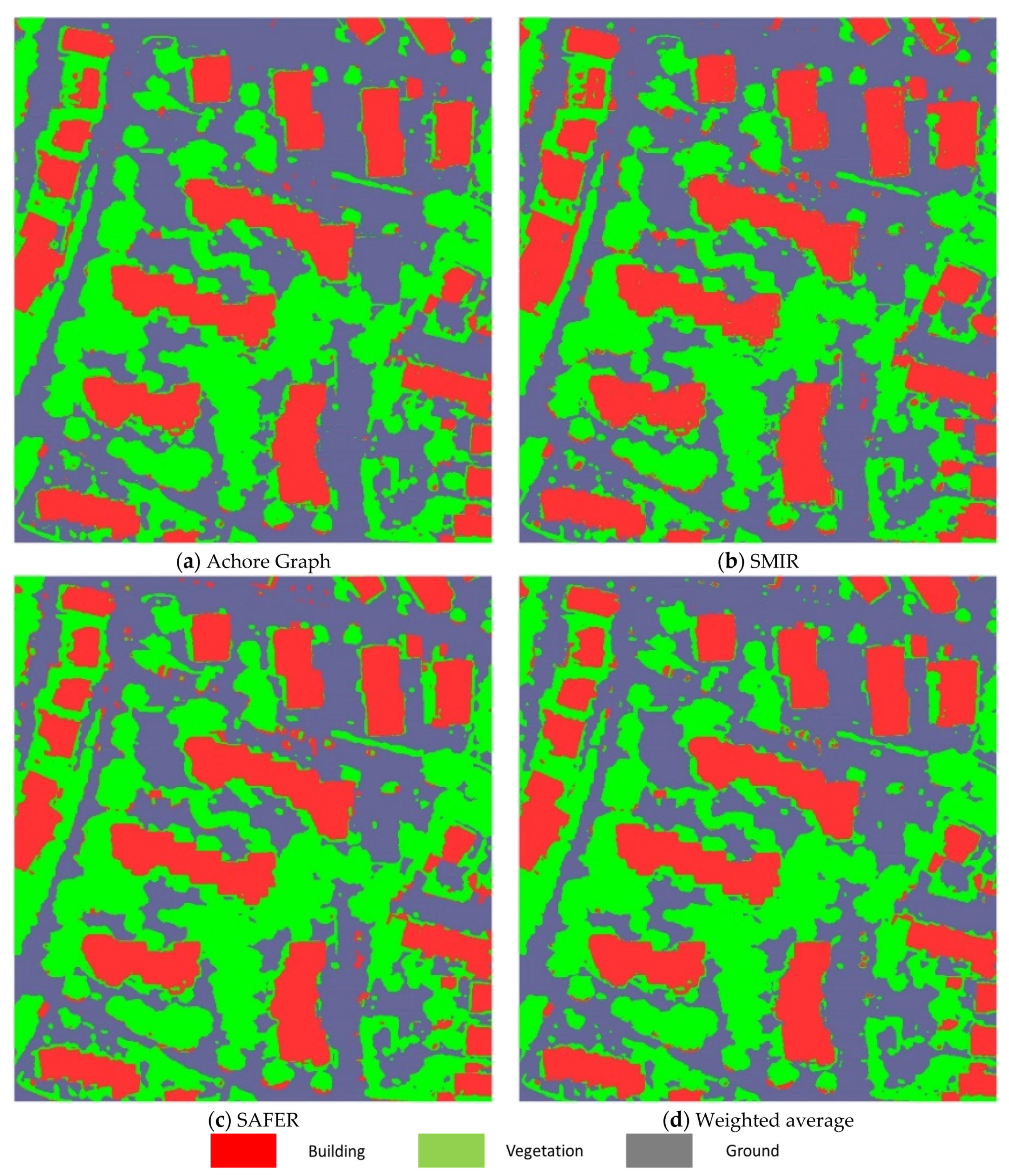
5.2.1. The Multi-Class Evaluation Approach

In this scenario, we evaluate the performance of our model over the three available classes, i.e., Buildings (1), Vegetation (2), and the Ground (3), given the annotated samples from the crowdsourced data. The SAE-driven and SSL-based DNN model has been trained using the small portion of labeled data and the unlabeled ones. Regarding the unlabeled data, one of the proposed SSL is applied to estimate the targets and through them to accomplish the model training.
Table 3 demonstrates the proposed model performance over the unlabeled and unseen (test) data. This means that, after having training the model using both labeled and unlabeled data, we feed as inputs to the classifier only the unlabeled and the unseen data to evaluate its classification performance. The use of the unseen (test) set is made to assess the model performance to data totally outside the training phase, i.e., to data that the model has not seen during the learning process. The use of unlabeled data is to assess how well the model behaves with the amount of data, the targets of which have been estimated by the SSL methods; i.e., how well the selected SSL techniques work. The results have been obtained using the Accuracy, Precision, and Recall objective criteria (see Section 3.5) for all the three examined areas, averaging out over all of them and over all categories.
We can see that high-performance results are obtained. The results are slightly better when the simple fusion SSL method, called WeiAve is employed, but it seems that all SSL techniques work very well in correctly estimating the unlabeled and test data.
Ablation Study: We now proceed to an ablation study to indicate how the different components of our system affect the final performance. First, we examine how well the proposed SSL algorithms work. Table 4 presents how well the four proposed SSL algorithms can estimate the actual targets (labels) of the unlabeled samples. That is, we have compared the soft labeled generated by the four SSL schemes with the actual ones assigned by the expert users. Evaluation is carried out for the three examined Areas and using two objective criteria; the root means squared error and the F1-score. As is observed, all the proposed SSL schemes correctly estimates the labels of the data.
Another ablation analysis is to examine how well our model behaves without the use of the SSL and SAE schemes, that is, without the use of the two main components of our approach. Towards this, initially we train the DNN model using both the labeled and the unlabeled data but for the latter we treat them as labeled ones considering in the training the actual targets of the unlabeled data. Then, we evaluate the performance of the trained DNN on the unseen (test) data. Table 5 shows the results obtained using three objective criteria; Accuracy, Precision, and Recall by averaging out on the three examined Areas. In this table, we show present the results of the WeiAve SSL approach of Table 3 for direct comparisons. As we can see, the results are very close which is justified from the fact that the SSL methods can correctly estimates the labels of the data (see Table 4). However, the disadvantage of including treating unlabeled data as labeled is the additional manual effort needed to generate these new labels and the extra human and financial resources this imposes on. Thus, our approach yields the same classification performance but with a much smaller portion of labeled data.
In the same Table 5, we also present classification results when we remove the SAE encoding part from the network. First, such as process dramatically increases the computational cost needed for training and the memory requirements due to the high dimension of the input signals. In addition, the classification results seem to be worsened. This is due to the noise embedded from the high information redundancy the input signals carry out. Thus, the SAE scheme not only reduces the computational and memory costs for the training but it also eliminates information noise in the inputs which may confuse classification.
In Table 6, we depict the computational cost imposed for the four SSL schemes, the time needed for the whole system to classify all pixels of the image, and the time for the SAE component to reduce information redundancy. We observe that SMIR is the fastest SSL technique requiring only few seconds to be completed. Instead, SAFER is much slower. The SAE encoding takes a lot of time but this is activated only in the training phase of the classifier. The time needed to classify the full image pixels is also depicted in Table 6. Recall that annotation requires the creation of overlapping patches of size 15 x 15. In our case, we use simple loop parsing for such creation. Numerical tensor manipulation could result in significantly reduced time.

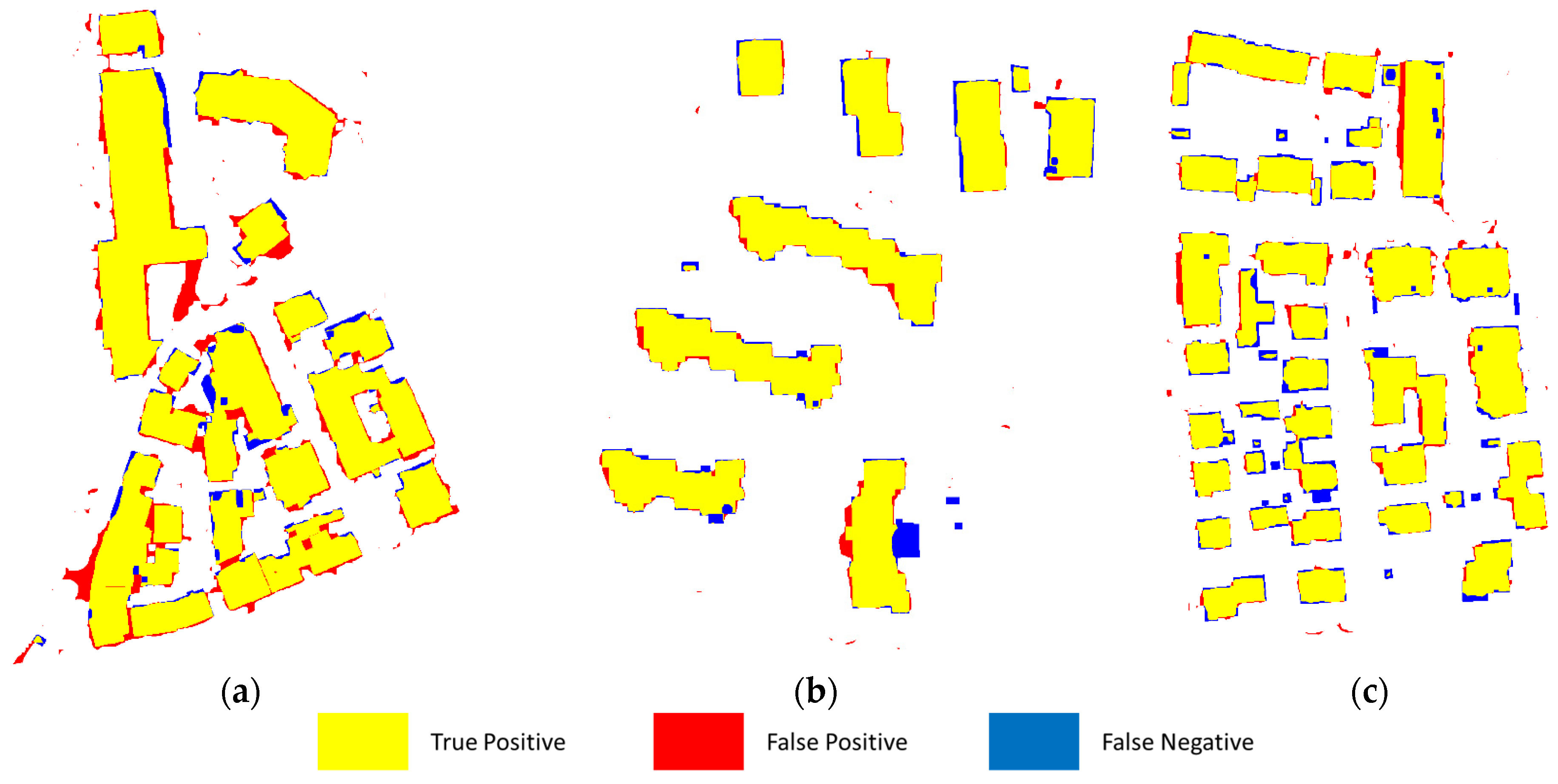
5.2.2. Class Evaluation Approach

In this case, the evaluation is carried out on the provided annotation of the dataset which assesses the data into two categories: the buildings and the non-buildings. This way, we can provide a comparative analysis of our results to other approaches. Table 7 shows the results obtained in this case as the average over the two class categories using the objective criteria of Recall, Precision, F1-score, and Critical Success Index (CSI). The results are displayed for the three examined areas and the four different SSL methods. The highest F1 scores are achieved when the WeiAve approach is adopted for areas 1 and 2. Area 3 best score is achieved using SAFER technique. All cases result in high scores. In the same table, the ranking order of each method is also displayed.
Figure 6 demonstrates the DNN classifier’s performance over small objects (e.g., single trees). Pixel annotation similarity exceeds 85% for all images. Generally, when the object spans less than 10 × 10 pixels, detection capabilities decline. This could be partially explained since most of the block pixels, i.e., ( 15 × 15 ) ( 10 × 10 ) = 125 pixels, describe something different. The best DNN model, in this case, is trained using the WeiAve SSL scheme.
Figure 7 evaluates against the ground truth data the building detection capabilities of our model for the three examined areas. In particular, as for Figure 7a,b of Areas 1 and 2, the WeiAve SSL technique has been applied to estimate the soft labels of the unlabeled data used during the training phase. For the Area 3, the SAFER SSL is exploited. This differentiation is adopted since WeiAve best performs for Area 1 and Area 2 while SAFER is the best for Area 3. Yellow color corresponds to pixels showing a building and model classified them as building (True Positive). Red color indicates pixels that model classified as buildings, but the actual label was either vegetation or ground (False Positive). Finally, blue color indicates areas that are buildings, but model failed to recognize them (False Negative). As is observed, segmentation for building blocks is extremely accurate considering the limited training sample. Misclassification involved inner yards, kiosk size buildings (e.g., bus stations), and the edges of the buildings.

5.2.3. Comparison with Other State-of-the-Art Approaches

In this section, we compare the performance of our approach with other state-of-the-art techniques exploited the same dataset as ours. This is the main value of selecting a benchmarked dataset for conducting our experiments, i.e., direct comparison of our results with other methods. Table 8 presents the comparison results. More specifically, in this table, we show our results using the proposed SAE-driven and SSL-based DNN in case that different SSL techniques are applied for labeling the unlabeled data. We also compare our results against other state-of-the-art methods using (a) the same type of data (orthoimage plus height estimation using DIM and DSM modeling), (b) combining orthoimages with expensive LiDAR information, (c) applying only expensive LiDAR information on the analysis. All the results have been obtained using the CSI score.
Our method outperforms all the state-of-the-art methods using the same data types (low-cost orthoimages plus an estimation of the height through DIM and DSM). If the expensive and more precise LiDAR information is utilized the results are slightly better and in some cases (like the work of [48]) even worse than our case. This reveals that our method, although it exploits only a cheap and not so precise height extracted information, gives results of similar performance. We should also stress that in our approach only less than 0.08% of the total data is utilized for a labeled training significantly reducing the effort required to annotate the data. As a result, it is clear that our methodology gives similar performance to state-of-the-art techniques though the fact that we use a very limited dataset, and relative cheap orthoimage information instead of high expensive LiDAR one.

6. Discussion

The main problem in classifying satellite remote sensing data into semantic categories is the creation of an annotated (labeled) dataset needed for the training process. This dataset creation requires high manual effort which is a time consuming and costly process. In addition, data annotation also means waste of human and financial resources which make the whole process unaffordable. The main innovation of this paper is the utilization of a very small labeled dataset for semantic segmentation of remote sensing NIR data. The utilization of a very small labeled dataset reduces the cost for the annotation and better utilizes the experts in conducting remote sensing works rather than annotating data to create labels. However, a reduction in the number of training data will result in a deterioration of the classification accuracy as well. To compensate this, we adopt the concept of semi-supervised learning (SSL). The goal of an SSL scheme is to enrich the model training phase with additional unlabeled data, the targets of which are estimated by transferring knowledge from the small labeled dataset to the unlabeled one. Furthermore, a non-linear encoding scheme is adopted through the use of Stacked Auto-encoders (SAE) to remove information redundancy from the input signals.
The experiments show that the proposed SSL schemes can very well estimate the labels of the unlabeled data within an accuracy of almost 99.9%. This implies that we can reduce the labeled dataset even ten times than other state-of-the-art works while keeping classification performance almost the same. In our case only up to 0.08% of the total data are used as labeled data. In addition, the experiments show that the proposed scheme yields classification results very close to the ones obtained using high cost sensors such as LiDAR.
The advantages of our proposed SAE-driven and SSL-boosted DNN model are: (a) limited effort and time to construct the training set, since few labeled data (i.e., less than 0.08% when the closest supervised approach use approximately ten times more data [10]) are required for training, (b) adaptability to user needs, since user can define the number and the type of classes to classify (thus, we can easily apply the same concept to different case scenarios, e.g., classification of different types of objects instead of buildings), and (c) applicability in the sense that the proposed scheme supports the transfer learning concept, since a pretrained network can be easily updated to handle different types of problems.

7. Conclusions

In this paper we employ semi-supervised learning (SSL) methods with Stacked Auto-encoders (SAE) for semantically segmenting NIR remote sensing images. The SSL schemes transfer knowledge from a small set of labeled data to estimate the targets (soft labels) of the unlabeled data. Then, deep neural network training is carried out using only this small portion of labeled samples and the estimated labels of the vast amount of unlabeled data to correctly train the network. As a result, the effort required to annotate the data is minimize while training is keeping at acceptable levels. Overall, four SSL methods are adopted for estimating the targets of the unlabeled samples; the Anchor Graph, SAFE Semi-Supervised Regression (SAFER), the Squared-loss Mutual Information Regularization (SMIR) and an equal importance Weighted Average of them, called (WeiAve).
Another novelty of our paper is the use of a Stack Autoencoder (SAE) scheme to reduce redundancy in the input signals, while keeping almost all the meaningful information. The goal of the SAE encoding is to map the input data into a much smaller dimensional space but under a highly non-linear way to retain most of the knowledge within the input samples. This way, we avoid noisy effects in the signals and potential contradictory information.
The combination of the above-mentioned novelties yields to a new proposed deep learning model which is called SAE-driven SSL-based Deep Neural Network (DNN). The selection of a DNN instead of a Convolutional Neural Network (CNN) model is to overcome the dimensionality of the inputs when they are propagated into multiple convolutions. The model is tested regarding its classification performance on a benchmarked dataset such as the Vaihingen city in Germany to allow us to directly compare our approach with other state-of-the-art methodologies. The results show that our approach outperforms the compared works in case that they exploit orthoimages as data types. This is achieved, although an exceedingly small portion of less than 0.08% of the total data have been used for the labeling set. We have also compared our method with methodologies employing highly sensitive but much more expensive sensors such as LiDAR information. The results indicate that our methodology yield close results to the ones obtained by LiDAR samples despite the fact that our data are much less precise and a very small portion of labeled samples is utilized.

Author Contributions

Conceptualization, E.P. and A.D.; methodology, E.P., A.D. and N.D.; software, E.P. and E.M.; validation, E.P., A.D. and N.D.; formal analysis, E.P., A.D. and N.D.; investigation, E.P. and A.D.; resources, A.D., N.D. and E.M.; data curation, E.P. and E.M; writing—original draft preparation, E.P. and N.D.; writing—review and editing, E.P., A.D., N.D.; visualization, E.P., A.D. and E.M.; supervision, A.D. and N.D.; project administration, A.D.; funding acquisition, A.D. and N.D. All authors have read and agreed to the published version of the manuscript.

Funding

This research was funded by the Innovation and Networks Executive Agency (INEA) under the powers delegated by the European Commission through the Horizon 2020 program “PANOPTIS–Development of a decision support system for increasing the resilience of transportation infrastructure based on combined use of terrestrial and airborne sensors and advanced modelling tools”, Grant Agreement number 769129.

Informed Consent Statement

Not applicable.

Data Availability Statement

The data presented in this study are openly available in ISPRS Test Project on Urban Classification, 3D Building Reconstruction and Semantic Labeling https://www2.isprs.org/commissions/comm2/wg4/benchmark/detection-and-reconstruction/.

Acknowledgments

The Vaihingen dataset was provided by the German Society for Photogrammetry, Remote Sensing, and Geoinformation (DGPF).

Conflicts of Interest

The authors declare no conflict of interest.

References

  1. Makantasis, K.; Karantzalos, K.; Doulamis, A.; Loupos, K. Deep learning-based man-made object detection from hyperspectral data. In Proceedings of the International Symposium on Visual Computing (ISCV 2015), Las Vegas, NV, USA, 14–16 December 2015; pp. 717–727. [Google Scholar]
  2. Karantzalos, K. Recent advances on 2D and 3D change detection in urban environments from remote sensing data. In Computational Approaches for Urban Environments; Springer: Berlin/Heidelberg, Germany, 2015; pp. 237–272. [Google Scholar]
  3. Doulamisa, A.; Doulamisa, N.; Ioannidisa, C.; Chrysoulib, C.; Grammalidisb, N.; Dimitropoulosb, K.; Potsioua, C.; Stathopouloua, E.K.; Ioannides, M. 5D modelling: An efficient approach for creating spatiotemporal predictive 3d maps of large-scale cultural resources. ISPRS Ann. Photogramm. Remote Sens. Spat. Inf. Sci. 2015. [Google Scholar] [CrossRef] [Green Version]
  4. Zou, S.; Wang, L. Individual Vacant House Detection in Very-High-Resolution Remote Sensing Images. Ann. Am. Assoc. Geogr. 2020, 110, 449–461. [Google Scholar] [CrossRef]
  5. Wei, Y.; Feng, J.; Liang, X.; Cheng, M.M.; Zhao, Y.; Yan, S. Object region mining with adversarial erasing: A simple classification to semantic segmentation approach. In Proceedings of the IEEE Conference on Computer Vision and Pattern Recognition, Honolulu, HI, USA, 21–26 July 2017; pp. 1568–1576. [Google Scholar]
  6. Sorzano, C.O.S.; Vargas, J.; Montano, A.P. A survey of dimensionality reduction techniques. arXiv 2014, arXiv:1403.2877. [Google Scholar]
  7. Qiu, W.; Tang, Q.; Liu, J.; Teng, Z.; Yao, W. Power Quality Disturbances Recognition Using Modified S Transform and Parallel Stack Sparse Auto-encoder. Electr. Power Syst. Res. 2019, 174, 105876. [Google Scholar] [CrossRef]
  8. Voulodimos, A.; Doulamis, N.; Doulamis, A.; Protopapadakis, E. Deep learning for computer vision: A brief review. Comput. Intell. Neurosci. 2018, 2018, 7068349. [Google Scholar] [CrossRef]
  9. Schenkel, F.; Middelmann, W. Domain Adaptation for Semantic Segmentation Using Convolutional Neural Networks. In Proceedings of the IEEE International Geoscience and Remote Sensing Symposium (IGRASS), Yokohama, Japan, 28 July–2 August 2019; pp. 728–731. [Google Scholar] [CrossRef]
  10. Maltezos, E.; Doulamis, A.; Doulamis, N.; Ioannidis, C. Building extraction from LiDAR data applying deep convolutional neural networks. IEEE Geosci. Remote Sens. Lett. 2018, 16, 155–159. [Google Scholar] [CrossRef]
  11. Makantasis, K.; Karantzalos, K.; Doulamis, A.; Doulamis, N. Deep supervised learning for hyperspectral data classification through convolutional neural networks. In Proceedings of the IEEE International Geoscience and Remote Sensing Symposium (IGARSS), Milan Italy, 26–21 July 2015; pp. 4959–4962. [Google Scholar]
  12. Du, S.; Zhang, Y.; Zou, Z.; Xu, S.; He, X.; Chen, S. Automatic building extraction from LiDAR data fusion of point and grid-based features. ISPRS J. Photogramm. Remote Sens. 2017, 130, 294–307. [Google Scholar] [CrossRef]
  13. Hou, B.; Wang, Y.; Liu, Q. A saliency guided semi-supervised building change detection method for high resolution remote sensing images. Sensors 2016, 16, 1377. [Google Scholar] [CrossRef] [Green Version]
  14. Ham, S.; Oh, Y.; Choi, K.; Lee, I. Semantic Segmentation and Unregistered Building Detection from Uav Images Using a Deconvolutional Network. Int. Arch. Photogramm. Remote Sens. Spat. Inf. Sci. 2018, 42. [Google Scholar] [CrossRef] [Green Version]
  15. Liu, X.; Deng, Z.; Yang, Y. Recent progress in semantic image segmentation. Artif. Intell. Rev. 2019, 52, 1089–1106. [Google Scholar] [CrossRef] [Green Version]
  16. Awrangjeb, M.; Fraser, C.S.; Lu, G. Building change detection from LiDAR point cloud data based on connected component analysis. ISPRS Ann. Photogramm. Remote Sens. Spat. Inf. Sci. 2015, 2, 393. [Google Scholar] [CrossRef] [Green Version]
  17. Kashani, A.G.; Olsen, M.J.; Parrish, C.E.; Wilson, N. A review of LiDAR radiometric processing: From ad hoc intensity correction to rigorous radiometric calibration. Sensors 2015, 15, 28099–28128. [Google Scholar] [CrossRef] [PubMed] [Green Version]
  18. Nahhas, F.H.; Shafri, H.Z.; Sameen, M.I.; Pradhan, B.; Mansor, S. Deep learning approach for building detection using lidar–orthophoto fusion. J. Sens. 2018, 2018, 7212307. [Google Scholar] [CrossRef] [Green Version]
  19. Zhou, K.; Gorte, B.; Lindenbergh, R.; Widyaningrum, E. 3D building change detection between current VHR images and past lidar data. Int. Arch. Photogramm. Remote Sens. Spat. Inf. Sci. 2018, 42, 1229–1235. [Google Scholar] [CrossRef] [Green Version]
  20. Maltezos, E.; Protopapadakis, E.; Doulamis, N.; Doulamis, A.; Ioannidis, C. Understanding Historical Cityscapes from Aerial Imagery Through Machine Learning. In Proceedings of the Digital Heritage. Progress in Cultural Heritage: Documentation, Preservation, and Protection, Nicosia, Cyprus, 29 October–3 November 2018. [Google Scholar]
  21. Nguyen, T.H.; Daniel, S.; Gueriot, D.; Sintes, C.; Caillec, J.-M.L. Unsupervised Automatic Building Extraction Using Active Contour Model on Unregistered Optical Imagery and Airborne LiDAR Data. In Proceedings of the ISPRS—International Archives of the Photogrammetry, Remote Sensing and Spatial Information Sciences, Munich, Germany, 18–20 September 2019; Volume XLII-2/W16, pp. 181–188. [Google Scholar] [CrossRef] [Green Version]
  22. Dos Santos, R.C.; Pessoa, G.G.; Carrilho, A.C.; Galo, M. Building detection from lidar data using entropy and the k-means concept. Int. Arch. Photogramm. Remote Sens. Spat. Inf. Sci. 2019. [Google Scholar] [CrossRef] [Green Version]
  23. Huang, R.; Yang, B.; Liang, F.; Dai, W.; Li, J.; Tian, M.; Xu, W. A top-down strategy for buildings extraction from complex urban scenes using airborne LiDAR point clouds. Infrared Phys. Technol. 2018, 92, 203–218. [Google Scholar] [CrossRef]
  24. Cai, Z.; Ma, H.; Zhang, L. A Building Detection Method Based on Semi-Suppressed Fuzzy C-Means and Restricted Region Growing Using Airborne LiDAR. Remote Sens. 2019, 11, 848. [Google Scholar] [CrossRef] [Green Version]
  25. Yang, H.; Wu, P.; Yao, X.; Wu, Y.; Wang, B.; Xu, Y. Building extraction in very high resolution imagery by dense-attention networks. Remote Sens. 2018, 10, 1768. [Google Scholar] [CrossRef] [Green Version]
  26. Ji, S.; Wei, S.; Lu, M. Fully convolutional networks for multisource building extraction from an open aerial and satellite imagery data set. IEEE Trans. Geosci. Remote Sens. 2018, 57, 574–586. [Google Scholar] [CrossRef]
  27. Shrestha, S.; Vanneschi, L. Improved fully convolutional network with conditional random fields for building extraction. Remote Sens. 2018, 10, 1135. [Google Scholar] [CrossRef] [Green Version]
  28. Yang, H.L.; Yuan, J.; Lunga, D.; Laverdiere, M.; Rose, A.; Bhaduri, B. Building extraction at scale using convolutional neural network: Mapping of the united states. IEEE J. Sel. Top. Appl. Earth Obs. Remote Sens. 2018, 11, 2600–2614. [Google Scholar] [CrossRef] [Green Version]
  29. Huang, J.; Zhang, X.; Xin, Q.; Sun, Y.; Zhang, P. Automatic building extraction from high-resolution aerial images and LiDAR data using gated residual refinement network. ISPRS J. Photogramm. Remote Sens. 2019, 151, 91–105. [Google Scholar] [CrossRef]
  30. Chen, K.; Weinmann, M.; Gao, X.; Yan, M.; Hinz, S.; Jutzi, B.; Weinmann, M. Residual shuffling convolutional neural networks for deep semantic image segmentation using multi-modal data. ISPRS Ann. Photogramm. Remote Sens. Spat. Inf. Sci. 2018, 4. [Google Scholar] [CrossRef] [Green Version]
  31. Makantasis, K.; Doulamis, A.D.; Doulamis, N.D.; Nikitakis, A. Tensor-based classification models for hyperspectral data analysis. IEEE Trans. Geosci. Remote Sens. 2018, 56, 6884–6898. [Google Scholar] [CrossRef]
  32. Makantasis, K.; Doulamis, A.; Doulamis, N.; Nikitakis, A.; Voulodimos, A. Tensor-based nonlinear classifier for high-order data analysis. In Proceedings of the 2018 IEEE International Conference on Acoustics, Speech and Signal Processing (ICASSP), Calgary, AB, Canada, 15–18 April 2018; pp. 2221–2225. [Google Scholar]
  33. Li, X.; Zhang, L.; Du, B.; Zhang, L.; Shi, Q. Iterative Reweighting Heterogeneous Transfer Learning Framework for Supervised Remote Sensing Image Classification. IEEE J. Sel. Top. Appl. Earth Obs. Remote Sens. 2017, 10, 2022–2035. [Google Scholar] [CrossRef]
  34. Protopapadakis, E.; Voulodimos, A.; Doulamis, A.; Doulamis, N.; Dres, D.; Bimpas, M. Stacked autoencoders for outlier detection in over-the-horizon radar signals. Comput. Intell. Neurosci. 2017, 2017, 5891417. [Google Scholar] [CrossRef]
  35. Li, W.; Fu, H.; Yu, L.; Gong, P.; Feng, D.; Li, C.; Clinton, N. Stacked Autoencoder-based deep learning for remote-sensing image classification: A case study of African land-cover mapping. Int. J. Remote Sens. 2016, 37, 5632–5646. [Google Scholar] [CrossRef]
  36. Liang, P.; Shi, W.; Zhang, X. Remote sensing image classification based on stacked denoising autoencoder. Remote Sens. 2018, 10, 16. [Google Scholar] [CrossRef] [Green Version]
  37. Song, H.; Kim, M.; Park, D.; Lee, J.-G. Learning from noisy labels with deep neural networks: A survey. arXiv 2020, arXiv:200708199. [Google Scholar]
  38. Qi, Y.; Shen, C.; Wang, D.; Shi, J.; Jiang, X.; Zhu, Z. Stacked sparse autoencoder-based deep network for fault diagnosis of rotating machinery. IEEE Access 2017, 5, 15066–15079. [Google Scholar] [CrossRef]
  39. Doulamis, N.; Doulamis, A. Semi-supervised deep learning for object tracking and classification. In Proceedings of the IEEE International Conference on Image Processing (ICIP), Paris, France, 27–30 October 2014; pp. 848–852. [Google Scholar]
  40. Wang, M.; Fu, W.; Hao, S.; Tao, D.; Wu, X. Scalable Semi-Supervised Learning by Efficient Anchor Graph Regularization. IEEE Trans. Knowl. Data Eng. 2016, 28, 1864–1877. [Google Scholar] [CrossRef]
  41. Li, Y.-F.; Zha, H.-W.; Zhou, Z.-H. Learning Safe Prediction for Semi-Supervised Regression. In Proceedings of the AAAI, San Francisco, CA, USA, 4–9 February 2017; pp. 2217–2223. [Google Scholar]
  42. Niu, G.; Jitkrittum, W.; Dai, B.; Hachiya, H.; Sugiyama, M. Squared-loss mutual information regularization: A novel information-theoretic approach to semi-supervised learning. In Proceedings of the International Conference on Machine Learning, Atlanta, GA, USA, 16–19 June 2013; pp. 10–18. [Google Scholar]
  43. Hron, V.; Halounova, L. Use of aerial images for regular updates of buildings in the fundamental base of geographic data of the Czech Republic. In Proceedings of the International Archives of the Photogrammetry, Remote Sensing and Spatial Information Sciences, Munich, Germany, 25–27 March 2015; Volume XL-3/W2. pp. 73–79. [Google Scholar]
  44. Zhang, W.; Qi, J.; Wan, P.; Wang, H.; Xie, D.; Wang, X.; Yan, G. An Easy-to-Use Airborne LiDAR Data Filtering Method Based on Cloth Simulation. Remote Sens. 2016, 8, 501. [Google Scholar] [CrossRef]
  45. Liu, W.; He, J.; Chang, S.-F. Large Graph Construction for Scalable Semi-Supervised Learning. In Proceedings of the 27th International Conference on Machine Learning (ICML-10), Haifa, Israel, 21–24 June 2010; pp. 679–686. Available online: https://icml.cc/Conferences/2010/papers/16.pdf (accessed on 1 January 2021).
  46. Nesterov, Y. Introductory Lectures on Convex Optimization: A Basic Course; Springer Science & Business Media: Berlin/Heidelberg, Germany, 2013; Volume 87. [Google Scholar]
  47. Sugiyama, M.; Yamada, M.; Kimura, M.; Hachiya, H. On information-maximization clustering: Tuning parameter selection and analytic solution. In Proceedings of the 28th International Conference on Machine Learning (ICML-11), Bellevue, WA, USA, 28 June–2 July 2011; pp. 65–72. [Google Scholar]
  48. Gerke, M.; Xiao, J. Fusion of airborne laserscanning point clouds and images for supervised and unsupervised scene classification. ISPRS J. Photogramm. Remote Sens. 2014, 87, 78–92. [Google Scholar] [CrossRef]
  49. Rottensteiner, F. ISPRS Test Project on Urban Classification and 3D Building Reconstruction: Evaluation of Building Reconstruction Results; Technical Report; Institute of Photogrammetry and GeoInformation: Leibniz, Germany, 2013. [Google Scholar]
  50. Niemeyer, J.; Rottensteiner, F.; Soergel, U. Classification of urban LiDAR data using conditional random field and random forests. In Proceedings of the Joint Urban Remote Sensing Event 2013, Sao Paulo, Brazil, 21–23 April 2013; pp. 139–142. [Google Scholar] [CrossRef]
Figure 1. A block diagram of the proposed combined Stack Auto-encoder (SAE)-driven and Semi-Supervised learning (SSL)-based Deep Neural Network (DNN) structure for semantic segmentation of buildings from Near Infrared (NIR) satellite images. (a) The training phase. (b) The testing phase.
Remotesensing 13 00371 g001
Figure 2. A graphical representation of the main steps of our SAE-driven SSL-based methodology.
Remotesensing 13 00371 g002
Figure 3. Some characteristic examples of our color NIR image data for the three described areas. In this figure, we have also depicted the polygons selected by the user to create the labeled dataset.
Remotesensing 13 00371 g003
Figure 4. Visualization of the height and vegetation index for the aforementioned NIR images. (a) The normalized nDSM values to measure the height. (b) Visualization of the vegetation index as defined in Equation (1).
Remotesensing 13 00371 g004
Figure 5. The proposed SAE topology for the semantic segmentation of buildings over multiple channel orthoimages.
Remotesensing 13 00371 g005
Figure 6. Illustrating the model classification outputs for the Area 2, using different SSL methods to estimate the soft labels of the unlabeled data during training.
Remotesensing 13 00371 g006
Figure 7. Evaluation of building detection outcome of our model against the ground truth data. The best SSL technique has been selected to train the model for each area. (a) Area 1 (WeiAve for SSL), (b) Area 2 (WeiAve for SSL), (c) Area 3 (SAFER for SSL).
Remotesensing 13 00371 g007
Table 1. Flight parameters and used datasets.
Study Areas
Vaihingen (Areas 1–3)
Flying parametersCamera sensorDMC
Type of imagesOverlapped/Multiple/Digital
Focal length120.00 mm
Flying height above ground900 m
Forward overlap60%
Side lap60%
Ground resolution8 cm
Spectral bandsNIR/R/G
Ground Control Points20
Triangulation accuracy<1 pixel
Height informationSoftware for DIMTrimble Inpho
(Match-AT, Match-t DSM, Scop++, DTMaster)
GSD of the DIM/DSM9 cm
Software for nDSMCloudCompare
Image informationSoftware for orthoimagesTrimble Inpho orthovista
GSD of the orthoimages9 cm
Additional descriptorsNDVI
Input data Rows and columns of the block tile 2529 × 1949 (Area 1)
2359 × 2148 (Area 2)
2533 × 1680 (Area 3)
Feature bands of MDFVNIR/R/G/NDVI/nDSM
Table 2. Demonstrating the data distribution, utilized for the training and testing processes.
Pixel CountPercentage (All Pixels)Pixel CountPercentage (All Pixels)Pixel CountPercentage (All Pixels)
Area Name Area 1Area 2Area 3
Size (total pixels) 2549 × 1949100%2359 × 2148100%2533 × 1680100%
Annotated pixels available 21,4280.43%19,7750.39%22,4520.52%
Annotated data distribution descriptionBuildings137300.27%92710.18%92050.22%
Vegetation39710.08%49690.10%60030.14%
Ground37270.07%55350.11%72440.17%
Labeled data distribution (used for training)Buildings21970.04%14840.03%14730.03%
Vegetation6360.01%7960.02%9610.02%
Ground5970.01%8860.02%11600.03%
Unlabeled data distribution (used for training)Buildings87870.17%59330.12%58910.14%
Vegetation25410.05%31800.06%38420.09%
Ground23850.05%35420.07%46360.11%
Unseen (test) data (used for evaluation)Buildings27460.05%18540.04%18410.04%
Vegetation7940.02%9930.02%12000.03%
Ground7450.01%11070.02%14480.03%
Table 3. Building classification performance of the proposed SAE-driven and SSL-based DNN in case that one of the proposed SSL technique is applied during the model training when a three-class classification is adopted (buildings, vegetation, and ground). The results are obtained as the average over all the three examined areas and over all three categories.
Accuracy (ACC)Precision (Pr)Recall (Re)
Unlabeled
Anchor Graph [40]0.9670.9690.971
SAFER [41]0.9670.9700.970
SMIR [42]0.9700.9700.971
WeiAve0.9720.9700.971
Unseen (Test)
Anchor Graph [40]0.9670.9630.964
SAFER [41]0.9650.9640.964
SMIR [42]0.9650.9640.965
WeiAve0.9690.9650.965
Table 4. Evaluation of the performance of the proposed Semi-Supervised Learning (SSL) techniques to estimate the actual targets (labels) of the unlabeled data.
Semi-Supervised Learning (SSL) TechniqueArea 1Area 2Area 3
Root Mean Squared Error/F1-Score
Anchor Graph0.008/99.83%0.007/99.89%0.018/99.78%
SAFER0.016/99.75%0.013/99.79%0.026/99.70%
SMIR0.119/98.07%0.082/99.45%0.105/98.56%
WeiAve0.041/99.93%0.029/99.95%0.041/99.89%
Table 5. Comparison of the classification performance of the proposed scheme with the one derived without the use of any SSL algorithm and without the SAE encoding.
Accuracy (ACC)Precision (Pr)Recall (Re)
Unseen (Test)
WeiAve0.9690.9650.965
Without SSL 0.9710.9640.966
Without SAE 0.9570.9520.953
Table 6. Computational cost of several components of our system.
MethodArea 1Area 2Area 3Average Values
AnchorGraph6.53 s8.46 s6.79 s7.35 s
SAFER1408 s1765 s2499 s1769 s
SMIR1.63 s2.91 s1.75 s2.17 s
WeiAve1416 s1777 s2508 s1779 s
SAE component9849 s10,121 s9730 s9900 s
Full Image Classification14,904 s15,201 s12,766 s14,290 s
Table 7. Performance evaluation of the two-class classification for different objective criteria. The results are the average for the two categories.
Area Performance FunctionRecall-Re (%)
(Ranking Order)
Precision-Pr (%)
(Ranking Order)
Critical Success Index-CSI (%)
(Ranking Order)
F1-Score
(Ranking Order)
Area 1Anchor Graph95.0 (2)84.3 (2)80.8 (2)89.3 (2)
SMIR95.9 (1)83.1 (4)80.3 (3)89.0 (3)
SAFER93.2 (4)84.3 (2)79.4 (4)88.5 (4)
WeiAve94.3 (3)87.1 (1)82.7 (1)90.6 (1)
Area 2Anchor Graph88.6 (4)95.1 (1)84.7 (4)91.7 (4)
SMIR90.3 (3)94.1 (3)85.4 (3)92.2 (3)
SAFER91.6 (1)93.7 (4)86.3 (2)92.6 (2)
WeiAve91.2 (2)94.6 (2)86.7 (1)92.9 (1)
Area 3Anchor Graph87.7 (4)93.3 (1)82.5 (2)90.4 (2)
SMIR87.8 (3)92.7 (2)82.1 (4)90.2 (4)
SAFER88.7 (2)92.6 (3)82.9 (1)90.6 (1)
WeiAve89.6 (1)91.1 (4)82.4 (3)90.3 (3)
Table 8. Comparative results against other state-of-the-art techniques and different types of data for the same examined three areas.
State-of-the-ArtData typeCSI
DNN-Anchor GraphOrthoimages + DIM/DSM82.7
DNN-SAFEROrthoimages + DIM/DSM82.8
DNN-SMIROrthoimages + DIM/DSM82.6
DNN-WeiAveOrthoimages + DIM/DSM83.9
The work of [20]Orthoimages + DIM/DSM82.7
The work of [49]Orthoimages + LIDAR/DSM89.7
The work of [21]Orthoimages + LIDAR/DSM87.50
The work of [47]LIDAR (as point cloud) + images83.5
The work of [50]LIDAR (as point cloud)84.6
The work of [24]LIDAR (as point cloud)88.23
The work of [12]LIDAR (as point cloud)90.20
The work of [23]LIDAR (as point cloud)88.77
The work of [22]LIDAR (as point cloud, Area 3 only) 93.10
Publisher’s Note: MDPI stays neutral with regard to jurisdictional claims in published maps and institutional affiliations.

