
WTS: A Weakly towards Strongly Supervised Learning Framework for Remote Sensing Land Cover Classification Using Segmentation Models


Abstract
:1. Introduction
- Easy implementation. As is well known, a large annotated dataset is indispensable for deep learning research. In this study, pixel-level annotations are required for training semantic segmentation models, which is prohibitively expensive and laborious, especially in the field of remote sensing. However, only several point samples with true class labels as training set are needed in the proposed WTS framework. They can be easily acquired through field survey or visual interpretation using high-resolution images, which makes the land cover classification easy to implement when using segmentation models.
- High flexibility. Because of the absence of abundant well-annotated datasets, using current large-scale or global land cover classification products as reference data is a reliable solution. However, the land cover classification system is fixed in these products, and some classes are not included in them when facing some practical applications. In the proposed WTS framework, we can select the training samples according to the pre-defined classification system, which can improve the flexibility of our framework.
- High accuracy. In the generation of the initial seeded pixel-level training set using SVM, only pixels with high confidence are assigned with class labels, and then they are used to train the segmentation model. Furthermore, the SRG module and the fully connected CRF are used to progressively update training set for gradually optimizing their quality. All these make our framework achieve excellent classification performance.
2. Materials
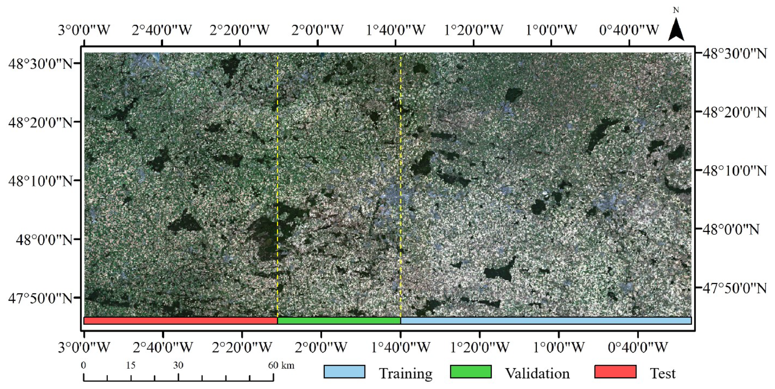
2.1. Study Area and Remote Sensing Data
2.2. Points Training Set
3. Methodology
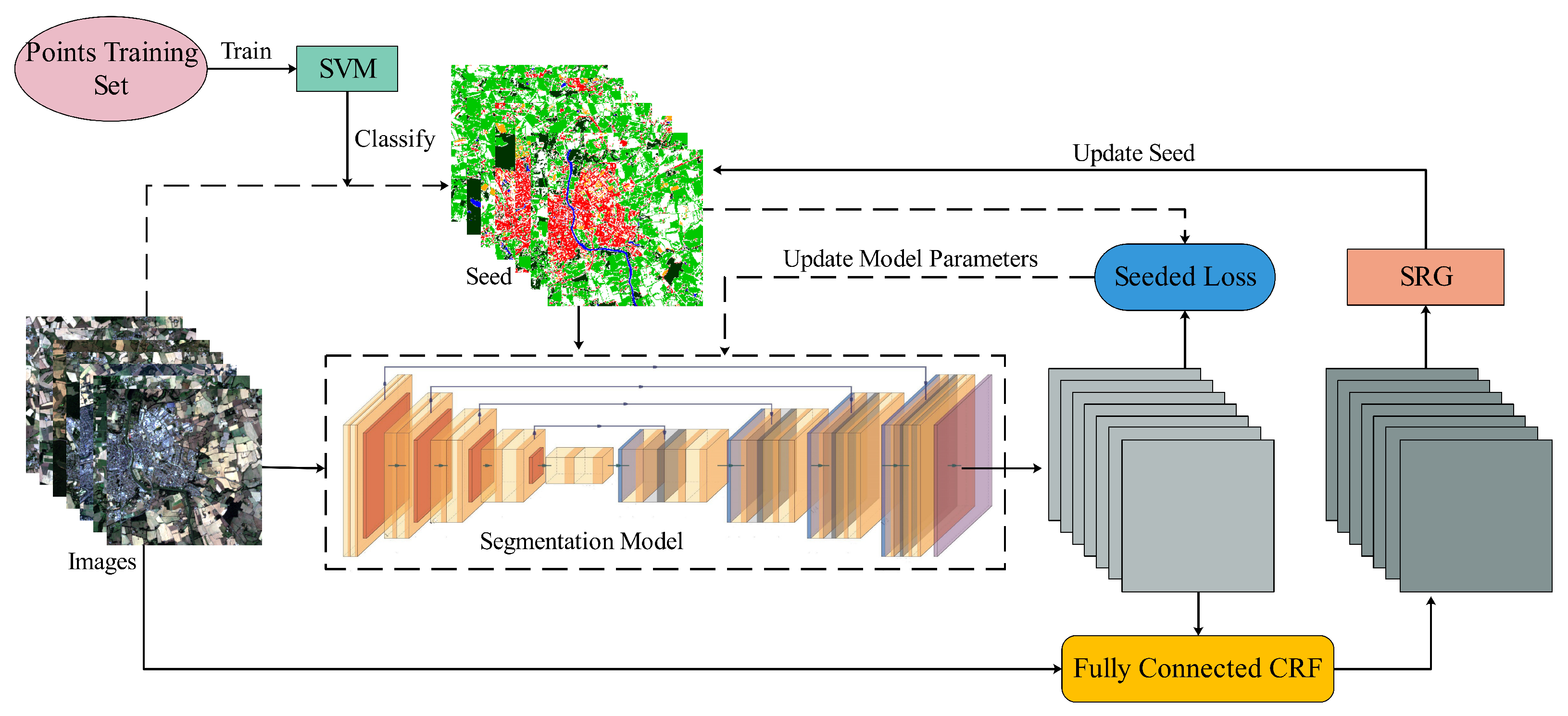
- (1)
- Initial seed generation: Use points training set (as described in Section 2.2) to generate the initial seeded pixel-level data set (denoted as seed) including training set and validation set using SVM, in which only confident points are treated as seed points.
- (2)
- Train the segmentation model: Use seed (seed when firstly training) to train the segmentation model, and seeded loss is used to update the model parameters.
- (3)
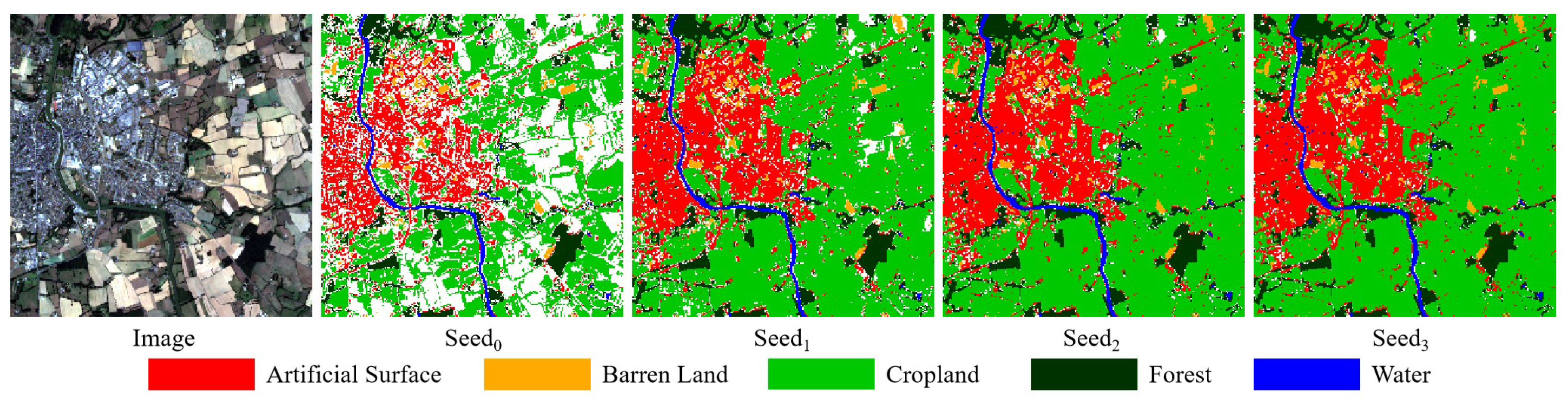
- Update seed: Take images of seed as the input of the fully trained segmentation model from Procedure (2) to produce the probability maps, then the fully connected CRF and SRG are used to update seed to get the updated seed based on the input images and output probability maps.
- (4)
- Iterate until convergence: Treat seed as a new data set to iterate Procedures (2) and (3) until seed points within the data set no longer change.
- (5)
- Classification stage: Use the final trained segmentation model to classify test images to get the classification results.
3.1. Initial Seed Generation Using Points Training Set
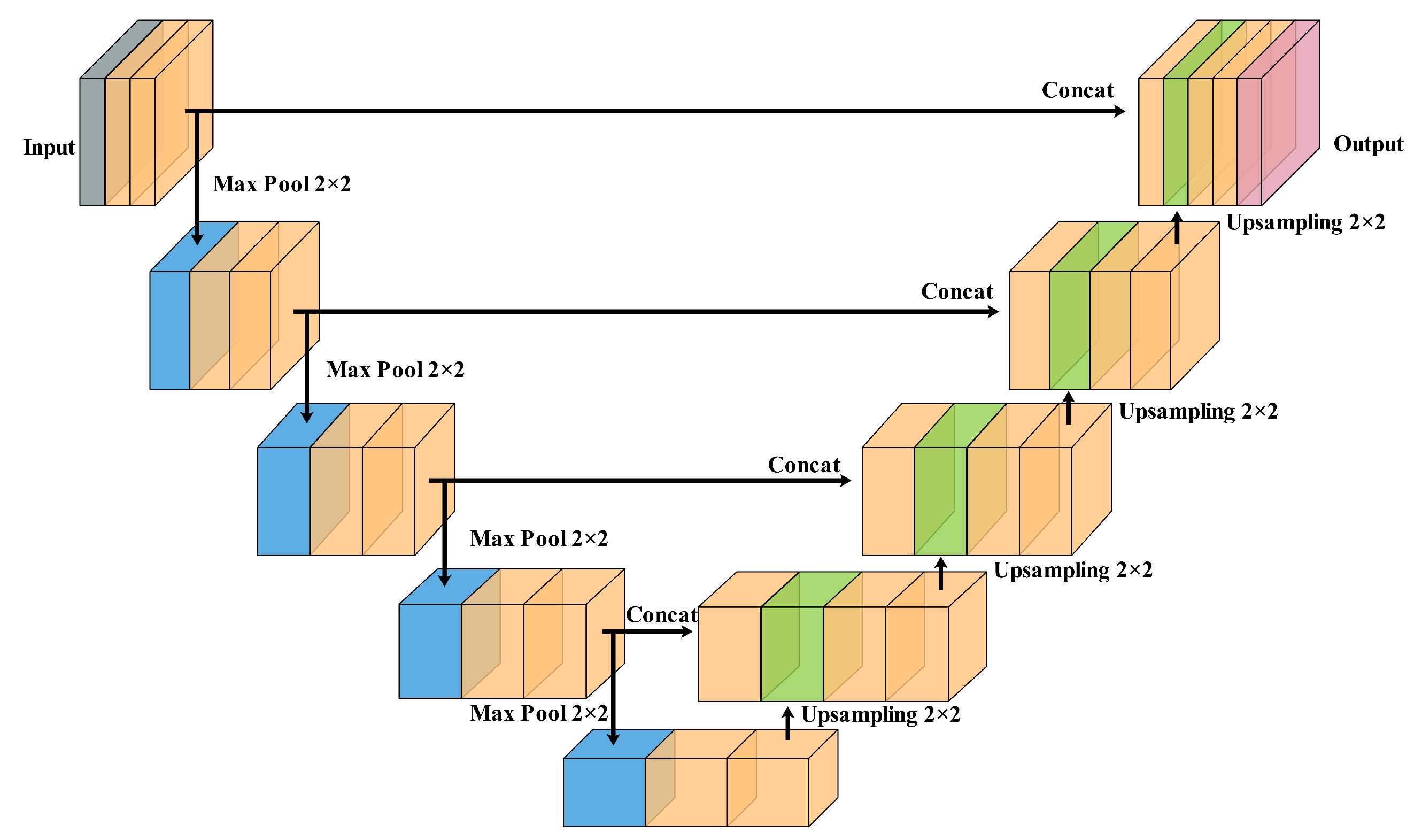
3.2. Semantic Segmentation Model
3.3. Seeded Loss
3.4. Fully Connected CRF
3.5. Seeded Region Growing (SRG)
4. Results and Analysis
4.1. Experimental Setup
4.1.1. Implement Details
4.1.2. Evaluation Metrics
4.1.3. Test Set
4.2. Experimental Results and Analysis
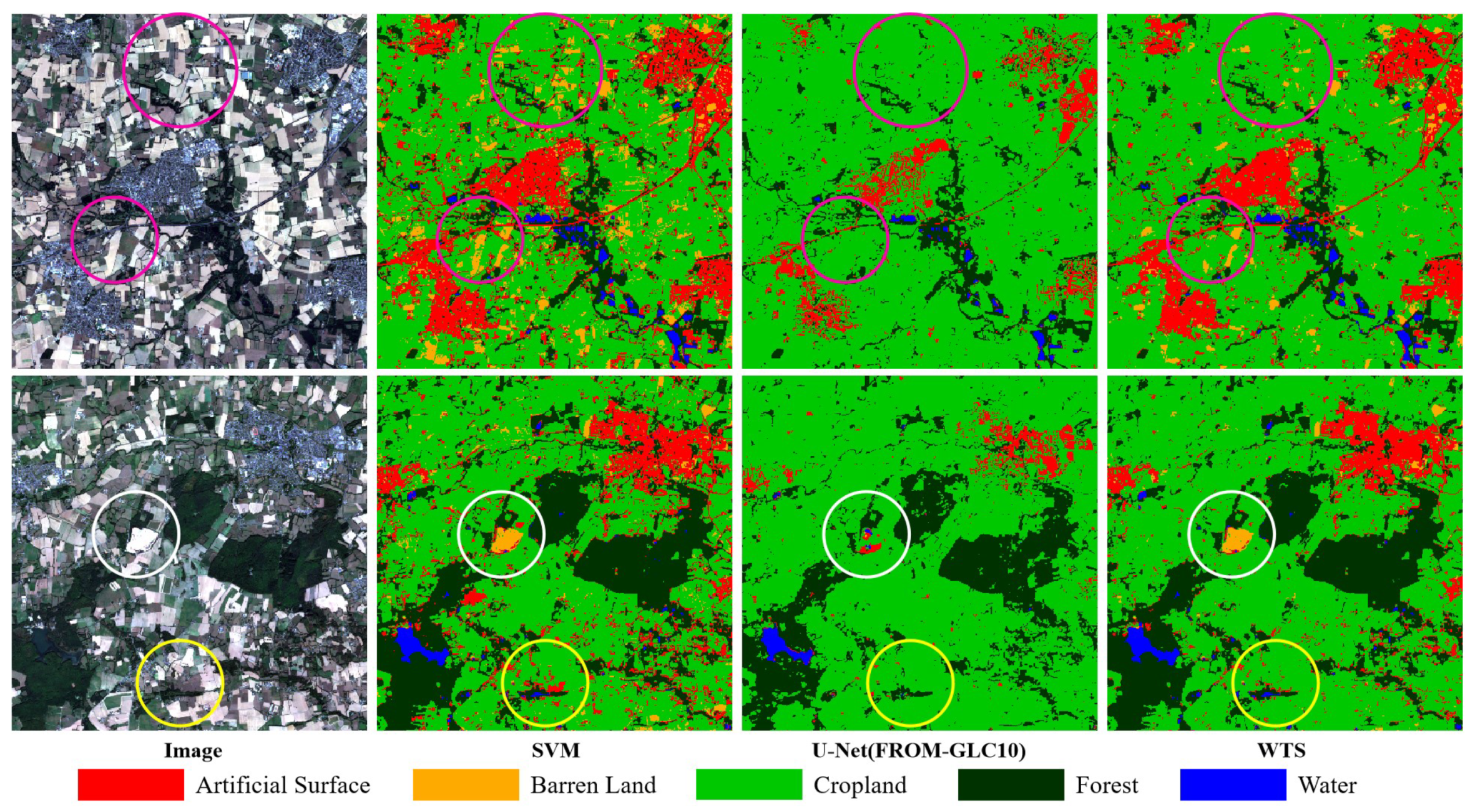
4.2.1. Results of WTS and Compared Methods
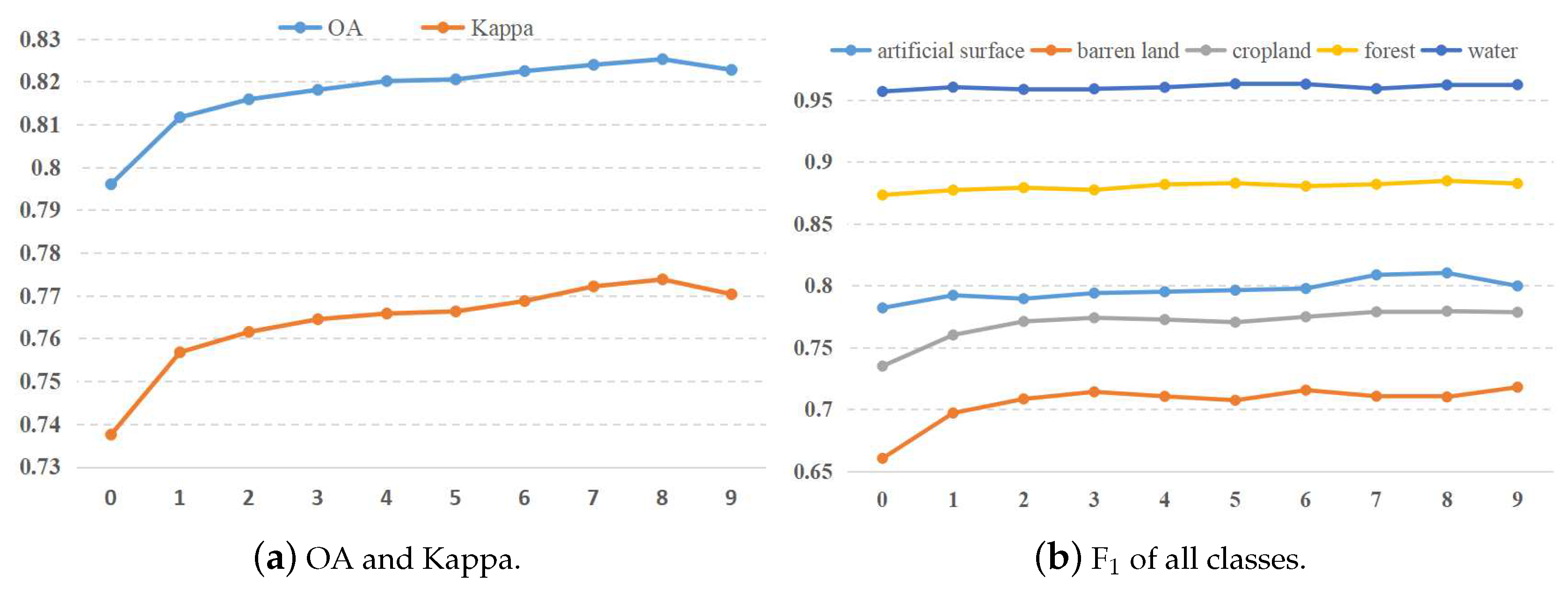
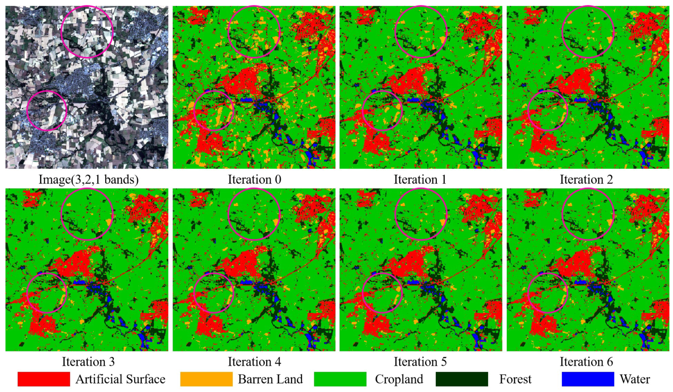
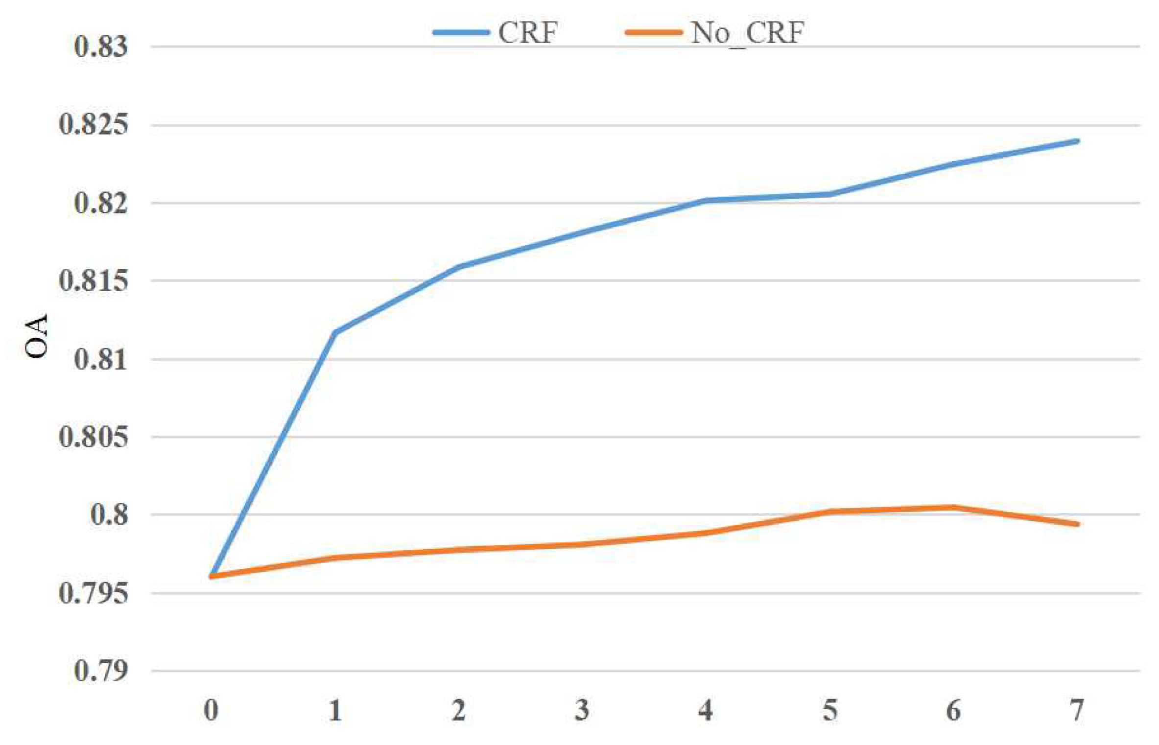
4.2.2. Results in Different Iterations of WTS
5. Discussion
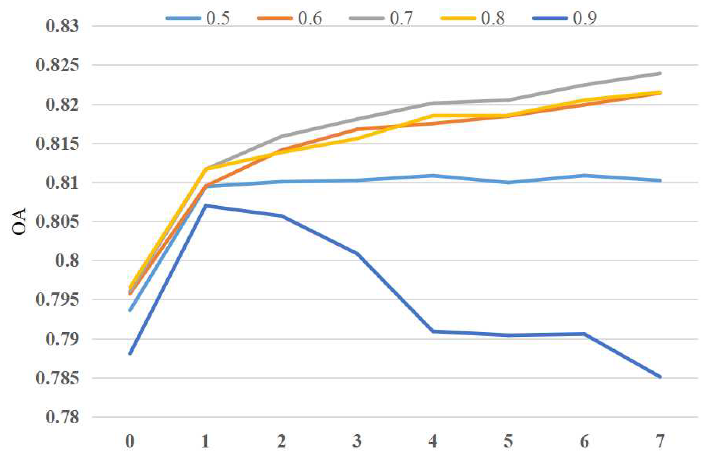
5.1. Influence of Probability Threshold to Generate Initial Seed on Classification Result
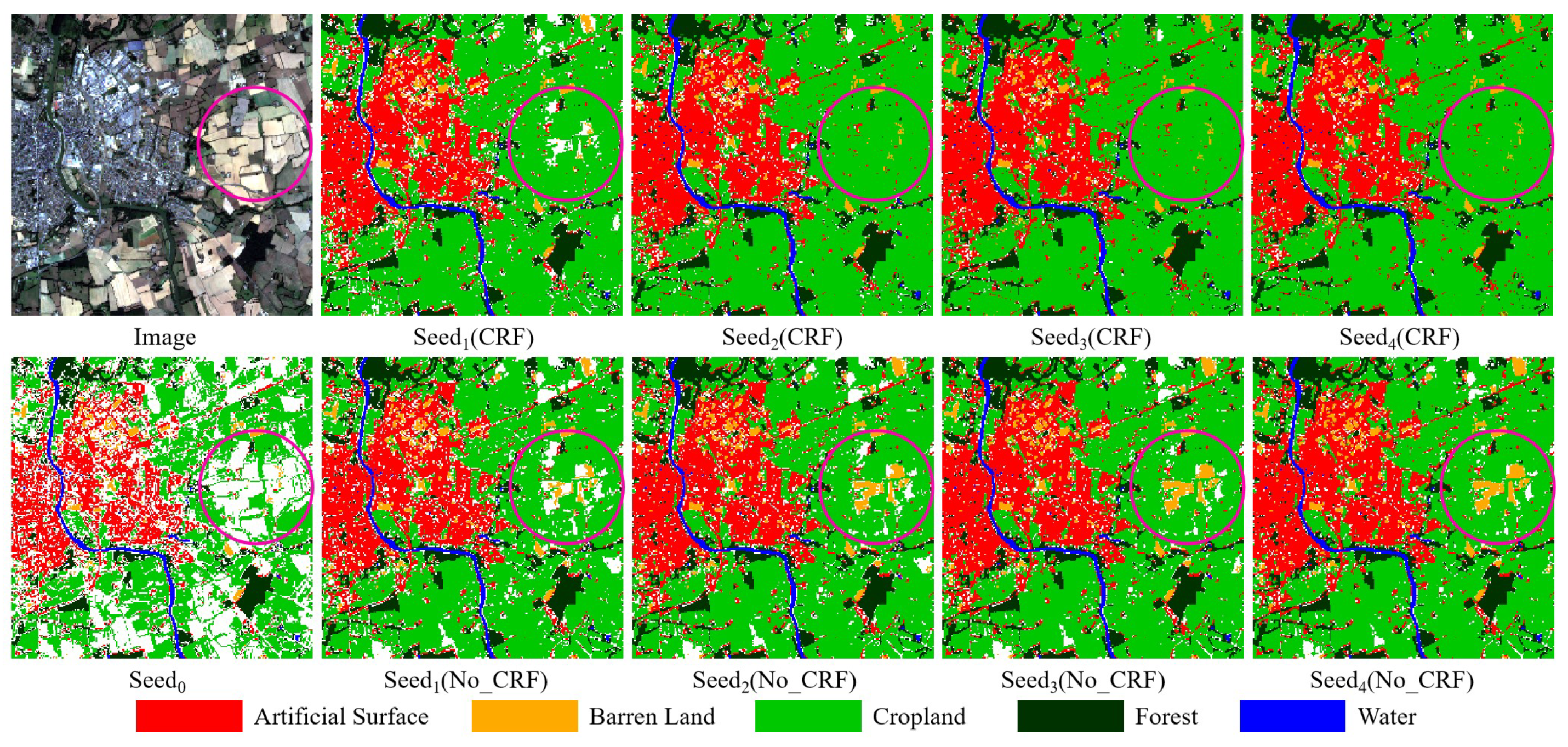
5.2. Influence of Fully Connected CRF on Classification Results
6. Conclusions and Future Work
Author Contributions
Funding
Institutional Review Board Statement
Informed Consent Statement
Acknowledgments
Conflicts of Interest
References
- Shi, H.; Chen, L.; Bi, F.; Chen, H.; Yu, Y. Accurate Urban Area Detection in Remote Sensing Images. IEEE Geosci. Remote Sens. Lett. 2015, 12, 1948–1952. [Google Scholar] [CrossRef]
- Kussul, N.; Lavreniuk, M.; Skakun, S.; Shelestov, A. Deep Learning Classification of Land Cover and Crop Types Using Remote Sensing Data. IEEE Geosci. Remote Sens. Lett. 2017, 14, 778–782. [Google Scholar] [CrossRef]
- Mountrakis, G.; Im, G.; Ogole, C. Support Vector Machines in Remote Sensing: A Review. ISPRS J. Photogramm. Remote Sens. 2011, 66, 247–259. [Google Scholar] [CrossRef]
- Phan, T.N.; Kuch, V.; Lehnert, L.W. Land Cover Classification Using Google Earth Engine and Random Forest Classifier—The Role of Image Composition. Remote Sens. 2020, 12, 2411. [Google Scholar] [CrossRef]
- Zhou, L.; Yang, X. Training Algorithm Performance for Image Classification by Neural Networks. Photogramm. Eng. Remote Sens. 2010, 76, 945–951. [Google Scholar] [CrossRef]
- He, K.; Zhang, X.; Ren, S.; Sun, J. Deep Residual Learning for Image Recognition. In Proceedings of the 2016 IEEE Conference on Computer Vision and Pattern Recognition, CVPR 2016, Las Vegas, NV, USA, 27–30 June 2016; pp. 770–778. [Google Scholar] [CrossRef] [Green Version]
- Girshick, R.B.; Donahue, J.; Darrell, T.; Malik, J. Rich Feature Hierarchies for Accurate Object Detection and Semantic Segmentation. In Proceedings of the 2014 IEEE Conference on Computer Vision and Pattern Recognition, CVPR 2014, Columbus, OH, USA, 23–28 June 2014; pp. 580–587. [Google Scholar] [CrossRef] [Green Version]
- Ren, S.; He, K.; Girshick, R.B.; Sun, J. Faster R-CNN: Towards Real-Time Object Detection with Region Proposal Networks. IEEE Trans. Pattern Anal. Mach. Intell. 2017, 39, 1137–1149. [Google Scholar] [CrossRef] [Green Version]
- Zhao, L.; Zhang, W.; Tang, P. Analysis of the Inter-Dataset Representation Ability of Deep Features for High Spatial Resolution Remote Sensing Image Scene Classification. Multimed. Tools Appl. 2019, 78, 9667–9689. [Google Scholar] [CrossRef]
- Zhang, W.; Tang, P.; Zhao, L. Remote Sensing Image Scene Classification Using CNN-CapsNet. Remote Sens. 2019, 11, 494. [Google Scholar] [CrossRef] [Green Version]
- Ma, D.; Tang, P.; Zhao, L. SiftingGAN: Generating and Sifting Labeled Samples to Improve the Remote Sensing Image Scene Classification Baseline In Vitro. IEEE Geosci. Remote Sens. Lett. 2019, 16, 1046–1050. [Google Scholar] [CrossRef] [Green Version]
- Wang, C.; Bai, X.; Wang, S.; Zhou, J.; Ren, P. Multiscale Visual Attention Networks for Object Detection in VHR Remote Sensing Images. IEEE Geosci. Remote Sens. Lett. 2019, 16, 310–314. [Google Scholar] [CrossRef]
- Chen, C.; Gong, W.; Chen, Y.; Li, W. Object Detection in Remote Sensing Images Based on A Scene-Contextual Feature Pyramid Network. Remote Sens. 2019, 11, 339. [Google Scholar] [CrossRef] [Green Version]
- Wang, Q.; Zhang, X.; Chen, G.; Dai, F.; Gong, Y.; Zhu, K. Change Detection Based on Faster R-CNN for High-Resolution Remote Sensing Images. Remote Sens. Lett. 2018, 9, 923–932. [Google Scholar] [CrossRef]
- Ji, S.; Shen, Y.; Lu, M.; Zhang, Y. Building Instance Change Detection from Large-Scale Aerial Images using Convolutional Neural Networks and Simulated Samples. Remote Sens. 2019, 11, 1343. [Google Scholar] [CrossRef] [Green Version]
- Mnih, V. Machine Learning for Aerial Image Labeling; University of Toronto: Toronto, ON, Canada, 2013. [Google Scholar]
- MahdianPari, M.; Salehi, B.; Rezaee, M.; Mohammadimanesh, F.; Zhang, Y. Very Deep Convolutional Neural Networks for Complex Land Cover Mapping Using Multispectral Remote Sensing Imagery. Remote Sens. 2018, 10, 1119. [Google Scholar] [CrossRef] [Green Version]
- Liu, T.; Abd-Elrahman, A.; Morton, J.; Wilhelm, V.L. Comparing Fully Convolutional Networks, Random forest, Support Vector Machine, and Patch-Based Deep Convolutional Neural Networks for Object-Based Wetland Mapping Using Images From Small Unmanned Aircraft System. GISci. Remote Sens. 2018, 55, 243–264. [Google Scholar] [CrossRef]
- Kwan, C.; Ayhan, B.; Budavari, B.; Lu, Y.; Perez, D.; Li, J.; Bernabe, S.; Plaza, A. Deep Learning for Land Cover Classification Using Only a Few Bands. Remote Sens. 2020, 12, 2000. [Google Scholar] [CrossRef]
- Pan, X.; Zhao, J. A Central-Point-Enhanced Convolutional Neural Network for High-Resolution Remote-Sensing Image Classification. Int. J. Remote Sens. 2017, 38, 6554–6581. [Google Scholar] [CrossRef]
- Maggiori, E.; Tarabalka, Y.; Charpiat, G.; Alliez, P. Convolutional Neural Networks for Large-Scale Remote-Sensing Image Classification. IEEE Trans. Geosci. Remote Sens. 2017, 55, 645–657. [Google Scholar] [CrossRef] [Green Version]
- Long, J.; Shelhamer, E.; Darrell, T. Fully Convolutional Networks for Semantic Segmentation. In Proceedings of the 2015 IEEE Conference on Computer Vision and Pattern Recognition, CVPR 2015, Boston, MA, USA, 7–12 June 2015; pp. 3431–3440. [Google Scholar] [CrossRef] [Green Version]
- Persello, C.; Stein, A. Deep Fully Convolutional Networks for the Detection of Informal Settlements in VHR Images. IEEE Geosci. Remote Sens. Lett. 2017, 14, 2325–2329. [Google Scholar] [CrossRef]
- Wang, H.; Wang, Y.; Zhang, Q.; Xiang, S.; Pan, C. Gated Convolutional Neural Network for Semantic Segmentation in High-Resolution Images. Remote Sens. 2017, 9, 446. [Google Scholar] [CrossRef] [Green Version]
- Sun, W.; Wang, R. Fully Convolutional Networks for Semantic Segmentation of Very High Resolution Remotely Sensed Images Combined with DSM. IEEE Geosci. Remote Sens. Lett. 2018, 15, 474–478. [Google Scholar] [CrossRef]
- Fu, G.; Liu, C.; Zhou, R.; Sun, T.; Zhang, Q. Classification for High Resolution Remote Sensing Imagery Using A Fully Convolutional Network. Remote Sens. 2017, 9, 498. [Google Scholar] [CrossRef] [Green Version]
- Gerke, M. Use of The Stair Vision Library Within The ISPRS 2D Semantic Labeling Benchmark (Vaihingen); ResearcheGate: Berlin, Germany, 2014. [Google Scholar] [CrossRef]
- Demir, I.; Koperski, K.; Lindenbaum, D.; Pang, G.; Huang, J.; Basu, S.; Hughes, F.; Tuia, D.; Raska, R. DeepGlobe 2018: A Challenge to Parse the Earth through Satellite Images. In Proceedings of the 2018 IEEE/CVF Conference on Computer Vision and Pattern Recognition Workshops (CVPRW), Salt Lake City, UT, USA, 18–22 June 2018; pp. 172–17209. [Google Scholar]
- Schmitt, M.; Hughes, L.H.; Qiu, C.; Zhu, X.X. SEN12MS–A Curated Dataset of Georeferenced Multi-Spectral Sentinel-1/2 Imagery for Deep Learning and Data Fusion. ISPRS Ann. Photogramm. Remote Sens. Spat. Inf. Sci. 2019, IV-2/W7, 153–160. [Google Scholar] [CrossRef] [Green Version]
- Xin-Yi, T.; Gui-Song, X.; Qikai, L.; Huanfeng, S.; Shengyang, L.; Shucheng, Y.; Liangpei, Z. Learning Transferable Deep Models for Land-Use Classification with High-Resolution Remote Sensing Images. arXiv 2018, arXiv:1807.05713. [Google Scholar]
- Isikdogan, F.; Bovik, A.C.; Passalacqua, P. Surface Water Mapping by Deep Learning. IEEE J. Sel. Topics Appl. Earth Observ. Remote Sens. 2017, 10, 4909–4918. [Google Scholar] [CrossRef]
- Feng, M.; Sexton, J.O.; Channan, S.; Townshend, J.R. A Global, High-Resolution (30-m) Inland Water Body Dataset for 2000: First Results of A Topographic-Spectral Classification Algorithm. Int. J. Digit. Earth 2016, 9, 113–133. [Google Scholar] [CrossRef] [Green Version]
- Scepanovic, S.; Antropov, O.; Laurila, P.; Ignatenko, V.; Praks, J. Wide-Area Land Cover Mapping with Sentinel-1 Imagery using Deep Learning Semantic Segmentation Models. arXiv 2019, arXiv:1912.05067. [Google Scholar]
- Chantharaj, S.; Pornratthanapong, K.; Chitsinpchayakun, P.; Panboonyuen, T.; Vateekul, P.; Lawavirojwong, S.; Srestasathiern, P.; Jitkajornwanich, K. Semantic Segmentation on Medium-Resolution Satellite Images Using Deep Convolutional Networks with Remote Sensing Derived Indices. In Proceedings of the 2018 15th International Joint Conference on Computer Science and Software Engineering (JCSSE), Nakhonpathom, Thailand, 11–13 July 2018; pp. 1–6. [Google Scholar]
- Grekousis, G.; Mountrakis, G.; Kavouras, M. An Overview of 21 Global and 43 Regional Land-Cover Mapping Products. Int. J. Remote Sens. 2015, 36, 5309–5335. [Google Scholar] [CrossRef]
- Ghosh, A.; Kumar, H.; Sastry, P. Robust Loss Functions under Label Noise for Deep Neural Networks. In Proceedings of the Thirty-First AAAI Conference on Artificial Intelligence, San Francisco, CA, USA, 4–9 February 2017. [Google Scholar]
- Sukhbaatar, S.; Bruna, J.; Paluri, M.; Bourdev, L.; Fergus, R. Training Convolutional Networks with Noisy Labels. arXiv 2014, arXiv:1406.2080. [Google Scholar]
- Han, B.; Yao, Q.; Yu, X.; Niu, G.; Xu, M.; Hu, W.; Tsang, I.; Sugiyama, M. Co-teaching: Robust Training of Deep Neural Networks with Extremely Noisy Labels. In Proceedings of the 2018 Neural Information Processing Systems, Montreal, QC, Canada, 2–8 December 2018; pp. 8535–8545. [Google Scholar]
- Mnih, V.; Hinton, G.E. Learning to Label Aerial Images from Noisy Data. In Proceedings of the 29th International conference on machine learning (ICML-12), Edinburgh, Scotland, 26 June–1 July 2012; pp. 567–574. [Google Scholar]
- Papandreou, G.; Chen, L.; Murphy, K.P.; Yuille, A.L. Weakly-and Semi-Supervised Learning of A Deep Convolutional Network for Semantic Image Segmentation. In Proceedings of the 2015 IEEE International Conference on Computer Vision, Santiago, Chile, 11–18 December 2015; pp. 1742–1750. [Google Scholar]
- Bearman, A.; Russakovsky, O.; Ferrari, V.; Fei-Fei, L. What’s the Point: Semantic Segmentation with Point Supervision. In Proceedings of the 2016 European Conference on Computer Vision, Amsterdam, The Netherlands, 8–16 October 2016; pp. 549–565. [Google Scholar]
- Dai, J.; He, K.; Sun, J. Boxsup: Exploiting Bounding Boxes to Supervise Convolutional Networks for Semantic Segmentation. In Proceedings of the 2015 IEEE International Conference on Computer Vision, Santiago, Chile, 11–18 December 2015; pp. 1635–1643. [Google Scholar]
- Lin, D.; Dai, J.; Jia, J.; He, K.; Sun, J. Scribblesup: Scribble-Supervised Convolutional Networks for Semantic Segmentation. In Proceedings of the IEEE Conference on Computer Vision and Pattern Recognition, CVPR 2016, Las Vegas, NV, USA, 27–30 June 2016; pp. 3159–3167. [Google Scholar]
- Chan, L.; Hosseini, M.S.; Plataniotis, K.N. A Comprehensive Analysis of Weakly-Supervised Semantic Segmentation in Different Image Domains. arXiv 2019, arXiv:1912.11186. [Google Scholar] [CrossRef]
- Fu, K.; Lu, W.; Diao, W.; Yan, M.; Sun, H.; Zhang, Y.; Sun, X. WSF-NET: Weakly Supervised Feature-Fusion Network for Binary Segmentation in Remote Sensing Image. Remote Sens. 2018, 10, 1970. [Google Scholar] [CrossRef] [Green Version]
- Zhang, L.; Ma, J.; Lv, X.; Chen, D. Hierarchical Weakly Supervised Learning for Residential Area Semantic Segmentation in Remote Sensing Images. IEEE Geosci. Remote Sens. Lett. 2019, 17, 117–121. [Google Scholar] [CrossRef]
- Adams, R.; Bischof, L. Seeded Region Growing. IEEE Trans. Pattern Anal. Mach. Intell. 1994, 16, 641–647. [Google Scholar] [CrossRef] [Green Version]
- Badrinarayanan, V.; Kendall, A.; Cipolla, R. SegNet: A Deep Convolutional Encoder-Decoder Architecture for Image Segmentation. IEEE Trans. Pattern Anal. Mach. Intell. 2017, 39, 2481–2495. [Google Scholar] [CrossRef] [PubMed]
- Chen, L.; Papandreou, G.; Kokkinos, I.; Murphy, K.; Yuille, A.L. DeepLab: Semantic Image Segmentation with Deep Convolutional Nets, Atrous Convolution, and Fully Connected CRFs. IEEE Trans. Pattern Anal. Mach. Intell. 2018, 40, 834–848. [Google Scholar] [CrossRef] [PubMed]
- Ronneberger, O.; Fischer, P.; Brox, T. U-Net: Convolutional Networks for Biomedical Image Segmentation. In Proceedings of the Medical Image Computing and Computer-Assisted Intervention—MICCAI 2015—18th International Conference, Munich, Germany, 5–9 October 2015; Proceedings, Part III. pp. 234–241. [Google Scholar] [CrossRef] [Green Version]
- Simon, J.; Michal, D.; David, V.; Adriana, R.; Yoshua, B. The One Hundred Layers Tiramisu: Fully Convolutional Densenets for Semantic Segmentation. In Proceedings of the IEEE Conference on Computer Vision and Pattern Recognition Workshops, Honolulu, HI, USA, 21–26 July 2017; pp. 11–19. [Google Scholar]
- Kolesnikov, A.; Lampert, C.H. Seed, Expand and Constrain: Three Principles for Weakly-Supervised Image Segmentation. In Proceedings of the 2016 European Conference on Computer Vision, Amsterdam, The Netherlands, 8–16 October 2016; pp. 695–711. [Google Scholar]
- Krähenbühl, P.; Koltun, V. Efficient Inference in Fully Connected CRFs with Gaussian Edge Potentials. In Proceedings of the 2011 Neural Information Processing Systems, Granada, Spain, 12–17 December 2011; pp. 109–117. [Google Scholar]
- Chih-Wei, H.; Chih-Chung, C.; Chih-Jen, L. A Practical Guide to Support Vector Classification. BJU Int. 2008, 101, 1396–1400. [Google Scholar]
- Gong, P.; Liu, H.; Zhang, M.; Li, C.; Wang, J.; Huang, H.; Clinton, N.; Ji, L.; Li, W.; Bai, Y.; et al. Stable Classification with Limited Sample: Transferring A 30-m Resolution Sample Set Collected in 2015 to Mapping 10-m Resolution Global Land Cover in 2017. Sci. Bull. 2019, 64, 370–373. [Google Scholar] [CrossRef] [Green Version]


| Band Number | Spectral Region | Central Wavelength (nm) | Bandwidth (nm) | Spatial Resolution (m) |
|---|---|---|---|---|
| 2 | Blue | 492.1 | 98 | 10 |
| 3 | Green | 559 | 46 | 10 |
| 4 | Red | 665 | 39 | 10 |
| 5 | Vegetation Red Edge | 703.8 | 20 | 20 |
| 6 | Vegetation Red Edge | 739.1 | 18 | 20 |
| 7 | Vegetation Red Edge | 779.7 | 28 | 20 |
| 8 | NIR | 833 | 133 | 10 |
| 8a | Vegetation Red Edge | 864 | 32 | 20 |
| 11 | SWIR | 1610.4 | 141 | 20 |
| 12 | SWIR | 2185.7 | 238 | 20 |
| Class | Short Description | Number of Points | Area (km) |
|---|---|---|---|
| Artificial Surface | Artificial covers such as urban areas, rural cottages and roads. | 3332 | 1.3328 |
| Barren Land | Surface vegetation is hardly observable, such as urban areas with little constructed material, bare mines and beaches. | 3309 | 1.3236 |
| Cropland | Human planted land that generally has regular distribution patterns including cultivated land and fallow land. | 3726 | 1.4904 |
| Forest | Trees observable in the landscape, such as broadleaf forest, needleleaf forest and shrubland | 3467 | 1.3868 |
| Water | Water bodies such as rivers, lakes, reservoirs and ponds. | 3010 | 1.2040 |
| Artificial Surface | Barren Land | Cropland | Forest | Water | OA | Kappa | |
|---|---|---|---|---|---|---|---|
| SVM | 0.7879 | 0.6492 | 0.7391 | 0.8689 | 0.9480 | 0.7965 | 0.7377 |
| /0.6501 | /0.4806 | /0.5861 | /0.7681 | /0.9012 | |||
| U-Net(FROM-GLC10) | 0.5513 | 0.0070 | 0.7365 | 0.8602 | 0.8928 | 0.6943 | 0.5919 |
| /0.3801 | /0.0035 | /0.5829 | /0.7547 | /0.8064 | |||
| WTS | 0.8103 | 0.7100 | 0.7793 | 0.8847 | 0.9623 | 0.8252 | 0.7738 |
| /0.6810 | /0.5503 | /0.6384 | /0.7932 | /0.9273 |
| Probability Threshold | Unlabeled | Artificial Surface | Barren Land | Cropland | Forest | Water |
|---|---|---|---|---|---|---|
| 0.5 | 6.14 | 8.63 | 3.62 | 61.55 | 19.06 | 1.01 |
| 0.6 | 18.70 | 6.20 | 2.22 | 55.67 | 16.26 | 0.95 |
| 0.7 | 31.32 | 4.10 | 0.95 | 49.39 | 13.35 | 0.90 |
| 0.8 | 45.20 | 2.06 | 0.39 | 41.37 | 10.14 | 0.84 |
| 0.9 | 63.32 | 0.14 | 0.17 | 28.99 | 6.64 | 0.74 |
Publisher’s Note: MDPI stays neutral with regard to jurisdictional claims in published maps and institutional affiliations. |
© 2021 by the authors. Licensee MDPI, Basel, Switzerland. This article is an open access article distributed under the terms and conditions of the Creative Commons Attribution (CC BY) license (http://creativecommons.org/licenses/by/4.0/).
Share and Cite
Zhang, W.; Tang, P.; Corpetti, T.; Zhao, L. WTS: A Weakly towards Strongly Supervised Learning Framework for Remote Sensing Land Cover Classification Using Segmentation Models. Remote Sens. 2021, 13, 394. https://0-doi-org.brum.beds.ac.uk/10.3390/rs13030394
Zhang W, Tang P, Corpetti T, Zhao L. WTS: A Weakly towards Strongly Supervised Learning Framework for Remote Sensing Land Cover Classification Using Segmentation Models. Remote Sensing. 2021; 13(3):394. https://0-doi-org.brum.beds.ac.uk/10.3390/rs13030394
Chicago/Turabian StyleZhang, Wei, Ping Tang, Thomas Corpetti, and Lijun Zhao. 2021. "WTS: A Weakly towards Strongly Supervised Learning Framework for Remote Sensing Land Cover Classification Using Segmentation Models" Remote Sensing 13, no. 3: 394. https://0-doi-org.brum.beds.ac.uk/10.3390/rs13030394