A Dual-Model Architecture with Grouping-Attention-Fusion for Remote Sensing Scene Classification


1
Unmanned System Research Institute, Northwestern Polytechnical University, Xi’an 710072, China
2
National Pilot School of Software, Yunnan University, Kunming 650504, China
3
Center for OPTical IMagery Analysis and Learning (OPTIMAL), Northwestern Polytechnical University, Xi’an 710072, China
4
School of Electronics and Information, Northwestern Polytechnical University, Xi’an 710072, China
*
Author to whom correspondence should be addressed.
Remote Sens. 2021, 13(3), 433; https://0-doi-org.brum.beds.ac.uk/10.3390/rs13030433
Submission received: 25 December 2020
/
Revised: 19 January 2021
/
Accepted: 21 January 2021
/
Published: 26 January 2021
Abstract
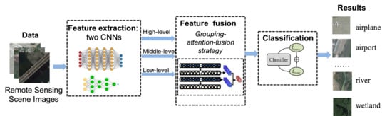
:Remote sensing images contain complex backgrounds and multi-scale objects, which pose a challenging task for scene classification. The performance is highly dependent on the capacity of the scene representation as well as the discriminability of the classifier. Although multiple models possess better properties than a single model on these aspects, the fusion strategy for these models is a key component to maximize the final accuracy. In this paper, we construct a novel dual-model architecture with a grouping-attention-fusion strategy to improve the performance of scene classification. Specifically, the model employs two different convolutional neural networks (CNNs) for feature extraction, where the grouping-attention-fusion strategy is used to fuse the features of the CNNs in a fine and multi-scale manner. In this way, the resultant feature representation of the scene is enhanced. Moreover, to address the issue of similar appearances between different scenes, we develop a loss function which encourages small intra-class diversities and large inter-class distances. Extensive experiments are conducted on four scene classification datasets include the UCM land-use dataset, the WHU-RS19 dataset, the AID dataset, and the OPTIMAL-31 dataset. The experimental results demonstrate the superiority of the proposed method in comparison with the state-of-the-arts.
1. Introduction
The rapid development of satellites enables the acquisition of high-resolution remote sensing images which are consistently increasing in number. Compared with the low-resolution remote sensing images, the high-resolution images offer rich and detailed geographic information which is valuable in the fields of agriculture, military, geology, and atmosphere. At the same time, this advantage posts the requirement of scene understanding which is to label the images with semantic tags based on the image content and then facilitate the automatic analysis of remote sensing images. Targeting at this, scene classification [1,2,3,4,5] has already been a popular research topic and has witnessed successful deployment in related applications.
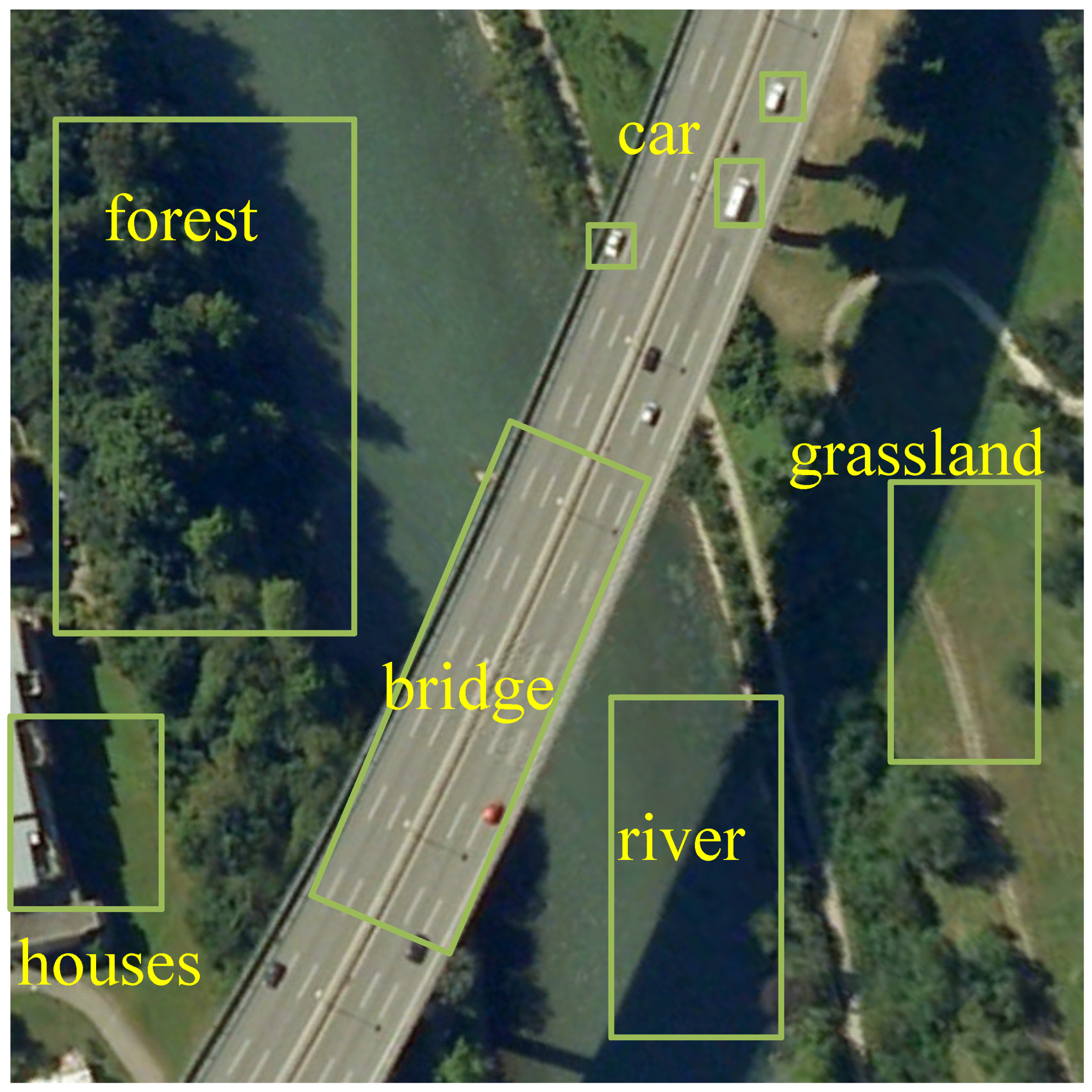
A remote sensing image typically covers a large range of lands, in which many kinds of objects exist, such as bridge, car, pond, forest, and grassland, as shown in Figure 1. This increases the difficulty of scene classification since the label of the scene could be ambiguous with respect to the primary object and the secondary objects. Hence, the feature representation of the image is the key factor that determines the performance of remote sensing scene classification. In an ideal case, the feature representation is expected to be highly correlated with the primary object, and less correlated with the secondary objects. Conventionally, hand-crafted features have been well studied to improve the classification accuracy, including global features (e.g., colors, textures, and GIST) and local features (e.g., SIFT, BovW, and LDA). However, these features do not have sufficient representation capacity and could not be adapted to kinds of scenes, which seriously limit the performance of scene classification. With the development of parallel computing, this bottleneck has been broken by the deep learning tools. The convolutional neural network (CNN) is a powerful model for analyzing image contents, which provides strong ability of hierarchical feature extraction. The deep CNN models including AlexNet [6], VGG-Net [7], ResNet [8], and DenseNet [9] have achieved impressive results on different vision tasks such as image classification and object detection. Benefiting from the advantages of CNN, the performance of scene classification is also improved by integrating the deep features and the remote sensing characteristics [10,11].
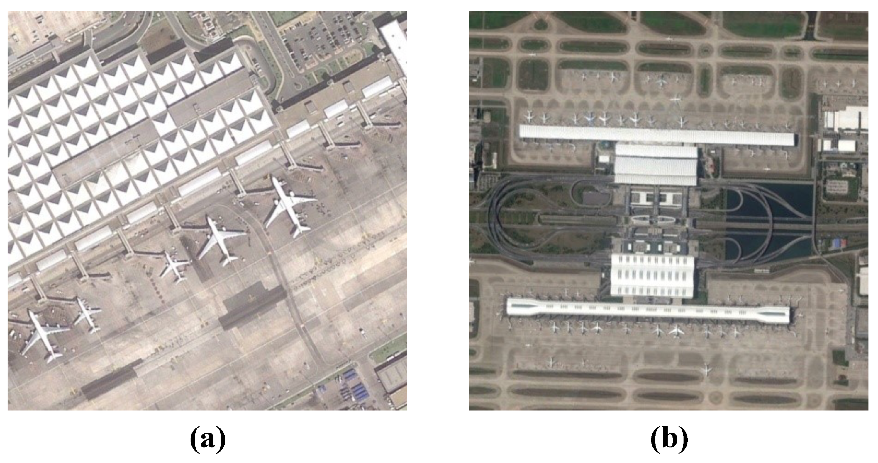
Considering that the remote sensing images are captured at different distances and the objects on lands have different sizes, the scales of the objects in the scene vary greatly. For example, as shown in Figure 2, the scenes of these two images are both labeled as “plane”, whereas the sizes of the planes in these figures are clearly different. It is expected that the feature representation of a model is robust on such a scale variation, such that the resultant features of the planes are similar to each other. Although the CNN models produce feature maps with different receptive field sizes, the features in shallow layers have strong discrimination ability for small objects and those in deep layers have strong discrimination ability for large objects. Unfortunately, most of existing methods only count on a single-level layer which is generally the last layer of the CNN model. This may result in the loss of the features of small objects, and hence is not suitable for the classification of multi-scale objects.
In the feature modelling process by CNN, the features of all channels in a layer have a complex heterogeneous distribution expressing similar concepts between different objects, such as appearance, shape, color, and semantics. This increases the difficulty of classification since the resultant features may be indistinguishable in the feature space. To alleviate this issue, the feature representation could be elaborated on different channels such that the feature space can be well constrained. Meanwhile, in scene classification, the label is mainly determined by the primary object in the scene. Hence, it is necessary to correlate the model features with the primary object and suppress the influence of the features of the secondary objects and the backgrounds.
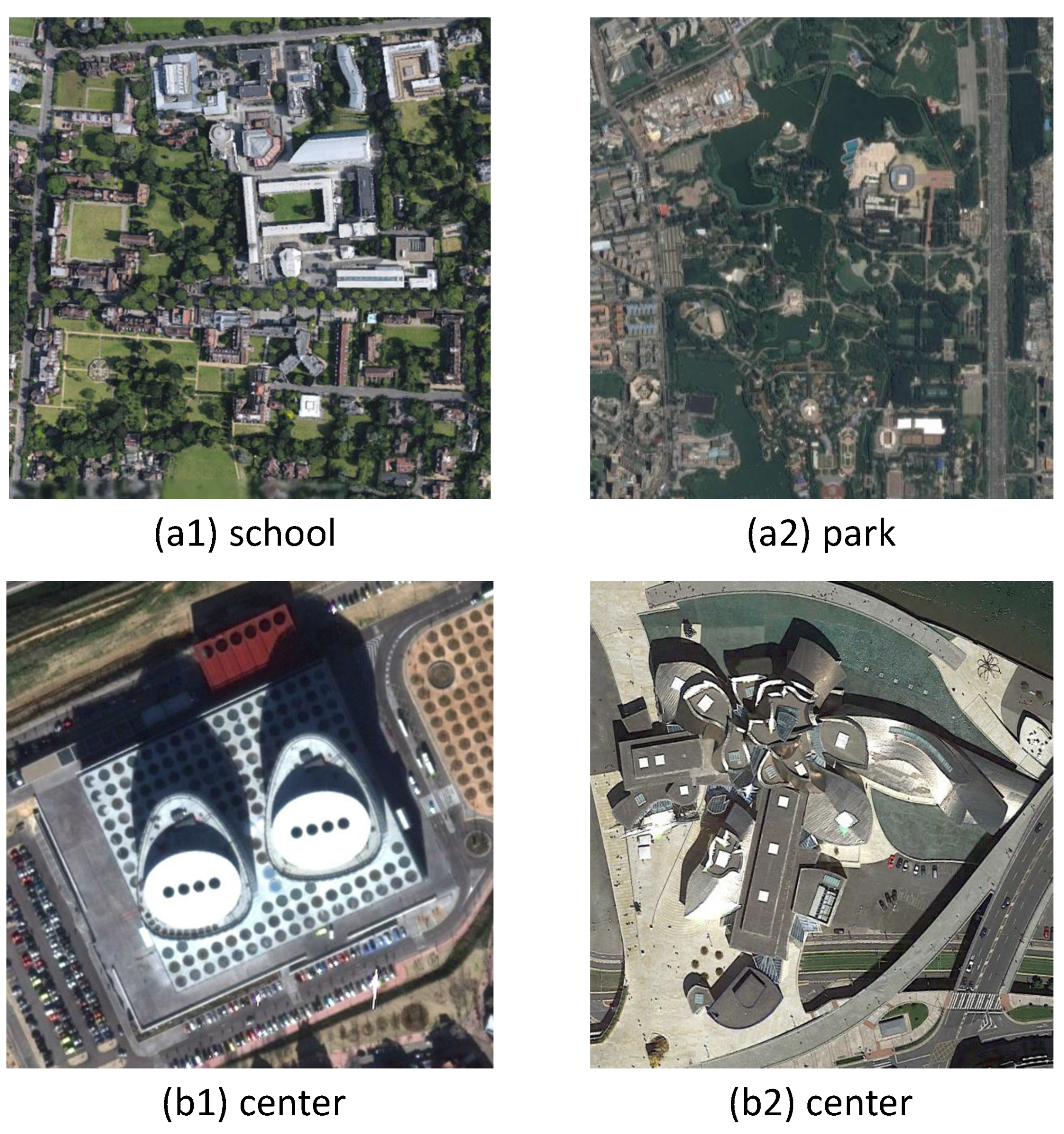
Moreover, the characteristics of remote sensing images state that the scenes have large intra-class diversity and large inter-class similarity. From Figure 3a, it can be seen that the school and the park have similar appearance, whereas from Figure 3b, both centers exhibit different building architectures in visualization. Although deep learning could greatly improve the classification performance by involving large amounts of training data, it has insufficient distinguishing ability for the remote sensing data with the above characteristics. This motivates us to explicitly constrain the intra-class diversity and inter-class similarity in the training objective by using, such as metric learning [12].
Based on the above idea, in this paper, we propose a novel dual-model architecture for the scene classification of remote sensing images. Specifically, we advocate that a single CNN model has limited feature representation capacity and hence, employ a dual-model architecture that integrates two different CNN models such that the advantages of two models can be exploited and fused. In the fusion process of two models, we develop a novel grouping-attention-fusion strategy, which implements a channel grouping mechanism followed by a spatial attention mechanism. This strategy is conducted on different feature levels of the two models, including low-level, middle-level, and high-level feature maps. The resultant features of the models in different scales are then fused using an elaborated schema. To improve the discrimination ability of the model, we improve the training loss by minimizing the intra-class diversities and maximizing inter-class distances. Extensive experiments are conducted on public datasets, and the results demonstrate the superiority of the proposed model compared with the state-of-the-arts. The contributions of this paper are summarized as follows:
- We propose a novel dual-model architecture to boost the performance of remote sensing scene classification, which compensates for the deficiency of a single CNN model in feature extraction.
- An improved loss function is proposed for training, which can alleviate the issue of high intra-class diversity and high inter-class similarity in remote sensing data.
- Extensive experimental results demonstrate the state-of-the-art performance of the proposed model.
2. Related Work
In this section, we briefly review the related work of remote sensing scene classification. The existing methods could be divided into two categories: the hand-crafted methods [1,13,14,15,16,17,18,19,20] and the deep learning-based methods [3,21,22,23,24,25,26,27,28,29,30,31,32].
2.1. The Hand-Crafted Methods
The hand-crafted feature extraction is a conventional way for representing the remote sensing images in scene classification. The global features [1,4,9,13,16,17,18] including the spectral characters, the color moment, the textures, and the shape descriptors, represent the image statistics from a whole view of the scene. However, the resultant statistics cannot reveal the local details of the scene, resulting in misclassification when the scenes have similar appearances. Instead, the local features such as SIFT [33] and HOG [1,17,18], describe the image in each local region, and mid-level descriptors are needed to compute the statistics of these local features. As for the requirement of performance improvement, the design of the hand-crafted features is getting more sophisticated, for example, combining different features to general a powerful one [19,34,35]. Zhu et al. [35] proposed the local-global feature as a visual bag of words for scene representation, which could fuse multiple features at histogram-level. Although multiple features can compensate the shortage of each individual feature, how to make an effective fusion by different types of features is still an open issue. Although the hand-crafted features do not rely on large-scale data and have low computation cost, the representation capacity is limited and cannot provide sufficient discrimination ability for the complex scenes, hence generally leading to unsatisfactory performance.
2.2. The Deep Learning-Based Methods
Benefiting from the development of high-performance computers and the availability of large-scale training data [36,37], deep learning-based approaches [38,39,40,41] have attracted more and more attention. Among the typical deep architectures, CNN provides a strong ability of feature extraction and yield significant performance improvement on scene classification. There have already been several attempts to use deep CNN features for classifying the remote sensing images [3,4,5,21,42,43,44,45,46,47]. Wang et al. [26] employed CaffeNet with the soft-max layer for scene classification. AlexNet incorporated with the extreme learning machine (ELM) classifier was used in [44]. To improve the feature representation, the attention mechanism is also integrated into CNN. Guo et al. [48] proposed a global-local attention network (GLANet) to obtain both global and local feature presentation for aerial scene classification. Wang et al. [49] proposed a residual attention network (RAN) by stacking various attention modules to capture attention perception features. Xiong et al. [50] proposed a novel attention module that could be integrated with the last feature layer of any pre-trained CNN model, such that the dominant features were enhanced through both spatial and channel attention. Zhao et al. [51] developed a multitask learning framework that improved the discrimination ability of the model features by taking advantage of different tasks. Kalajdjieski et al. [41] applied a series of deep CNNs together with other sensor data for the classification of air pollution.
More recently, multifeature fusion is considered in the design of CNN architectures to generate robust feature representation, which could yield performance improvement [1,13,14,23,31,52,53,54]. Drawing the thoughts of BovW, Huang et al. [14] proposed a CNN-based BovW feature for scene classification, which fused the features of the convolutional layers by BovW. Cheng et al. [1] extracted two features from CaffeNet and VGGNet, respectively, by fusing the features of the convolutional layer and the fully connected layer, which are then linearly combined for feature fusion. Shao et al. [53] explored two convolutional neural networks for feature extraction, which are fused. Cheng et al. [12] proposed the D-CNN model optimized by a new discriminative loss function which enforced the model to be more discriminative via a metric learning regularization. Yu et al. [55] designed a two-stream architecture for aerial scene classification. A feature fusion strategy based on multiple well pre-trained models was proposed by Petrovska et al. [56], which applied the principal component analysis on different layers of different models to produce multiple features that were then used for classification. He et al. [57] proposed a multilayer stacked covariance pooling method (MSCP) for scene classification, which computed the second-order features of the stacked feature maps extracted from multiple layers of a CNN model. The covariance pooling features could capture the fine-grained distortions among the small-scale objects in remote sensing images, thus producing improved performance. A similar technique was proposed by Akodad et al. [58], which assembled the second-order local and global features computed by covariance pooling. Zhang et al. [59] employed a fusion network for combining the shallow and deep features of CNN in the task of ship detection.
Although the models mentioned above have achieved great success in scene classification and other remote sensing tasks, they usually operate on the whole feature channel which has a complex inhomogeneous distribution. An elaborate passway and feature selection among the features could further improve the performance, which is the target of this paper.
3. The Proposed Method
In this section, we propose a novel and efficient dual-model architecture with deep feature fusion for remote sensing scene classification. Specifically, the whole model is composed of three components including a dual-model architecture for feature extraction, a grouping-attention-fusion strategy, and a metric learning-based loss function for optimization, which are introduced in the following.
3.1. The Dual-Model Architecture
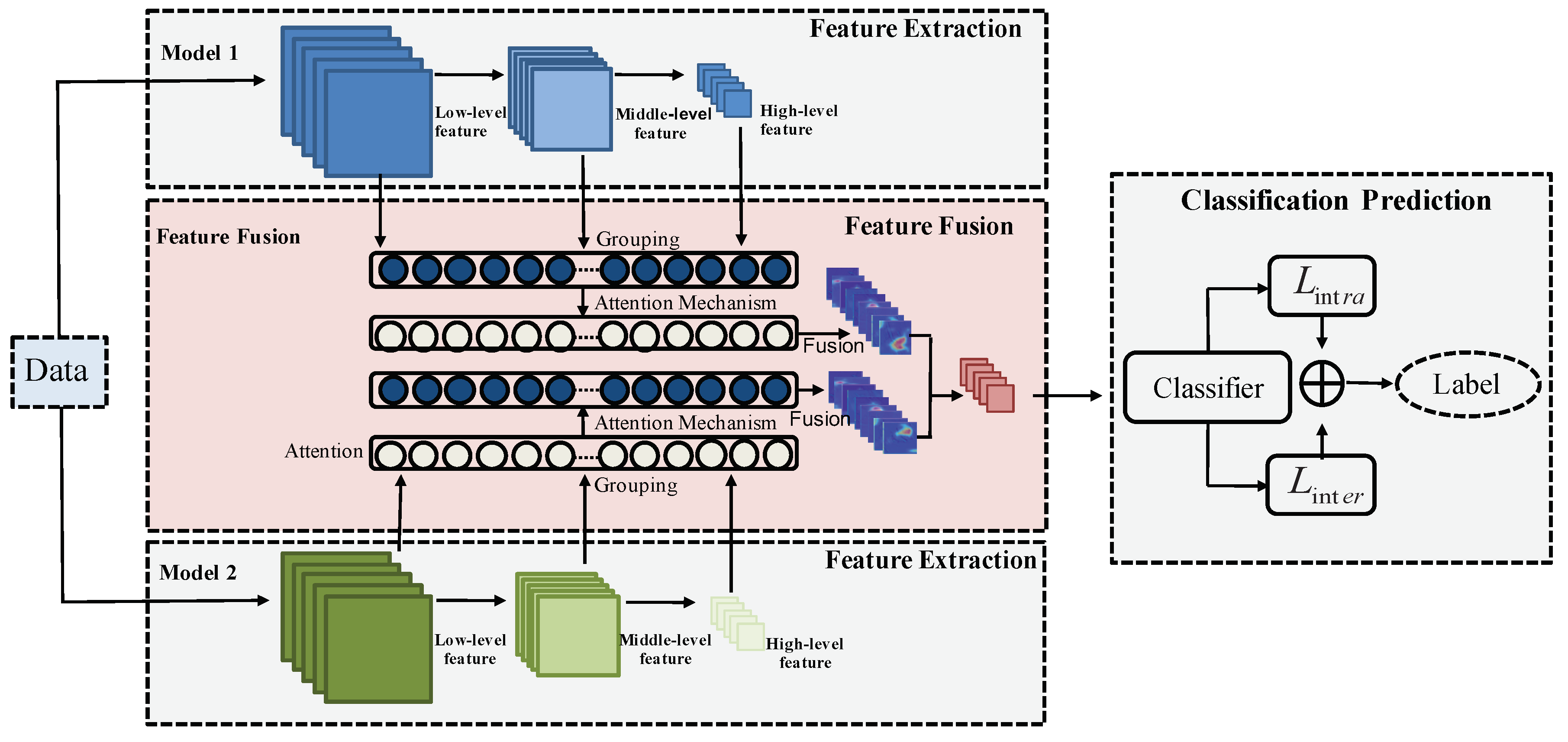
Different network architectures prefer to extract different types of features from the input image. Although those features may have redundant information, the complementary property of the features could be a key to improve the performance. At this regard, we propose a dual-model architecture to compensate the deficiency of a single model, which is illustrated in Figure 4. In each model of the dual models, features are extracted from multi-level layers including low-level, middle-level, and high-level features. The features of the corresponding layers are fused based on a grouping-attention-fusion strategy, which enhances the representation discrimination of the multi-scale objects in remote sensing images. The fused features of three levels are combined to yield the final multi-level feature, which is then fed to a loss function that enforces constraints on both intra-class diversity and inter-class similarity.
Regarding the dual models, we select two popular CNN models: ResNet [8] and DenseNet [9], for feature extraction, and each model is described in the following.
- ResNetResNet [8] is the most popular CNN for feature extraction, which solves the problem that the classification accuracy decreases by deepening the number of layers in some common CNNs. The lowest layer cannot only obtain the input from the middle layer, but also can obtain the input from the top layer through shortcut connection, which has the benefit of avoiding gradient vanishing. Although the network has an increased depth, it can easily enjoy accuracy gains. In our work, ResNet-50 is used for feature extraction, where we select the conv-2 layer for low-level feature extraction, the conv-3 layer for middle-level feature extraction, and the conv-4 layer for high-level feature extraction. These three layers produce features of 128 dimensions, 128 dimensions, and 128 dimensions, respectively.
- DenseNetCompared with other networks, DenseNet [9] alleviates gradient vanishing, strengthens feature propagation, encourages feature reusing, and reduces the number of parameters. A novel connectivity is proposed by DenseNet to make the information flow from low-level layers to high-level layers. Each layer obtains the input from all preceding layers and the resultant features are then transferred to subsequent layers. Consequently, both the low-level features and the high-level semantic features are used for final decision. In our architecture, we use DenseNet-121 as the feature extractor by extracting multi-level features from the conv-2 layer as the low-level feature with 128 dimensions, from the conv-3 layer as the middle-level feature with 128 dimensions, and from the conv-4 layer as the high-level feature with 128 dimensions.
3.2. Grouping-Attention-Fusion
The features extracted by the above CNN models are suitable for general purpose of image analysis, whereas scene classification focuses on the primary object in the scene. Considering this, the features could be further improved to enhance the discrimination ability. Here, we propose a grouping-attention-fusion (GAP) strategy to fuse the multi-level features of the dual models to generate a more powerful representation.
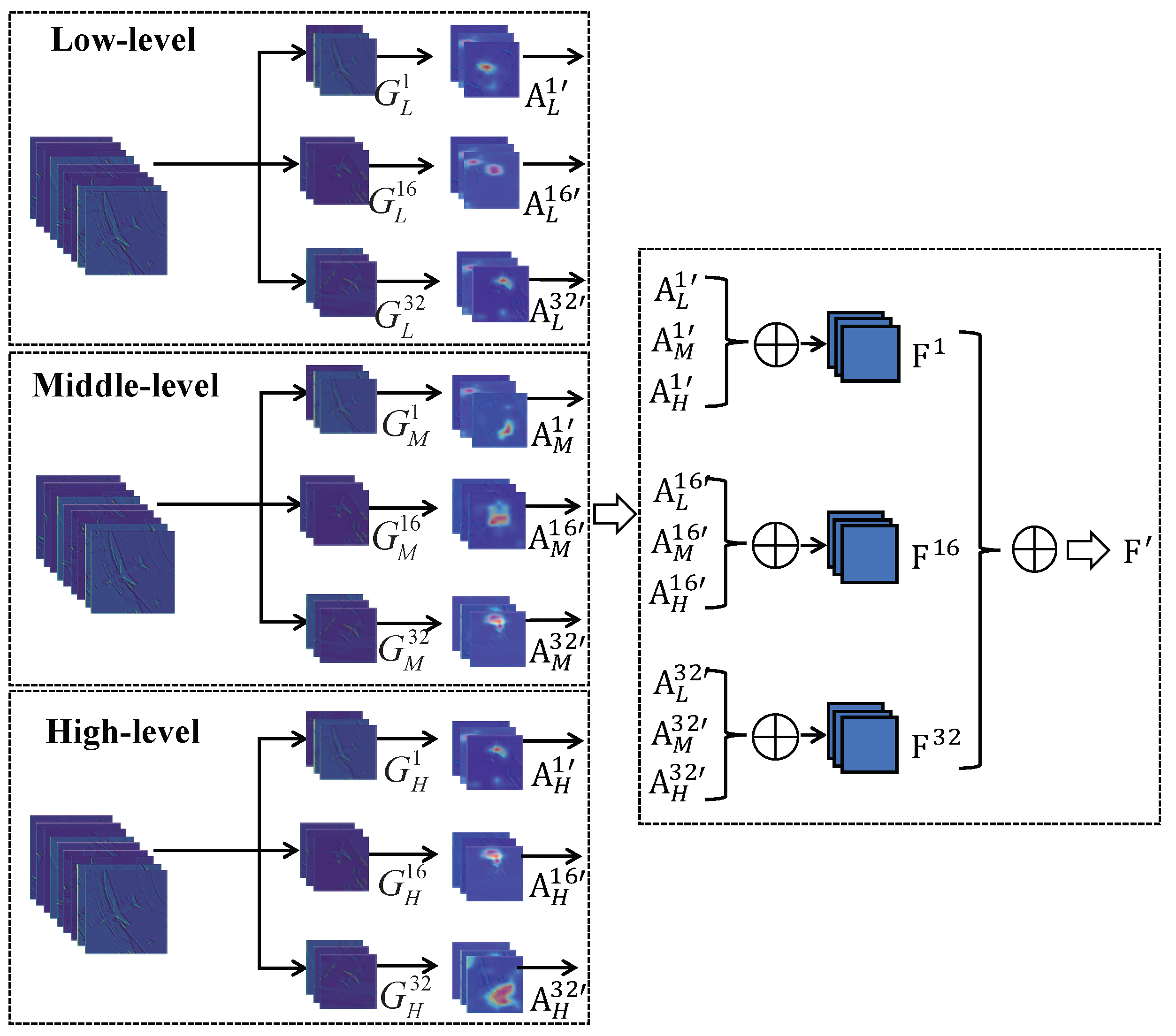
Specifically, the features of a certain level in one model are enhanced by a grouping step and an attention step. The grouping produces several subgroups along the channel dimension, and the attention is performed on each subgroup. This operation is conducted on each level, yielding the enhanced features of low-level, middle-level, and high-level, which are then fused by summation of the corresponding subgroup features. The fused features from the dual models are then added to generate the dual-model deep feature.
3.2.1. Grouping
The intuition of channel grouping is from the “Divide-and-Conquer” idea, which means that a set of subgroups can be solved more easily and efficiently than a whole group. Before fusing the multi-level features, each level feature is grouped into subgroups along the channel dimension to reduce the feature complexity. Specifically, grouping makes use of the new dimension, namely “cardinality” (noted as C), i.e., the feature channels are grouped into C subgroups, as shown in Figure 5. For example, considering the low-level features with 128 dimensions, when , the features are grouped into 32 subgroups, which are denoted as , where is the ith subgroup of the low-level features. The size of each subgroup is , where h is the height of the map and w is the width of the map. Likewise, the middle-level and high-level features are divided into subgroups, denoted as and , respectively.
3.2.2. Attention
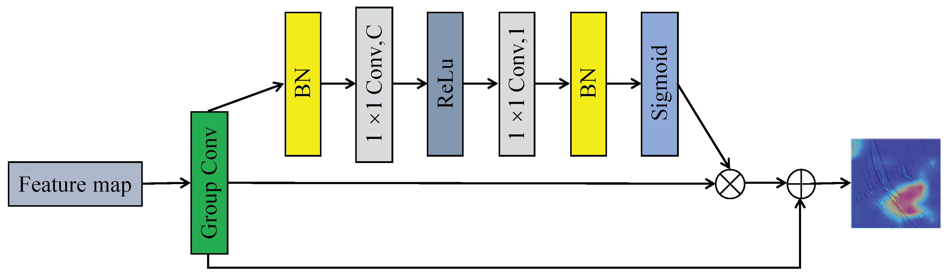
To pay attention to the key position of the scene, an explainable attention network [38] is introduced to our proposed strategy, as shown in Figure 6. The input is the subgroup feature map, denoted as F, the size of which is . The feature map is convoluted by a convolutional layer, generating C feature maps, followed by a convolution layer to generate a feature map. Then, the feature map is normalized by the sigmoid function, yielding the attention map A. The attention mechanism states that:
where is the output of this mechanism.
3.2.3. Fusion
After grouping and attention, the feature maps are added for fusion, according to the rule that the corresponding subgroups from three levels are added together. For instance, is the ith feature map of in the low-level, after the manipulations of grouping and attention. The feature maps of middle-level and high-level are denoted as and , respectively. Then, , , and are fused via summation, producing the fused sub-feature map of the ith subgroup. The fused feature map are generated by the summation of all the 32 sub-feature maps. The final fused feature map of the dual-model architecture is produced by concatenating the feature map F of each single model.
3.3. Classification with Metric Learning
The characteristics of remote sensing images bring the challenge of high intra-class diversity and inter-class similarity. This motivates us to develop a training objective that balances the intra-class and inter-class diversity during learning, which is also the target of metric learning. Intuitively, we propose a loss function, denoted as
where is the intra-class loss function for controlling the intra-class diversity, is the inter-class loss function for controlling the inter-class similarity, and is the balance parameter. Clearly, minimizing would result in the solution having low intra-class diversity and high inter-class diversity. To realize the above idea, we implement as the center loss [60]:
where represents the center of the th category, denotes the feature of the ith sample, and m denotes the batch size of samples of the th category. As seen, we constrain the samples of each category to be close to each other within the category, in which way the intra-class diversity could be minimized. To maximize the inter-class distance, is implemented as the focal loss [61]:
where denotes the feature of the ith sample, denotes the weights for classifying the jth category in the fully connected layer, is the bias term for the jth category, m denotes the batch size of samples of the th category, and n is the number of categories. The small inter-class distances between different classes are caused by hard examples. Regarding this, the focal loss can encourage the optimization to focus on the hard examples, i.e., the hard examples would contribute more on the gradients during back-propagation than the easy examples. Specifically, the value in the bracket reveals that how far the predicted label is from the ground-truth, i.e., the value being large when the prediction is incorrect (hard examples) and small otherwise (easy examples). According to the characteristics of the exponential function, when , the influence of easy examples will be suppressed more than the hard examples. Hence, this loss could address the issue of inter-class diversity, yielding improved performance.
4. Experiments
In this section, we conduct a series of experiments to validate the effectiveness of the proposed method.
4.1. Datasets
We employ four public datasets in experiments, which are detailed as follows.
- UC Merced Land-Use Dataset [39]: This dataset contains land-use scenes, which has been widely used in remote sensing scene classification. It consists of 21 scene categories and each category has 100 images with the size of . The ground sampling distance is 1 inch per pixel. This dataset is challenging because of high inter-class similarity, such as dense residential and sparse residential.
- WHU-RS19 Dataset [40]: The images of this dataset are collected from Google Earth, containing in total 950 images with the size of . The ground sampling distance is 0.5 m per pixel. There are 19 categories with great variation, such as commercial area, pond, football field, and desert, imposing great difficulty for classification.
- Aerial Image Dataset (AID) [42]: It is a large-scale dataset collected from Google Earth, containing 30 classes and 10000 images with the size of . The ground sampling distance ranges from 0.5 m per pixel to 8 m per pixel. The characteristic of this dataset is high intra-class diversity, since the same scene is captured under different imaging conditions and at different time, generating the images with the same content but different appearances.
- OPTIMAL-31 Dataset [43]: The dataset has 31 categories with each category collecting 60 images with the size of .
4.2. Evaluation Metrics
To assess the effectiveness of the proposed method, we use the widely used evaluation metrics including the overall accuracy (OA) and the confusion matrix (CM), which are described below.
- Overall accuracy (OA) is computed as the ratio of the correctly classified images to all images.
- Confusion matrix (CM) is constructed as the relation between the ground-truth label (in each row) and the predicted label (in each column). CM illustrates which category is easily confused with other categories in a visual way.
4.3. Experimental Settings
The proposed model is trained by stochastic gradient descent (SGD) with the momentum as 0.9, the initial learning rate as 0.001, and the weight decay penalty as 0.009. The learning rate is reduced by 10 times after 100 epochs. The training process of the proposed model is terminated after 150 epochs. All experiments are implemented with Python 3.6.5 and conducted under the environment of NVIDIA 2080Ti GPU.
Data augmentation is employed during training to improve the generalization performance, including rotation, flip, scaling, and translation. The dual model used in our work, i.e., ResNet and DenseNet, are initialized as the pre-trained models on ImageNet. The parameters of the layers that do not exist in the pre-trained models are initialized randomly.
4.4. Ablation Study
4.4.1. Discussion on Cardinality
The cardinality is an important parameter in our proposed grouping-attention-fusion strategy, which influences the feature flow in the architecture as well as the final classification accuracy. In Table 1, we present the performance of the model when using different values of cardinality. The experiments are conducted on the OPTIMAL-31 dataset, which contains more classes and fewer images among the other datasets and thus is more challenging. The effectiveness of the proposed method can be well examined under different parameter settings, which would comprehensively show the generalization ability. From Table 1, we see that as the value goes up, the accuracy increases, while the highest precision is obtained when cardinality is 32. Hence, in the following experiments, we setup cardinality as 32 to achieve the best performance.
4.4.2. Discussion on
In the format of the inter-class loss , the parameter is used to mine the hard samples during learning. Hence, a proper value of helps to enlarge the distances between different classes, or specifically, the hard samples of different classes. The effect of is investigated on the OPTIMAL-31 dataset and the results are illustrated in Table 2. As seen, when , is the original cross entropy loss. As increases, the accuracy is improved. In our experiments, we set to improve the performance in comparison.
4.4.3. Discussion on
Recall that the proposed loss function is consisted of and , which are balanced using the parameter . Different values of are investigated in Table 3, from which we see that the best performance is achieved when . Hence, we set in the following experiments.
4.5. Comparison with State-of-the-Arts
We compare the proposed method with the state-of-the-arts on the four datasets. To make a fair comparison, each experiment is repeated ten times, and the final performance is computed by averaging the results.
- UC Merced Land-Use Dataset:
In this dataset, we first setup two training settings including the training ratio of 80% and 50%, which means that the partition of training data is 80% and 50% of the whole dataset, respectively. The selected competitors and the results are shown in Table 4. The comparison indicates that the proposed model performs better than other methods in almost all cases. Similar methods to ours include ResNet-TP-50 [11] which adopts two-path ResNet as backbone, and Two-Stream Fusion [10] which extracts two-stream features from CNN models for fusion. The results show that both methods perform better than other single model-based methods under both training settings, demonstrating the superiority of the dual-model architecture over the single model architecture. The method of [12] introduces metric learning to the D-CNN model, but the accuracy is 1.22% lower than our method. This indicates that the proposed loss function is helpful to improve the accuracy.
To make comparison on a more challenging condition, we conduct a series of experiments by using the training ratio of 20% on this dataset. The results are presented in Table 5, which indicates that the proposed method achieves the best performance in this challenging case.
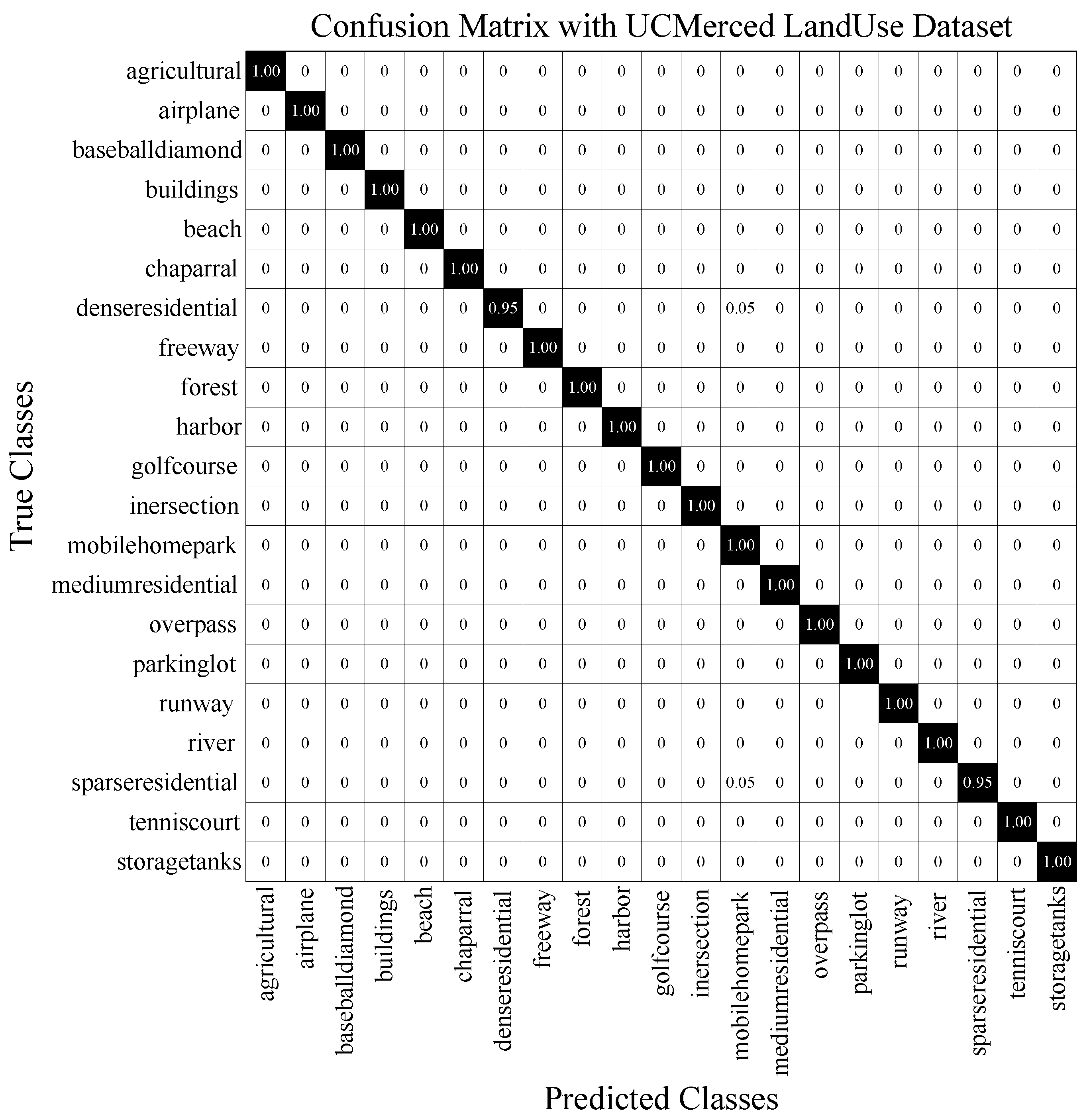
To inspect the class-wise performance of our method, confusion matrix (CM) is adopted, as shown in Figure 7. The error occurs when the dense residential is misclassified as the mobile home park and the sparse residential is misclassified as the mobile home park. This illustrates the confusing categories including mobile home park, dense residential, and sparse residential.
The above experimental results verify that the feature fusion mechanism and the metric learning-based loss could be beneficial to the scene classification.
- WHU-RS19 Dataset:
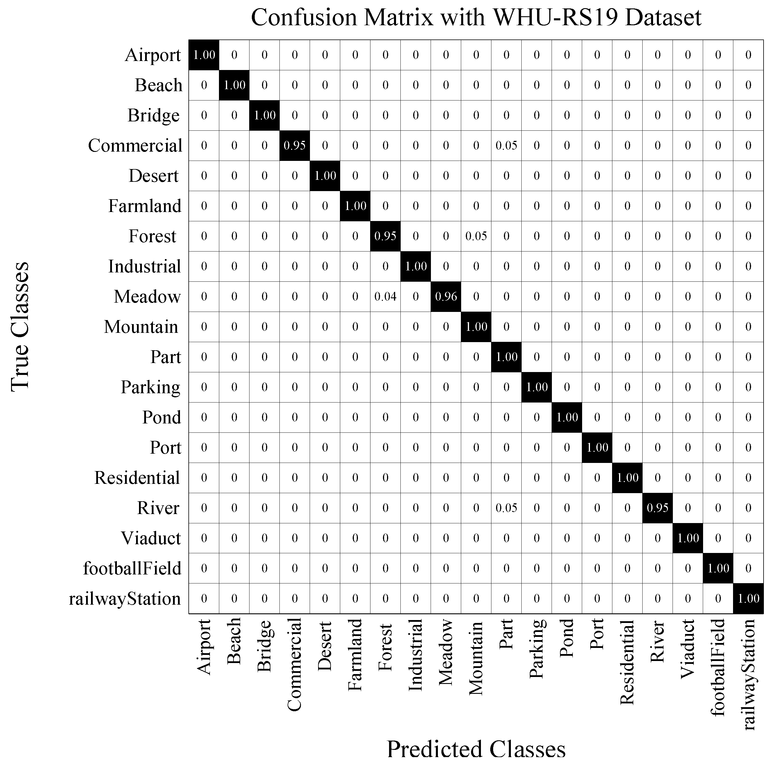
This dataset has the characteristics that the image quantity of each category is quite small, and the resolution of each image is high. We setup two training settings including the training ratio of 60% and 40%. The comparison results are illustrated in Table 6, which shows that the performance of our method exceeds that of most methods. The accuracy of ARCNet-VGG16 is 0.8% higher than that of our method at 60% training ratio, but our method surpasses at lower training ratio.
The CM of our method is shown in Figure 8, illustrating the confusing cases between forest and mountain, between meadow and forest, between river and park, and between commercial and part.
- Aerial Image Dataset (AID):
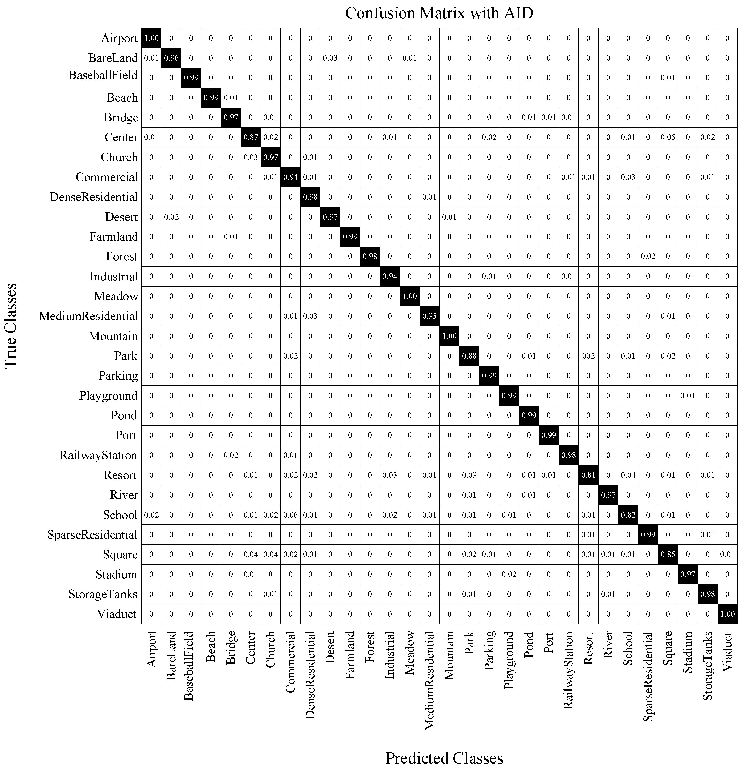
This dataset is a large one consisting of 10000 images. We setup two training settings including the training ratio of 50% and 20%. In both settings, our method performs better than all the competitors, as shown in Table 7. For example, our method has increased 3.02% over ARCNet-VGG16 [43] when the training ratio is 50%, and increased 5.3% when the training ratio is 20%. The results indicate that the proposed method perform well on large datasets, even when the available training data is limited. CM is shown in Figure 9, from which we observe very small possibility between confusing categories.
- OPTIMAL-31 Dataset:
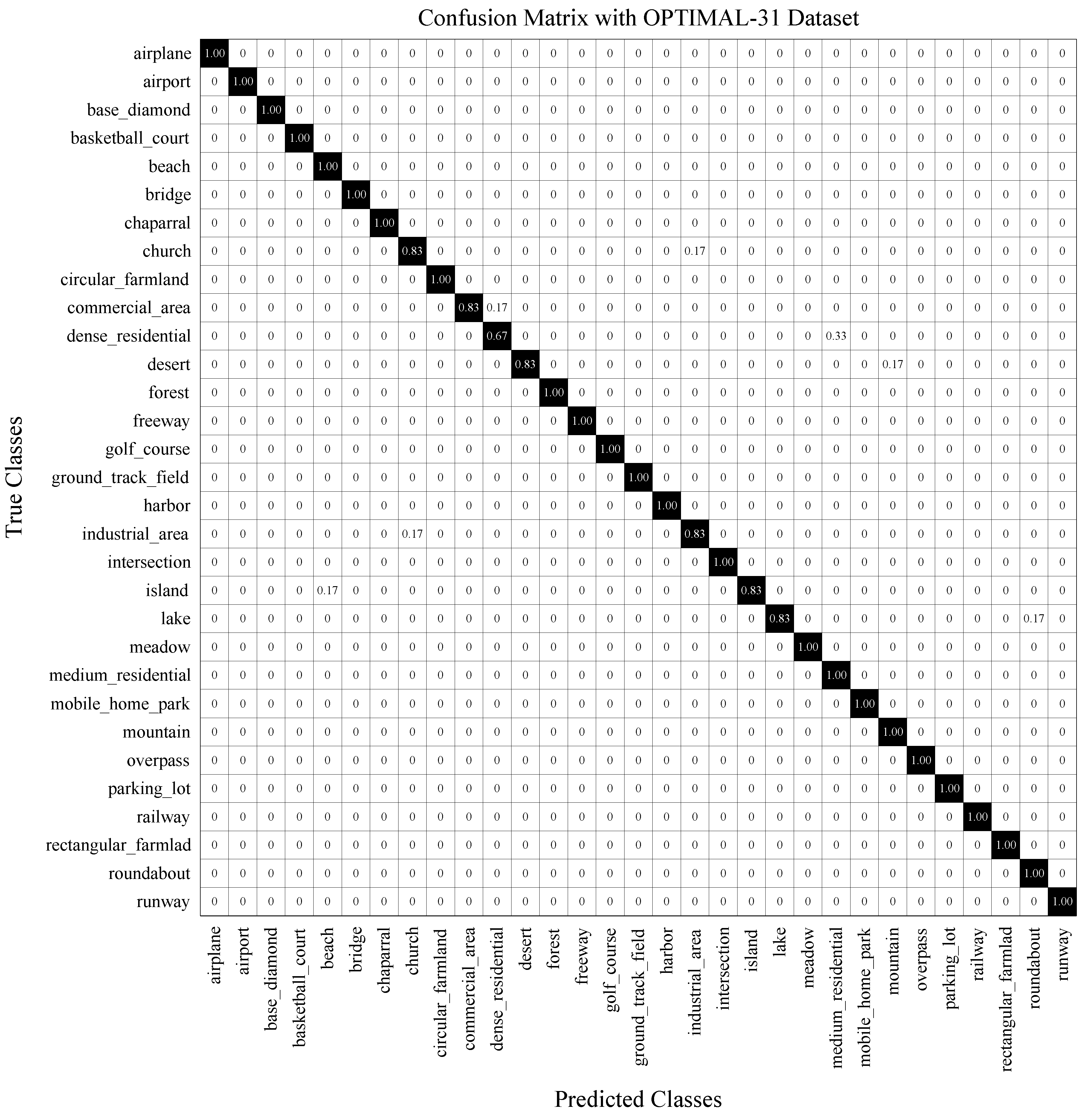
This dataset is recently published, and the performance of several states of the art are available. The results are presented in Table 8, which shows that our method outperforms the state-of-art methods in all cases. Regarding the CM shown in Figure 10, we observe very limited cases of confusing categories.
4.6. Discussions
In this section, we give a brief discussion on why the proposed method could improve the performance compared with the competitors. The proposed method is closely related to [10] which introduces a two-stream architecture that extracts features from both an original remote sensing image and a pre-processed image via saliency detection, yielding very competitive performance in comparison (see Table 4, Table 6 and Table 7). It is demonstrated that the fusion of multi-stream information is effective in scene classification. We refer the two-stream idea and propose a dual-CNN architecture which, however, differs in that the features of multiple hierarchical levels (i.e., low-level, medium-level, and high-level) of two CNNs are exploited. In this way, the extracted features are complementary with each other and hence, the fusion produces a more comprehensive feature representation. This is especially beneficial for multi-scale object analyses. Moreover, we elaborate the fusion process by dividing the channels into small groups. The attention operation in each small group could excavate fine-grained saliency information, which is empirically shown effective.
We also compare with a related method DDRL-AM [65] (see Table 4) which enhances the feature representation by integrating the attention map with the center loss-based discriminative learning. By contrast, we improve the center loss by adding a factor in the measurement of inter-class loss, such that the learning process could suppress the losses of easy samples and focus on the hard samples. This is similar to the focal loss used in object detection [61]. The comparison validates the superiority of the proposed method over DDRL-AM [65].
The recently published second-order feature-based methods could produce pleasing performance on fine-grained classification tasks including remote sensing scene classification, e.g., [57]. Typically, the multilayer stacked covariance pooling (MSCP) method [57] exploits the covariance pooling operation among the multilayer feature maps of a CNN model, which is indeed a kind of feature fusion scheme. Such a second-order feature representation reveals the fine distortions of the objects in images. Although this method produces comparable results to the state-of-the-arts in Table 4 and Table 7, it is a post-processing method and does not benefit from the end-to-end learning. Instead, the proposed method yields a fusion process which is optimized in conjunction with the whole model learning and hence, produces improved performance in most cases.
5. Conclusions
Remote sensing scene classification is a challenging task that brings the difficulties of complex background, various imaging conditions, multi-scale objects, and similar appearances. Targeting on these issues, on this work, we propose a novel dual-model architecture with deep feature fusion. The dual-model architecture could compensate the deficiency of a single model, especially by improving the representation capacity of the model. A grouping-attention-fusion strategy is developed to enhance the discrimination ability of the extracted features and fuse the multi-scale information coming from two models. The resultant feature representation has a more comprehensive information than the feature of a single model. To encourage small intra-class diversity and large inter-class distance, we propose a novel loss function to reduce the confusion between different classes, which yields better performance in scene classification. Extensive experiments are conducted on four challenging datasets. The results demonstrate that the dual-model architecture is more effective than one single model, and the proposed feature fusion strategy provides more elaborative features to improve classification accuracy. Moreover, the metric learning-based loss function is well-suited for the scene-classification problem of high intra-class diversity and inter-class similarity. The comparison verifies the superiority of the proposed model over the state-of-the-arts.
Author Contributions
Conceptualization, J.S. and R.W.; methodology, J.S., T.Z., and R.W.; software, T.Z. and Y.W.; validation, T.Z. and Y.W.; formal analysis, J.S., R.W., and Q.W.; investigation, J.S. and M.Q.; resources, R.W. and Q.W.; data curation, M.Q.; writing—original draft preparation, J.S.; writing—review and editing, R.W.; visualization, T.Z.; supervision, J.S., R.W., and Q.W.; project administration, J.S. and R.W.; funding acquisition, J.S. All authors have read and agreed to the published version of the manuscript.
Funding
This research was funded by National Natural Science Foundation of China grant numbers 61603233 and 51909206, and the Project for “1000 Talents Plan for Young Talents of Yunnan Province”.
Data Availability Statement
The data used to support the findings of this study are available from the corresponding author upon request.
Acknowledgments
The authors wish to acknowledge the Key Laboratory of Underwater Intelligent Equipment of Henan Province for offering the strong support throughout the experiments.
Conflicts of Interest
The authors declare no conflict of interest.
Abbreviations
The following abbreviations are used in this manuscript:
| CNN | convolutional neural networks |
| UCM | UC Merced Land-Use Dataset |
| AID | Aerial Image Dataset |
| GAP | grouping-attention-fusion |
| OA | overall accuracy |
| CM | confusion matrix |
| SGD | stochastic gradient descent |
References
- Cheng, G.; Han, J.; Guo, L.; Liu, Z.; Bu, S.; Ren, J. Effective and efficient midlevel visual elements-oriented land-use classification using VHR remote sensing images. IEEE Trans. Geosci. Remote Sens. 2015, 53, 4238–4249. [Google Scholar] [CrossRef] [Green Version]
- Hu, F.; Yang, W.; Chen, J.; Sun, H. Tile-level annotation of satellite images using multi-level max-margin discriminative random field. Remote Sens. 2013, 5, 2275–2291. [Google Scholar] [CrossRef] [Green Version]
- Hu, F.; Xia, G.S.; Hu, J.; Zhang, L. Transferring deep convolutional neural networks for the scene classification of high-resolution remote sensing imagery. Remote Sens. 2015, 7, 14680–14707. [Google Scholar] [CrossRef] [Green Version]
- Cheng, G.; Li, Z.; Yao, X.; Guo, L.; Wei, Z. Remote sensing image scene classification using bag of convolutional features. IEEE Geosci. Remote Sens. Lett. 2017, 14, 1735–1739. [Google Scholar] [CrossRef]
- Xu, K.; Huang, H.; Li, Y.; Shi, G. Multilayer Feature Fusion Network for Scene Classification in Remote Sensing. IEEE Geosci. Remote Sens. Lett. 2020, 17, 1894–1898. [Google Scholar] [CrossRef]
- Krizhevsky, A.; Sutskever, I.; Hinton, G.E. Imagenet classification with deep convolutional neural networks. Commun. ACM 2017, 60, 84–90. [Google Scholar] [CrossRef]
- Simonyan, K.; Zisserman, A. Very deep convolutional networks for large-scale image recognition. arXiv 2014, arXiv:1409.1556. [Google Scholar]
- He, K.; Zhang, X.; Ren, S.; Sun, J. Deep residual learning for image recognition. In Proceedings of the IEEE Conference on Computer Vision and Pattern Recognition, Las Vegas, NV, USA, 27–30 June 2016; pp. 770–778. [Google Scholar]
- Huang, G.; Liu, Z.; Van Der Maaten, L.; Weinberger, K.Q. Densely connected convolutional networks. In Proceedings of the IEEE Conference on Computer Vision and Pattern Recognition, Honolulu, HI, USA, 21–26 July 2017; pp. 4700–4708. [Google Scholar]
- Yu, Y.; Liu, F. A two-stream deep fusion framework for high-resolution aerial scene classification. Comput. Intell. Neurosci. 2018, 2018, 8639367. [Google Scholar] [CrossRef] [Green Version]
- Zhou, Z.; Zheng, Y.; Ye, H.; Pu, J.; Sun, G. Satellite image scene classification via ConvNet with context aggregation. In Pacific Rim Conference on Multimedia; Springer: Berlin/Heidelberg, Germany, 2018; pp. 329–339. [Google Scholar]
- Cheng, G.; Yang, C.; Yao, X.; Guo, L.; Han, J. When deep learning meets metric learning: Remote sensing image scene classification via learning discriminative CNNs. IEEE Trans. Geosci. Remote Sens. 2018, 56, 2811–2821. [Google Scholar] [CrossRef]
- Bian, X.; Chen, C.; Tian, L.; Du, Q. Fusing local and global features for high-resolution scene classification. IEEE J. Sel. Top. Appl. Earth Obs. Remote Sens. 2017, 10, 2889–2901. [Google Scholar] [CrossRef]
- Huang, L.; Chen, C.; Li, W.; Du, Q. Remote sensing image scene classification using multi-scale completed local binary patterns and fisher vectors. Remote Sens. 2016, 8, 483. [Google Scholar] [CrossRef] [Green Version]
- Chen, C.; Zhang, B.; Su, H.; Li, W.; Wang, L. Land-use scene classification using multi-scale completed local binary patterns. Signal Image Video Process. 2016, 10, 745–752. [Google Scholar] [CrossRef]
- Cheng, G.; Zhou, P.; Han, J.; Guo, L.; Han, J. Auto-encoder-based shared mid-level visual dictionary learning for scene classification using very high resolution remote sensing images. IET Comput. Vis. 2015, 9, 639–647. [Google Scholar] [CrossRef]
- Cheng, G.; Han, J.; Zhou, P.; Guo, L. Multi-class geospatial object detection and geographic image classification based on collection of part detectors. ISPRS J. Photogramm. Remote Sens. 2014, 98, 119–132. [Google Scholar] [CrossRef]
- Cheng, G.; Han, J.; Guo, L.; Liu, T. Learning coarse-to-fine sparselets for efficient object detection and scene classification. In Proceedings of the IEEE Conference on Computer Vision and Pattern Recognition, Boston, MA, USA, 7–12 June 2015; pp. 1173–1181. [Google Scholar]
- Zou, J.; Li, W.; Chen, C.; Du, Q. Scene classification using local and global features with collaborative representation fusion. Inf. Sci. 2016, 348, 209–226. [Google Scholar] [CrossRef]
- Lu, X.; Li, X.; Mou, L. Semi-supervised multitask learning for scene recognition. IEEE Trans. Cybern. 2014, 45, 1967–1976. [Google Scholar]
- Chaib, S.; Liu, H.; Gu, Y.; Yao, H. Deep feature fusion for VHR remote sensing scene classification. IEEE Trans. Geosci. Remote Sens. 2017, 55, 4775–4784. [Google Scholar] [CrossRef]
- Othman, E.; Bazi, Y.; Melgani, F.; Alhichri, H.; Alajlan, N.; Zuair, M. Domain adaptation network for cross-scene classification. IEEE Trans. Geosci. Remote Sens. 2017, 55, 4441–4456. [Google Scholar] [CrossRef]
- Zhang, F.; Du, B.; Zhang, L. Scene classification via a gradient boosting random convolutional network framework. IEEE Trans. Geosci. Remote Sens. 2015, 54, 1793–1802. [Google Scholar] [CrossRef]
- Cheng, G.; Zhou, P.; Han, J. Learning rotation-invariant convolutional neural networks for object detection in VHR optical remote sensing images. IEEE Trans. Geosci. Remote Sens. 2016, 54, 7405–7415. [Google Scholar] [CrossRef]
- Li, E.; Xia, J.; Du, P.; Lin, C.; Samat, A. Integrating multilayer features of convolutional neural networks for remote sensing scene classification. IEEE Trans. Geosci. Remote Sens. 2017, 55, 5653–5665. [Google Scholar] [CrossRef]
- Wang, G.; Fan, B.; Xiang, S.; Pan, C. Aggregating rich hierarchical features for scene classification in remote sensing imagery. IEEE J. Sel. Top. Appl. Earth Obs. Remote Sens. 2017, 10, 4104–4115. [Google Scholar] [CrossRef]
- Yao, X.; Han, J.; Cheng, G.; Qian, X.; Guo, L. Semantic annotation of high-resolution satellite images via weakly supervised learning. IEEE Trans. Geosci. Remote Sens. 2016, 54, 3660–3671. [Google Scholar] [CrossRef]
- Zhao, W.; Du, S. Scene classification using multi-scale deeply described visual words. Int. J. Remote Sens. 2016, 37, 4119–4131. [Google Scholar] [CrossRef]
- Luus, F.P.; Salmon, B.P.; Van den Bergh, F.; Maharaj, B.T.J. Multiview deep learning for land-use classification. IEEE Geosci. Remote Sens. Lett. 2015, 12, 2448–2452. [Google Scholar] [CrossRef] [Green Version]
- Marmanis, D.; Datcu, M.; Esch, T.; Stilla, U. Deep learning earth observation classification using ImageNet pretrained networks. IEEE Geosci. Remote Sens. Lett. 2015, 13, 105–109. [Google Scholar] [CrossRef] [Green Version]
- Nogueira, K.; Penatti, O.A.; Dos Santos, J.A. Towards better exploiting convolutional neural networks for remote sensing scene classification. Pattern Recognit. 2017, 61, 539–556. [Google Scholar] [CrossRef] [Green Version]
- Zhang, L.; Zhang, L.; Du, B. Deep learning for remote sensing data: A technical tutorial on the state of the art. IEEE Geosci. Remote Sens. Mag. 2016, 4, 22–40. [Google Scholar] [CrossRef]
- Lowe, D.G. Distinctive image features from scale-invariant keypoints. Int. J. Comput. Vis. 2004, 60, 91–110. [Google Scholar] [CrossRef]
- Risojević, V.; Babić, Z. Fusion of global and local descriptors for remote sensing image classification. IEEE Geosci. Remote Sens. Lett. 2012, 10, 836–840. [Google Scholar] [CrossRef]
- Zhu, Q.; Zhong, Y.; Zhao, B.; Xia, G.S.; Zhang, L. Bag-of-visual-words scene classifier with local and global features for high spatial resolution remote sensing imagery. IEEE Geosci. Remote Sens. Lett. 2016, 13, 747–751. [Google Scholar] [CrossRef]
- Wu, Z.; Shi, L.; Li, J.; Wang, Q.; Sun, L.; Wei, Z.; Plaza, J.; Plaza, A. GPU parallel implementation of spatially adaptive hyperspectral image classification. IEEE J. Sel. Top. Appl. Earth Obs. Remote Sens. 2017, 11, 1131–1143. [Google Scholar] [CrossRef]
- Wu, Z.; Li, Y.; Plaza, A.; Li, J.; Xiao, F.; Wei, Z. Parallel and distributed dimensionality reduction of hyperspectral data on cloud computing architectures. IEEE J. Sel. Top. Appl. Earth Obs. Remote Sens. 2016, 9, 2270–2278. [Google Scholar] [CrossRef]
- Fukui, H.; Hirakawa, T.; Yamashita, T.; Fujiyoshi, H. Attention branch network: Learning of attention mechanism for visual explanation. In Proceedings of the IEEE Conference on Computer Vision and Pattern Recognition, Long Beach, CA, USA, 15–20 June 2019; pp. 10705–10714. [Google Scholar]
- Yang, Y.; Newsam, S. Bag-of-visual-words and spatial extensions for land-use classification. In Proceedings of the 18th SIGSPATIAL International Conference on Advances in Geographic Information Systems, San Jose, CA, USA, 2–5 November 2010; pp. 270–279. [Google Scholar]
- Sheng, G.; Yang, W.; Xu, T.; Sun, H. High-resolution satellite scene classification using a sparse coding based multiple feature combination. Int. J. Remote Sens. 2012, 33, 2395–2412. [Google Scholar] [CrossRef]
- Kalajdjieski, J.; Zdravevski, E.; Corizzo, R.; Lameski, P.; Kalajdziski, S.; Pires, I.M.; Garcia, N.M.; Trajkovik, V. Air Pollution Prediction with Multi-Modal Data and Deep Neural Networks. Remote Sens. 2020, 12, 4142. [Google Scholar] [CrossRef]
- Xia, G.S.; Hu, J.; Hu, F.; Shi, B.; Bai, X.; Zhong, Y.; Zhang, L.; Lu, X. AID: A benchmark data set for performance evaluation of aerial scene classification. IEEE Trans. Geosci. Remote Sens. 2017, 55, 3965–3981. [Google Scholar] [CrossRef] [Green Version]
- Wang, Q.; Liu, S.; Chanussot, J.; Li, X. Scene classification with recurrent attention of VHR remote sensing images. IEEE Trans. Geosci. Remote Sens. 2018, 57, 1155–1167. [Google Scholar] [CrossRef]
- Othman, E.; Bazi, Y.; Alajlan, N.; Alhichri, H.; Melgani, F. Using convolutional features and a sparse autoencoder for land-use scene classification. Int. J. Remote Sens. 2016, 37, 2149–2167. [Google Scholar] [CrossRef]
- Scott, G.J.; England, M.R.; Starms, W.A.; Marcum, R.A.; Davis, C.H. Training deep convolutional neural networks for land–cover classification of high-resolution imagery. IEEE Geosci. Remote Sens. Lett. 2017, 14, 549–553. [Google Scholar] [CrossRef]
- Yu, Y.; Liu, F. Aerial scene classification via multilevel fusion based on deep convolutional neural networks. IEEE Geosci. Remote Sens. Lett. 2018, 15, 287–291. [Google Scholar] [CrossRef]
- Boualleg, Y.; Farah, M.; Farah, I.R. Remote sensing scene classification using convolutional features and deep forest classifier. IEEE Geosci. Remote Sens. Lett. 2019, 16, 1944–1948. [Google Scholar] [CrossRef]
- Guo, Y.; Ji, J.; Lu, X.; Huo, H.; Fang, T.; Li, D. Global-local attention network for aerial scene classification. IEEE Access 2019, 7, 67200–67212. [Google Scholar] [CrossRef]
- Wang, F.; Jiang, M.; Qian, C.; Yang, S.; Li, C.; Zhang, H.; Wang, X.; Tang, X. Residual attention network for image classification. In Proceedings of the IEEE Conference on Computer Vision and Pattern Recognition, Honolulu, HI, USA, 21–26 July 2017; pp. 3156–3164. [Google Scholar]
- Xiong, W.; Lv, Y.; Cui, Y.; Zhang, X.; Gu, X. A discriminative feature learning approach for remote sensing image retrieval. Remote Sens. 2019, 11, 281. [Google Scholar] [CrossRef] [Green Version]
- Zhao, Z.; Luo, Z.; Li, J.; Chen, C.; Piao, Y. When Self-Supervised Learning Meets Scene Classification: Remote Sensing Scene Classification Based on a Multitask Learning Framework. Remote Sens. 2020, 12, 3276. [Google Scholar] [CrossRef]
- Castelluccio, M.; Poggi, G.; Sansone, C.; Verdoliva, L. Land use classification in remote sensing images by convolutional neural networks. arXiv 2015, arXiv:1508.00092. [Google Scholar]
- Shao, W.; Yang, W.; Xia, G.S.; Liu, G. A hierarchical scheme of multiple feature fusion for high-resolution satellite scene categorization. In Proceedings of the International Conference on Computer Vision Systems, St. Petersburg, Russia, 16–18 July 2013; Springer: Berlin/Heidelberg, Germany, 2013; pp. 324–333. [Google Scholar]
- Liu, Y.; Liu, Y.; Ding, L. Scene classification based on two-stage deep feature fusion. IEEE Geosci. Remote Sens. Lett. 2017, 15, 183–186. [Google Scholar] [CrossRef]
- Yu, Y.; Liu, F. Dense connectivity based two-stream deep feature fusion framework for aerial scene classification. Remote Sens. 2018, 10, 1158. [Google Scholar] [CrossRef] [Green Version]
- Petrovska, B.; Zdravevski, E.; Lameski, P.; Corizzo, R.; Štajduhar, I.; Lerga, J. Deep learning for feature extraction in remote sensing: A case-study of aerial scene classification. Sensors 2020, 20, 3906. [Google Scholar] [CrossRef]
- He, N.; Fang, L.; Li, S.; Plaza, A.; Plaza, J. Remote Sensing Scene Classification Using Multilayer Stacked Covariance Pooling. IEEE Trans. Geosci. Remote Sens. 2018, 56, 6899–6919. [Google Scholar] [CrossRef]
- Akodad, S.; Bombrun, L.; Xia, J.; Berthoumieu, Y.; Germain, C. Ensemble Learning Approaches Based on Covariance Pooling of CNN Features for High Resolution Remote Sensing Scene Classification. Remote Sens. 2020, 12, 3292. [Google Scholar] [CrossRef]
- Zhang, Y.; Guo, L.; Wang, Z.; Yu, Y.; Liu, X.; Xu, F. Intelligent Ship Detection in Remote Sensing Images Based on Multi-Layer Convolutional Feature Fusion. Remote Sens. 2020, 12, 3316. [Google Scholar] [CrossRef]
- Wen, Y.; Zhang, K.; Li, Z.; Qiao, Y. A discriminative feature learning approach for deep face recognition. In Proceedings of the European Conference on Computer Vision, Amsterdam, The Netherlands, 8–16 October 2016; pp. 499–515. [Google Scholar]
- Lin, T.Y.; Goyal, P.; Girshick, R.; He, K.; Dollár, P. Focal loss for dense object detection. In Proceedings of the IEEE International Conference on Computer Vision, Venice, Italy, 22–29 October 2017; pp. 2980–2988. [Google Scholar]
- Chen, S.; Tian, Y. Pyramid of spatial relatons for scene-level land use classification. IEEE Trans. Geosci. Remote Sens. 2014, 53, 1947–1957. [Google Scholar] [CrossRef]
- Zhang, F.; Du, B.; Zhang, L. Saliency-guided unsupervised feature learning for scene classification. IEEE Trans. Geosci. Remote Sens. 2014, 53, 2175–2184. [Google Scholar] [CrossRef]
- Cheriyadat, A.M. Unsupervised feature learning for aerial scene classification. IEEE Trans. Geosci. Remote Sens. 2013, 52, 439–451. [Google Scholar] [CrossRef]
- Li, J.; Lin, D.; Wang, Y.; Xu, G.; Zhang, Y.; Ding, C.; Zhou, Y. Deep Discriminative Representation Learning with Attention Map for Scene Classification. Remote Sens. 2020, 12, 1366. [Google Scholar] [CrossRef]
Figure 1.
The scene of a remote sensing image contains many kinds of objects.

Figure 2.
Two remote sensing scene images labeled as “plane”. (a) The image contains “large planes”. (b) The image contains many “small planes”.
Figure 2.
Two remote sensing scene images labeled as “plane”. (a) The image contains “large planes”. (b) The image contains many “small planes”.

Figure 3.
The examples of high intra-class diversity and inter-class similarity. The images in (a1,a2) have similar appearances which, however, are labeled as different classes, i.e., “school” v.s. “park”. The images in (b1,b2) have the same label of “center” but have variant appearances.
Figure 3.
The examples of high intra-class diversity and inter-class similarity. The images in (a1,a2) have similar appearances which, however, are labeled as different classes, i.e., “school” v.s. “park”. The images in (b1,b2) have the same label of “center” but have variant appearances.

Figure 4.
The overall architecture of our proposed method.

Figure 5.
The grouping-attention-fusion strategy.

Figure 6.
The feature attention module.

Figure 7.
CM on UCM Land-Use dataset under the training ratio of 80%.

Figure 8.
CM on WHU RS19 dataset under the training ratio of 60%.

Figure 9.
CM on AID under the training ratio of 50%.

Figure 10.
CM on OPTIMAL-31 under the training ratio of 80%.


Table 1.
Investigation of cardinality.
| Cardinality | OA(%) |
|---|---|
| 1 | 94.62 |
| 4 | 94.09 |
| 8 | 94.62 |
| 16 | 95.70 |
| 32 | 96.24 |
| 64 | 93.28 |
Table 2.
Investigation of .
| OA (%) | |
|---|---|
| = 0 | 94.09 |
| = 1 | 95.16 |
| = 2 | 95.70 |
Table 3.
Investigation of .
| OA (%) | |
|---|---|
| 0.0001 | 93.28 |
| 0.0005 | 95.16 |
| 0.005 | 94.62 |
| 0.01 | 94.09 |
| 0.05 | 93.55 |
Table 4.
The OA(%) of different methods on UC Merced Land-Use Dataset. The “w.r.t. baseline” column lists the improvements of the corresponding methods with respect to the baseline GoogLeNet.
Table 4.
The OA(%) of different methods on UC Merced Land-Use Dataset. The “w.r.t. baseline” column lists the improvements of the corresponding methods with respect to the baseline GoogLeNet.
| Methods | 80% Images for Training | w.r.t. Baseline (80%) | 50% Images for Training | w.r.t. Baseline (50%) |
|---|---|---|---|---|
| ARCNet-VGG16 [43] | 99.12 ± 0.40 | +4.81 | 96.81 ± 0.14 | +4.11 |
| Combing Scenarios I and II [3] | 98.49 | +4.18 | ||
| D-CNN with VGGNet-16 [12] | 98.93 ± 0.10 | +4.62 | ||
| Fusion by Addition [21] | 97.42 ± 1.79 | +3.11 | ||
| ResNet-TP-50 [11] | 98.56 ± 0.53 | +4.25 | 97.68 ± 0.26 | +4.98 |
| Two-Stream Fusion [10] | 98.02 ± 1.03 | +3.71 | 96.97 ± 0.75 | +4.27 |
| CNN-NN [44] | 97.19 | +2.88 | ||
| Fine-tuning GoogLeNet [52] | 97.10 | +2.79 | ||
| GoogLeNet [42] | 94.31 ± 0.89 | 0 | 92.70 ± 0.60 | 0 |
| CaffeNet [42] | 95.02 ± 0.81 | +0.71 | 93.98 ± 0.67 | +1.28 |
| Overfeat [31] | 90.91 ± 1.19 | −3.4 | ||
| VGG-VD-16 [42] | 95.21 ± 1.20 | +0.9 | 94.14 ± 0.69 | +1.44 |
| MS-CLBP+FV [14] | 93.00 ± 1.20 | −1.31 | 88.76 ± 0.76 | −3.94 |
| Gradient Boosting Random CNNS [23] | 94.53 | +0.22 | ||
| SalM3LBPCLM [13] | 95.75 ± 0.80 | +1.44 | 94.21 ± 0.75 | +1.51 |
| Partlets-based [1] | 91.33 ± 1.11 | −2.98 | ||
| Multifeature Concatenation [53] | 92.38 ± 0.62 | −1.93 | ||
| Pyramid of Spatial Relations [54] | 89.10 | −5.21 | ||
| Saliency-guided Feature Learning [62] | 82.72 ± 1.18 | −11.59 | ||
| Unsupervised Feature Learning [63] | 82.67 ± 1.23 | −11.64 | ||
| BoVW [64] | 76.81 | −17.5 | ||
| BiMobileNet (MobileNetv2) [52] | 99.03 ± 0.28 | +4.72 | 98.45 ± 0.27 | +5.75 |
| DDRL-AM [65] | 99.05 ± 0.08 | +4.74 | ||
| AlexNet+MSCP [57] | 97.29 ± 0.63 | +2.98 | ||
| AlexNet+MSCP+MRA [57] | 97.32 ± 0.52 | +3.01 | ||
| VGG-VD16+MSCP [57] | 98.36 ± 0.58 | +4.05 | ||
| VGG-VD16+MSCP+MRA [57] | 98.40 ± 0.34 | +4.09 | ||
| Ours | 99.52 ± 0.23 | +5.21 | 98.19 ± 0.39 | +5.49 |
Table 5.
A challenging comparison on UC Merced Land-Use Dataset. The “w.r.t. baseline” column lists the improvements of the corresponding methods with respect to the baseline GoogLeNet.
Table 5.
A challenging comparison on UC Merced Land-Use Dataset. The “w.r.t. baseline” column lists the improvements of the corresponding methods with respect to the baseline GoogLeNet.
| Methods | 20% Images for Training | w.r.t. Baseline |
|---|---|---|
| AlexNet [43] | 88.35 ± 0.85 | −0.84 |
| CaffeNet [43] | 90.48 ± 0.78 | +1.29 |
| GoogLeNet [43] | 89.19 ± 1.19 | 0 |
| VGG-16 [42] | 90.70 ± 0.68 | +1.51 |
| VGG-19 [43] | 89.76 ± 0.69 | +0.57 |
| ResNet-50 [43] | 91.93 ± 0.61 | +2.74 |
| ResNet-152 [43] | 92.47 ± 0.43 | +3.28 |
| Ours | 95.60 ± 0.39 | +6.41 |
Table 6.
The OA(%) of different methods on WHU-RS19 Dataset. The “w.r.t. baseline” column lists the improvements of the corresponding methods with respect to the baseline GoogLeNet.
Table 6.
The OA(%) of different methods on WHU-RS19 Dataset. The “w.r.t. baseline” column lists the improvements of the corresponding methods with respect to the baseline GoogLeNet.
| Methods | 60% Images for Training | w.r.t. Baseline (60%) | 40% Images for Training | w.r.t. Baseline (40%) |
|---|---|---|---|---|
| ARCNet-VGG16 [43] | 99.75 ± 0.25 | +5.04 | 97.50 ± 0.49 | +4.38 |
| Combing Scenarios I and II [3] | 98.89 | +4.18 | ||
| Fusion by Addition [21] | 98.65 ± 0.43 | +3.94 | ||
| Two-Stream Fusion [10] | 98.92 ± 0.52 | +4.21 | 98.23 ± 0.56 | +5.11 |
| VGG-VD-16 [42] | 96.05 ± 0.91 | +1.34 | 95.44 ± 0.60 | +2.32 |
| CaffeNet [42] | 96.24 ± 0.56 | +1.53 | 95.11 ± 1.20 | +1.99 |
| GoogLeNet [42] | 94.71 ± 1.33 | 0 | 93.12 ± 0.82 | 0 |
| SalM3LBPCLM [13] | 96.38 ± 0.82 | +1.67 | 95.35 ± 0.76 | +2.23 |
| Multifeature Concatenation [53] | 94.53 ± 1.01 | −0.18 | ||
| MS-CLBP+FV [14] | 94.32 ± 1.02 | −0.39 | ||
| MS-CLBP+BoVW [14] | 89.29 ± 1.30 | −5.42 | ||
| Bag of SIFT [62] | 85.52 ± 1.23 | −9.19 | ||
| Ours | 98.96 ± 0.78 | +4.25 | 97.98 ± 0.84 | +4.86 |
Table 7.
The OA(%) of different methods on Aerial Image Dataset(AID). The “w.r.t. baseline” column lists the improvements of the corresponding methods with respect to the baseline GoogLeNet.
Table 7.
The OA(%) of different methods on Aerial Image Dataset(AID). The “w.r.t. baseline” column lists the improvements of the corresponding methods with respect to the baseline GoogLeNet.
| Methods | 50% Images for Training | w.r.t. Baseline (50%) | 20% Images for Training | w.r.t. Baseline (20%) |
|---|---|---|---|---|
| ARCNet-VGG16 [43] | 93.10 ± 0.55 | +6.71 | 88.75 ± 0.40 | +5.31 |
| Fusion by Addition [21] | 91.87 ± 0.36 | +5.48 | ||
| Two-Stream Fusion [10] | 94.58 ± 0.25 | +8.19 | 92.32 ± 0.41 | +8.88 |
| D-CNN with AlexNet [12] | 94.47 ± 0.12 | +8.08 | 85.62 ± 0.10 | +2.18 |
| VGG-VD-16 [42] | 89.64 ± 0.36 | +3.25 | 86.59 ± 0.29 | +3.15 |
| CaffeNet [42] | 89.53 ± 0.31 | +3.14 | 86.86 ± 0.47 | +3.42 |
| GoogLeNet [42] | 86.39 ± 0.55 | 0 | 83.44 ± 0.40 | 0 |
| AlexNet+MSCP [57] | 92.36 ± 0.21 | +8.92 | 88.99 ± 0.38 | +2.6 |
| AlexNet+MSCP+MRA [57] | 94.11 ± 0.15 | +10.67 | 90.65 ± 0.19 | +4.26 |
| VGG-VD16+MSCP [57] | 94.42 ± 0.17 | +10.98 | 91.52 ± 0.21 | +5.13 |
| VGG-VD16+MSCP+MRA [57] | 96.56 ± 0.18 | +13.12 | 92.21 ± 0.17 | +5.82 |
| Ours | 96.12 ± 0.14 | +9.73 | 94.05 ± 0.10 | +10.61 |
Table 8.
The OA(%) of different methods on OPTIMAL-31 Dataset. The “w.r.t. baseline” column lists the improvements of the corresponding methods with respect to the baseline GoogLeNet.
Table 8.
The OA(%) of different methods on OPTIMAL-31 Dataset. The “w.r.t. baseline” column lists the improvements of the corresponding methods with respect to the baseline GoogLeNet.
| Methods | 80% Images for Training | w.r.t. Baseline |
|---|---|---|
| ARCNet-VGGNet16 [43] | 92.70 ± 0.35 | +10.13 |
| ARCNet-ResNet34 [43] | 91.28 ± 0.45 | +8.71 |
| ARCNet-Alexnet [43] | 85.75 ± 0.35 | +3.18 |
| VGG-VD-16 [42] | 89.12 ± 0.35 | +6.55 |
| Fine-tuning VGGNet16 [43] | 87.45 ± 0.45 | +4.88 |
| Fine-tuning GoogLeNet [43] | 82.57 ± 0.12 | 0 |
| Fine-tuning AlexNet [43] | 81.22 ± 0.19 | −1.35 |
| Ours | 96.24 ± 1.10 | +13.67 |
Publisher’s Note: MDPI stays neutral with regard to jurisdictional claims in published maps and institutional affiliations. |
© 2021 by the authors. Licensee MDPI, Basel, Switzerland. This article is an open access article distributed under the terms and conditions of the Creative Commons Attribution (CC BY) license (http://creativecommons.org/licenses/by/4.0/).
Share and Cite
MDPI and ACS Style
Shen, J.; Zhang, T.; Wang, Y.; Wang, R.; Wang, Q.; Qi, M. A Dual-Model Architecture with Grouping-Attention-Fusion for Remote Sensing Scene Classification. Remote Sens. 2021, 13, 433. https://0-doi-org.brum.beds.ac.uk/10.3390/rs13030433
AMA Style
Shen J, Zhang T, Wang Y, Wang R, Wang Q, Qi M. A Dual-Model Architecture with Grouping-Attention-Fusion for Remote Sensing Scene Classification. Remote Sensing. 2021; 13(3):433. https://0-doi-org.brum.beds.ac.uk/10.3390/rs13030433
Chicago/Turabian StyleShen, Junge, Tong Zhang, Yichen Wang, Ruxin Wang, Qi Wang, and Min Qi. 2021. "A Dual-Model Architecture with Grouping-Attention-Fusion for Remote Sensing Scene Classification" Remote Sensing 13, no. 3: 433. https://0-doi-org.brum.beds.ac.uk/10.3390/rs13030433
Note that from the first issue of 2016, this journal uses article numbers instead of page numbers. See further details here.