Technical Note

Co-Seismic Inversion and Post-Seismic Deformation Mechanism Analysis of 2019 California Earthquake

1
College of Geology Engineering and Geomatics, Chang’an University, Xi’an 710054, China
2
China Institute of Geo-Environment Monitoring, Beijing 100081, China
*
Author to whom correspondence should be addressed.
Submission received: 13 January 2021 / Revised: 1 February 2021 / Accepted: 3 February 2021 / Published: 8 February 2021
(This article belongs to the Special Issue Earthquake Ground Motion Observation and Modelling)

Abstract

:
In July 2019, a series of seismic events, including a magnitude (Mw) 7.1 mainshock and Mw 6.4 foreshock, occurred in Eastern California. Studying these seismic events can significantly improve our understanding of the Eastern California tectonic environment. Sentinel-1A and ALOS-2 PALSAR images were utilized to obtain co-seismic deformation fields, including mainshock and foreshock deformation. The Okada elastic dislocation model and ascending and descending orbit results were used to invert the co-seismic slip distribution and obtain a co-seismic focal mechanism solution. Using ascending Sentinel-1A images, a time-series deformation was obtained for 402 d after the earthquake, and the deformation evolution mechanism was analyzed. The maximum uplift caused by the co-seismic mechanism reached 1.5 m in the line of sight (LOS), and the maximum subsidence reached 1 m in the LOS. For 402 d after the earthquake, the area remained active, and its deformation was dominated by after-slip. The co-seismic inversion results illustrated that California earthquakes were mainly strike-slip. The co-seismic inversion magnitude was approximately Mw 7.08. The Coulomb stress change illustrated that the seismic moment caused by the co-seismic slip was 4.24 × 1026 N × m, which is approximately Mw 7.06. This finding is consistent with the co-seismic slip distribution inversion results.

1. Introduction

On 4 July 2019, and 6 July 2019, a series of earthquakes occurred successively in California, United States, including a magnitude (Mw) 6.4 (foreshock), Mw 7.1 (mainshock), and many aftershocks. Until 16 August 2019, over 26,000 aftershocks occurred. The epicenter was located at the intersection of many of the secondary faults, and this earthquake was a new fault rupture event, which is significant in helping us further understand the geological structure of Southern California. After the earthquake, many researchers began to use interferometric synthetic aperture radar (InSAR) technology to study the co-seismic deformation field and Coulomb failure stress (CFS) in the area. Li et al. (2019) obtained the co-seismic deformation field using Sentinel-1A, Advanced Land Observing Satellite-2 (ALOS-2), and Global Positioning System (GPS) data, inverted the source parameters of the mainshock and foreshock, and calculated the Coulomb stress changes caused by the two earthquakes [1]. Chen et al. obtained a foreshock and mainshock asperity model using Sentinel-2 images, GPS, and seismic waveform datasets [2]. Barnhart et al. acquired co-seismic deformation fields from the ascending and descending of Sentinel-1A, and they calculated the optimal slip model and Coulomb stress for both the mainshock and foreshock [3]. Liu et al. selected strong-motion recordings from GPS stations near the epicenter. They conducted a series of preliminary finite fault inversions to explore the fault geometry and slip distribution constraints. Finally, they inversed the source rupture process using seismic waveform datasets [4].
In recent years, with the increase of SAR satellite and the development of SAR technology, InSAR technology has been widely used in co-seismic deformation and fault mechanism interpretation [5,6,7], such as the Ms 7.4 earthquake in Tajikistan in 2015 [8] and the Mw 6.1 Ludian earthquake in 2014 [9], etc. Various scholars have also provided focal mechanism solutions for the 2019 California earthquakes, as displayed in Table 1. Although they obtained the co-seismic deformation and inversed the slip distribution, their results were inconsistent. In addition, there have been few studies on post-earthquake deformation.
So, in order to understand the focal mechanism of the California earthquake and to analyze post-seismic deformation characteristics, we used InSAR technology to obtain the co-seismic deformation field of the 2019 Mw 7.1 California earthquake using Sentinel-1A images from the European Space Agency (ESA) and ALOS-2 images from the Japan Aerospace Exploration Agency (JAXA). The slip distribution caused by co-seismic events was inverted using the Okada elastic dislocation model. Then, we calculated the CFS on the optimally oriented strike faults using the optimal slip distribution model. Finally, the post-seismic deformation 402 d after the earthquake was analyzed using Sentinel-1A data in ascending mode (T064A). The research presented in this study provides an important reference for understanding the seismic mechanism and Southern California tectonic environment.

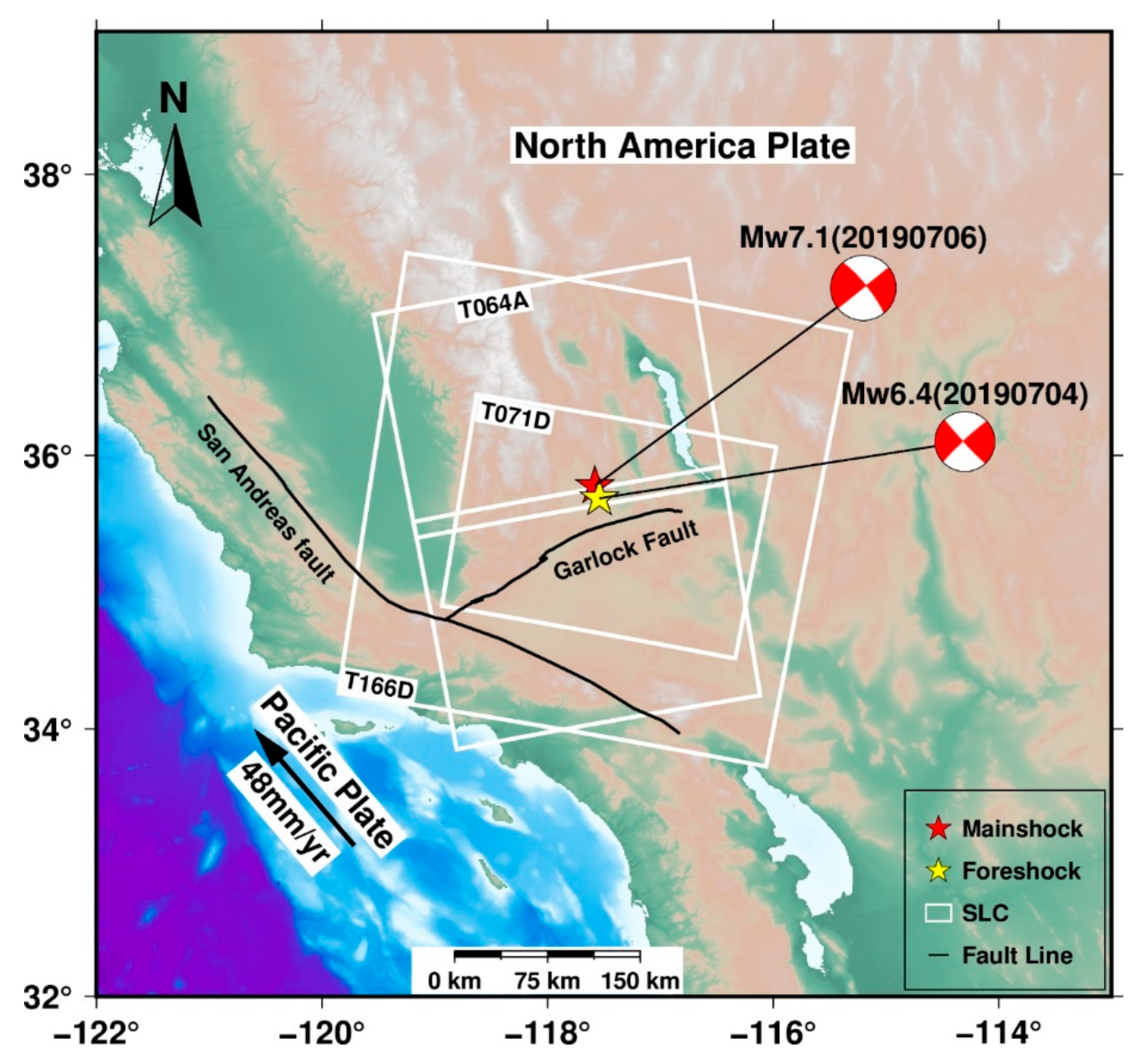
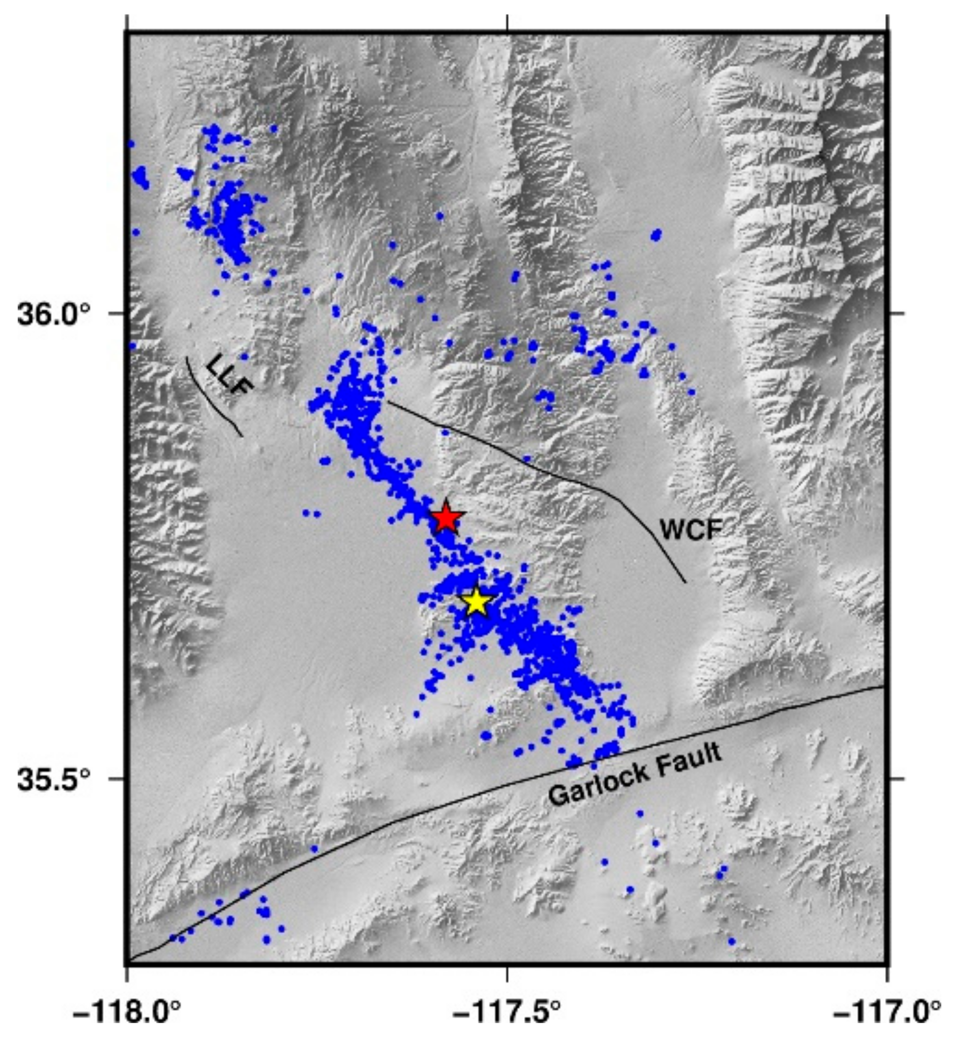
2. Geological Background

California, located in the western United States, is an earthquake-prone region with complex regional geology and active faults (Figure 1). The studied earthquakes occurred in the eastern California shear zone (ECSZ), which is part of the Pacific–North American plate boundary [10]. ECSZ was formed by a stress concentration resulting from a restraining bend in the San Andreas fault [11]. The regional geological structure is primarily strike-slip, and the primary faults in the area are the San Andreas fault, Garlock fault (GF), and Owens Valley fault. In addition, there are certain secondary faults, such as the Little Lake fault (LLF), Airport Lake fault, and Wilson Canyon fault (WCF), which overlap with each other to form complex geological settings. The San Andreas fault is located at the junction of the Pacific Plate and North American Plate. The Pacific Plate is one of the most seismically active faults in the world, and it is moving toward the North American Plate at a speed of 49 mm/yr [2]. The epicenter of the two earthquakes was located 10–20 km north of the Garlock fault, which is the boundary between the southern Mojave Desert and the Sierra Nevada and northern Nevada basin [12]. The Garlock Fault is one of the Holocene active faults in California, and it is 257 km long. According to report [13], the July 2019 seismic events included the strongest earthquake in this area for the past 20 years. This earthquake caused strong vibrations within 40 km of the epicenter, including in the city of Ridgecrest. It also caused several small-scale fires. Therefore, studying the earthquake geological structure and analyzing its post-seismic deformation is vital to understanding earthquake risks.

3. Materials and Methods

3.1. SAR Datasets

In this study, Sentinel-1A SAR images from the ESA and ALOS-2 PALSAR SAR images from JAXA were used. The coverage of the images is displayed in the white rectangles in Figure 1. To accurately obtain the co-seismic deformation of the two earthquakes, we used interferometric pairs from three tracks for the earthquake area. The detailed parameters of the interferometric pairs are listed in Table 2. Because the T064A and T071D master images were acquired on 4 July 2019, the interferograms of the two tracks include both the foreshock and mainshock deformations. We collected 27 SAR images from the ascending track (T064A) to study the post-seismic deformation mechanism. The timespan of the images was from 16 July 2019, to 15 August 2020. The detailed parameters are displayed in Table 3.

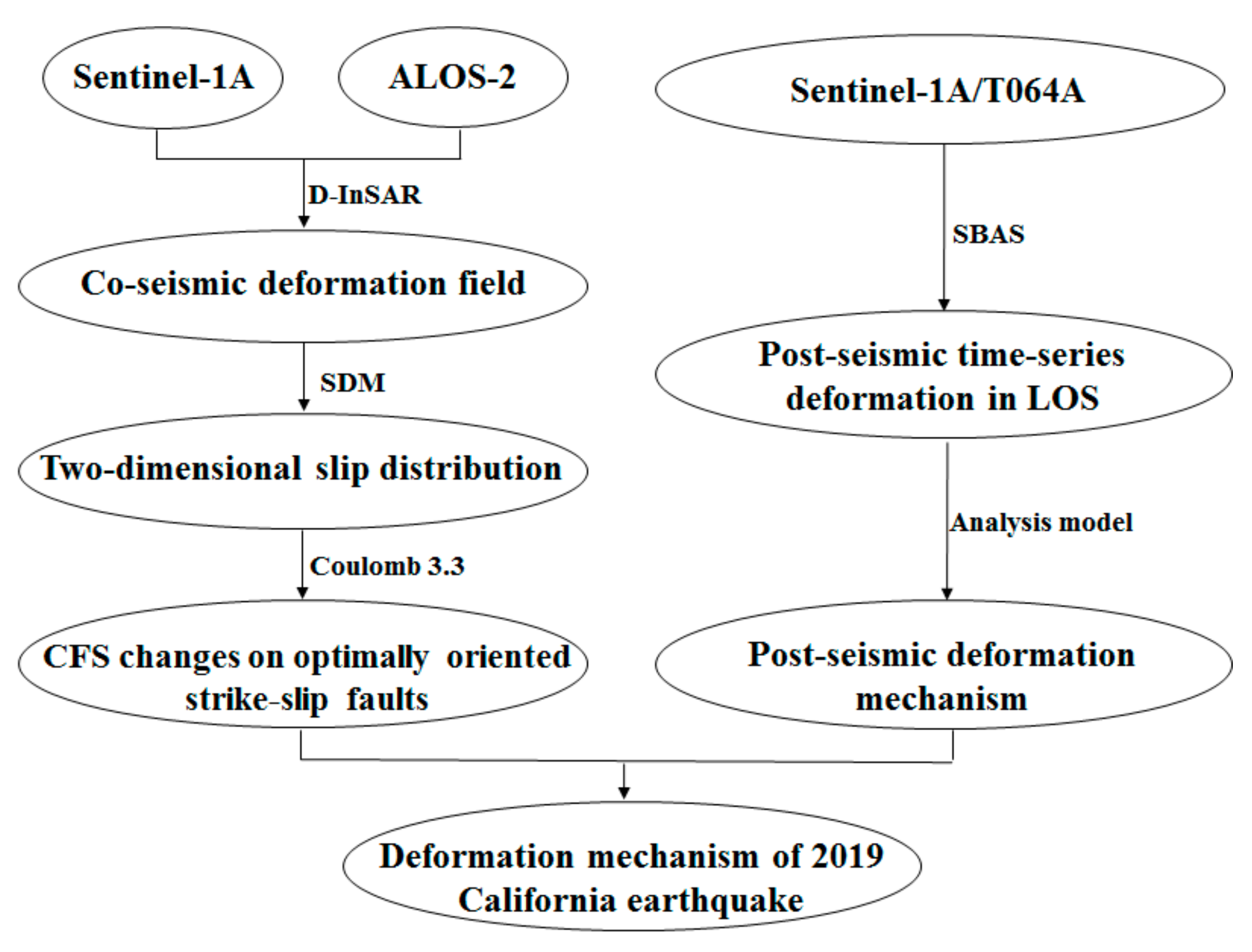
3.2. Data Processing

Based on GAMMA software [14], we used differential InSAR (D-InSAR) technology to obtain the co-seismic deformation fields. To improve the signal-to-noise ratio (SNR), interferograms were multi-looked by factors of eight in range and two in azimuth; the ground distance resolution of each pixel was approximately 29.48 × 27.88 m. The interferogram from ALOS-2 was multi-looked by factors of six in range and twenty-eight in azimuth, which was equal to a resolution of approximately 81.83 × 80.21 m. We used a shuttle radar topography mission digital elevation model with a 30 m resolution from the National Aeronautics and Space Administration to remove the topographic phase. All interferograms were filtered using an adaptive filter function based on the weighted power spectrum [15]. Phase unwrapping was performed using the minimum cost flow algorithm based on the Delaunay triangulation [16]. Observed phase nonlinear least-squares adjustments over stable areas were used to refine the nonlinear residual orbit error [17]. We also used the following model (Equation (1)), which was based on the correlation between the atmospheric delay phase and topography, to correct the atmospheric delay error [18]. Finally, the co-seismic deformation fields in the geographical coordinate system were obtained through geocoding.
φ a t m o = b 1 + b 2 * h g t x , y
where φ a t m o is the atmospheric delay phase, b 1 and b 2 are the undetermined coefficients, and h g t x , y is the point elevation.
To further analyze the post-seismic deformation characteristics, 27 Sentinel-1A images from the ascending track were processed using a small baseline subset (SBAS) [19,20]. The SAR images were divided into different subsets according to certain spatial and temporal baseline settings. Singular value decomposition was used to connect various differential interferogram subsets and to solve the time-series deformation at each coherent point. This method can weaken the DEM error and atmospheric phase delay of the deformation signals. The image data was from 28 July 2019, to 15 August 2020. The time and spatial baselines were no more than 100 d and 80 m, respectively. All interferograms were multi-looked by factors of six in range and one in azimuth. Interferogram filtering and unwrapping were performed using the same method as that of D-InSAR processing. The unwrapping was performed at points with a coherent value greater than 0.2. Interferograms with sufficient coherence, a continuous unwrapping phase, and a negligible atmospheric phase delay error were selected for the time-series deformation calculation. Figure 2 shows the flowchart of our research.

4. Results

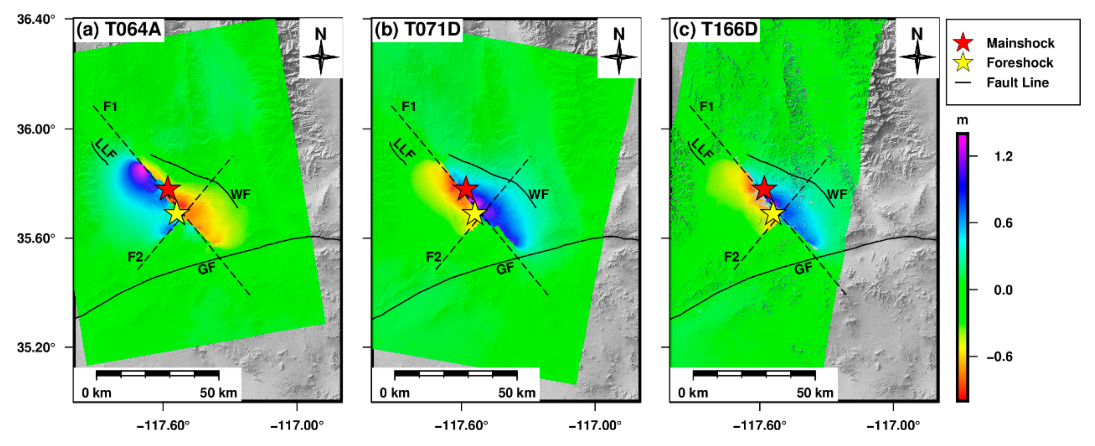
4.1. Co-Seismic Deformation Field

According to the processing settings described in Section 2, the co-seismic deformation fields were obtained from the Sentinel-1 and ALOS-2 SAR images (Figure 3). A positive value indicates that the deformation approached the satellite along the line of sight (LOS) (uplifting), and a negative value indicates that the deformation was moving away from the satellite along the LOS (subsiding). It can be seen from the co-seismic deformation field (Figure 3) that the ascending and descending interferograms covered the earthquake epicenter. The maximum uplift and subsidence deformations along the LOS were 1 and 0.71 m from the ascending track, respectively (Figure 3a). The co-seismic deformation fields from the descending tracks exhibited maximum uplift deformations of 1.3 and 1.4 m, which may be due to the difference of two master images. And the maximum subsidence ones were both 1 m (Figure 3b,c). The deformation fields from the ascending and descending tracks exhibited the opposite deformation trend, demonstrating that the co-seismic displacement was caused by significant horizontal displacement, which is consistent with the characteristics of a strike-slip fault structure [21,22]. The maximum uplift and subsidence of the co-seismic deformation monitored by Li et al. were 0.71 and 0.64 m, respectively, which are consistent with our results, indicating that our monitoring results are reliable.

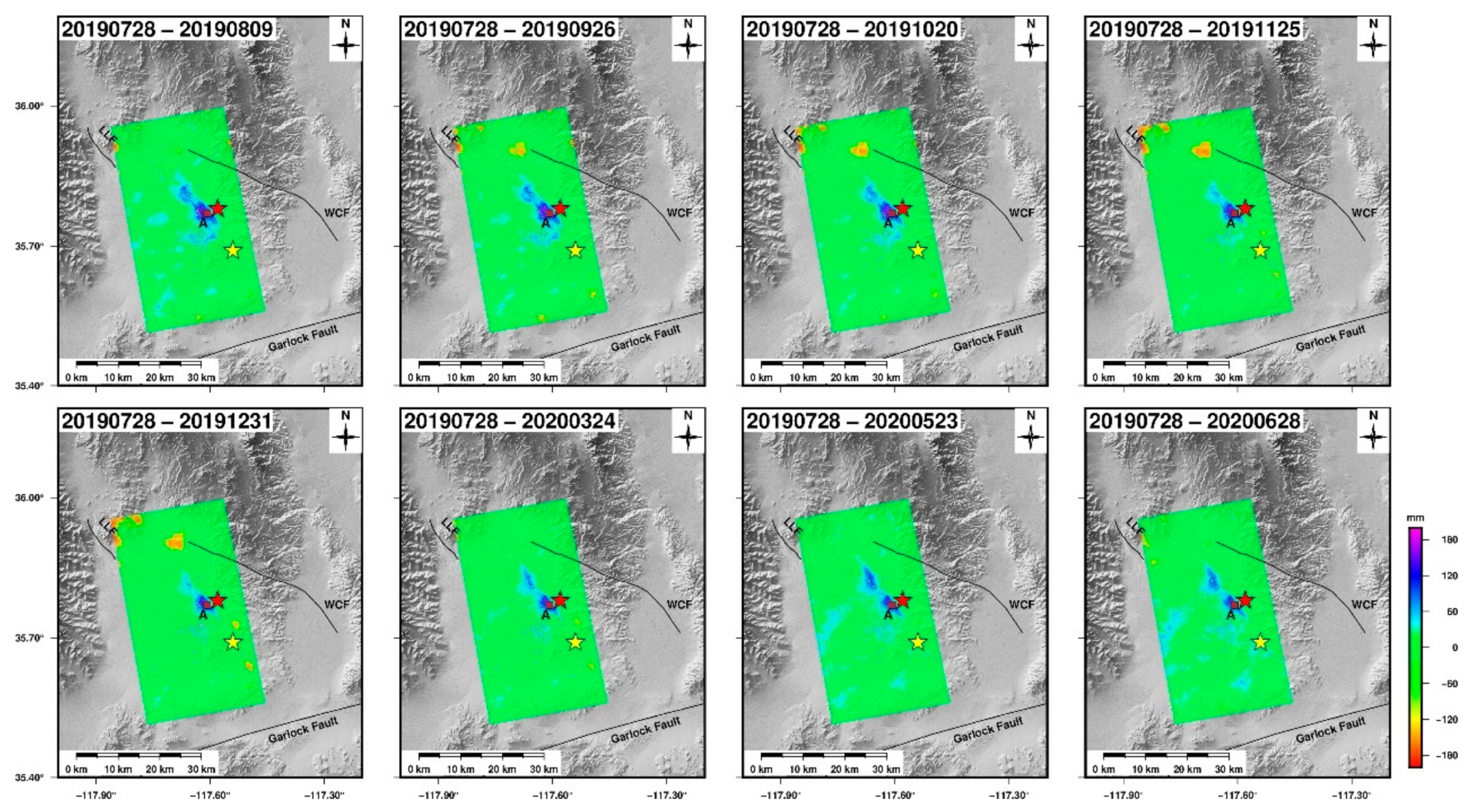
4.2. Post-Seismic Time-Series Deformation

Monitoring post-earthquake deformation can provide a critical basis for judging post-seismic deformation trend. To study the post-seismic deformation of the 2019 California earthquake, we investigated Sentinel-1A images covering the study area. Therefore, Sentinel-1A images in the ascending mode were used to calculate the post-earthquake deformation 402 d after the mainshock.
Previous studies [23,24] have illustrated that post-seismic deformations can be divided into three types: after-slip, poroelastic rebound, and viscoelastic relaxation. After-slip deformation occurs shortly after the earthquake. Poroelastic rebound primarily refers to the process where the pore water pressure gradient is generated by an earthquake, and the pore water is redistributed and balanced after the earthquake, causing crustal shrinkage or expansion. The earthquake altered the stress state of the viscous lower crust and upper mantle, which was subsequently released in a viscoelastic manner, acting on the upper crust to form significant surface deformation. Based on the observed surface deformation after the earthquake, a model can be constructed to invert the rheological structure of the lower crust and upper mantle, providing a basis for studying other dynamic processes. Viscoelastic relaxation, a large-scale deformation, often lasts several years after an earthquake.
We obtained the time-series deformation along the LOS from 28 July 2019, to 15 August 2020. Figure 4 displays a portion of the post-seismic deformation field. Conjoint analysis of co- and post-seismic deformation field demonstrated that the post-seismic deformation was smaller than the co-seismic deformation and that the post-seismic deformation primarily occurred near the epicenter. The movement direction of the post-seismic deformation was the same as that of the mainshock. Therefore, it was preliminarily determined that the post-seismic deformation mechanism was predominately after-slip.
The post-earthquake deformation is primarily concentrated at the junction of the co-seismic northwest–west (NWW) and southeast–east (SE–E) disks. –Therefore, we extracted the time-series deformation of point A at the junction to analyze the deformation trend 402 d after the mainshock. We used the following equation to fit the time-series deformation of point A [25,26]:
y = D + a × l o g 10 1 + t
where D is the initial main shock deformation (mm), a is the amplitude of the log function, t is the time interval after the mainshock (d), and y is the cumulative deformation (mm). The post-seismic deformation was set as the initial D value in Equation (3); D was set to 3.179, and a was set to 33.96. The fitting curve is illustrated by the red line in Figure 5.
From 28 July 2019, to 26 September 2019, and the cumulative deformation gradually increased. Over time, the deformation rate began to slow down. The post-seismic cumulative deformation of point A was 98 mm in the LOS.
According to previous research [23,27], we found that the after-slip typically occurs in the middle and upper 4 km of the fault. After the earthquake, the after-slip occurred quickly, and the deformation gradually shifted to a slow creep 100–300 d after the earthquake. Therefore, our observations support the hypothesis that after-slip can explain this post-seismic deformation mechanism more than poroelastic rebound or viscoelastic relaxation. We found that the number of aftershocks gradually decreased over time, indicating that the after-slip temporal evolution is consistent with that of the aftershocks of the California earthquake. With the decrease in the number of aftershocks, the after-slip also gradually weakened. The correlation coefficient between the frequency of aftershocks and the increase in post-earthquake deformation reached 0.91.

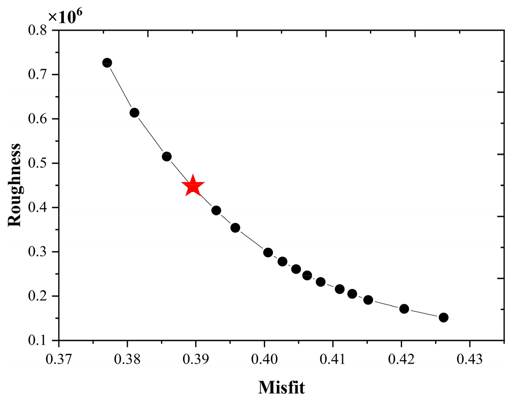
4.3. Co-Seismic Slip Distribution Inversion

Inverting the co-seismic deformation field is vital for understanding the mechanisms of earthquakes and regional activities. The co-seismic deformation field (Figure 3) demonstrates that there is an apparent deformation boundary to the SW. We also investigated 1581 earthquake recordings with Mw > 2.0, for the 402 d after the mainshock (Figure 6). The aftershock distribution also indicated that there was an apparent aftershock distribution boundary below the left of the deformation area. Therefore, this earthquake was not a single fault rupture but included at least two fault ruptures. This conclusion is consistent with the research results of Liu et al., Chen et al. and Milliner, Chris et al. [28]. Then, we outlined a fault model composed of SE–NW (F1) and southwest–northeast (SW–NE) (F2) intersecting faults (Figure 3). In this study, we used F1 and F2 to calculate the slip distribution on the faults and analyze the earthquake mechanism.
Because the timespans of the three co-seismic deformation fields were 12 d, 24 d, and 110 d, respectively, the co-seismic deformation fields not only included the foreshock deformation but also the co-seismic deformation. Because there is no suitable SAR image data for separating the mainshock and foreshock, the deformation fields of the mainshock and foreshock were not distinguished in our inversion. The steepest descent method (SDM) was used to calculate the optimal slip distribution [29,30]. This method was based on the Okada elastic half-space model, and the fault model was established according to the relevant parameters as follows:
y   =   f x   +  
where x is the related fault parameter, such as the length along the strike, width along the dip, location, strike, dip angle, and slip; y is the surface observation value; and is the error. After the fault source parameters were determined, the dislocation model inversion was transformed into a general linear inversion problem:
  y   =   G b   +  
where G is the Green function used to calculate the earth layered medium model, and b represents the fault slip along the strike and dip directions. To obtain a high-precision result, a fault is typically discretized into several patches, and the length and width of the fault are appropriately extended. For an inversion, the algorithm must be smoothed to avoid instability and other problems, and is the residual between the InSAR observation and SDM model.
In this inversion, we combined the ascending and descending observations and set the weight factor to 1:1:1 to invert the optimal slip distribution. The fault locations were set according to the co-seismic deformation field (Figure 3). The fault parameters were set according to the focal mechanism solution from the USGS. The F1 strike and dip angles were 322° and 83°, respectively. The F2 strike and dip angles were 225° and 81°, respectively. To improve the deformation fit, these parameters can increase to a certain degree of freedom in the inversion. We subsampled the ascending and descending datasets using uniform sampling and the quadtree method before performing the inversion. Quadtree sampling can alter the sampling point density according to the deformation gradient [31]. As a result, the quadtree method reduces the number of observation points while simultaneously guaranteeing the point density in places with substantial deformation gradients, thereby avoiding the loss of small deformation characteristics. To fully obtain the fault slip distribution, we expanded the fault along the strike direction and down the dip direction of F1 by 100 and 40 km, respectively, expanded those of F2 by 60 and 32 km, respectively, and set 4 × 4 km as the patch size. Finally, we divided the faults into 370 patches to calculate the co-seismic slip distribution. According to the focal mechanism solutions provided by several previous studies, we know that the earthquake was primarily strike-slip. The slip angle was constrained according to the strike-slip fault. To ensure stability and reduce the inversion uncertainty, a smoothing factor was introduced. The optimal smoothing factor was determined using an L-curve, as illustrated by the red star in Figure 7. Finally, we set the smoothing factor to 0.07. Figure 8 displays the co-seismic deformation inversion results, and the detailed inversion parameters are listed in Table 4.
The observation and prediction correlation was 0.93, and the residuals were predominately near zero. The results of the distributed slip inversion are displayed in Figure 9. The inversion results demonstrated that the earthquake caused a surface rupture. The distribution of the F1 co-seismic slip was primarily concentrated along strike between 24 and 76 km and at 0–20 km depth. The average rake was −171.83°, and the average slip was 0.4 m. The slip of fault F1 primarily exhibited right-lateral slip motion (Figure 9a). For F2, the co-seismic slip was primarily concentrated along strike between 16 and 34 km and at 0–14 km depth, with an average rake of 4.00° and an average slip of 0.13 m, indicating that F2 was predominately a left-lateral strike-slip (Figure 9b). When the shear modulus of the region was 30 GPa, the seismic moment magnitude obtained by SDM was Mw 7.08, which is consistent with the focal mechanism solution provided by USGS and GCMT and was similar to the results of Liu et al. and Barnhart et al.

5. Discussion

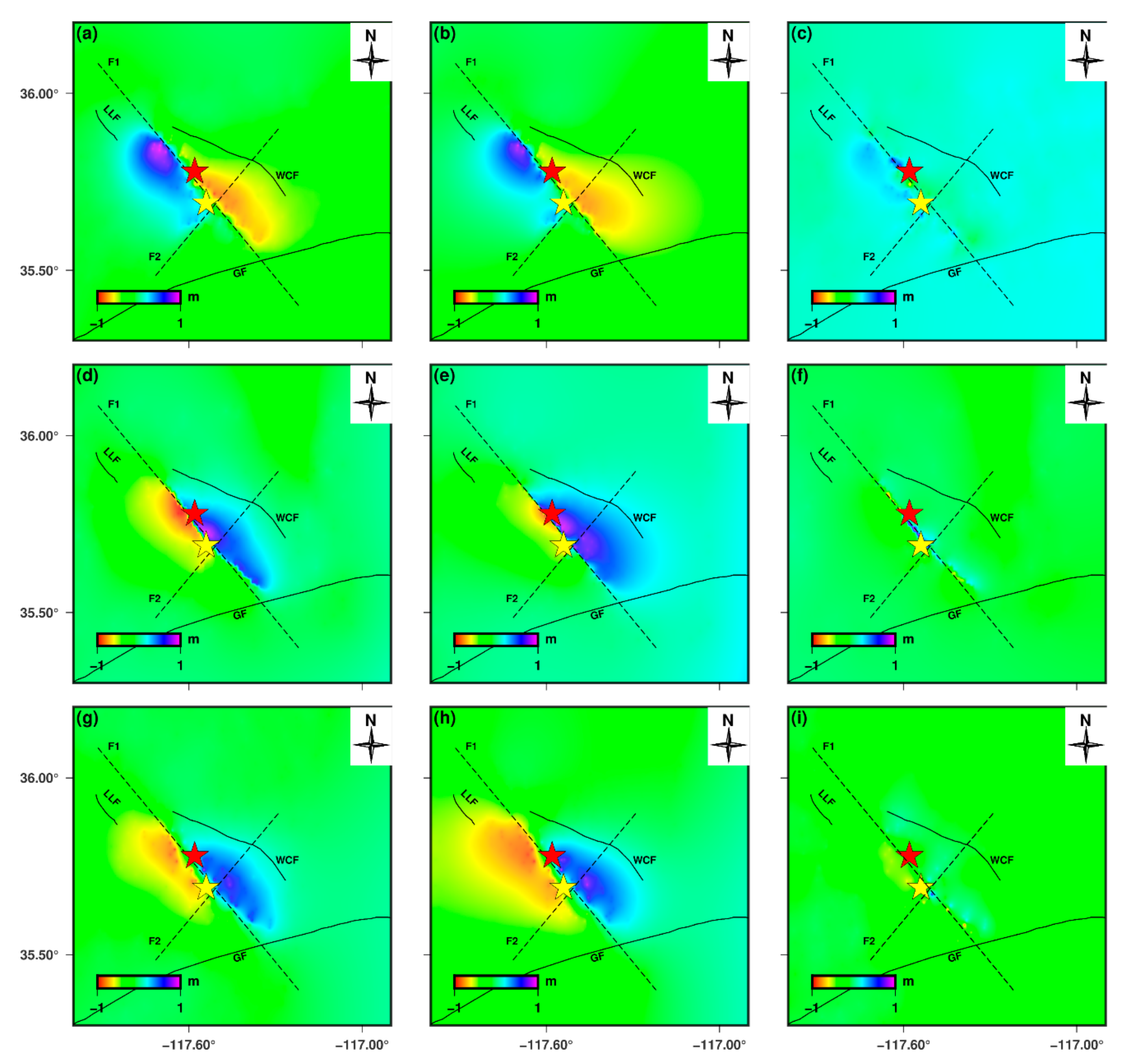
5.1. Coulomb Stress Change

The occurrence of a large earthquake causes a stress change on the regional faults around the focal area, affecting the seismicity [32,33]. Previous research has indicated that the mainshock can trigger strong aftershocks [34,35]. According to triggering theory, if the CFS is positive after an earthquake, it promotes fault rupture, and the corresponding seismic risk increases. In contrast, if the CFS is negative, it suppresses fault rupture and reduces seismic risk. The negative CFS area is called the “stress shadow area”. The slip distribution of the fault was obtained using SDM inversion. As a result, Coulomb stress can be calculated using the following formula:
Δ C F S   =   Δ τ r a k e + μ Δ σ n
where Δ τ r a k e is the static shear stress change in the fault and the sliding direction. Δ τ r a k e can be obtained based on the stress change tensor. μ is the effective fault friction coefficient on the receiving fault, which includes the pore fluid and medium characteristics of the fault. Δ σ n is normal stress change.
Based on the co-seismic slip distribution results, the fault rupture influence on the surrounding area was calculated using Coulomb3.3 software [36,37]. The relationship between the CFS and aftershock distribution was analyzed. We set the shear modulus to 30 GPa, the effective friction coefficient to 0.4. We selected the optimal strike-slip fault as the receiving fault. Using the co-seismic slip distribution results, we calculated the Coulomb stress changes at various projection depths. The Coulomb stress changes at depths of 5, 10, and 15 km are displayed in Figure 10. The released co-seismic moment was 4.3 × 1026, which is equivalent to Mw 7.06. According to a previous study [37], we know that the Coulomb stress field of a strike-slip earthquake is petal-shaped, which is consistent with our calculation results (Figure 10). If the Coulomb stress is greater than 0.1 bar, it can trigger subsequent aftershocks. Based on the calculation results, we found that the positive stress area was distributed along F1 and F2, and the stress shadow areas were roughly distributed in the NW–W, SE–E, and N–NW region. The maximum Coulomb stress was 3 bar and was located near F1. We found that aftershocks of Mw >3.0 were primarily distributed in the positive Coulomb stress area (Figure 10). However, certain aftershocks were located in negative Coulomb stress areas, such as the aftershocks on the WCF. This phenomenon demonstrated that the failure process of this earthquake was complex, and one stress triggering mechanism cannot fully explain the process. The aftershocks were distributed within the stress shadow area, which was related to many factors, such as fault failure geometry, dynamic stress triggering mechanism, and regional tectonic environment [38,39].

5.2. Co-Seismic and Post-Earthquake Activity Mechanism

We analyzed the co-seismic deformation field from three perspectives and found that the ascending and descending deformation trends were opposite of each other. This phenomenon demonstrates that the deformation caused by co-seismic deformation was primarily horizontal deformation that conformed to the characteristics of strike-slip earthquakes. Our inversion results presented as 2 conjugate faults system, which was consistent with the co-seismic deformation fields. Therefore, our results are reasonable.
The post-earthquake monitoring results illustrated that the surface deformation continued for 402 d after the earthquake. The post-earthquake surface deformation decreased over time. After fitting the post-seismic deformation, we found that it was consistent with the after-slip mechanism. And the number of aftershocks decreased. Therefore, we concluded that post-seismic deformation mechanism was mainly after-slip acting following investigated the aftershocks. Moreover, aftershocks were primarily distributed at the junction of the two deformation regions, and the post-seismic deformation was primarily distributed SW of the mainshock, which indicated that the accumulated energy between the earthquakes did not completely release during the mainshock but was gradually released in the aftershocks. All of the signs indicate that seismic activity is intense near the mainshock, and so closer attention should be paid to this region.

6. Conclusions

In this study, Sentinel-1A and ALOS-2 SAR images were used to obtain the co-seismic and post-seismic deformation fields of California earthquakes in July 2019. The co-seismic deformation was inverted using the Okada elastic half-space model. The surface deformation 402 d after the earthquake was assessed. The study conclusions are as follows.
  • The maximum uplift co-seismic deformation was 1.4 m in the LOS. The maximum subsidence co-seismic deformation was 1 m in the LOS. The deformation fields from the ascending and descending tracks exhibited the opposite deformation trend, which is consistent with the characteristics of a strike-slip fault. The co-seismic deformation fields demonstrated that this earthquake event was caused by the ruptures of at least two faults. Multi-faults model was used in the inversion.
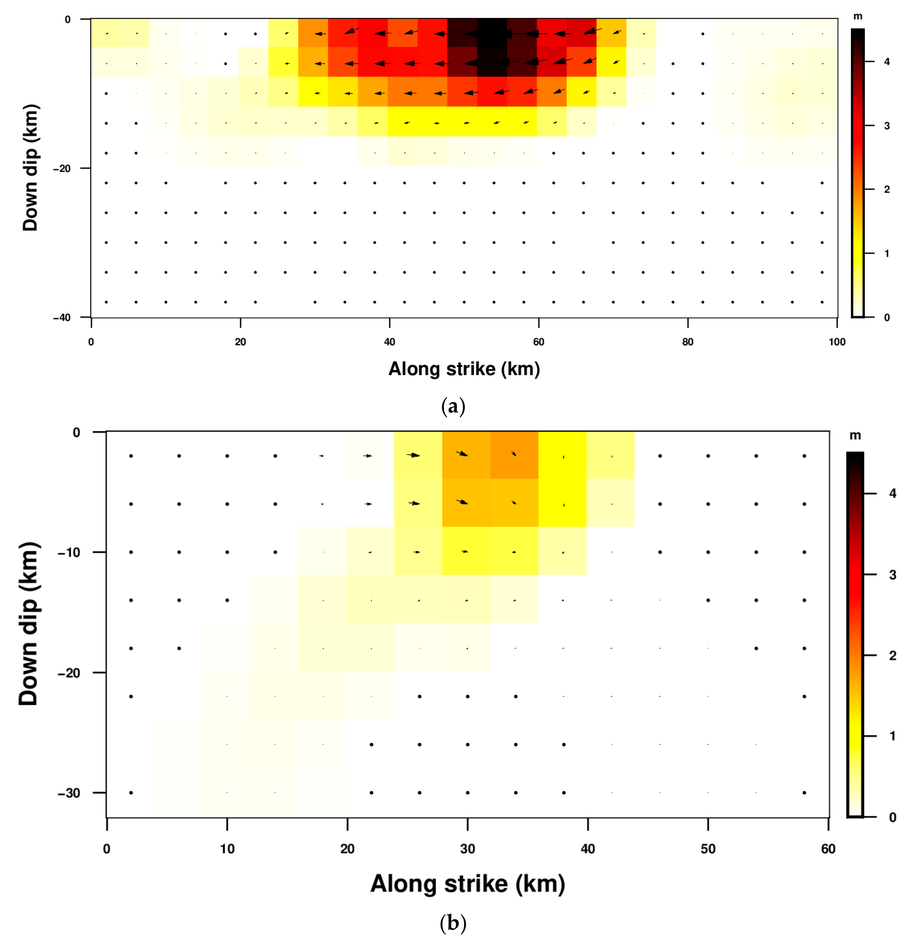
  • The co-seismic slip distribution inversion illustrates that F1 was dominated by a right-lateral strike-slip, the average rake was −171.83°, and the average slip was 0.4 m. F2 was dominated by a left-lateral strike-slip, the average rake was 4°, and the average slip was 0.13 m. The magnitude of this earthquake was approximately Mw 7.08. This California earthquake was a strike-slip fault event.
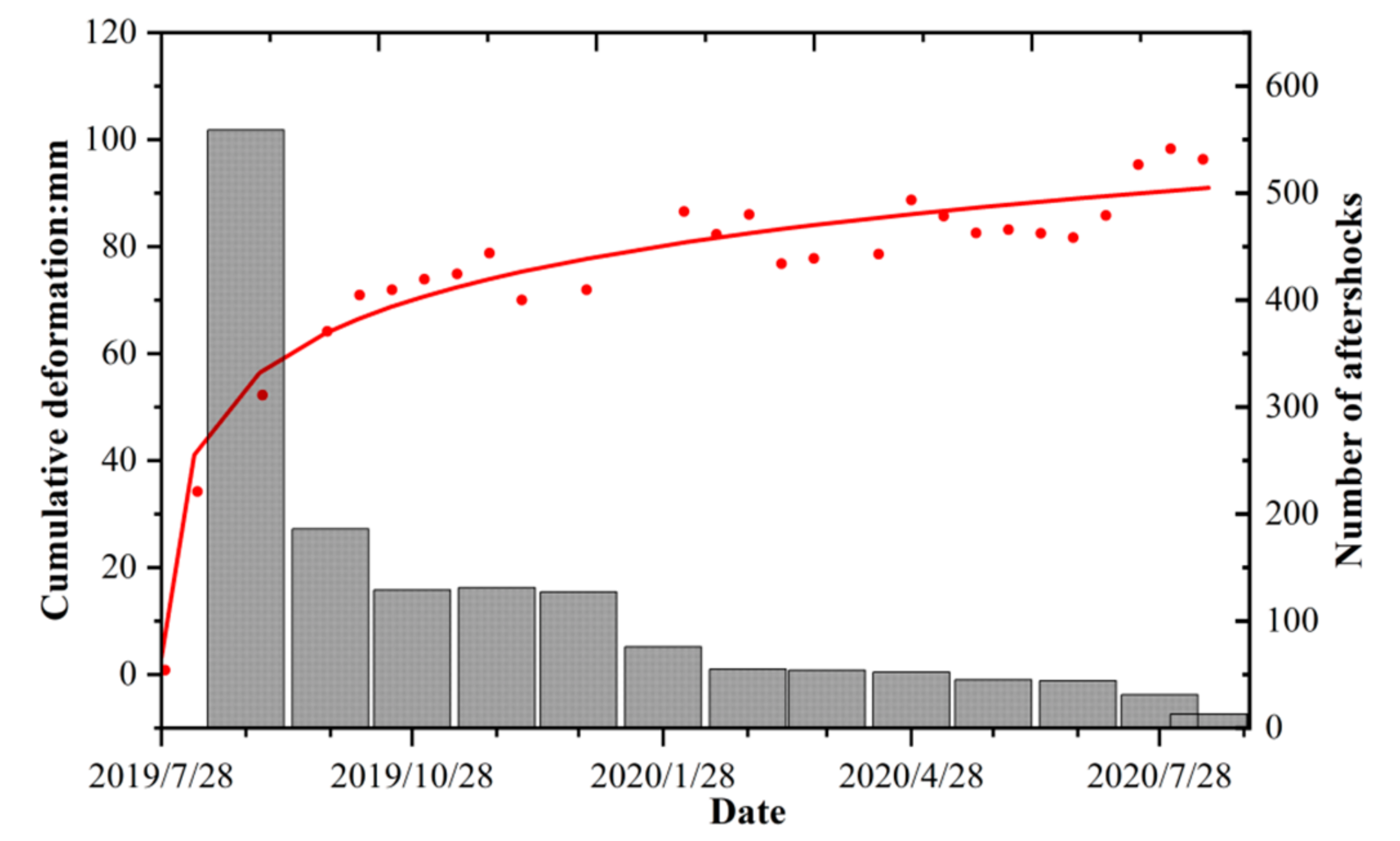
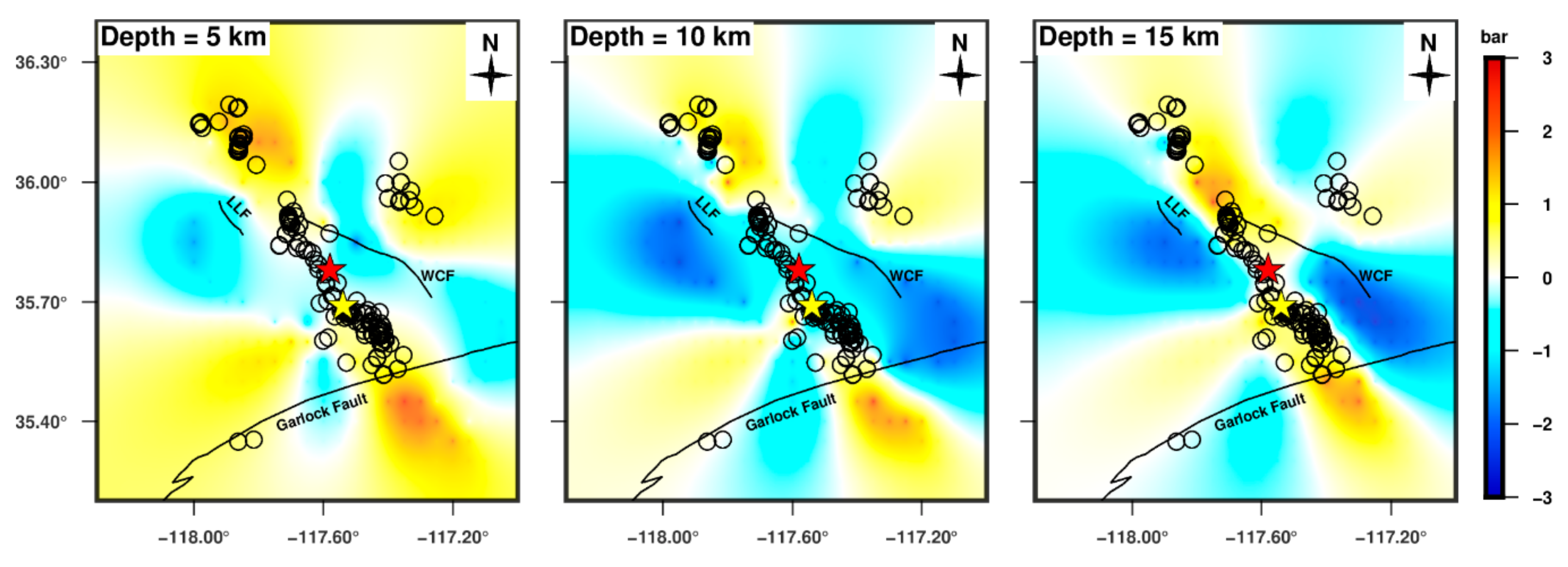
  • The post-seismic deformation typically occurs near the epicenter. After 402 d, the post-earthquake deformation gradually tends to be stable. The post-seismic deformation mechanism of this earthquake was primarily after-slip. The calculation of the Coulomb stress change exhibits that the co-seismic moment released by the earthquake was approximately 4.24 × 1026 N × m, which is equivalent to a moment magnitude of 7.06. This finding is consistent with the co-seismic slip distribution inversion results. The maximum Coulomb stress was located near F1. However, certain aftershocks were located in negative Coulomb stress areas. Therefore, the failure process of this earthquake was complex.
In a nutshell, this earthquake event was a strike-slip fault event, and caused by the ruptures of at least two faults, with different strike-slip directions. The post-earthquake deformation showed after-slip and gradually becomes stable in the 400 days after the earthquake.

Author Contributions

S.Z. and C.Y. conceived and designed the experiments; T.W. performed the experiments and drafted the manuscript; J.D. and B.H. contributed to the inversion and coulomb stress; C.Z. contributed to the InSAR data analysis. All authors have read and agreed to the published version of the manuscript.

Funding

This research was funded jointly by China Geological Disaster Investigation Project (DD20190637), the National Natural Science Foundation of China (NSFC) (No. 41731066), State’s Key Project of Research and Development Plan (2018YFC1504805).

Institutional Review Board Statement

Not applicable.

Informed Consent Statement

Not applicable.

Data Availability Statement

The data used to support the findings of this study are available from the corresponding author upon request.

Acknowledgments

We acknowledge the European Space Agency (ESA) for freely making available the Sentinel-1A data and ALOS-2 PALSAR from JAXA. Maps were prepared using the Generic Mapping Tools (GMT) and Origin software.

Conflicts of Interest

The authors declare no conflict of interest.

References

  1. Li, S.; Chen, G.; Tao, T.; He, P.; Ding, K.; Zou, R.; Li, J.; Wang, Q. The 2019 MW 6.4 and Mw 7.1 Ridgecrest Earthquake Sequence in Eastern California: Rupture on a Conjugate Fault Structure Revealed by GPS and InSAR Measurements. Geophys. J. Int. 2020, 221, 1651–1666. [Google Scholar] [CrossRef]
  2. Chen, K.; Avouac, J.-P.; Aati, S.; Milliner, C.; Zheng, F.; Shi, C. Cascading and Pulse-Like Ruptures During the 2019 Ridgecrest Earthquakes in the Eastern California Shear Zone. Nat. Commun. 2020, 11, 1–8. [Google Scholar] [CrossRef]
  3. Barnhart, W.D.; Hayes, G.P.; Gold, R.D. The July 2019 Ridgecrest, California, Earthquake Sequence: Kinematics of Slip and Stressing in Cross-Fault Ruptures. Geophys. Res. Lett. 2019, 46, 11859–11867. [Google Scholar] [CrossRef]
  4. Liu, C.; Lay, T.; Brodsky, E.E.; Dascher-Cousineau, K.; Xiong, X. Emily Co-seismic Rupture Process of the Large 2019 Ridgecrest Earthquakes from Joint Inversion of Geodetic and Seismological Observations. Geophys. Res. Lett. 2019, 46, 11820–11829. [Google Scholar] [CrossRef]
  5. Shan, X.J.; Qu, C.Y.; Song, X.G.; Zhang, G.F.; Liu, Y.H.; Guo, L.M.; Zhang, G.H.; Li, W.D. Co-seismic deformation field observation and study of Wenchuan Ms8.0 earthquake by InSAR. J. Geophys. 2009, 52, 496–504. [Google Scholar]
  6. Xu, C.J.; Wang, L.Y. Research progress of seismic source rupture process by joint inversion of geodesy and seismic data. J. Wuhan Univ. (Inf. Sci.) 2010, 35, 457–462. [Google Scholar]
  7. Wang, C.S.; Shan, X.J.; Wang, C.L.; Ding, X.L.; Zhang, G.D.; Timothy, M. Using finite element and Okada models to invert co-seismic slip of the 2008 Mw 7.2 Yutian earthquake, China, from InSAR data. J. Seismol. 2013, 17, 347–360. [Google Scholar] [CrossRef]
  8. Li, N.; Zhao, Q.; Sun, H. InSAR observation of the 2015 Ms 7.4 earthquake in Tajikistan and its tectonic significance. Geod. Geodyn. 2018, 38, 43–47. [Google Scholar]
  9. Niu, Y.F.; Wang, S.; Zhu, W.; Zhang, Q.; Lu, Z.; Zhao, C.Y.; Qu, W. The 2014 Mw 6.1 Ludian Earthquake: The Application of RADARSAT-2 SAR Interferometry and GPS for this Conjugated Ruptured Event. Remote Sens. 2019, 12, 99. [Google Scholar] [CrossRef] [Green Version]
  10. Oskin, M.; Iriondo, A. Large-Magnitude Transient Strain Accumulation on the Blackwater Fault, Eastern California Shear Zone. Geology 2004, 32, 313. [Google Scholar] [CrossRef]
  11. Dokka, R.K.; Travis, C.J. Role of the Eastern California Shear Zone in Accommodating Pacific-North American Plate Motion. Geophys. Res. Lett. 1990, 17, 1323–1326. [Google Scholar] [CrossRef]
  12. Feng, W.; Samsonov, S.; Qiu, Q.; Wang, Y.; Zhang, P.; Li, T.; Zheng, W. Orthogonal Fault Rupture and Rapid Postseismic Deformation Following 2019 Ridgecrest, California, Earthquake Sequence Revealed from Geodetic Observations. Geophys. Res. Lett. 2020, 47, e2019GL086888. [Google Scholar] [CrossRef]
  13. Jennifer Andrews. Searles Valley Sequence: M6.4 and M7.1, Southern California Seismic Network. Available online: http://www.scsn.org/index.php/2019/07/04/07-04-2019-searles-valley-sequence/index.html (accessed on 15 June 2020).
  14. Werner, C.; Wegmuller, U.; Strozzi, T.; Wiesmann, A. Gamma SAR and Interferometric Processing Software. In Proceedings of the Ers-Envisat Symposium, Gothenburg, Sweden, 15–20 October 2000. [Google Scholar]
  15. Goldstein, R.M.; Werner, C.L. Radar Interferogram Filtering for Geophysical Applications. Geophys. Res. Lett. 1998, 25, 4035–4038. [Google Scholar] [CrossRef] [Green Version]
  16. Eineder, M.; Hubig, M.; Milcke, B. Unwrapping Large Interferograms Using the Minimum Cost Flow Algorithm. In Proceedings of the IEEE International Geoscience & Remote Sensing Symposium, Seattle, WA, USA, 6–10 July 1998; IEEE Publications: New York, NY, USA, 1998; p. 1998. [Google Scholar]
  17. Rosen, P.A.; Hensley, S.; Zebker, H.A.; Webb, F.H.; Fielding, E.J. Surface Deformation and Coherence Measurements of Kilauea Volcano, Hawaii, From SIR-C Radar Interferometry. J. Geophys. Res. 1996, 101, 23109–23125. [Google Scholar] [CrossRef]
  18. Yang, C.-S.; Zhang, Q.; Qu, F.-F.; Zhang, J. Obtaining an Atmospheric Delay Correction for Differential SAR Interferograms Based on Regression Analysis of the Atmospheric Delay Phase. Shanghai Land Resour. 2012, 3, 412. (In Chinese) [Google Scholar]
  19. Berardino, P.; Fornaro, G.; Lanari, R.; Sansosti, E. A New Algorithm for Surface Deformation Monitoring Based on Small Baseline Differential SAR Interferograms. IEEE Trans. Geosci. Remote Sens. 2002, 40, 2375–2383. [Google Scholar] [CrossRef] [Green Version]
  20. Lanari, R.; Mora, O.; Manunta, M.; Mallorqui, J.J.; Berardino, P.; Sansosti, E. A Small-Baseline Approach for Investigating Deformations on Full-Resolution Differential SAR Interferograms. IEEE Trans. Geosci. Remote Sens. 2004, 42, 1377–1386. [Google Scholar] [CrossRef]
  21. Shan, X.J.; Qu, C.; Gong, W.Y.; Zhao, D.Z.; Zhang, Y.F.; Zhang, G.H.; Song, X.G.; Liu, Y.H.; Zhang, G.F. Co-seismic deformation field of the Jiuzhaigou Ms7.0 earthquake from Sentinel-1A InSAR data and fault slip inversion. Chin. J. Geophys. (Chin.) 2017, 60, 4527–4536. [Google Scholar] [CrossRef]
  22. Ji, L.Y.; Liu, C.J.; Xu, J.; Liu, L.; Long, F.; Zhang, Z.W. InSAR observation and inversion of the seismogenic fault for the 2017 Jiuzhaigou Ms 7.0 earthquake in China. Chin. J. Geophys. 2017, 60, 4069–4082. (In Chinese) [Google Scholar] [CrossRef]
  23. Tan, K.; Wang, Q.; Wang, X.Q.; Yang, S.; Li, J. Analysis Model and Space Time Distribution of Post-seismic Deformation. J. Geod. Geodyn. 2005, 25, 23–26. (In Chinese) [Google Scholar]
  24. Ji, L.; Zhu, L.; Li, N.; Wang, C.Z. Research review of fault movement based on Geodetic observation. J. Geod. Geodyn. 2017, 37, 771–776. (In Chinese) [Google Scholar]
  25. Freed, A.M. Afterslip (and Only Afterslip) Following the 2004 Parkfield, California, Earthquake. Geophys. Res. Lett. 2007, 34, L06312. [Google Scholar] [CrossRef] [Green Version]
  26. Barnhart, W.D.; Brengman, C.M.J.; Li, S.; Peterson, K.E. Ramp-Flat Basement Structures of the Zagros Mountains Inferred From Co-Seismic Slip and After-slip of the 2017 MW 7.3 Darbandikhan, Iran/Iraq Earthquake. Earth Planet. Sci. Lett. 2018, 49, 96–107. [Google Scholar] [CrossRef]
  27. Marone, C.J.; Scholtz, C.H.; Bilham, R. On the mechanics of earthquake afterslip. J. Geophys. Res. 1991, 96, 8441–8452. [Google Scholar] [CrossRef]
  28. Milliner, C.; Donnellan, A. Using Daily Observations from Planet Labs Satellite Imagery to Separate the Surface Deformation between the 4 July Mw 6.4 Foreshock and 5 July Mw 7.1 Mainshock during the 2019 Ridgecrest Earthquake Sequence. Seismol. Res. Lett. 2020, 91, 1986–1997. [Google Scholar] [CrossRef]
  29. Wang, R.J.; Diao, F.; Hoechner, A. SDM-A Geodetic Inversion Code Incorporating with Layered Crust Structure and Curved Fault Geometry. In Proceedings of the EGU General Assembly, Vienna, Austria, 7–12 April 2013; European Geosciences Union: Munich, Germany, 2013. [Google Scholar]
  30. Wang, R.J.; Parolai, S.; Ge, M.; Jin, M.; Walter, T.R.; Zschau, J. The 2011 Mw9.0 Tohoku Earthquake: Comparison of GPS and Strong-Motion Data. Bull. Seism. Soc. Am. 2013, 103, 1336–1347. [Google Scholar] [CrossRef]
  31. Lohman, R.B.; Simons, M. Some thoughts on the use of InSAR data to constrain models of surface deformation: Noise structure and data downsampling. Geochem. Geophys. Geosyst. 2005, 6, Q01007. [Google Scholar] [CrossRef]
  32. King, G.C.P.; Stein, R.S.; Lin, J. Static Stress changes and the Triggering of Earthquakes. Bull. Seism. Soc. Am. 1994, 84, 935–953. [Google Scholar]
  33. Pinar, A.; Honkura, Y.; Kuge, K. Seismic Activity Triggered by the 1999 Izmit Earthquake and Its Implications for the Assessment of Future Seismic Risk. Geophys. J. Int. 2001, 146, F1–F7. [Google Scholar] [CrossRef] [Green Version]
  34. Liu, G.P.; Fu, Z.X. The Triggering Mechanism of the Largest Aftershock (Ms = 6.3) of the. Luhuo Gr. Earthquake (Ms =7.6). Earthq. Res. China 2002, 18, 175–182. (In Chinese) [Google Scholar]
  35. Wan, Y.G.; Wu, Z.L.; Zhou, G.W.; Huang, J.; Qin, L.X. Research on Seismic Stress Triggering. Acta Seism. 2002, 24, 533–551. (In Chinese) [Google Scholar] [CrossRef]
  36. Toda, S.; Stein, R.S.; Richards-Dinger, K.; Bozkurt, S.B. Forecasting the evolution of seismicity in southern California: Animations built on earthquake stress transfer. J. Geophys. Res. 2005, 110, B05S16. [Google Scholar] [CrossRef]
  37. Lin, J.; Stein, R.S. Stress triggering in thrust and subduction earthquakes, and stress interaction between the southern San Andreas and nearby thrust and strike-slip faults. J. Geophys. Res. 2004, 109, B02303. [Google Scholar] [CrossRef] [Green Version]
  38. Felzer, K.R.; Becker, T.W.; Abercrombie, R.E.; Ekström, G.; Rice, J.R. Triggering of the 1999 Mw7.1 Hector Mine earthquake by aftershocks of the 1992 Mw7.3 Landers earthquake. J. Geophys. Res. 2002, 107, 6–13. [Google Scholar]
  39. Steacy, S.; Marsan, D.; Nalbant, S.S.; Mccloskey, J. Sensitivity of static stress calculations to the earthquake slip distribution. Geophys. Res. 2004, 109, B04303. [Google Scholar] [CrossRef] [Green Version]
Figure 1. Study area tectonic setting. Red star represents mainshock epicenter, yellow star represents foreshock epicenter, and red and white circles represent the mainshock and foreshock focal mechanism solutions (from www.globalcmt.org (accessed on 3 February 2021)). The white rectangles mark the coverage of the synthetic aperture radar (SAR) images.
Remotesensing 13 00608 g001
Figure 2. The research process of our manuscript.
Remotesensing 13 00608 g002
Figure 3. Co-seismic deformation fields obtained from ascending and descending tracks. (a) for Sentinel-1A T064A, (b) for Sentinel-1A T071D, (c) for ALOS-2 T166D. Black lines indicate faults. Red and yellow stars indicate the mainshock and foreshock, respectively. Dotted line indicates inversion fault model.
Remotesensing 13 00608 g003
Figure 4. Partial post-seismic time-series deformation in line of sight (LOS). Red and yellow stars represent mainshock and foreshock, respectively.
Remotesensing 13 00608 g004
Figure 5. Time series of the cumulative deformation. Red points represent the cumulative deformation time series of the post-seismic. Red line represents fitting line of the post-seismic deformation. X-axis represents date, left Y-axis represents cumulative deformation in LOS, right Y-axis represents number of aftershocks.
Remotesensing 13 00608 g005
Figure 6. Mw 7.1 earthquake aftershock distribution. Red star is mainshock. Yellow star is foreshock. Blue dots indicate aftershocks of Mw > 2 (from 28 July 2019, to 15 August 2020).
Remotesensing 13 00608 g006
Figure 7. Curve representing tradeoff between model roughness and misfit. Red star indicates optimal smoothing parameter.
Remotesensing 13 00608 g007
Figure 8. Comparison between co-seismic deformation observations and distributed slip model of 2019 California earthquake. Red and yellow stars are mainshock and foreshock, respectively. (a) Observation, (b) prediction, and (c) residual from Sentinel-1A (T064A). (d) Observation, (e) prediction, and (f) residual from Sentinel-1A (T071D). (g) Observation, (h) prediction, and (i) residual from ALOS-2 (T166D).
Remotesensing 13 00608 g008
Figure 9. Two-dimensional optimal slip distributions of (a) F1 and (b) F2. The heading of the black arrows indicates the slip vectors of each patches.
Remotesensing 13 00608 g009
Figure 10. CFS changes on optimally oriented strike-slip faults at depths of 5, 10, and 15 km. Red and yellow stars are mainshock and foreshock, respectively. Black circles represent aftershocks (Mw > 3) for 402 d after mainshock.
Remotesensing 13 00608 g010
Table 1. Focal mechanism solutions for 2019 California earthquakes.
DateLongitude (°E) Latitude (°N)Np1 (Strike, Dip, and Rake)Np2 (Strike, Dip, and Rake)
USGS a2019.7.4−117.50435.705228/66/4137/86/156
2019.7.6−117.59935.770322/81/−173231/83/−9
GCMT b2019.7.4−117.5435.69227/86/3137/87/176
2019.7.6−117.5835.780321/81/18051/90/9
William D. Barnhart et al.7.4--228/66/4
7.6--322/81/−173
Li et al.Fault 1--320/83/−171
Fault 2--225/81/−
This studyFault 1--322/83/−172
Fault 2--225/81/4
a—USGS: United States Geological Survey (https://earthquake.usgs.gov/); b—GCMT: Global Centroid Moment Tensor Catalogue (https://www.globalcmt.org/ (accessed on 3 February 2021)). For Fault 1 and Fault 2 refer to the tectonic faults divided by the authors.
Table 2. Co-seismic interference pair parameters.
No.SatelliteOrbitPass
Direction
Master
Image
Slave
Image
IntervalIncidence
Angle
Perpendicular Baseline
1Sentinel-1AT064Ascending 20190704201907161239.2582−27.4
2Sentinel-1AT071 Descending20190704201907282439.2026−40.5
3ALOS-2T166Descending201904022019072311239.0301−496.9
Table 3. Details of selected aftershock interference pairs.
OrbitPass DirectionIncidence AngleHeadingNumber of ImagesNumber of Interferograms Involved in Calculation
T064A
(Sentinel-1A)
Ascending39.2582−12.992739
Table 4. California earthquake inversion parameters.
FaultMean RakeMean SlipLatitudeLongitudeDepth
F1−171.830.4035.77−117.591.99
F24.000.1335.67−117.531.98
Publisher’s Note: MDPI stays neutral with regard to jurisdictional claims in published maps and institutional affiliations.

