
Determination of Process Noise for Underwater Target Tracking with Forward Looking Sonar


Faculty of Navigation, Chair of Geoinformatics, Maritime University of Szczecin, 70-500 Szczecin, Poland
*
Author to whom correspondence should be addressed.
Remote Sens. 2021, 13(5), 1014; https://0-doi-org.brum.beds.ac.uk/10.3390/rs13051014
Submission received: 6 February 2021
/
Revised: 28 February 2021
/
Accepted: 4 March 2021
/
Published: 8 March 2021
(This article belongs to the Special Issue 2nd Edition Radar and Sonar Imaging and Processing)
Abstract
:Target tracking is a process that provides information about targets in a specific area and is one of the key issues affecting the safety of any vehicle navigating in water. The main sensor used for underwater target tracking is sonar, with one of the most popular configurations being forward looking sonar (FLS). The target tracking state vector is usually estimated with the use of numerical filter algorithms, such as the Kalman filter (KF) and its modification, or the particle filter (PF). This requires the definition of a process model, including process noise, and a measurement model. This study focused on process noise definition. It is usually implemented as Gaussian noise, with a covariance matrix defined by the author. An analytical and empirical analysis was conducted, including a verification of the existing approaches and a survey of the published literature. Additionally, a theoretical analysis of the factors influencing process noise was conducted, which was followed by an empirical verification. The results were discussed, leading to the conclusions. The results of the theoretical analysis were confirmed by the empirical experiment and the results were compared with commonly used values of process noise in underwater target tracking processes.

1. Introduction
Underwater target tracking using underwater acoustic methods has become a hot topic in both industrial and scientific research. A wide variety of applications, mainly based on various configurations of sonar sensors and dedicated for different purposes, have been proposed. One important application is collision avoidance for autonomous underwater vehicles (AUV) or remotely operating vehicles (ROV). According to [1], AUVs have the potential to revolutionize human underwater activities and the improvement of their navigation is one of the primary challenges in AUV research today. Similar conclusions were attained by [2], where underwater sensors were found to be an obvious source of information for the navigation of autonomous surface vehicles (ASV), expanding the use of sonar for navigation purposes. Target tracking plays an important role in the safe navigation of autonomous vehicles. Other important applications of underwater target tracking were presented by [3], together with a review of the methods used. In general, there are three basic sensor configurations for underwater target tracking based on acoustic imaging sensors: forward looking sonar (FLS), traditional acoustic sensor arrays (TASAs) and underwater wireless sensor networks (UWSNs). The empirical research in this study was performed with the use of FLS; however, the results can be easily extrapolated to other sensor configurations.
The essence of underwater target tracking is to estimate the state vector of a target detected underwater through the use of acoustic waves. This determines the originality of the process compared to other tracking applications. As indicated by [3], the underwater environment causes specific propagation and communication conditions, which have to be included. For most applications, 3D real time tracking is also expected, which has an influence on the tracking method itself. Nevertheless, although the sensor modes and configurations may be different, the numerical basics of the tracking algorithms are the same because they use the same filters, mostly various modifications of the Kalman filter (KF) or particle filter (PF). The goal is always to sequentially estimate the target parameters from the sensor observations. The system state vector usually contains information about the location, course, and speed of the target and the observations may be the signal strength, bearing, and arrival time of the returned signal [4]. The fine taxonomy used in underwater tracking algorithms is given in [3]. The systems can be classified according to the sensor configuration, as mentioned before, but also according to the mode-based method (active, passive) and the tracking optimization method (noise driven, source driven). In this study, we focused on active tracking with filtering as a noise driven optimization method. This approach is met in most applications based on underwater imaging sensors.
Although the sensors used are different, underwater tracking process algorithms are similar to those used in radar target tracking for anti-collision purposes. Therefore these applications may also be used as a source of information for the development of underwater sensors. In the case of autonomous vehicles, other sensors used for collision avoidance include radars [5] and in some studies, e.g., [6], collision avoidance has been achieved by more adaptive path planning rather than the tracking of moving targets. To understand such anti-collision issues, precise information about the bathymetry is required [7] and the process then becomes a simultaneous localization and mapping (SLAM) problem, which is often met in robotic applications [8].
In general, underwater tracking is modeled with a system state process, which describes the evolution of the system in time (Equation (1)), and the measurement process, often called the observation process, can be modeled with Equation (2) [4]:
where: xk—n—dimensional state vector; zk+1—measurement vector; Uk—p—dimensional control (known external input) vector; Wk—state noise vector, Vk—measurement noise vector, k–discrete time.
In both models the noises are assumed to be independent random vectors with known statistics.
The tracking process results in an iterative prediction and correction of state with updated measurements. Because the most popular filters used for underwater target tracking are various modifications of the KF, they are reviewed in a later section. The importance of noise modeling should be realized. Measurement noise has a direct impact on the quality of measurements in models. It is usually derived from sensor characteristics and configurations. Process noise (often called transition noise) describes all the other factors that can influence or disturb the process. The value of the noise has a crucial meaning for assessing the quality of the tracking. Its magnitude is indicated by state vector covariance and is a consequence of the weighting between the measurement and prediction in the final estimation. Process noise is usually modeled with a noise covariance matrix. In underwater target tracking it usually contains the values of unknown accelerations caused mostly by environmental conditions. From the literature review, it was apparent that values are usually arbitrarily selected and are small but non-zero; however, there has been no attempt to justify their value in previous studies.
The main aim of this study was to determine the process noise in underwater target tracking FLS systems through a theoretical analysis and subsequent empirical verification. This should lead to confirmation or verification of the values presented in the literature. The main contribution of this paper is therefore the provision of discussion and conclusions on setting the noise model in numerical filters for sonar target tracking.
The rest of the paper is organized as follows—Section 2 includes descriptions of the main sensor systems used in underwater target tracking, with the focus on FLS applications. The structure of the KF equations used for this purpose is given and a discussion of the modeling of process noise in the literature is presented. Section 3 describes the research methodology, including the measurement set, scenarios and data evaluation methods. The results followed by a discussion are presented in Section 4 and Section 5, while final conclusions are given in Section 6.
2. Research Background
The target tracking process in underwater systems is highly dependent on the sensors and their configuration. There are two main systems with non-visual tracking (TASA, UWSN), while the systems based on visual tracking mostly process acoustic images [3], with the most popular being FLS. The tracking process is organized to fit to the system used. The research presented in this paper focus on FLS, therefore other systems are only briefly presented.
2.1. Sensor Systems for Underwater Anti-Collision
A TASA is a system composed of a set of sensors that is either towed or mounted on the hull of a ship where it forms an array e.g., [9]. Traditionally, an active network sends acoustic signals and tracks an object based on reflections. The efficiency of the system depends largely on the track of the carrier boat. Traditionally, the tracking algorithms used in these systems are the extended Kalman filter (EKF), unscented Kalman filter (UKF), and their modifications.
A UWSN is a network of deployed water acoustic sensors (called sensor nodes). Some of the nodes are active in the network. The nodes can communicate with each other, and therefore information about targets, gathered from the nodes is sent to the sink node, which provides a data fusion of the information, ultimately delivering fused tracking data. A detailed review of UWSNs can be found in [10]. In general, UWSNs are superior to TASA in many aspects (cost, time of deployment, fault tolerance) and their major problem is power management because the sensors are usually free floating [3].
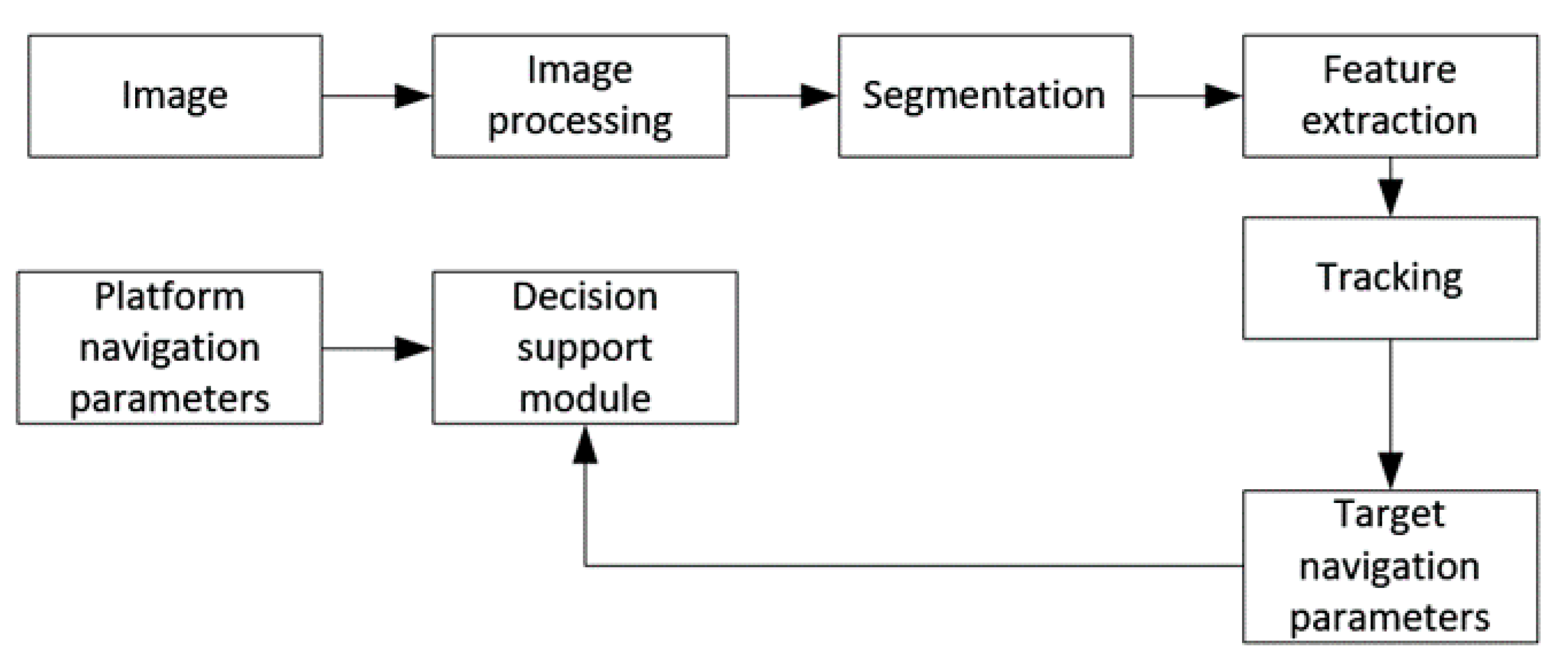
Acoustic imaging sensors are an alternative to these systems, among which the most popular solution for anti-collision is FLS. Figure 1 presents the process flow of an FLS.
All data used in the process of developing the appropriate decision originates from sensors mounted on the unmanned floating platform. The sonar image analysis is focused on the identification of objects in the head sector of the moving platform, which enables a rapid detection. The sonar image is then provided to the data processing system and is pre-processed by segmentation methods to locate the edges of the objects and set targets. The aim of the tracking block in the system is first the determination of centroids or characteristic points for approximating parameters and then full state vector estimation. In combination with defined anti-collision maneuvers, in the process of decision support, an anti-collision maneuver is made and collision with the object is avoided.
The group of acoustic devices that are used to obtain data for the anti-collision system can include mechanically scanned imaging sonars (MSIS) and multi-beam scanning sonars [11,12]. The quality of the imaging obtained, and hence the possibility of detecting a small object moving in the water, is influenced by the parameters of the acoustic beam that is generated, including the horizontal and vertical angle, as well as the frequency of the signal and refresh rate of the image. All devices work on a similar principle in that they generate an acoustic signal using the technique of sound propagation in water. The only difference between devices is the technique used to form the acoustic beam, which influences the measurement quality.
There have been interesting developments in sonar systems for underwater target tracking, with the development of systems that use the fusion of sonar with other techniques. For example in [13], the fusion of sensors in a hull mounted array is described, with a UKF used as the tracking technique. In [14], sonar information was enhanced using ultra short bearing line (USBL) data to increase the density of data and the object was tracked with a PF. In [15], another approach for fusion is given, in which information about effective sound speed velocity is included in the state vector. It is therefore not surprising that the fusion of various data is referred to in [3] as one of the main development fields in underwater target tracking.
Another development in sonar systems is 3D data processing and modeling. There are examples of the use of sonar data for the 3D modeling of targets in a water column, although without the verification of actual tracking [16,17]. An interesting approach to the tracking of bottom targets, including information about the height of the sensor, which means 3D tracking, is provided by [18].
These examples indicate that many applications involving underwater target tracking are being developed worldwide, however, they are based on various different methods.
2.2. Target Tracking in Sonar Anti-Collision
Basic models of the target tracking process have already been presented in Equations (1) and (2). Tracking, at this stage, means an estimation of an object’s movement parameters or more precisely an estimation of the state vector, based on updated measurements. Filtration methods are used in this process because the estimated state iteratively includes information about all previous states that are accumulated in the existing state. When the measurement is made, the state is updated taking into account the accuracy of the measurement and the estimated state. This accuracy is presented in the form of a covariance matrix, including a process noise matrix. The exact definition of the elements of these models varies among the different tracking algorithms. A numerical filter, typically a modification of the KF, is used in this process; however, the PF is becoming increasingly popular and in some cases neural tracking filters are used. In our research we propose to use the implementation of Kalman Filter, however the process noise analysis are useful also for other numerical solutions. Therefore a short literature review of tracking algorithms is provided in this section.
The review included in [3] provides a detailed description of numerical filters used for underwater target tracking, indicating that in linear conditions, a KF provides the optimal estimation. This situation is however relatively rare in real environments, therefore in real life applications sub-optimal algorithms are often used, including the EKF, UKF, and PF. The EKF is the nonlinear expansion of the classical KF. It adopts a Taylor series to linearize the nonlinear part and obtains a sub-optimal estimation. An example of the use of EKF in underwater target tracking can be found in [1,4,15,19]. An UKF approximates the nonlinear distribution using a set of discrete, weighted samples, called particles and makes an approximation of the posterior probability density function (PDF) of the state. The precision of the UKF can be compared to the second order EKF [3]. An example of the use of a UKF can be found in [4,9,13]. The PF on the other hand is an algorithm that performs a vector state estimation based on random sampling for approximating the posterior PDF in nonlinear or non-Gaussian problems. In such cases, the PF approximates the PDF directly from a set of random sampling points; therefore, it is claimed to provide more precise estimations than the EKF [3]. The usefulness of the PF for underwater target tracking was proven for example in [14,20]. Some other interesting modifications and adaptations of the KF are reported in the literature, and are mostly dedicated to specific applications, such as maneuvering target tracking or multiple-target tracking [19,21]. An interesting approach to underwater target tracking is also use of the neural networks, proposed for example in [22] as a modification of radar target tracking methods.
Specific algorithms have also been developed for tracking targets in underwater wireless sensor networks. One of the most popular is 3D underwater tracking (3DUT), proposed in [23]. The location of the target is determined within the network area using trilateration at the sink node. Various modifications of this algorithm have been proposed in the literature [3].
A large variety of tracking filters have been deployed to estimate the state vector of targets tracked under water. In each case the general assumptions are the same, although the model is slightly modified. This also applies to the model of process noise, as will be described further.
2.3. The KF Structure for Sonar Target Tracking
The KF structure is already well known because it has been widely used in tracking applications for a long time. The KF has superseded most approaches used in earlier algorithms, such as the α-β or α-β-γ filters. A review of its applications showed that the structure used for underwater target tracking is basically the same; however, the filters differ in their implementation in particular models and matrices. Therefore, for the clarity of the research process, we provide in this section our full implementation of Kalman Filter in the research system. It is based on the most popular approach [4] in which the process is modeled with the state equation in discrete time with Equation (3) and the measurement model is based on polar coordinates as given in Equation (6). Own implementation suited to FLS system, based on polar coordinates is proposed with expanded analysis of covariance matrix (Section 2.4).
where T is the sampling time; xk is the state vector defined as in Equation (4); Fk is the transition matrix and Wk is the process noise; which will be explained in the next subsection; and k is an indication of a step in time.
where (x, y) is the target position in Cartesian coordinates and (Vx, Vy) is the target speed along the coordinate system axis. The coordinate system may be different depending on the approach. The most widely used is the local coordinate system, with the starting point in the sensor head location and the axis determined by the sonar axis. However, it is also possible to transform all the information into an external, terrestrial coordinate system, such as the Universal Transverse Mercator (UTM). The transformation may be done at the beginning or the end of the process.
It is also possible, and quite common, for the vector state to be determined in three dimensional space and the equations are therefore expanded to the third dimension. However, in our study the aim was to work directly with sonar sensor measurements in a sonar two dimensional plane.
Other definitions of the state vector are also possible. An interesting approach is presented in [18], where the state vector is defined in polar rather than Cartesian coordinates. This requires other definitions of the transition matrix.
In the classical approach the transition matrix F is fixed all the time; however, in some cases (e.g., multi-model filters) it may change, and therefore an indication of the step time is required.
In each iteration of the KF algorithm, the prediction is made based on state Equation (3) and the prediction of state vector covariance has the form of:
where Pk+1/k is the covariance matrix of the next predicted state; Pk is the covariance matrix of the last estimate; and Qk is the process covariance matrix, which will be explained further.
In each iteration of the KF algorithm, the state vector is updated with the measurement. In the case of sonar, the general measurement model presented in Equation (2) is usually expanded in the form of Equation (6):
where θ is a bearing (relative) angle; d is the distance to the target being measured with sonar; and vk is white Gaussian additive noise, with a covariance matrix (7):
where σθ is the bearing measurement variance and σd is the distance measurement variance. Both are assumed to be independent, therefore the covariances are 0.
The innovation and its covariance is then calculated, as well as the final estimate together with its covariance. The KF equations are well known. One of the most important advantages of KF is that it not only estimates the value but also provides the covariance of the estimate, which allows the quality of the filtration process to be assessed.
The matrices presented in this subsection present the classical, linear KF approach. The modifications mentioned earlier, such as the EKF and UKF, which head towards nonlinearization and other adaptations require a modification of these matrices (mostly the transition matrix F) according to the assumed linearization model. A detailed description of this may be found in the literature and is beyond the scope of this paper.
2.4. Process Noise Models
One of the important elements of the filter used in the analysis is the modeling of process noise, which has a crucial impact on the performance of the KF during the estimation. Noise values that are too small may cause the filter to follow the estimates and ignore measurements, causing a so called lag error. Noise values that are too large will result in a noisy estimation if the estimates are followed strictly. Thus, the model of process noise should be adequately developed. Therefore in this subchapter we focus on process noise modelling in different papers and in the end we propose our approach suitable for these research.
Process noise is included in state Equation (3) as wk, denoting a zero mean Gaussian process with a known covariance matrix Q. The determination of the Q matrix should include all the factors that influence the process, which are not modeled directly in the equation. Depending on the elements of the Q matrix it may be required to multiply it by another factor to recalculate the influence on state vector elements. Taking this into account, the final form of the state transition equation is:
where G is called the transform matrix and wk ~ N(0,Qk). Thus, the crucial part for process noise modeling is the determination of the elements of the covariance matrix Q. Depending on the application, a discrete or continuous noise model can be used. In tracking applications, a discrete noise model is commonly used, and therefore the matrix elements are given directly. In other applications, the discretization of the model over time would be necessary.
In a discrete noise model, the elements of the process noise covariance matrix should represent the variations of state vector elements, which are not (or cannot be) modeled within the filter equations. In general, for a discrete noise model, the covariance matrix has the form of:
where σx, σy, σVx, and σVy are the standard deviations of x, y, Vx, and Vy, respectively. It is common practice to assume all the variables are independent. Then, the covariance matrix is simplified to a diagonal matrix diag(σx, σy, σVx, σVy).
The elements of the covariance matrix can directly indicate a disturbance in the vector state, but in many cases it is convenient to represent it in terms of an unknown acceleration affecting the target and therefore disturbing the process itself. The noise vector wk represents the random acceleration in both dimensions, and covariance and transform matrices then have the form indicated in Equations (10) and (11), assuming the independency of ax and ay.
Such an approach can be found in [3,4,24], and a similar idea is also presented in [13]. However, because the vector state model was modified by the coordinate transformation, the resulting system noise was given as the variation of the bearing. This acceleration based concept was also expanded in an interesting way in [19], in which an interacting multiple model (IMM) filter was constructed. A constant velocity model and constant acceleration model were incorporated in the IMM. In both models, the variation in the values of the covariance matrix represented unknown accelerations. In the constant acceleration model the values were smaller because part of the acceleration (known acceleration) was already included in the state model.
In [25], an example of the use of a KF in a UWSN was presented. The covariance matrix was proposed in its typical acceleration form; however, the state vector was defined in three dimensions, which caused the covariance matrix to be modified to a 3D plane (6 × 6 matrix). Although it is an example of non-FLS application, the tracking problem and filters follows the same principals. Therefore it is also worth of taking into account for analysis.
In [18], the approach was slightly different, with the state vector defined in polar coordinates. The authors proposed the creation of a covariance matrix that directly represented distance and bearing noise by taking into account the theoretical precision of navigation sensors.
In [15], the authors proposed the calculation of positional variance based on velocity and course variance, and thus the covariance matrix for a traditional model had the form of:
where σw is the standard deviation of the in-water speed component of the vessel uncertainty; σc is the standard deviation of current speed; and ωk is the vessel’s course at moment k. This interesting approach allows a closer investigation of the nature of process noise. In [15], an additional covariance matrix was proposed for an adaptive KF, including a sound velocity estimation but this was beyond the scope of this paper and there was no difference in the basic components.
An even more precise investigation of the covariance matrix elements was proposed in [26]. The approach was used for radar tracking and led to an interesting comparison of a numerical and neural filter in [27]. We propose to use a similar approach for underwater sonar target tracking and we will analyze it in detail in further part of the paper. The covariance matrix was proposed in the form of Equation (9), while the elements were thoroughly specified and the factors influencing the process were indicated according to the following equations:
where σVρ is the standard deviation of the relative velocity and σωρ is the standard deviation of the relative course; Vρ denotes the relative velocity; and ωρ denotes the relative course. Relative course and velocity means here the values representing the movement of the target in relation to sensor carrying vessel, unlike values calculated in relation to external (usually geographically based) coordinate system, called in navigation true course and true velocity. In practice, relative movement vector, representing relative course and velocity, is a geometrical sum of target true movement vector and own ship true movement vector.
In this approach all the variance and covariance values are calculated in relation to the relative course, the speed of the sensor carrying vessel and their variances. This wide concept of process noise is derived from the nature of the radar tracking process, in which the measurement environment is also an important factor affecting the measurement accuracy. It can sometimes be even more important than the sensor properties themselves.
Summing up this subsection, the most popular approach to the modeling of process noise in underwater target tracking is to assume that the noise is unknown accelerations, having an additive Gaussian distribution. The covariance values are usually arbitrarily selected based on the experience of the authors. Accelerations along both axes are usually assumed to be independent, which leads to a diagonal covariance matrix. However, in some applications, the nature of process noise is examined and the values of the covariance matrix are set based on navigational sensor errors and the influence of the environment. The present study therefore conducted a theoretical analysis of underwater target tracking process noise and an empirical verification of this analysis.
3. Materials and Methods
The goal of the study was to determine the elements of the process covariance matrix in numerical filters for the tracking of floating objects with FLS. The intention was to support a theoretical analysis with empirical research based on real data recorded with MSIS. It was assumed that the empirical research will improve our understanding of the sonar tracking process and will enable process noise to be more effectively determined in this application. The proper selection of process noise variance and an appropriate model should result in better tuning of the tracking filter to the particular problem, which can be understood as a compromise between tracking accuracy and noisy estimates.
A theoretical analysis was performed based on selected literature and performance standards for the equipment. The focus was on FLS applications and research; however, other techniques for underwater tracking (e.g., UWNS and sensor arrays) were also included as the nature of object movement underwater was the same.
The empirical analysis was based on post-processing of the sonar images, including feature selection and centroid extraction. A set of images was processed with analytical software, the targets were isolated and their relative positions were analyzed. For the positional components of process variance the changes in the target’s position were statistically estimated. For velocity components the changes in the movement of a sonar carrying platform were analyzed indicating the precision of the relative course and speed determination.
3.1. Research Equipment
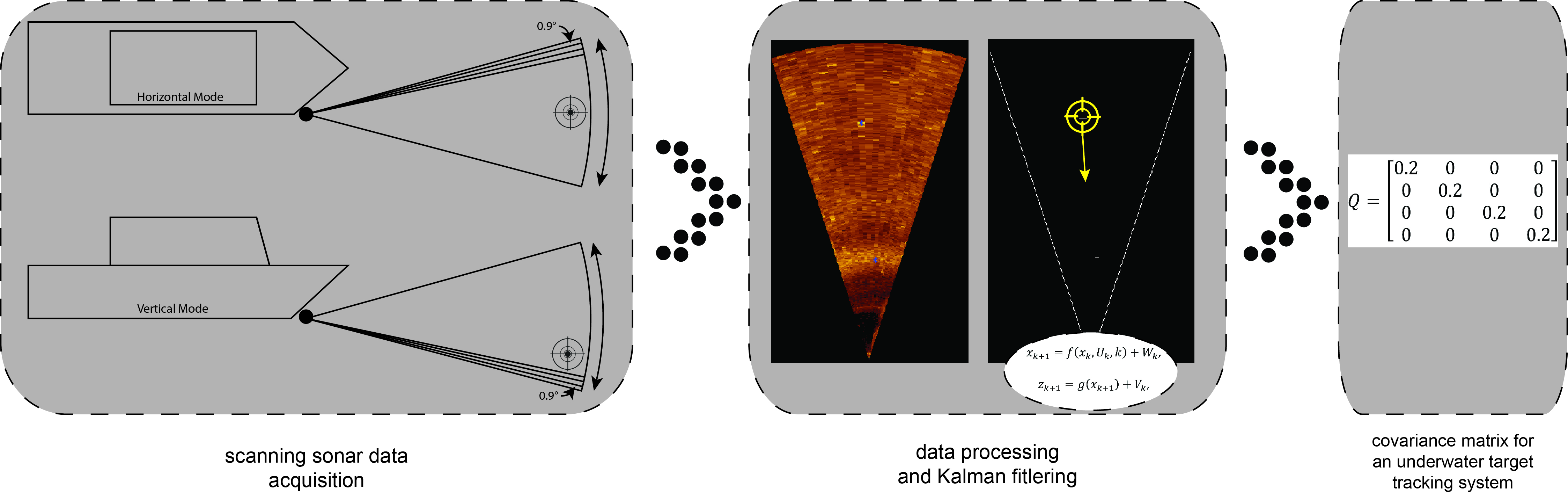
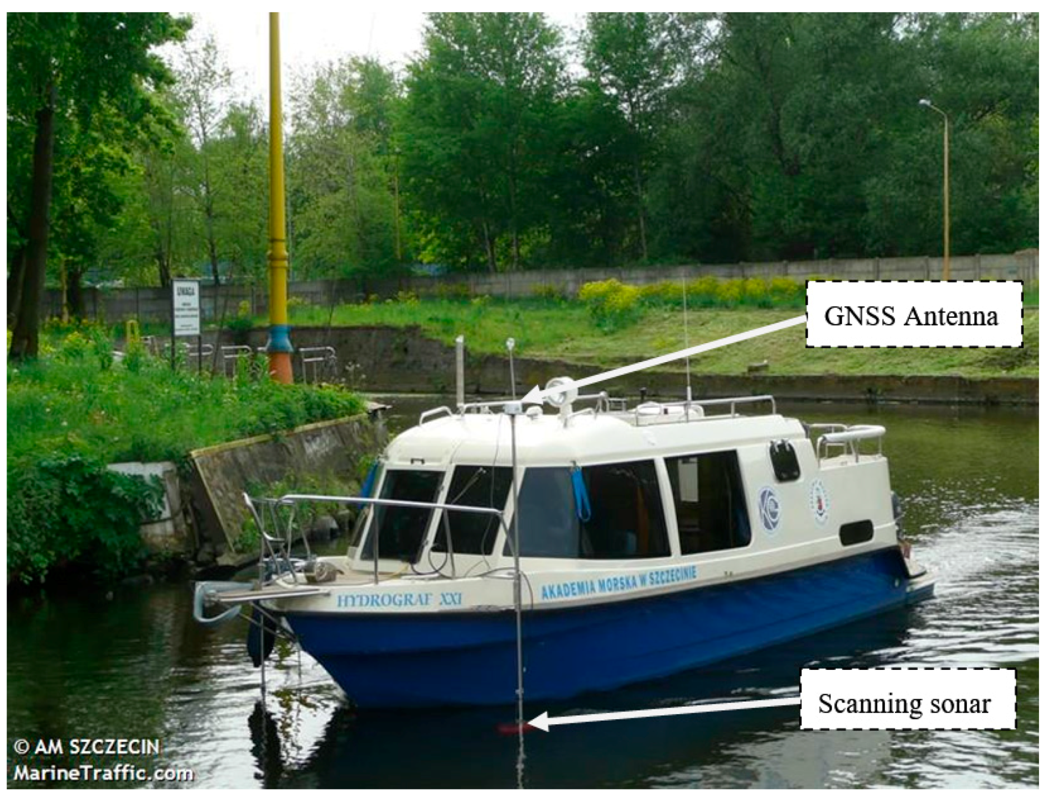
The measurement system used in this study simulated a system that could be installed on an unmanned floating platform. The main element of the system was an MSIS type sonar, mounted in two modes for horizontal and vertical data acquisition. The second element of the system was a Global Navigation Satellite Systems (GNSS) satellite positioning system. Both devices were installed on the research and hydrographic boat Hydrograf XXI (Figure 2). This provided an alternative to conducting research with the use of AUV. Although the measurement system was not able to simulate all of the actual conditions of a platform conducting measurement missions, for a tracking scenario it represented a suitable approach.
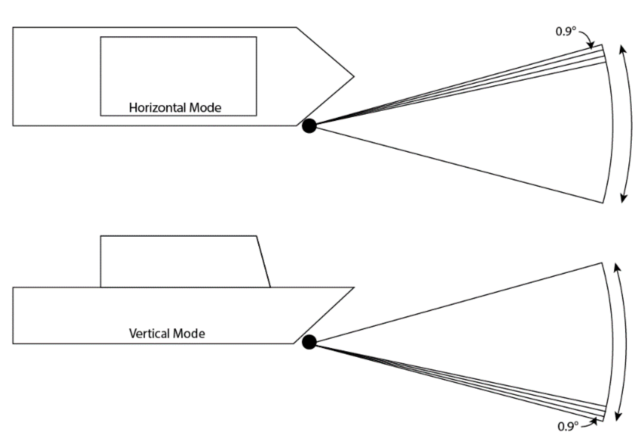
The MSIS used in the survey was the MS1000 model (Kongsberg ASA, Kongsberg, Norway). The MS1000 scanning sonar, with a frequency of 675 kHz, enables high resolution images to be obtained. It is designed especially for seabed inspection, searching for drowning victims, underwater structure inspection, and other applications where a high resolution and sharpness of the image has priority over other sonar parameters. It is also often used on ROV vehicles as an additional source of information about the underwater situation. Table 1 shows the most important parameters of this sonar. In this research particular attention should be laid in beam width. In typical installation, further referred as horizontal mode, 0,9° can be treated as bearing resolution and 30° as elevation resolution. In case of mounting in vertical mode, in which sonar head is scanning vertically, bearing resolution is 30° and elevation resolution is 0.9°.
A 5–l bottle connected to two buoys with a thin line was used as a target object floating in the water column. The weight of the object was sufficient for it to remain suspended freely in the water at a depth of approx. 1.5 m from the water surface. The object was not anchored and was therefore exposed to the current and wind.
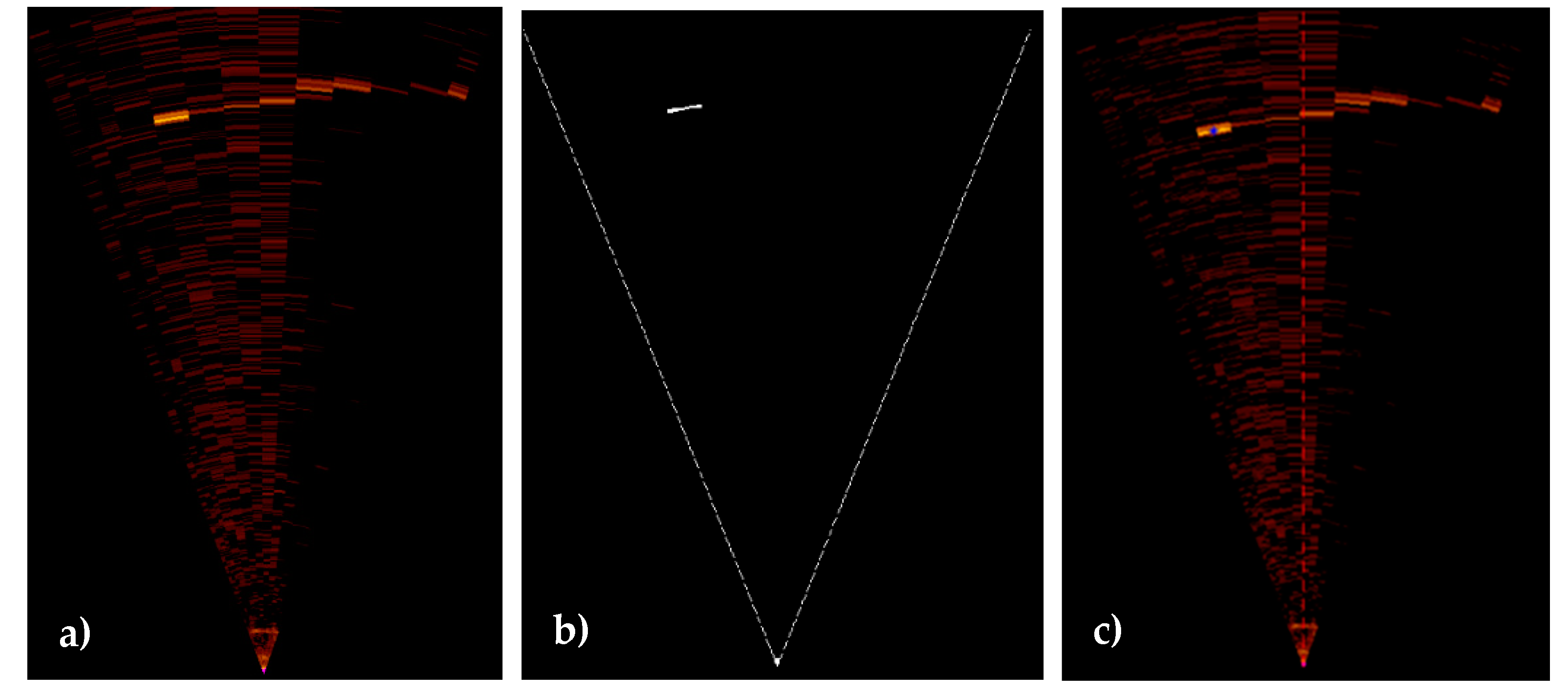
Matlab software was used to process the sonar images. The input data was in the form of 8-bit rasters, with a resolution of 1156 × 948 and 1428 × 952 pixels. Using raster image binarization methods, the object was separated into the background as black pixels and the object as white pixels. In the next stage, the centroids of the white pixel areas were calculated using the regionprops function. Figure 3 is an example from the binarization of data using the Otsu method [28]. From the left to right side of the figure, the input raster, binarization results in the form of differentiated pixels and with an overlaid centroid on the input data are presented. The centroids were also exported in the local coordinate system of the raster image.
3.2. Research Scenarios
The implementation of the planned research scenarios was focused on the simulation of a potential collision between a floating platform and a floating object. The research tasks were performed in the internal sea water basin of the Szczecin harbor (Odra River). The selected area was surrounded by harbor quays, where the influence of external parameters was conducive to the implementation of the planned tasks. Two main research tests were conducted, focusing on the possibility of detecting an object by sonar configured in the horizontal and vertical operational modes (Figure 4). The Global Navigation Satellite System (GNSS) satellite positioning system was used in one case and GNSS real-time kinematic (RTK) positioning was used in the other.
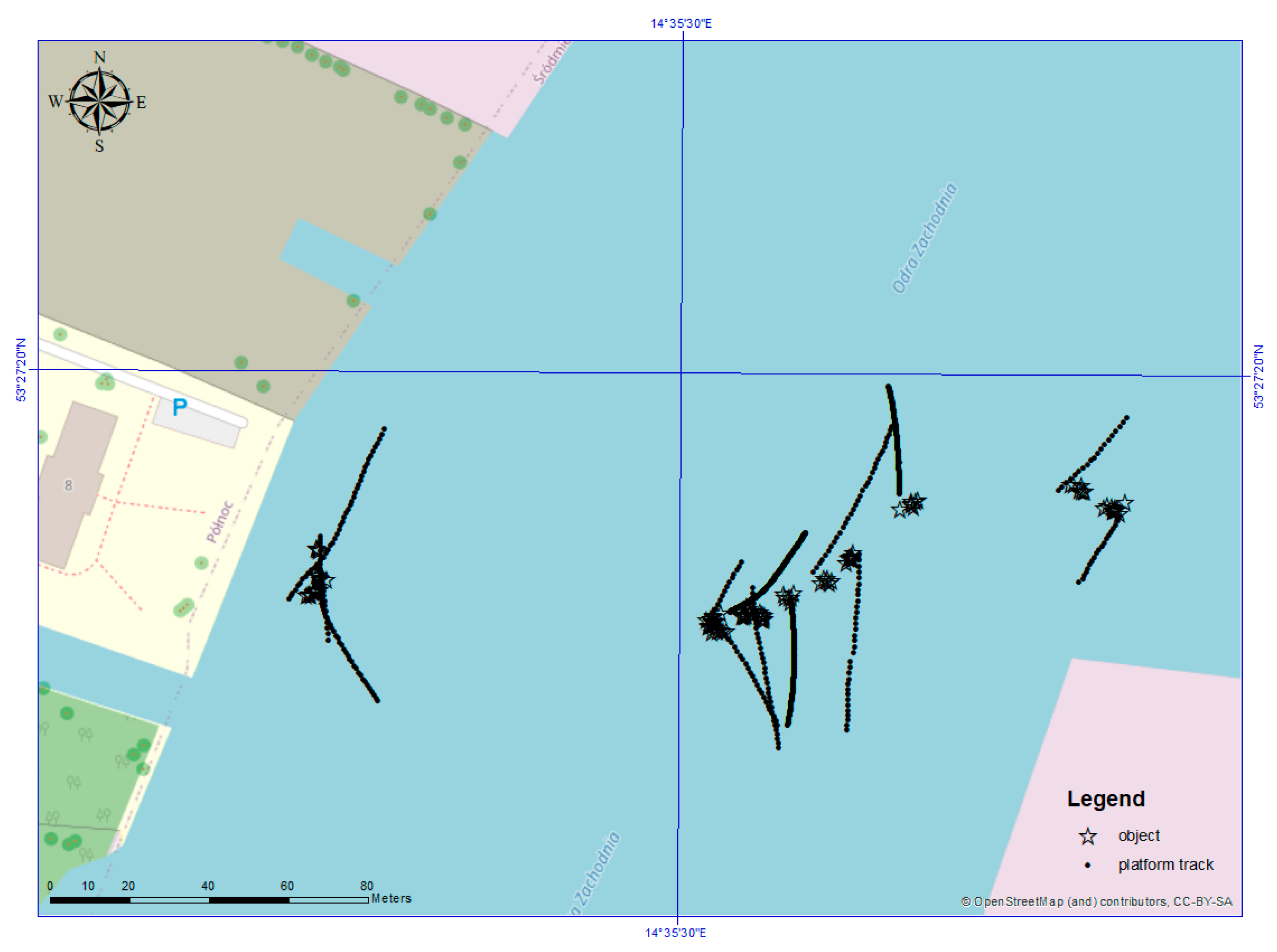
The course of the vessel was set to ensure that the target object was kept within range of the sonar. The course ran directly to the object, which simulated a collision course, and at the last moment the course was changed to avoid real contact with the object. The research scenarios are shown on the map in Figure 5.
The sonar data were recorded by the MS1000 sonar software. The software provides data acquisition, changes in sonar parameters, such as the range, sector, scanning speed, gain, and time-varied-gain (TVG) settings, as well as enabling the playback of recordings, with the ability to measure the dimensions and position of a target object, and to export data to raster files. The GNSS satellite positioning system and the RTK system, with real-time corrections, were connected to the computer with the above-mentioned software. This allowed the navigation data of the platform to be registered.
During the data logging process, a number of situations were registered in which the object was detected within the approaching course. From among the data, seven of these situations were selected for vertical scanning and three for horizontal scanning. It should be noted that in both cases the data did not originate from a single configuration of basic sonar operating parameters. The parameters that were changed were the sonar operating range, scanning head speed, and sector settings. Table 2 shows the registered configurations for each scenario. The final column shows the number of images that contained the detected object.
3.3. Data Evaluation
Data gathered in the research were processed and evaluated to determine the processes influencing data variance. The main indicators of variance were statistically obtained values of the accuracy and precision of the object and sonar position, as well as the movement parameters of the platform carrying the sonar, which means the values included in the covariance matrix presented in Equation (9) were:
- σx2—variance in the x direction (easting);
- σy2—variance in the y direction (northing);
- σVx2—variance of speed in the x direction;
- σVy2—variance of the related speed in the y direction.
For these values, the mean and standard deviation were used for comparison.
In the theoretical analysis, the values used in the literature for variance were presented and analyzed, with mean values and standard deviations calculated. To enable a comparison, the values were calculated for the assumed fixed interval (1 s) and if necessary transformed. In most previous studies, process noise was modeled as random accelerations; thus, transformations were performed to represent positional and velocity variances. Additionally, based on the device’s performance, an analysis was conducted of the theoretical errors of the determination of the relative course and speed. The influence of currents was also considered.
In the empirical analysis, the actual measured values and theoretically modeled values were compared. In the analysis of the course and speed of the platform, the theoretical track was modeled with a polynomial regression and any deviations were calculated. The descriptive statistics (average and standard deviation) of all measurements for the horizontal and vertical scenarios were calculated. Two different analyses were performed with regard to the object’s position. First, the deviation from the average position for each measurement was determined and descriptive statistics were calculated (excluding rough errors). The actual position of the object was recorded on the sonar screen by an experienced A-category hydrographer and was thus referred to as the expert position. This part of the research included an assessment of the variation in the object’s position due to environmental conditions.
In the second analysis, the differences between the expert position and centroids was determined. The aim was to include the centroid calculation error as part of the process noise. Such an approach should allow the extraction process itself to be included in system equations. The centroids themselves were calculated as the result of a feature extraction process, which included the binarization of the image and the determination of the coordinates of the center of gravity at the position of the object in the image. In the first stage of the input image binarization, three thresholds, the Otsu, local threshold, and im2bw [29] methods, were used to verify the correctness of the operation. With an appropriate binarization, the echo from the object could be distinguished from the image. Then, for such a simplified image, the coordinates of the centroids of the object were calculated using the regionprops function. The descriptive statistics, that is, average and standard deviation, were used to finally obtain the variance.
4. Results
The research conducted in this study included a theoretical analysis, measurements according to described scenarios, and data post processing. This generated the results presented in this section. The results are presented in two sections relating to the theoretical and empirical parts of the research, following a complex analysis of the issues undertaken.
4.1. Theoretical Analyses
The theoretical research was conducted in two stages. In the first stage, applications and solutions described in selected papers were analyzed. The results of this analysis are presented in Table 3. The table includes recalculated values (with the assumption of a 1 s time stamp) of the variances used in various approaches. The type of solution and variance values are followed by a list of variances. The data include all of the reviewed papers in which exact values were given. In other papers, numerical data were not provided. The number of samples was not very large, but a reasonable assessment of the values used could be attained because the deviation was relatively small.
The review presented in Table 3 indicates that the values of covariance matrix elements were small but non-zero, as stated in [24]. The standard deviation was reasonably small, indicating the consistency of the data. It was interesting that if taking into account only FLS applications, the actual values and standard deviations were smaller. Because this study focused on FLS, additional papers should be reviewed to provide reliable values for TASAs and UWSNs.
The theoretical analysis also allowed the variances due to environmental conditions and measurement errors of the navigational equipment to be determined. The state transition model should be complementary to the measurement model, providing a complex and reliable model to fit the specific tracking application. The key issues influencing noise in the state and measurement models were:
- environmental issues affecting the movement of the target in the water, for example, positional variations due to current, waves, and drift;
- environmental issues affecting the carrying platform, for example, position, course, and speed variations;
- errors in the navigational instruments on the carrying platform, for example, position, course, and speed variations;
- errors of sonar measurements, for example, target position variation;
- feature extraction algorithm errors, for example, target position variation.
It was proposed in this study to only model sensor errors in the measurement model, so providing producer accuracy values for the measurement covariance matrix (Equation (7)). Thus, the process noise model has to include all of the other issues. Platform position variance is expected to be filtered out by positional filters included in positional device. Environmental issues can be modeled by two factors. First, by the general drift added to the target position and second, by course and speed noises added to the ship data. However, both should be included as relative values. Such an approach would ease the formulation of a covariance matrix because course and speed variances will be modeled only once. Taking into account the assumption of x/y independency, the covariance matrix will be diagonal and the variances could be modeled as follows:
where σVxc2 and σVyc2 are the variances of the x and y components of the current speed and the other elements were defined in Section 2.4. The feature extraction error variances are represented by σxe2 and σye2. It is assumed that these values should not exceed 0.15 m, which is represented by 4–8 pixels (depending on the range). If the x/y independence assumption is not valid the covariance matrix should take into account Equations (13)–(20).
Current variance is strongly dependent on the geographical area. It can be assumed that in closed calm waters (e.g., lakes) the variance should not exceed 0.1 m/s, but in rivers the values can be up to 2–3 m/s. In such cases it might be reasonable to include the river current as a known input, and the remaining process noise would be small. Relative speed and course values can be obtained based on the accuracy of course and speed measurements affected by the additional noise. In [30], it was shown that the typical accuracy of course values determined by gyrocompass devices should not exceed 1.5°. Taking this into account and assuming additional movement of the target we proposed the accuracy of the relative speed and course to be 0.4 m/s and 2.5° (in terms of the standard deviation), which would lead to Vx and Vy variances of up to 0.25 m/s in calm waters (assuming a current velocity = 0.3 m/s). These values are higher than those calculated in Table 3, and therefore an empirical verification is required.
4.2. Empirical Research
The empirical research was conducted in three stages. The first two were used to determine positional variations and the final stage provided the velocity variance. It was assumed that velocity variance can be modeled directly from the platform’s track deviation analysis and that positional variance is the sum of two factors according to Equation (21).
4.2.1. Positional Deviation of the Object from the Mean Value
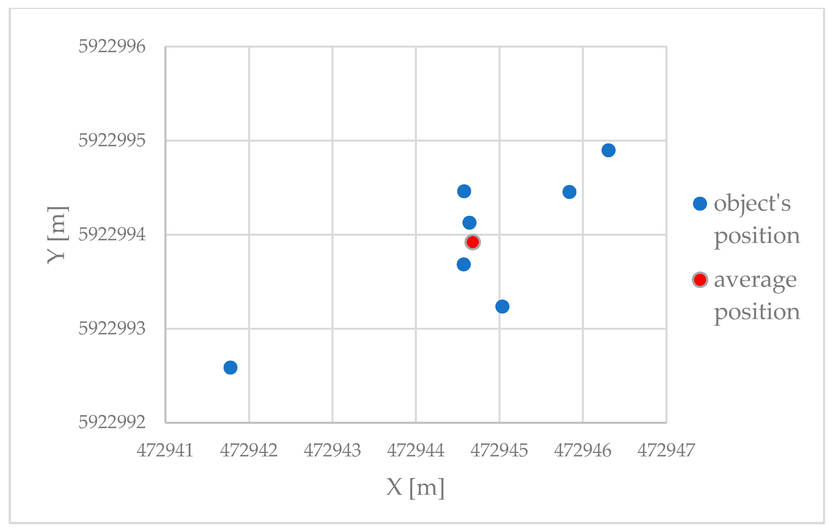
The geographical position was obtained by an expert using the sonar software during the data processing phase. Initially, the data had a World Geodetic System (WGS84) coordinate system. The position in φ and λ data was projected into the UTM coordinate system. Table 4 presents the deviation of the position from the mean value in the horizontal and vertical scenarios. The values are given independently for the x and y axes. Figure 6 shows a typical distribution of points in relation to the average position.
Table 4 shows the statistical differences between the horizontal and average coordinates. The standard deviations between the horizontal and vertical scenarios were similar but were slightly higher in the vertical scenario. The vertical alignment of the sensor is most often used to determine the position of an object in the vertical axis. When scanning in a wide angle, it becomes difficult to estimate the exact position of an object in the horizontal plane. This is especially the case at the ends of the measuring range, where due to the width of the scanning sector the error in determining the position is the greatest.
4.2.2. Deviations between Centroids and the Expert Position
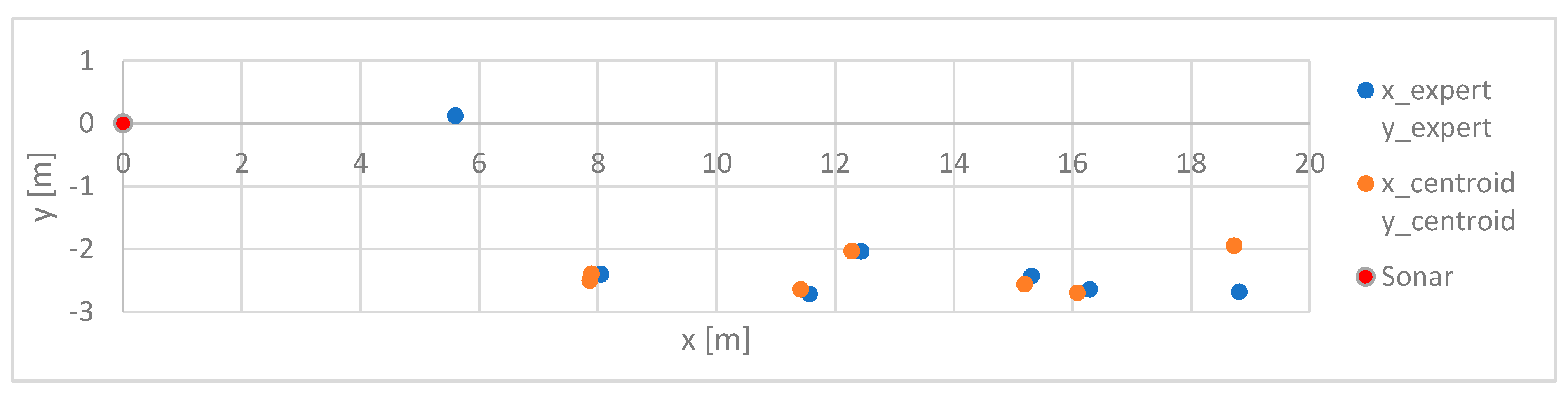
In this comparison, two data sources were used to establish the differences. The first was the position determined by an expert from a manual detection of an object’s position using the sonar software. The second position was obtained from automatic raster image processing together with centroid coordinates. Figure 7 shows the distribution of the points indicated by the expert in relation to the automatically determined centroid.
In this analysis, the coordinates were calculated in the local system related to sensor position and orientation. It can be seen that centroids mostly follows expert recommendations, however it may happen that the differences are big. The position indicated by the expert is a subjective position. Sonar images often display false echoes, which can influence the choice. The floating object itself can generate up to three echoes: from the object, the line and the buoy, which may also affect indications.
Table 5 provides the descriptive statistics regarding the difference in horizontal coordinates determined by the expert and the centroids from the image processing method. These were calculated as a result of a subtraction of centroid coordinate (orange dots on Figure 7) from expert coordinate (blue dots on Figure 7). The results confirmed the accuracy obtained using the centroid and identification method operated by the expert. The largest deviations were noted near the sensor. This may have been caused by the platform turning to avoid contact with the object, resulting in the echo being blurred in the sonar image. This made it difficult to determine the exact position of the object.
4.2.3. The Track Deviation of the Platform
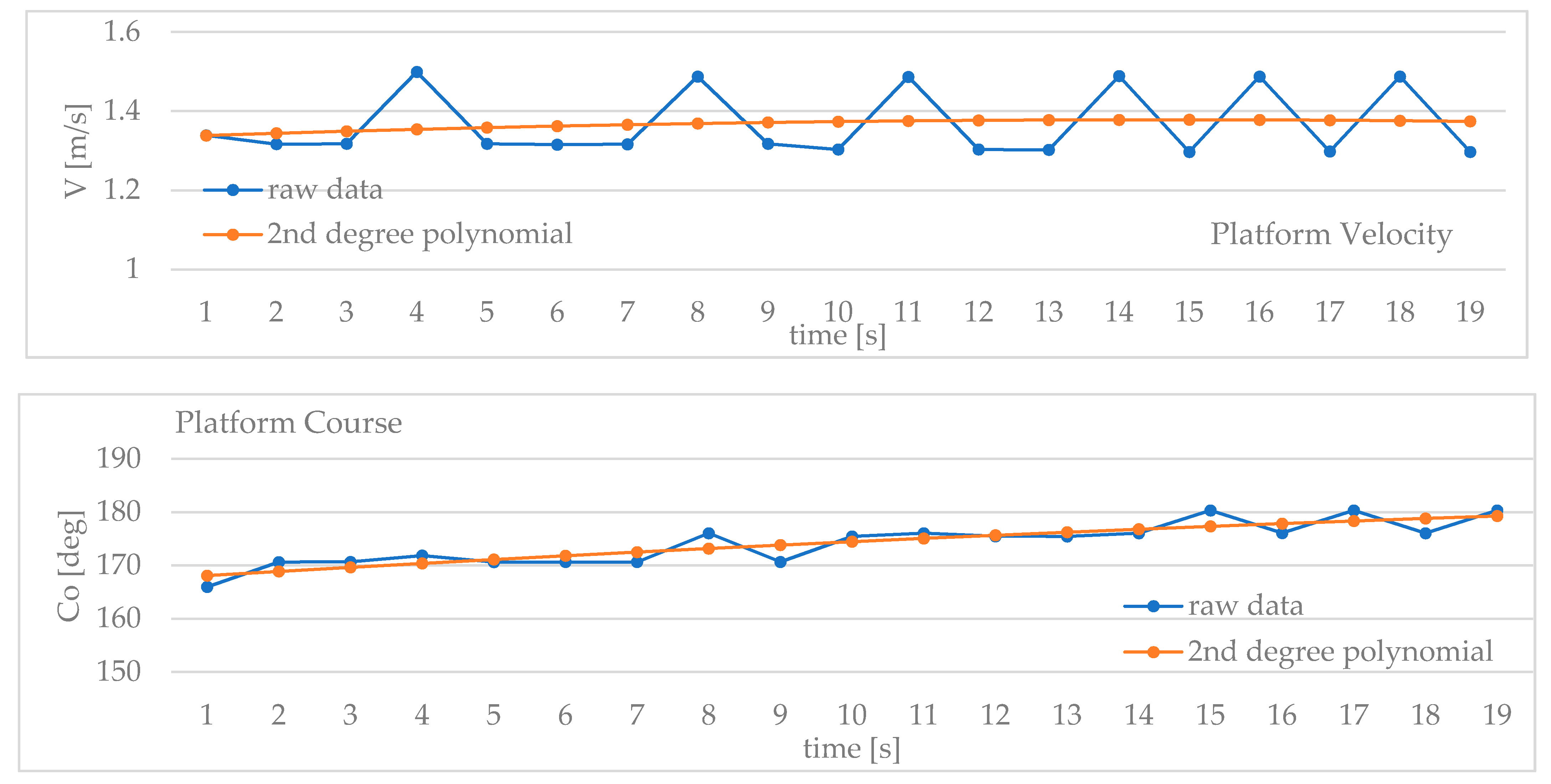
Large inaccuracies in the position and time received from the sonar’s native files indicated the need to determine the noise of the movement information acquired from the floating platform. The input data was recorded in NMEA 0183 format (National Marine Electronics Association). After initial analysis, it was decided to create a second degree polynomial to smooth the acquired course and speed data. In the next step, the difference between the input data and the polynomial was determined. Figure 8 shows a comparison of the raw data regarding velocity and the course of the platform, with the data determined on the basis of the second degree polynomial.
The statistical results for this scenario are presented in Table 6. The table includes differences of course (dco) and velocity (dv) between values from raw data and 2nd degree polynomial estimation as calculated in these scenarios. In case of raw course and velocity, the values were derived directly from two consecutive positions without any filtration. In case of 2nd degree polynomial, course and velocity values were derived directly from two consecutive estimated positions. The latter were treated as reference values for obtaining error of the former and the values presented in Table 6 relates to differences between them. The error values for velocity were very small, but the heading results had larger errors. In this study, the movement of a floating platform was based on only one positioning system on the basis of which all possible movement parameters were calculated. It was predicted that positioning values supported by systems guaranteeing better accuracy for the course, that is, a gyrocompass or an inertial navigation system (INS), and a log device for the speed would reduce the error results obtained. Because the target was meant to be stationary, the values in the table were treated as relative.
5. Discussion
The results indicated that there are quite important differences in the common approaches used to arbitrarily select covariance matrix values, the analytical approach, and empirical verification. In Table 7 a summary of the variance values obtained in this study is presented. In empirical research the values were recalculated to present the variations of position and velocity. The positional variance was the sum of an object’s positional deviation variance and the centroid’s deviation variance. For velocity variances (σVx and σVy), Equations (13) and (14) were used and the course and speed variance was calculated based on speed and course deviation presented in Table 6 according to Equations (24) and (25). This approach allowed representation of deviations at 95% confidence level.
where and are mean values for course and speed deviation taken from Table 6, while and are standard deviations for course and speed deviation taken from Table 6. These values have been recalculated to radians to represent linear values. Speed value included in Equations (13) and (14) as related velocity was set to 4 knots, as this is typically maximum speed at which the hydrographic soundings are being made. Values of sinus and cosinus functions used in Equations (13) and (14) were set in these calculations to 1 as it allowed to calculate maximum possible value.
The analysis of the results presented in Table 7 showed that the values determined both analytically and empirically were significantly larger than those proposed in most publications, especially for empirical determination of position variance. In case of position, one of the reasons for this might be the use of extraction error in our proposed system. For velocity, one of the reasons might be the use of a current analysis in our model. These findings show that the process covariance matrix and process noise model generally have to be treated as part of a complex tracking model. Some issues, such as the variances of the current or the platform’s movement may be included in other equations of the model. This would probably result in reducing noise values, but would also result in increasing model complexity, which is unwanted in this particular research. Further improvement of model for practical applications is possible, however does not fall into the scope of this paper.
It should be noticed here that values in covariance matrix, understood as a kind of hyper-parameters of filter, may serve in practical applications as tuning parameters. Final values of them are often found and set to optimize FLS results in the particular implementation. Therefore quite often they do not look for physical tuning justification. This approach seems to be reasonable as the tracking algorithm is a simplified model of physical random process. However, taking into account that these parameters can influence the performance of the filter, they have to be set with caution. Therefore, even if the values of hyper-parameters are to be set as a result of optimization process the knowledge given in the paper may be useful for proposing the optimization process and its initial values.
The results also showed that, in general, values achieved in the empirical research are bigger than the values derived from an analytical approach. There were two likely reasons for this: (1) environmental conditions found at the scene, where the current in the river was bigger than assumed in the theoretical approach; and (2) the positional systems used, which were of navigational and not hydrographical class. Significantly larger values were obtained for vertical scenarios. The reason for this was the sensor construction, with the vertical beam angle being much larger than in the horizontal scenario. For horizontal and vertical uses of the sonar, different values should be used.
From the analysis of previous research it was apparent that most of the authors made the assumption of the independency of variables, which makes the covariance matrix much simpler (diagonal). This assumption seems to be a reasonable simplification. Changing Vx or x does not mean an automatic change of Vy and y. On the other hand, these values are bounded with course and speed values (especially in the case of relative values). This may also be suggested by significantly smaller values of easting variance, compared to northing variance. It also seems to be reasonable to independently analyze positions and velocities as other factors may affect them in the tracking process.
This analysis led to a final proposition of a covariance matrix for an underwater target tracking system, presented as a model in the form of Equation (26), which is a classical horizontal sonar position:
6. Conclusions
This paper presented the results of a complex noise modeling study for acoustic underwater target tracking, with a focus on FLS. Three kinds of analysis were performed; an analysis based on references, followed by a theoretical analysis and empirical verification. In general, the noise could be modeled as white additive noise, representing unknown accelerations. It was, however, shown that the noise (elements of a covariance matrix) can also be arbitrarily defined and does not have to follow the definition of an acceleration. The analytical approach focused more on the reasons for position and velocity deviations, while the empirical research measured these two values and not the accelerations. The analysis of publications showed that very small values of noise variance were used. This indicates a relatively high belief in the process contingency. Such a concept has the risk of underestimating the influence of environmental conditions.
In the theoretical analysis, the results achieved were surprisingly large. The influence of current and navigational instrument errors were included and were assumed to have led to the high values. The values were 10 times larger than the values for FLS reported in the literature. Using values that are too large might result in an overestimation of measurement accuracy in the filter estimate, leading to inaccurate values. Therefore the covariance values should be proposed carefully. It should be noted that the empirical research generally confirmed the values proposed in the analytical approach. However in case of speed variation empirical values are smaller and in case of position variances they are mostly larger (except for σy for horizontal scenarios).
The most probable reason for large position variances is including the feature extraction error in the calculation and observation. The process of feature extraction is usually done before tracking itself. Publications usually focus on the tracking of already extracted features and therefore they do not have to include this error. Here, we performed the analysis of entire process. Feature extraction error was analytically estimated as 0.15, however empirical research shows that this estimation was too small.
In the case of velocity variances estimation, the most probable explanation for values larger than those presented in the literature is the inclusion of water current in our analysis. The scenarios took place in the river and therefore we decided to include it in the system, which is usually not the case. For analytical research 0.3 m/s was used; however, in the case of empirical research smaller values were achieved.
In conclusion, the values of covariance matrix elements should be set as relatively small, but not too small. It was confirmed that commonly used white noise assumption for covariance matrix elements is a proper approach. However, the values that were significantly less than the 0.1 met in the literature seem to underestimate real noise of the tracking process itself. If such values are the results of filter tuning in simulation conditions, it is advised to verify them in empirical research. Obtaining exact values used in the filter depends strongly on the modeling of the entire process and the measurements. The model can be different in each application, which may result in other values of covariance matrix elements. Based on this research, it can be said that, in the approach proposed here, with extraction error and river current included, the white noise variance for position should have a value between 0.1 and 0.3, while for velocity it should be from 0.15 to 0.25. It is also advised to use a diagonal covariance matrix; however, further studies are planned to empirically verify the assumption of the independency of variables.
Author Contributions
Conceptualization, W.K. and G.Z.; methodology, W.K.; literature review, G.Z. and W.K.; acquisition and analysis of data, G.Z., W.K.; interpretation of results, W.K. and G.Z.; writing—original draft preparation, G.Z.; writing—review and editing, W.K. All authors have read and agreed to the published version of the manuscript.
Funding
This research was conducted under grant no. 1/S/KG/21, financed from a subsidy of the Ministry of Science and Higher Education for statutory activities in the Maritime University of Szczecin.
Data Availability Statement
The data presented in this study are available on request from the corresponding author. The data are not publicly available due to privacy issues.
Conflicts of Interest
The authors declare that they have no conflict of interest regarding the publication of this paper.
References
- Modalavalasa, N.; Rao, G.S.; Prasad, K.S. An Efficient Implementation of Tracking Using Kalman Filter for Underwater Robot Application. Int. J. Comput. Sci. Eng. Inf. Technol. 2012, 2. [Google Scholar] [CrossRef]
- Stateczny, A.; Błaszczak-Bąk, W.; Sobieraj-Żłobińska, A.; Motyl, W.; Wisniewska, M. Methodology for Processing of 3D Multibeam Sonar Big Data for Comparative Navigation. Remote Sens. 2019, 11, 2245. [Google Scholar] [CrossRef] [Green Version]
- Luo, J.; Han, Y.; Fan, L. Underwater Acoustic Target Tracking: A Review. Sensors 2018, 18, 112. [Google Scholar] [CrossRef] [PubMed] [Green Version]
- Peyvandi, H.; Farrokhrooz, M.; Roufarshbaf, H.; Park, S.J. SONAR systems and underwater signal processing: Classic and modern approaches. SONAR Syst. 2011, 173–206. [Google Scholar] [CrossRef] [Green Version]
- Stateczny, A.; Kazimierski, W.; Gronska-Sledz, D.; Motyl, W. The Empirical Application of Automotive 3D Radar Sensor for Target Detection for an Autonomous Surface Vehicle’s Navigation. Remote Sens. 2019, 11, 1156. [Google Scholar] [CrossRef] [Green Version]
- Li, J.; Zhang, J.; Zhang, H.; Yan, Z. A Predictive Guidance Obstacle Avoidance Algorithm for AUV in Unknown Environments. Sensors 2019, 19, 2862. [Google Scholar] [CrossRef] [PubMed] [Green Version]
- Stateczny, A.; Gronska-Sledz, D.; Motyl, W. Precise Bathymetry as a Step Towards Producing Bathymetric Electronic Navigational Charts for Comparative (Terrain Reference) Navigation. J. Navig. 2019. [Google Scholar] [CrossRef]
- Wlodarczyk-Sielicka, M.; Stateczny, A. Selection of SOM Parameters for the Needs of Clusterisation of Data Obtained by Interferometric Methods. In Proceedings of the 16th International Radar Symposium (IRS), International Radar Symposium Proceedings, Dresden, Germany, 24–26 June 2015; Rohling, H., Ed.; 2015; pp. 1129–1134. [Google Scholar]
- Kumar, D.R.; Rao, S.K.; Raju, K.P. Integrated Unscented Kalman filter for underwater passive target tracking with towed array measurements. Optik-Int. J. Light Electron Optics 2016, 127, 2840–2847. [Google Scholar] [CrossRef]
- Felemban, E.; Shaikh, F.K.; Qureshi, U.M.; Sheikh, A.A.; Qaisar, S.B. Underwater sensor network applications: A comprehensive survey. Int. J. Distrib. Sens. Netw. 2015, 11, 896832. [Google Scholar] [CrossRef] [Green Version]
- Wawrzyniak, N.; Stateczny, A. MSIS Image Positioning in Port Areas with the Aid of Comparative Navigation Methods. Pol. Marit. Res. 2017, 24, 32–41. [Google Scholar] [CrossRef] [Green Version]
- Wawrzyniak, N.; Włodarczyk-Sielicka, M.; Stateczny, A. MSIS sonar image segmentation method based on underwater viewshed analysis and high-density seabed model. In Proceedings of the 18th International Radar Symposium (IRS), Prague, Czech Republic, 28–30 June 2017; pp. 1–9. [Google Scholar]
- Rao, S.K.; Murthy, K.L.; Rajeswari, K.R. Data fusion for underwater target tracking. IET Radar Sonar Navig. 2010, 4, 576–585. [Google Scholar] [CrossRef]
- Mandić, F.; Rendulić, I.; Mišković, N.; Nađ, Đ. Underwater object tracking using sonar and USBL measurements. J. Sens. 2016, 2016. [Google Scholar] [CrossRef] [Green Version]
- Deng, Z.-C.; Yu, X.; Qin, H.-D.; Zhu, Z.-B. Adaptive Kalman Filter-Based Single-Beacon Underwater Tracking with Unknown Effective Sound Velocity. Sensors 2018, 18, 4339. [Google Scholar] [CrossRef] [PubMed] [Green Version]
- Kraeutner, P.; Brumley, B.; Guo, H.; Giesemann, J. Rethinking forward-looking sonar for AUV’s: Combining horizontal beamforming with vertical angle-of-arrival estimation. In Proceedings of the IEEE OCEANS 2007, Vancouver, BC, Canada, 29 September–4 October 2007; pp. 1–7. [Google Scholar] [CrossRef]
- Karabchevsky, S.; Braginsky, B.; Guterman, H. AUV real-time acoustic vertical plane obstacle detection and avoidance. In Proceedings of the 2012 IEEE/OES Autonomous Underwater Vehicles (AUV), Southampton, UK, 24–27 September 2012; pp. 1–6. [Google Scholar]
- Quidu, I.; Bertholom, A.; Dupas, Y. Ground obstacle tracking on forward looking sonar images. In Proceedings of the 10th European Conference on Underwater Acoustics. (ECUA’10), Istanbul, Turkey, 5–9 July 2010. [Google Scholar]
- Li, W.; Li, Y.; Ren, S.; Feng, X. Tracking an underwater maneuvering target using an adaptive Kalman filter. In Proceedings of the 2013 IEEE International Conference of IEEE Region 10 (TENCON 2013), Xi’an, China, 22–25 October 2013; pp. 1–4. [Google Scholar]
- Clark, D.E.; Bell, J.; de Saint-Pern, Y.; Petillot, Y. PHD filter multi-target tracking in 3D sonar. In Proceedings of the IEEE/Europe Oceans 2005, Brest, France, 20–23 June 2005; Volume 1, pp. 265–270. [Google Scholar]
- Son, H.S.; Park, J.B.; Joo, Y.H. The study on tracking algorithm for the underwater target: Applying to noise limited bi-static sonar model. In Proceedings of the 2013 9th Asian Control Conference (ASCC), Istanbul, Turkey, 23–26 June 2013; pp. 1–6. [Google Scholar] [CrossRef]
- Kazimierski, W.; Zaniewicz, G. Analysis of the possibility of using radar tracking method based on GRNN for processing sonar spatial data. In Rough Sets and Intelligent Systems Paradigms; Springer: Cham, Switzerland, 2014; pp. 319–326. [Google Scholar]
- Isbitiren, G.; Akan, O.B. Three-dimensional underwater target tracking with acoustic sensor networks. IEEE Trans. Veh. Technol. 2011, 60, 3897–3906. [Google Scholar] [CrossRef]
- Karoui, I.; Quidu, I.; Legris, M. Automatic sea-surface obstacle detection and tracking in forward-looking sonar image sequences. IEEE Trans. Geosci. Remote Sens. 2015, 53, 4661–4669. [Google Scholar] [CrossRef]
- Poostpasand, M.; Javidan, R. An adaptive target tracking method for 3D underwater wireless sensor networks. Wirel. Netw. 2018, 24, 2797–2810. [Google Scholar] [CrossRef]
- Stateczny, A. (Ed.) Radar Navigation; Scientific Society of Gdansk: Gdansk, Poland, 2011. (In Polish) [Google Scholar]
- Stateczny, A. Neural manoeuvre detection of the tracked target in ARPA systems. IFAC Proc. Vol. 2001, 34, 209–214. [Google Scholar] [CrossRef]
- Otsu, N. A threshold selection method from gray-level histograms. IEEE Trans. Syst. Man Cybern. 1979, 9, 62–66. [Google Scholar] [CrossRef] [Green Version]
- Solomon, C.; Breckon, T. Fundamentals of Digital Image Processing: A Practical Approach with Examples in Matlab; John Wiley & Sons: Hoboken, NJ, USA, 2011. [Google Scholar]
- Specht, M.; Specht, C.; Lasota, H.; Cywiński, P. Assessment of the Steering Precision of a Hydrographic Unmanned Surface Vessel (USV) along Sounding Profiles Using a Low-Cost Multi-Global Navigation Satellite System (GNSS) Receiver Supported Autopilot. Sensors 2019, 19, 3939. [Google Scholar] [CrossRef] [PubMed] [Green Version]
Figure 1.
The general signal flow in a system based on forward looking sonar.

Figure 2.
The research and hydrographic boat Hydrograf XXI.

Figure 3.
The sequence of image processing steps to obtain a centroid: (a) a vertical measurement input image, (b) a binarized image, and (c) an input image with a defined centroid.
Figure 3.
The sequence of image processing steps to obtain a centroid: (a) a vertical measurement input image, (b) a binarized image, and (c) an input image with a defined centroid.

Figure 4.
Measurement scheme for the horizontal (top) and vertical (bottom) scenarios.

Figure 5.
Overview of the track of the floating platform and the target object.

Figure 6.
Example of the object’s position and the average position for VER_1 (UTM coordinates).

Figure 7.
Example of the deviation between centroids and expert position in the scanning sonar position for VER_1 (local sensor coordinate system).
Figure 7.
Example of the deviation between centroids and expert position in the scanning sonar position for VER_1 (local sensor coordinate system).

Figure 8.
Example of the velocity and course platform for VER_1.


Table 1.
Specification of the scanning sonar used in the research.
| Model | Kongsberg MS1000 |
|---|---|
| Frequency | 675 kHz |
| Beam width | 0.9° × 30° |
| Range | typical 0.5–100 m obtainable 150 m |
| Along track resolution | ≥19 mm (at a sound speed of 1500 m/s, transmit pulse length 25 μs) |
| Sampling resolution | ≥2.5 mm |
| Scanning angle | 360° (or user selectable) |
| Mechanical scan angle pitch | ≥0.225° |
| Scan speed | nominal 11 s/360° (at 10 m range and 1.8° scan step) |
| Transmitter pulse length | 25–2500 μs |
Table 2.
Sonar settings for individual scenarios (VER—vertical, HOR—horizontal).
| Scenario | Sonar Range | Scanning Speed | Scanning Sector | No. of Image Data |
|---|---|---|---|---|
| VER_1 | 20 m | 3.6° | 43° | 7 |
| VER_2 | 25 m | 0.9° | 29° | 6 |
| VER_3 | 25 m | 1.8° | 29° | 11 |
| VER_4 | 25 m | 1.8° | 43° | 6 |
| VER_5 | 25 m | 3.6° | 29° | 10 |
| VER_6 | 25 m | 3.6° | 43° | 9 |
| VER_7 | 30 m | 1.8° | 29° | 11 |
| VER_8 | 40 m | 3.6° | 43° | 11 |
| VER_9 | 40 m | 1.8° | 43° | 7 |
| VER_10 | 30 m | 3.6° | 29° | 10 |
| HOR_1 | 20 m | 1.8° | 36° | 9 |
| HOR_2 | 20 m | 1.8° | 36° | 7 |
| HOR_3 | 10 m | 1.8° | 50° | 4 |
Table 3.
List of variance values used in selected previous studies.
| Reference No | Type of Solution | Original Variance Values Type | σx2 | σy2 | σvx2 | σvy2 |
|---|---|---|---|---|---|---|
| [4] | FLS | Acceleration | 0.0004 | 0.0004 | 0.0004 | 0.0004 |
| [15] | FLS | Position/velocity | 0.01 | 0.01 | 0.01 | 0.01 |
| [18] | FLS | Range/bearing | 0.00005 | 0.00005 | 0.00005 | 0.00005 |
| [19] | FLS CA model | Acceleration | 0.01 | 0.01 | 0.01 | 0.01 |
| [19] | FLS CV model | Acceleration | 0.05 | 0.05 | 0.05 | 0.05 |
| [21] | FLS | Acceleration | 0.01 | 0.01 | 0.01 | 0.01 |
| [24] | FLS | Acceleration | 0.001 | 0.001 | 0.001 | 0.001 |
| Mean value in the FLS approach | 0.012 | 0.012 | 0.012 | 0.012 | ||
| Standard deviation in the FLS approach | 0.018 | 0.018 | 0.018 | 0.018 | ||
| [9] | TASA | Acceleration | 0.01 | 0.01 | 0.01 | 0.01 |
| [25] | UWSN | Position/velocity | 0.3333 | 0.3333 | 1 | 1 |
| Mean value in all examples | 0.047 | 0.047 | 0.121 | 0.121 | ||
| Standard deviation in all examples | 0.108 | 0.108 | 0.330 | 0.330 | ||
Table 4.
Analysis of the deviation of the object’s position [in meters].
| Horizontal Scenario | Vertical Scenario | |||
|---|---|---|---|---|
| dx | dy | dx | dy | |
| Number of measurements | 20 | 20 | 85 | 85 |
| Mean value | 0.025 | 0.002 | −0.024 | 0.037 |
| Standard deviation | 0.64 | 0.38 | 0.84 | 0.62 |
Table 5.
Deviation between the centroids and expert position [in meters].
| Horizontal Scenario | Vertical Scenario | |||
|---|---|---|---|---|
| dx | dy | dx | dy | |
| Number of measurements | 20 | 20 | 85 | 85 |
| Mean value | 8.54 × 10⁻² | 4.65 × 10³ | 0.19 | −0.08 |
| Standard deviation | 0.15 | 0.10 | 0.22 | 0.4 |
Table 6.
Platform’s course and speed deviation.
| Horizontal Scenario | Vertical Scenario | |||
|---|---|---|---|---|
| dCO | dV | dCO | dV | |
| Number of measurements | 105 | 105 | 234 | 234 |
| Mean value [°] | 3.55 | 0.08 | 2.19 | 0.06 |
| Standard deviation [°] | 2.69 | 0.06 | 1.86 | 0.07 |
Table 7.
Summary of the variance values obtained in the research.
| Source of Research Data | σx2 | σy2 | σvx2 | σvy2 |
|---|---|---|---|---|
| All literature (mean + 1 standard deviation) | 0.16 | 0.16 | 0.42 | 0.42 |
| FLS literature (mean + 1 standard deviation) | 0.03 | 0.03 | 0.03 | 0.03 |
| Analytical approach | 0.24 | 0.24 | 0.25 | 0.25 |
| Empirical verification (horizontal) | 0.43 | 0.15 | 0.15 | 0.15 |
| Empirical verification (vertical) | 0.69 | 0.54 | 0.11 | 0.11 |
Publisher’s Note: MDPI stays neutral with regard to jurisdictional claims in published maps and institutional affiliations. |
© 2021 by the authors. Licensee MDPI, Basel, Switzerland. This article is an open access article distributed under the terms and conditions of the Creative Commons Attribution (CC BY) license (http://creativecommons.org/licenses/by/4.0/).
Share and Cite
MDPI and ACS Style
Kazimierski, W.; Zaniewicz, G. Determination of Process Noise for Underwater Target Tracking with Forward Looking Sonar. Remote Sens. 2021, 13, 1014. https://0-doi-org.brum.beds.ac.uk/10.3390/rs13051014
AMA Style
Kazimierski W, Zaniewicz G. Determination of Process Noise for Underwater Target Tracking with Forward Looking Sonar. Remote Sensing. 2021; 13(5):1014. https://0-doi-org.brum.beds.ac.uk/10.3390/rs13051014
Chicago/Turabian StyleKazimierski, Witold, and Grzegorz Zaniewicz. 2021. "Determination of Process Noise for Underwater Target Tracking with Forward Looking Sonar" Remote Sensing 13, no. 5: 1014. https://0-doi-org.brum.beds.ac.uk/10.3390/rs13051014
Note that from the first issue of 2016, this journal uses article numbers instead of page numbers. See further details here.