Assessment of the Steering Precision of a Hydrographic Unmanned Surface Vessel (USV) along Sounding Profiles Using a Low-Cost Multi-Global Navigation Satellite System (GNSS) Receiver Supported Autopilot


Abstract
:1. Introduction
2. Materials and Methods
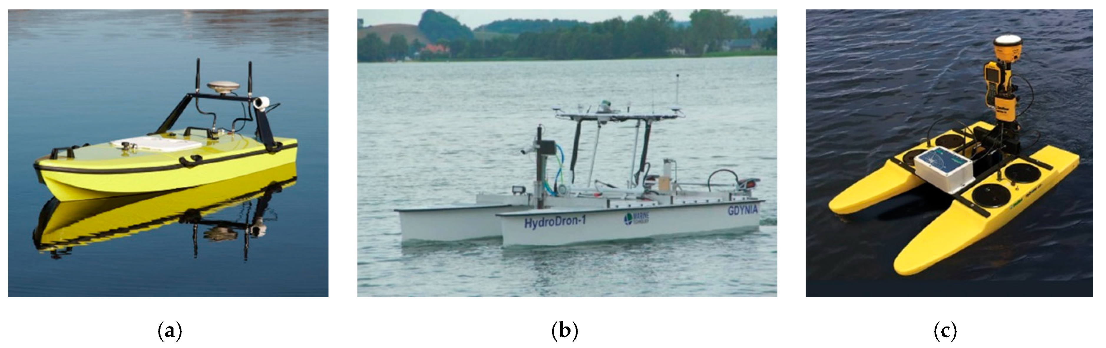
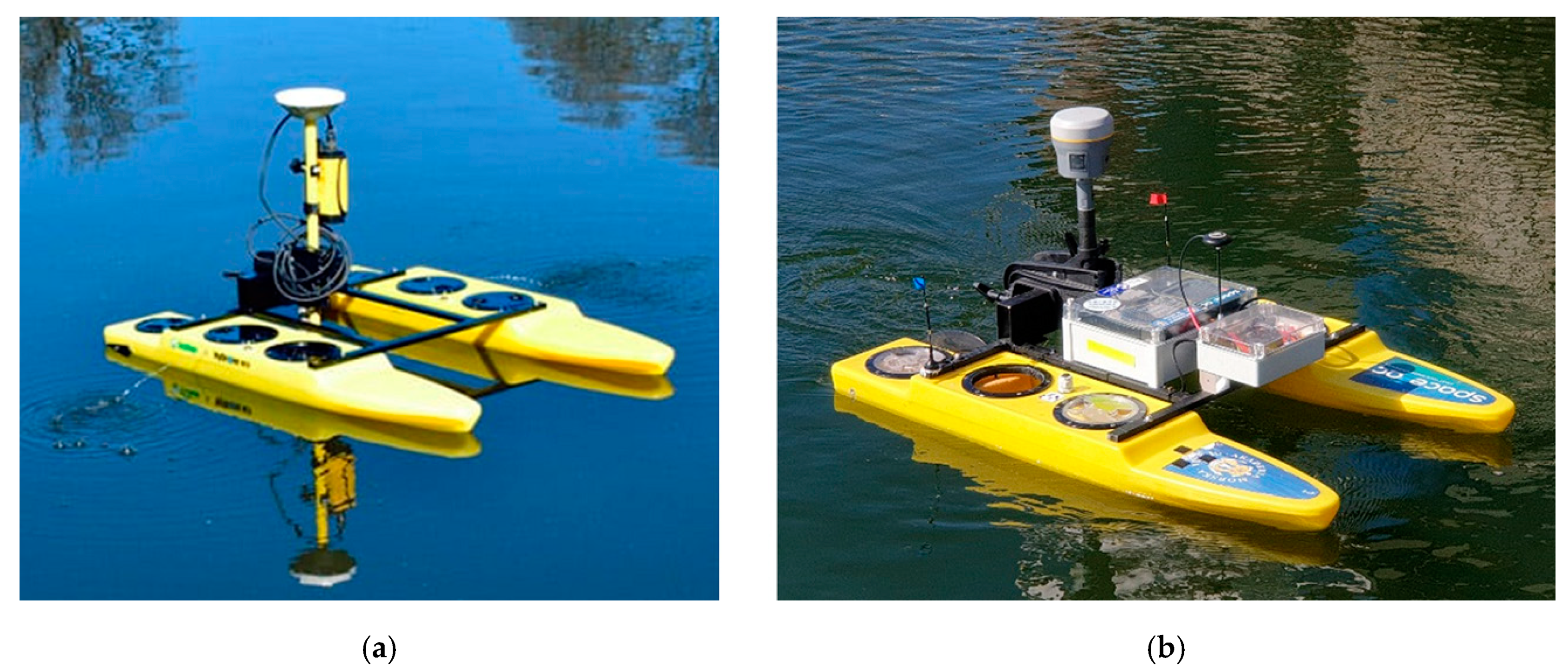
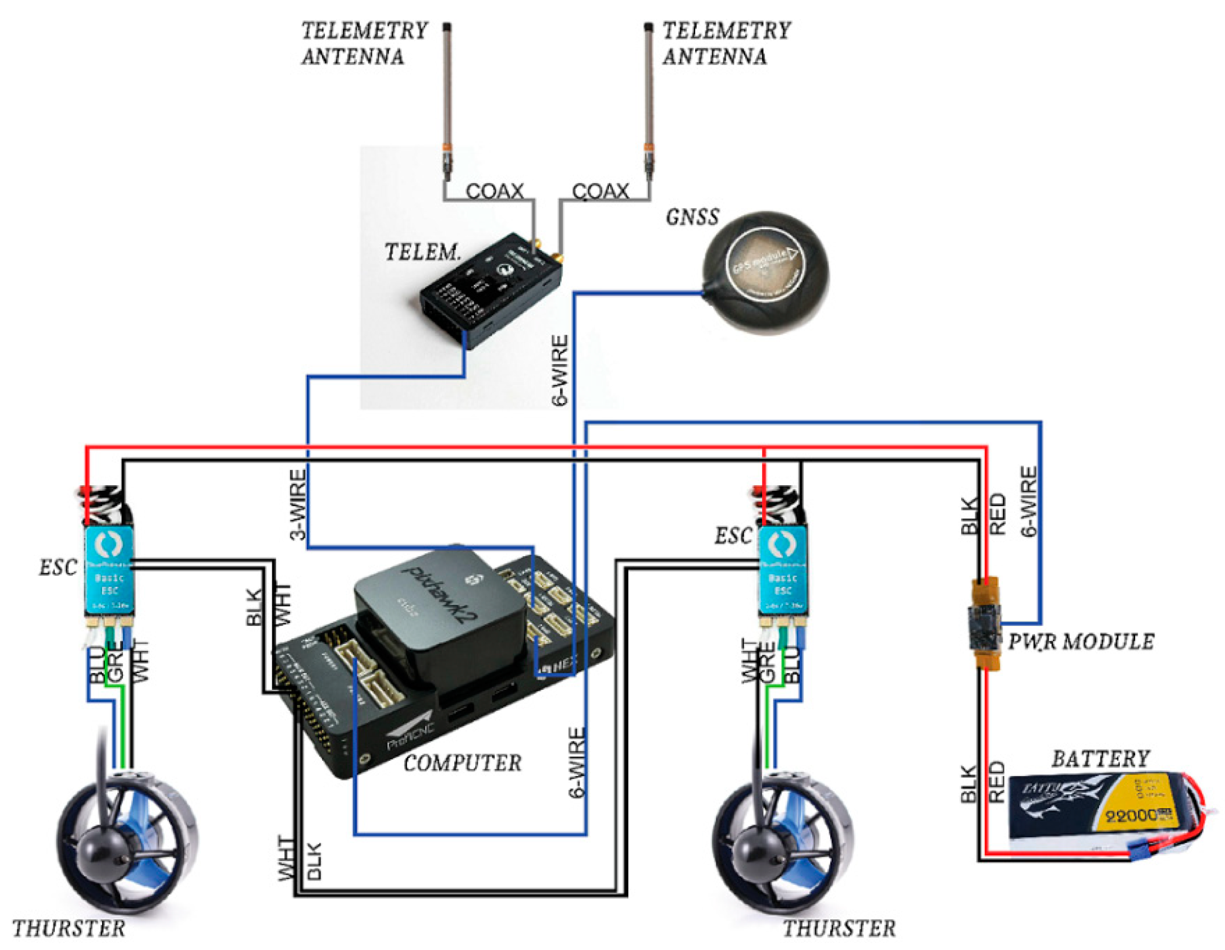
2.1. USV Modernisation
- Enable the performance of hydrographic measurement campaigns in automatic mode involving independent (with no operator’s participation) sailing along the planned sounding profiles;
- Improve the operating parameters and functionality through increasing the operating range, extending the operation time, and enhancing the reliability characteristics of both particular components and the entire system.
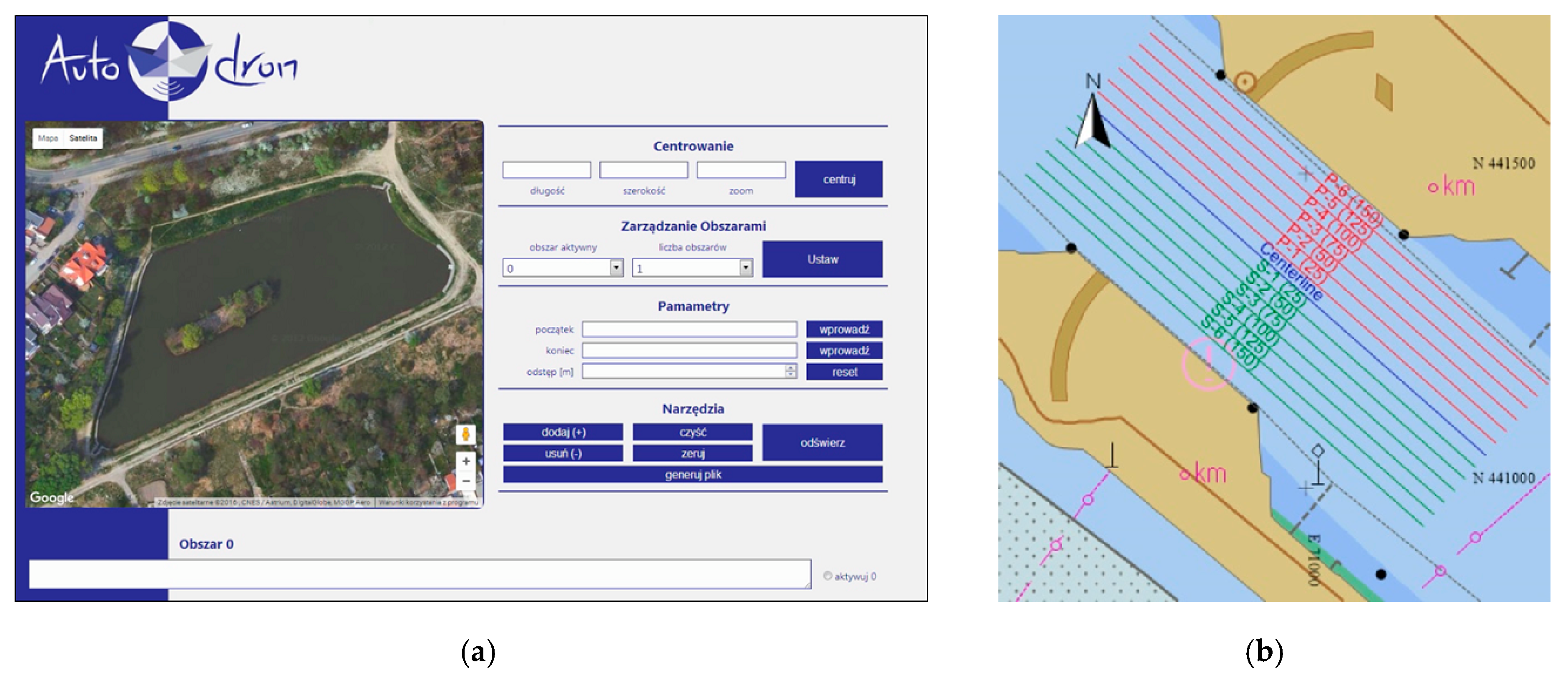
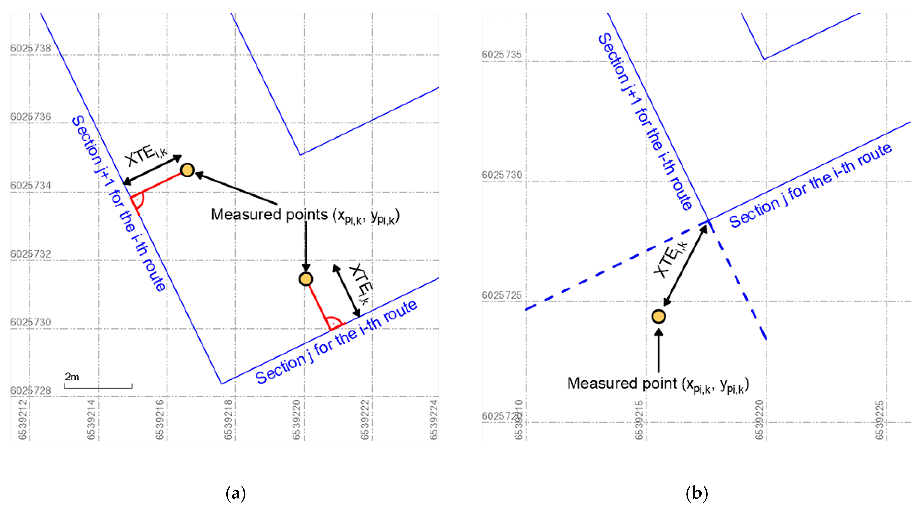
2.2. Measurements
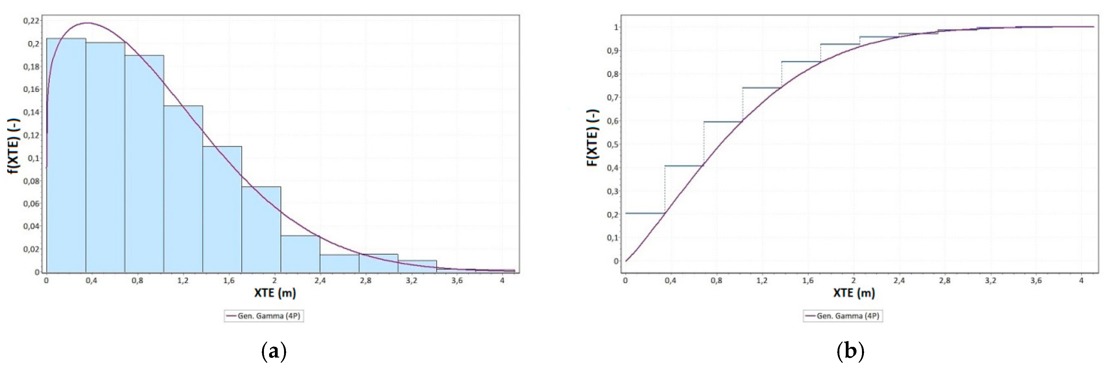
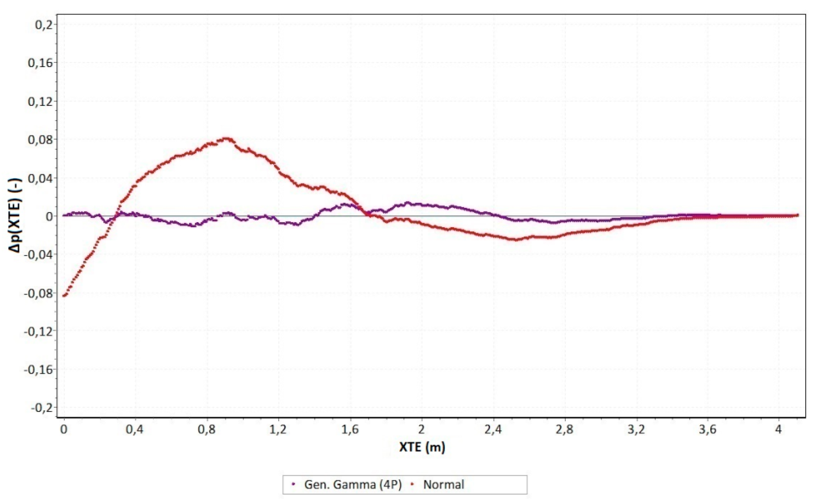
3. Results
4. Discussion
5. Conclusions
Author Contributions
Funding
Conflicts of Interest
References
- IHO. Hydrographic Dictionary, 5th ed.; Vol. I, Special Publication No. 32; IHO: Monaco, Monaco, 1994. [Google Scholar]
- CHS. CHS Hydrographic Survey Standards, 2nd ed.; CHS: Ottawa, ON, Canada, 2013. [Google Scholar]
- IHO. Manual on Hydrography, 1st ed.; Publication C-13; IHO: Monaco, Monaco, 2005. [Google Scholar]
- NOAA. NOS Hydrographic Surveys Specifications and Deliverables; NOAA: Silver Spring, MD, USA, 2017. [Google Scholar]
- Umbach, M.J. Hydrographic Manual, 4th ed.; NOAA: Silver Spring, MD, USA, 1976. [Google Scholar]
- IHO. IHO Standards for Hydrographic Surveys, 5th ed.; Special Publication No. 44; IHO: Monaco, Monaco, 2008. [Google Scholar]
- Stateczny, A.; Grońska, D.; Motyl, W. Hydrodron—New Step for Professional Hydrography for Restricted Waters. In Proceedings of the 2018 Baltic Geodetic Congress, Gdańsk, Poland, 21–23 June 2018. [Google Scholar]
- Bouwmeester, E.C.; Heemink, A.W. Optimal Line Spacing in Hydrographic Survey. Int. Hydrogr. Rev. 1993, 70, 37–48. [Google Scholar]
- Makar, A. Determination of Inland Areas Coastlines. In Proceedings of the 18th International Multidisciplinary Scientific GeoConference SGEM 2018, Albena, Bulgaria, 2–8 July 2018. [Google Scholar]
- Specht, C.; Weintrit, A.; Specht, M. Determination of the Territorial Sea Baseline—Aspect of Using Unmanned Hydrographic Vessels. TransNav-Int. J. Mar. Navig. Saf. Sea Transp. 2016, 10, 649–654. [Google Scholar] [CrossRef]
- Elema, I.A.; Kwanten, M.C. Introduction of Vertical Reference Level Lowest Astronomical Tide (LAT) in the Products of the Netherlands Hydrographic Service. In Proceedings of the 15th International Congress of the International Federation of Hydrographic Societies, Antwerp, Belgium, 6–9 November 2006. [Google Scholar]
- El-Hattab, A.I. Investigating the Effects of Hydrographic Survey Uncertainty on Dredge Quantity Estimation. Mar. Geod. 2014, 37, 389–403. [Google Scholar] [CrossRef]
- Peters, R.; Ledoux, H.; Meijers, M. A Voronoi-Based Approach to Generating Depth-Contours for Hydrographic Charts. Mar. Geod. 2014, 37, 145–166. [Google Scholar] [CrossRef] [Green Version]
- Russom, D.; Halliwell, H.R.W. Some Basic Principles in the Compilation of Nautical Charts. Int. Hydrogr. Rev. 1978, 55, 11–19. [Google Scholar]
- Stateczny, A.; Włodarczyk-Sielicka, M.; Grońska, D.; Motyl, W. Multibeam Echosounder and LiDAR in Process of 360-Degree Numerical Map Production for Restricted Waters with HydroDron. In Proceedings of the 2018 Baltic Geodetic Congress, Gdańsk, Poland, 21–23 June 2018. [Google Scholar]
- Moore, T.; Hill, C.; Monteiro, L. Is DGPS Still a Good Option for Mariners? J. Navig. 2001, 54, 437–446. [Google Scholar] [CrossRef]
- Dziewicki, M.; Specht, C. Position Accuracy Evaluation of the Modernized Polish DGPS. Pol. Marit. Res. 2009, 16, 57–61. [Google Scholar] [CrossRef]
- GSA. EGNOS Open Service (OS) Service Definition Document; Version 2.3; GSA: Prague, Czech Republic, 2017. [Google Scholar]
- Specht, C.; Pawelski, J.; Smolarek, L.; Specht, M.; Dąbrowski, P. Assessment of the Positioning Accuracy of DGPS and EGNOS Systems in the Bay of Gdansk Using Maritime Dynamic Measurements. J. Navig. 2019, 72, 575–587. [Google Scholar] [CrossRef]
- Wróbel, K.; Montewka, J.; Kujala, P. System-Theoretic Approach to Safety of Remotely-Controlled Merchant Vessel. Ocean Eng. 2018, 152, 334–345. [Google Scholar] [CrossRef]
- Stateczny, A.; Kazimierski, W.; Burdziakowski, P.; Motyl, W.; Wisniewska, M. Shore Construction Detection by Automotive Radar for the Needs of Autonomous Surface Vehicle Navigation. Int. J. Geo-Inf. 2019, 8, 80. [Google Scholar] [CrossRef]
- Stateczny, A.; Burdziakowski, P. Universal Autonomous Control and Management System for Multipurpose Unmanned Surface Vessel. Pol. Marit. Res. 2019, 26, 30–39. [Google Scholar] [CrossRef] [Green Version]
- Li, C.; Jiang, J.; Duan, F.; Liu, W.; Wang, X.; Bu, L.; Sun, Z.; Yang, G. Modeling and Experimental Testing of an Unmanned Surface Vehicle with Rudderless Double Thrusters. Sensors 2019, 19, 2051. [Google Scholar] [CrossRef] [PubMed]
- Romano, A.; Duranti, P. Autonomous Unmanned Surface Vessels for Hydrographic Measurement and Environmental Monitoring. In Proceedings of the FIG Working Week, Rome, Italy, 6–10 May 2012. [Google Scholar]
- Specht, C.; Specht, M.; Cywiński, P.; Skóra, M.; Marchel, Ł.; Szychowski, P. A New Method for Determining the Territorial Sea Baseline Using an Unmanned, Hydrographic Surface Vessel. J. Coast. Res. 2019, 35, 925–936. [Google Scholar] [CrossRef]
- Specht, C.; Świtalski, E.; Specht, M. Application of an Autonomous/Unmanned Survey Vessel (ASV/USV) in Bathymetric Measurements. Pol. Marit. Res. 2017, 24, 36–44. [Google Scholar] [CrossRef] [Green Version]
- Beirami, M.; Lee, H.Y.; Yu, Y.H. Implementation of an Auto-Steering System for Recreational Marine Crafts Using Android Platform and NMEA Network. J. Korean Soc. Marit. Eng. 2015, 39, 577–585. [Google Scholar] [CrossRef]
- Rajinikanth, V.; Latha, K. I-PD Controller Tuning for Unstable System Using Bacterial Foraging Algorithm: A Study Based on Various Error Criterion. Appl. Comput. Intell. Soft Comput. 2012, 2012, 1–10. [Google Scholar] [CrossRef] [Green Version]
- ISO. ISO 12188-2:2012—Tractors and Machinery for Agriculture and Forestry—Test Procedures for Positioning and Guidance Systems in Agriculture—Part 2: Testing of Satellite-Based Auto-Guidance Systems during Straight and Level Travel; ISO: Geneva, Switzerland, 2010. [Google Scholar]
- Rounsaville, J.; Dvorak, J.; Stombaugh, T. Methods for Calculating Relative Cross-Track Error for ASABE/ISO Standard 12188-2 from Discrete Measurements. Trans. ASABE 2016, 59, 1609–1616. [Google Scholar] [Green Version]
- USN. The Navy Unmanned Surface Vehicle (USV) Master Plan. Available online: https://www.navy.mil/navydata/technology/usvmppr.pdf (accessed on 24 July 2019).
- NGA. Department of Defense World Geodetic System 1984, Its Definition and Relationships with Local Geodetic Systems, 3rd ed.; NGA: Springfield, VA, USA, 2004. [Google Scholar]
- Deakin, R.E.; Hunter, M.N.; Karney, C.F.F. The Gauss-Krüger Projection. In Proceedings of the 23rd Victorian Regional Survey Conference, Warrnambool, Australia, 10–12 September 2010. [Google Scholar]
- Gajderowicz, I. Map Projections: Basics; Publishing House of the University of Warmia and Mazury in Olsztyn: Olsztyn, Poland, 2009. [Google Scholar]
- Kadaj, R.J. Polish Coordinate Systems. Transformation Formulas, Algorithms and Softwares. Available online: http://www.geonet.net.pl/images/2002_12_uklady_wspolrz.pdf (accessed on 24 July 2019).
- Hofmann-Wellenhof, B.; Lichtenegger, H.; Collins, J. Global Positioning System: Theory and Practice; Springer: New York, NY, USA, 1994. [Google Scholar]
- Stacy, E.W. A Generalization of the Gamma Distribution. Ann. Math. Stat. 1962, 33, 1187–1192. [Google Scholar] [CrossRef]
- Jaskólski, K.; Felski, A.; Piskur, P. The Compass Error Comparison of an Onboard Standard Gyrocompass, Fiber-Optic Gyrocompass (FOG) and Satellite Compass. Sensors 2019, 19, 1942. [Google Scholar] [CrossRef]
- Felski, A. Exploitative Properties of Different Types of Satellite Compasses. Annu. Navig. 2010, 16, 33–40. [Google Scholar]
- Liu, W.; Shi, X.; Zhu, F.; Tao, X.; Wang, F. Quality Analysis of Multi-GNSS Raw Observations and a Velocity-Aided Positioning Approach Based on Smartphones. Adv. Space Res. 2019, 63, 2358–2377. [Google Scholar] [CrossRef]
- Szot, T.; Specht, C.; Specht, M.; Dabrowski, P.S. Comparative Analysis of Positioning Accuracy of Samsung Galaxy Smartphones in Stationary Measurements. PLoS ONE 2019, 14, e0215562. [Google Scholar] [CrossRef]
- Wang, L.; Li, Z.; Zhao, J.; Zhou, K.; Wang, Z.; Yuan, H. Smart Device-Supported BDS/GNSS Real-Time Kinematic Positioning for Sub-Meter-Level Accuracy in Urban Location-Based Services. Sensors 2016, 16, 2201. [Google Scholar] [CrossRef]
- Specht, C.; Dąbrowski, P.S.; Pawelski, J.; Specht, M.; Szot, T. Comparative Analysis of Positioning Accuracy of GNSS Receivers of Samsung Galaxy Smartphones in Marine Dynamic Measurements. Adv. Space Res. 2019, 63, 3018–3028. [Google Scholar] [CrossRef]
- Fissore, F.; Masiero, A.; Piragnolo, M.; Pirotti, F.; Guarnieri, A.; Vettore, A. Towards Surveying with a Smartphone. In New Advanced GNSS and 3D Spatial Techniques; Springer: Cham, Switzerland, 2010; pp. 167–176. [Google Scholar]
- Dabove, P.; Di Pietra, V. Towards High Accuracy GNSS Real-Time Positioning with Smartphones. Adv. Space Res. 2019, 63, 94–102. [Google Scholar] [CrossRef]
- Chen, B.; Gao, C.; Liu, Y.; Sun, P. Real-Time Precise Point Positioning with a Xiaomi MI 8 Android Smartphone. Sensors 2019, 19, 2835. [Google Scholar] [CrossRef]
- Specht, M. Method of Evaluating the Positioning System Capability for Complying with the Minimum Accuracy Requirements for the International Hydrographic Organization Orders. Sensors 2019, 19, 3860. [Google Scholar] [CrossRef]
- Giordano, F.; Mattei, G.; Parente, C.; Peluso, F.; Santamaria, R. MicroVEGA (Micro Vessel for Geodetics Application): A Marine Drone for the Acquisition of Bathymetric Data for GIS Applications. Int. Arch. Photogramm. Remote Sens. Spat. Inf. Sci. 2015, 40, 123–130. [Google Scholar] [CrossRef]
- Giordano, F.; Mattei, G.; Parente, C.; Peluso, F.; Santamaria, R. Integrating Sensors into a Marine Drone for Bathymetric 3D Surveys in Shallow Waters. Sensors 2016, 16, 41. [Google Scholar] [CrossRef]


| A/O | Functionality | Before Modernisation | After Modernisation |
|---|---|---|---|
| A | Control | Direct RC | Direct RC, semi-automatic, automatic |
| A | RC operation range | 300 m (2400 MHz) | 1 km (868 MHz) |
| A | Telemetry monitoring | Additional PC | Integrated with the RC equipment |
| A | Positioning system | u-blox NEO-7: 56 channels; GPS, GLONASS, Galileo, QZSS, SBAS | u-blox NEO-M8N: 72 channels, GPS, GLONASS, BDS, Galileo, QZSS, SBAS |
| O | Possibility for hull replacement | No | Yes |
| O | Type of drive | Engines, main engine shafts, screws | Integrated pushing propellers 2 × 50 N |
| O | Engine cooling and ESC | Yes - forced, water | Not required |
| O | Battery bank | 2 × 9Ah AGM (2 × 10⁸ Wh) | 2 × 22 Ah LiPo (2 × 326 Wh) |
| O | Time of operation until battery replacement time | 1.5 h | 6 h |
| O | Vehicle weight | 25 kg | 18 kg |
| O | Ingress protection class | IP44 | IP56 |
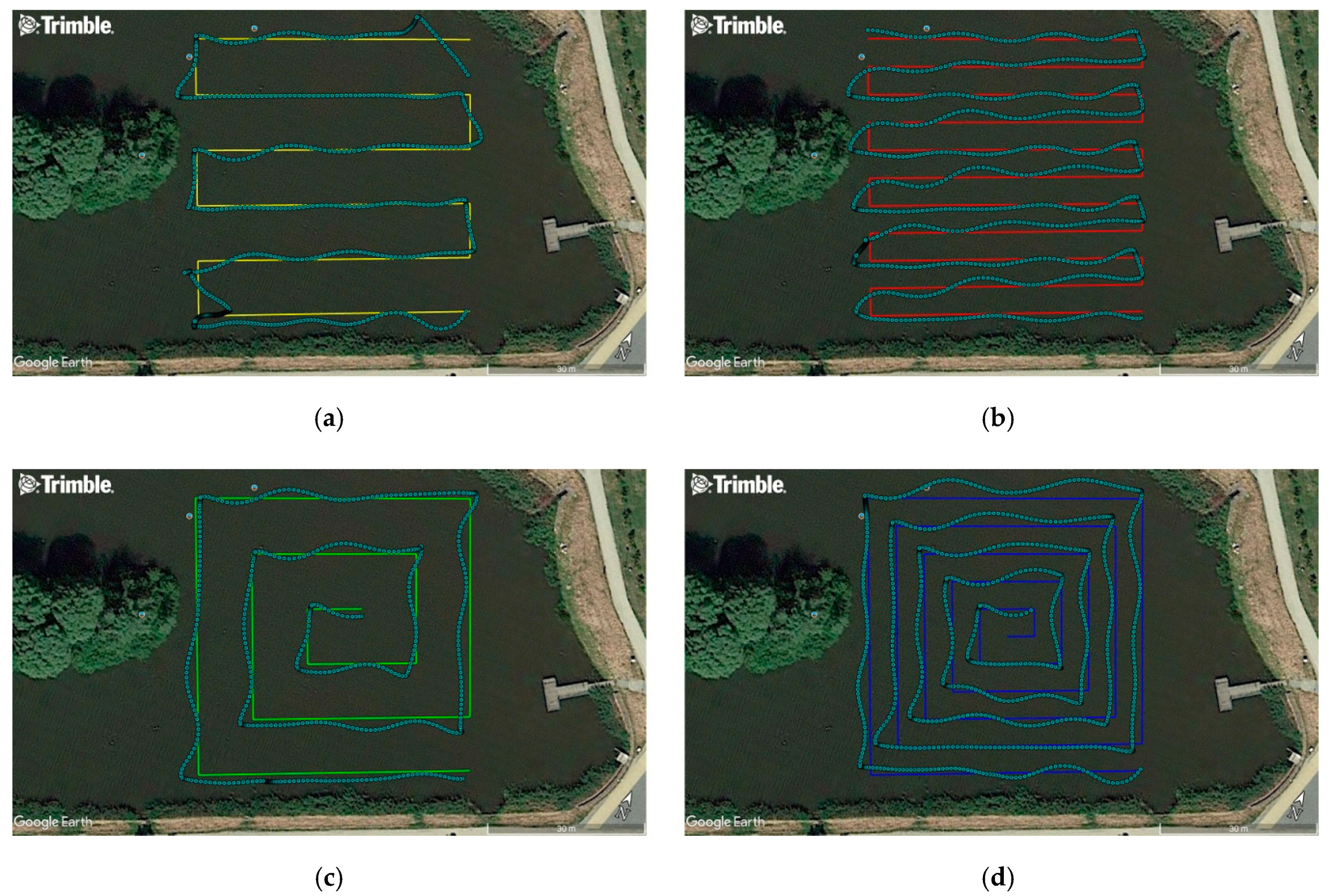
| Accuracy Measure | Route a (10 m) | Route b (5 m) | Route c (10 m) | Route d (5 m) |
|---|---|---|---|---|
| Route type |  |  |  |  |
| Number of measurements | 458 | 848 | 506 | 869 |
| XTE (p = 0.68) | 0.92 m | 1.15 m | 1.40 m | 1.27 m |
| XTE (p = 0.95) | 2.01 m | 2.38 m | 2.20 m | 2.39 m |
© 2019 by the authors. Licensee MDPI, Basel, Switzerland. This article is an open access article distributed under the terms and conditions of the Creative Commons Attribution (CC BY) license (http://creativecommons.org/licenses/by/4.0/).
Share and Cite
Specht, M.; Specht, C.; Lasota, H.; Cywiński, P. Assessment of the Steering Precision of a Hydrographic Unmanned Surface Vessel (USV) along Sounding Profiles Using a Low-Cost Multi-Global Navigation Satellite System (GNSS) Receiver Supported Autopilot. Sensors 2019, 19, 3939. https://0-doi-org.brum.beds.ac.uk/10.3390/s19183939
Specht M, Specht C, Lasota H, Cywiński P. Assessment of the Steering Precision of a Hydrographic Unmanned Surface Vessel (USV) along Sounding Profiles Using a Low-Cost Multi-Global Navigation Satellite System (GNSS) Receiver Supported Autopilot. Sensors. 2019; 19(18):3939. https://0-doi-org.brum.beds.ac.uk/10.3390/s19183939
Chicago/Turabian StyleSpecht, Mariusz, Cezary Specht, Henryk Lasota, and Piotr Cywiński. 2019. "Assessment of the Steering Precision of a Hydrographic Unmanned Surface Vessel (USV) along Sounding Profiles Using a Low-Cost Multi-Global Navigation Satellite System (GNSS) Receiver Supported Autopilot" Sensors 19, no. 18: 3939. https://0-doi-org.brum.beds.ac.uk/10.3390/s19183939