
Advanced Power Line Diagnostics Using Point Cloud Data—Possible Applications and Limits


Faculty of Electrical Engineering and Information Technology, University of Žilina, Univerzitná 1, 010 26 Žilina, Slovakia
*
Author to whom correspondence should be addressed.
Remote Sens. 2021, 13(10), 1880; https://0-doi-org.brum.beds.ac.uk/10.3390/rs13101880
Submission received: 1 April 2021
/
Revised: 3 May 2021
/
Accepted: 5 May 2021
/
Published: 11 May 2021
(This article belongs to the Special Issue Remote Sensing for Power Line Corridor Surveys)
Abstract
:The advance in remote sensing techniques, especially the development of LiDAR scanning systems, allowed the development of new methods for power line corridor surveys using a digital model of the powerline and its surroundings. The advanced diagnostic techniques based on the acquired conductor geometry recalculation to extreme operating and climatic conditions were proposed using this digital model. Although the recalculation process is relatively easy and straightforward, the uncertainties of input parameters used for the recalculation can significantly compromise such recalculation accuracy. This paper presents a systematic analysis of the accuracy of the recalculation affected by the inaccuracies of the conductor state equation input variables. The sensitivity of the recalculation to the inaccuracy of five basic input parameters was tested (initial temperature and mechanical tension, elasticity modulus, specific gravity load and tower span) by comparing the conductor sag values when input parameters were affected by a specific inaccuracy with an ideal sag-tension table. The presented tests clearly showed that the sag recalculation inaccuracy must be taken into account during the safety assessment process, as the sag deviation can, in some cases, reach values comparable to the minimal clearance distances specified in the technical standards.

1. Introduction
Electricity is one of the most important elements driving the technological development of our civilization. Electricity and its continuous delivery are critical for maintaining our current high standard of living and crucial for the modern industry.
For more than a century, a three-phase alternating current (AC) system is mostly used to transmit and distribute electricity. Using of a three-phase AC system has significant advantages. However, despite the rapid technological advancements in the field, due to the high parasitic capacitance of cables, it is still impractical (or impossible) to use underground cables to transmit electricity over long distances, especially at the transmission and sub-transmission level. Therefore, even modern power networks consist mainly of overhead power lines.
Representing a key element in the energy infrastructure, overhead power lines must be built in different terrain and climatic conditions. During their lifetime, overhead lines are exposed to severe weather conditions like strong wind, icing and significant temperature changes. Moreover, as the primary insulating medium is air, the safe operation of an overhead line can be compromised if the surrounding objects approach the phase conductors. A typical problem is vegetation growing under, or close to, power lines. Agricultural machines working on the fields crossed by the power lines represent another typical problem. Therefore, the conductor sag is a critical parameter that must be regularly checked.
It must be noted that the conductor sag is not a static parameter and can significantly change its value during the operation of the power line. The most important parameter influencing the size of the conductor sag is the temperature of the conductors. The conductor sag is also influenced by severe weather conditions like wind and icing. Moreover, conductor sag can increase due to changes in the mechanical properties of aging conductor. During the lifetime, the Aluminum Conductor Steel Reinforced (ACSR) conductors are exposed to the process of the permanent elongation known as a metallurgical creep. This elongation causes a gradual increase of the conductor sags in the individual spans of the power line.
Based on the above-mentioned reasons, it is necessary to make regular inspections of the overhead power lines and their corridors. Nowadays, most of the inspection methods are still based only on the visual inspection and assessment of the power line state by a walking technician, who performs the control. As the overhead power lines are linear structures, usually several tens to hundreds of kilometers long and are often located in difficult terrain conditions, the inspection is complicated and time-consuming. Therefore, in case of the long transmission lines, a helicopter is often used for a visual inspection of the power line state.
Based on the development of remote sensing methods, and particularly laser scanning techniques, more sophisticated methods have become available for power line inspections. Currently, aerial laser scanning using Light Detection and Ranging (LiDAR) technology represents a modern method for inspecting the overhead power lines. Due to the high reflectivity of the conductors and easy definability of their shape, aerial laser scanners can provide a comprehensive and realistic overview of the actual state of the scanned power line and its corridor. More detailed descriptions of the operation of LiDAR scanners and the possibilities of their use in the power line diagnostics are provided in the literature [1,2,3,4,5].
In general, the diagnostics of the power line state by using LiDAR technology can be performed by aerial laser scanning (ALS) or by terrestrial laser scanning (TLS). The advantages, disadvantages and the comparison of the ALS and TLS systems are described in [6,7].
The output from the ALS is a 3D point cloud, which consists of a large set of points representing the scanned scene. This raw point cloud is then processed using various specialized software tools. Individual points are classified according to the objects they belong to (ground, vegetation, building, tower, conductor, …) and optionally, essential objects are vectorized during the processing. It should be noted that the automatic point classification is still a very problematic task and extensive manual editing of the point cloud is still necessary to provide a high-quality digital model, significantly increasing the processing time and processing costs. Therefore, during the last decade, the research in the field of the ALS of the power lines was mainly focused on semi-automatic or automatic extraction and subsequent classification of points belonging to the power lines [8,9,10].
The extraction methods of the power line points can be divided into three groups, based on how the input points are grouped or classified into the individual objects in the scene. The methods involving the statistical analysis use height, density and the number of returned pulses [11,12,13,14]. Line-based methods use Hough transform and clustering based on 2D image processing [15] and RANdom Sample Consensus (RANSAC) [16,17,18]. Supervised classification-based methods first extract some features from input data and then apply the classification algorithm [19,20,21,22].
An essential part of the classification process is the detection and classification of points representing towers. The authors of the paper [23] present a tower reconstruction method from LiDAR data using stochastic geometry based on a model library. Another paper [24] presents a new approach to the extraction of conductors, towers and power line corridors based on the newly developed method of Height levels. The advantage of this method is a better extraction of vertically overlapping objects, e.g., trees and conductors.
Another branch of research in the field of the ALS is focused on the detection and classification of vegetation in the power line corridor, which may jeopardize the reliability and safety of the power line operation. Several algorithms have been developed in recent years to automatically detect the vegetation in the surroundings of the power line [25,26,27]. The simplest algorithms for classification of vegetation are based on the number of returns per a LiDAR pulse. During a single laser pulse from the scanner, the laser beam can reflect from multiple points at different heights. A typical scenario involves trees and higher vegetation, where the beam can hit several branches of a tree and also the ground below the tree. The logic is very simple. If there are multiple returns from a single pulse, the last return is evaluated as a ground point and all the previous returns are counted as vegetation. Of course, such classification is very crude and inaccurate. Therefore, this method is usually used as a rough classification routine for initial classification followed by a more sophisticated classification algorithm. Advanced classification methods are usually based on segmentation of the point cloud and analysis of point densities within the segment. A popular method is the analysis of vertical distribution of points within the segment. To avoid misclassification of points belonging to one object (for example a tree), but divided between two partial segments, the neighborhood growing method is often used.
Based on the correct classification of the vegetation points in the power line scan, it is possible to automatically search and visualize the dangerous parts of the vegetation extending to the proximity of the power line conductors, identify the most acute threats and improve the planning of the maintenance of the power line corridor (felling the dangerous vegetation) [28,29].
It must be noted that ALS is still a relatively new method of power line inspections, and in many scenarios, ALS is more expensive than the traditional inspection methods. To make it more attractive for the network operators and to justify the increased costs, it is necessary to extract from the digital model as much useful information as possible. However, as seen from the overview provided above, the most attention today is paid to development of the digital model itself and not how to use this model to support the network maintenance and operation.
The power line state during the ALS does not necessarily represent the most critical state of the operation from the point of view of minimal conductor distances from terrain or nearby objects. However, the complexity of the digital power line model acquired using ALS makes it possible to recalculate the conductor shape to any desired operation scenario, so the network operator can perform a complex safety evaluation of the power line in the wide range of scenarios, including climatic and operational extremes. The possibilities of the recalculation of the conductor shape to different atmospheric and operating conditions, based on the ALS data, are presented in [30].
At the first glance, such re-calculation is a relatively trivial task. However, the accuracy of such re-calculation is significantly affected by several factors, including point cloud accuracy, conductor temperature measurement/estimation accuracy and deviation of mechanical properties of conductors from declared values [31,32,33,34]. Understanding how these individual input inaccuracies affect the resulting accuracy of the recalculated conductor shapes is crucial for assessing the applicability of the method proposed in [30] (and, of course, all other possible applications based on solving of the conductor state equation and its derivatives). However (according to the best knowledge of authors), such analysis is not available in the literature.
2. Possible Use of Airborne LiDAR for Advanced Diagnostics of the Overhead Power Lines
Based on the 3D point cloud acquired by the ALS (and the digital model of the power line developed from this 3D point cloud), several advanced applications are possible to increase the value of acquired data for the network operator. These applications can significantly increase the awareness of the power line operator about the real safety conditions of the powerline and significantly improve the planning of necessary maintenance.
2.1. Determination of the Conductor Position Using ALS and Recalculation of Its Position to Arbitrary Climatic and Operating Conditions
The automated tools of various processing software (e.g., TerraScan, Mars, PLS-CADD) are able to determine and visualize the minimum height of the conductor above the terrain or other objects (vegetation, building, crossing of other power line, …) at the time of the power line scanning (Figure 1).
The commonly used commercial software tools are also able to evaluate the protection zone clearance at the time of the power line scanning. After defining the required clearance distance, the processing software search for points with distance to the conductor smaller than the specified value and can automatically change the class of these points to a danger point class. The process can be repeated for different clearance distance settings to search for points with different risk levels. The points with three different risk levels were identified in Figure 2. Cyan color represents points outside of the required clearance zone, but close to it. Purple color represents points within the clearance zone representing a medium risk to the power line and red color represents points dangerously close to the conductor. Such a classification is beneficial for the planning of maintenance works.
However, the determined minimal conductor height above the terrain, as well as the evaluation of the protection zone clearance are valid only for the conductor position at the time of the power line scanning. Since the conductor position varies due to the changes in ambient weather temperature during the day and season, as well as the conductor loading current, the scanned geometry of the conductor does not have to necessarily represent the worst-case sag scenario essential for the safety assessment. By using the appropriate equations, it is possible to recalculate the conductor position into any arbitrary climatic and operating conditions. Subsequently, as shown in Figure 3, the processing software allow to plot into the created model a new curve representing the conductor at the recalculated temperature (e.g., at +40 °C). Using the above-mentioned two automated tools, it is possible to check the minimum distances of conductors from terrain and the clearance of the protection zone with respect of the recalculated conductor position. However, the recalculation of the conductor position may be affected by specific errors of input parameters. Therefore, it is necessary to analyze the influence of input data errors on the resulting accuracy of the conductor recalculation.
2.2. Determination and Prediction of the Conductor Elongation Due to the Metallurgical Creep
When power lines that have been in operation for several years are scanned, it is very likely that the conductors will be elongated due to the metallurgical creep. It means that the conductor sag at the same temperature will be bigger than the sag immediately after the conductor installation. The value of the mechanical tension varies with the age of the conductor material. The sag-tension tables of the same power line will be different at the time of installation and at the time of the scanning after several years of the operation [35,36,37].
Using the processing software, it is possible to plot the vectorized curves of conductors from the scanned data concerning the operational conditions at the time of scanning. Subsequently, based on the theoretical calculations, it is possible to plot the conductor curve representing the post-installation state. Then, it is possible to determine the conductor elongation after a given period due to the metallurgical creep from the resulting sag differences. By comparing two scans after a specific period, it is possible to determine the dynamics of the conductor technical state changes. The significant advantage is that the conductor sags at the time of the scanning, at the time of the installation, and also in the future, can be easily plotted and compared in one model. Also, it should be noted that the determination of the conductor elongation due to the metallurgical creep is dependent on the correct recalculation of the conductor position.
2.3. Monitoring of the Tower Inclination and Deflection
The 3D power line model also allows to check towers for their deflections and inclination changes. An example of a medium voltage line tower scan with unusual inclination indicating a significant problem with the foundation of the tower is shown in Figure 4. It is also possible, in case of a high-resolution scan, to visually check for missing tower beams or other defects of the lattice construction of the tower.
Moreover, if the power line is scanned periodically, it is also possible to overlap the models acquired during the successive scanning campaigns and search for changes in the tower geometry or inclination during the time. It can significantly help to detect slowly developing problems early with the statics of the tower before the defect reaches a more critical level, potentially leading to the collapse of the structure.
In case there are some deformities detected on the tower, it is possible to perform a subsequent detailed scan with a terrestrial LiDAR system or by using an unmanned aerial vehicle (UAV). Based on the acquired high-resolution point cloud, it is possible to generate a 3D mesh model suitable for further structural analysis using the finite elements method (FEM). Such analysis can help accurately assess the severity of the detected problem and determine the most efficient problem solution. A similar approach was already tested to determine seismic vulnerability and safety assessment of buildings [38,39].
2.4. Other Possible Applications of Remote Sensing Methods for Power Line Corridor Maintenance Planning
The digital model of the power line corridor can also help to determine, predict, and monitor external risk like growing vegetation, landslides, or other terrain-related threats.
In combination with other remote sensing methods (e.g., infrared aerial imagery), it is possible to identify the type of vegetation growing under the power line, determine the terrain-given growth conditions and predict the growth speed [40,41]. Accurate prediction of vegetation growth can significantly improve the scheduling of maintenance of the power line corridor.
Another possible application is the analysis of terrain changes in areas with a high risk of landslides or rock falls. By comparing digital terrain models of the risk area from subsequent scans, it is possible to identify the developing threats and quantify the power line risk, allowing timely adoption of countermeasures [42].
3. Materials and Methods
As we can see from the previous section, there are several ways how to use the digital model of the power line acquired by aerial LiDAR scanning for safety assessment. Most of these applications are based on the modeling of the conductor geometry. Nevertheless, it is essential to note that the model of a conductor created from the point cloud represents only the operating conditions during the power line scanning and does not necessarily represent the worst-case scenario essential for safety assessment. However, if the operating conditions during the scanning are known with sufficient accuracy, it is possible to predict a conductor geometry during the worst-case scenario.
The shape of the conductor curve hanging between two support points can be described by the catenary equation or approximate parabolic equation. To better understand the methodology of analyses, presented later in this paper and the context of the conductor position recalculations, we present the following equations. These equations show the relationship among the geometry of the conductor, its mechanical parameters and additional mechanical loading. These equations can be found, for example, in literature [31,43,44].
The conductor catenary equation is given by the relation:
and the conductor parabolic equation is given by the relation:
where x and y are the coordinates of individual catenary points [m],
is the catenary parameter [m] and is equal to:
where is the conductor horizontal mechanical tension [MPa], is the conductor specific gravity load [N×m−3].
Considering the additional icing load, the catenary parameter can be calculated using the relation:
where is the conductor overloading factor caused by the icing [-]
where is the conductor self-gravity load [N×m−1], is the icing gravity load [N×m−1].
The conductor specific gravity load depends on the conductor self-gravity load and on the conductor cross-section :
Conductor self-gravity load q1 can be calculated by using the equation:
where is the conductor nominal specific weight [kg×m−1], is the gravitational acceleration constant (9.81×m×s−2).
The changes in conductor temperature and overloading by icing or wind will cause changes in the conductor mechanical tension and sag. The conductor state equation describes the relationship among the mechanical tension, temperature, additional loading, mechanical parameters of used conductor and the tower span. This paper deals with the mechanical calculations and the 2D conductor state equation without considering the additional wind load.
The conductor state equation is given by the Equation (8). The parameters marked with the index “0” represent the initial state and the parameters marked with the index “1” represent the final state:
where is the conductor horizontal mechanical tension [MPa], is the conductor temperature [°C], is the conductor overloading factor caused by icing [-], E is the conductor elasticity modulus [MPa], is the conductor specific gravity load [N×m−3], is the factor of linear thermal expansion of the conductor [°C−1].
Using the value of the mechanical tension obtained from the conductor state Equation (8), it is possible to calculate the maximum conductor sag [m] in the middle of the symmetrical tower span (both support points are at the same height):
The conductor state equation is also used for the calculation of sag-tension tables. These tables contain the mechanical tensions, sags and the corresponding temperatures. In this paper, the sag-tension tables were designed for temperatures in range of −30 °C to +70 °C, considering the possible climatic and operating conditions in the region of Slovakia.
When creating a sag-tension table of a new power line, the initial temperature of −5 °C with additional icing load (hereinafter marked as −5 °C*) is considered. This temperature corresponds to the initial mechanical tension of used conductor [MPa], which is calculated by using the equation:
where σDmax is the maximal permissible mechanical tension of used conductor [MPa].
The maximum conductor sag [m] corresponding to the mechanical tension and temperature −5 °C* is given by the equation:
The sag is calculated as the maximum sag, which can occur in the case of the icing in a given icing area. In practice, a smaller sag than the calculated sag value can occur at the temperature of −5 °C*, e.g., due to the lesser icing.
To perform the recalculation of the conductor position to any arbitrary climatic or operating conditions, it is necessary to know the conductor sag and mechanical tension during the ALS. In the case of using a LiDAR technology, the resulting conductor sag can be determined directly from the scan of the power line. The mechanical tension at the time of the power line scanning can be calculated based on the maximum conductor sag. The formula for calculation of the mechanical tension can be derived from Equation (9):
In the next part of the paper, the term “sag” (variable f with appropriate index) will indicate the maximum conductor sag in the middle of the symmetrical power line span.
We can easily recalculate the geometry of the conductor from the conditions at the time of the scanning to any desired operation scenario (different climatic conditions, current loading) by using the Equations (1)–(12). However, the accuracy of these calculations is questionable. Many of the required input parameters are only estimated in a real-world application or measured with relatively low accuracy. The real mechanical properties of conductors can also differ from the table values presented in datasheets provided by conductor manufacturers. These inaccuracies, or their combination, can lead to a significant error in conductor geometry estimation. Therefore, this paper is aimed at detailed analysis of the impacts of input inaccuracies that may affect the conductor geometry recalculation, thus, evaluating the practical usability of such conductor geometry recalculations for power line inspections.
All analyses mentioned in this paper were performed for one specific scenario, thus determining the methodology and accuracy of the conductor position recalculation and subsequently the evaluation of the sag deviations caused by the incorrect input parameters. The analyses assumed the power line with conductor ACSR 240/39, symmetrical tower span of 300 m, weak icing area N1 and no wind. Mechanical parameters of the ACSR conductor used in the calculations are summarized in the following Table 1.
Based on the mechanical parameters summarized in Table 1 and based on the relation (8), the state equation of the ACSR 240/39 conductor was modeled in Matlab software. The temperature of −5 °C* with additional icing load was chosen as an initial state. According to the Equation (10), the initial mechanical tension corresponding to the temperature of −5 °C* is = 93.426 MPa. Weak icing area N1 is represented by the icing gravity load of = 9.741 N×m−1. Subsequently, based on the conductor state Equation (8) and based on the equation for the sag calculation (9), the sag-tension table for the temperature range of −30 °C to +70 °C was calculated (Table 2). The calculated sag-tension Table 2 was chosen as the reference one. Based on the reference sag-tension table, the sag deviations that occur by the recalculation of the conductor position due to the incorrectly determined input parameter of the state equation, were evaluated.
After the calculation of the reference sag-tension table, the analysis of the influence of the conductor state equation input parameters inaccuracies on the resulting recalculation of the conductor position was performed. The analyzed parameters were as follows:
- the impact of the initial conductor temperature determination error,
- the impact of the conductor initial mechanical tension determination error,
- the impact of the conductor elasticity modulus determination error,
- the impact of the conductor specific gravity load determination error,
- the impact of the tower span determination error.
For each mentioned input parameter of the state equation, the sensitivity analysis was performed in such a way that only one particular input parameter was modified with a specific error while the other variables of the state equation remained unchanged. After modifying the particular parameter of the state equation with an appropriate error, new sag-tension tables were subsequently calculated. By comparing the new sag-tension tables and the reference sag-tension Table 2, the resulting sag differences that occur due to the incorrect determination of the state equation input parameter, were evaluated. Subsequently, from the positive and negative values of the sag deviations, the resulting maximum absolute and percentage sag deviations from the reference values were evaluated. In this paper, the absolute sag deviations are presented in more detail by tables and graphical interpretations, while the percentage sag deviations are presented only by graphical interpretations.
After the partial analyzes, where only one input parameter was modified with an error, a cumulation of input parameter errors that will cause the most significant sag deviation, was created and evaluated.
The term “sag deviation” refers to the difference between the original sag value from the reference sag-tension Table 2 and the recalculated sag values from the newly calculated sag-tension tables. This sag difference is caused by the recalculation of the conductor position to the arbitrary climatic and operating conditions due to the incorrectly determined input parameter of the conductor state equation.
The ALS of the power lines is mainly performed at good weather conditions, usually during the positive ambient temperatures. If the power line loading by the operating current is low, the ambient temperature can be considered as the conductor temperature (also in the case of no wind)—during hot summer months, the conductor temperature can reach the value of approx. +40 °C in the region of Slovakia. However, due to the higher current loading of the power line at the time of the scanning, the conductor temperature may not correspond to the ambient temperature. In the case of high current loading of the power line, and at the same time, at high ambient temperatures in hot summer months and no wind, the ACSR conductors can reach temperatures of +40 °C to +70 °C. From the point of view of power line diagnostics, the conductor temperature of +70 °C represents the most unfavorable state when the biggest conductor sag occurs. Therefore, in the following subsections, the range of sag deviations that occur due to the incorrectly determined parameter of the state equation and by the recalculation from temperatures +10–+60 °C to temperature +70 °C, was evaluated in more detail. Based on the above-mentioned facts, the conductor temperatures of +10 °C to +60 °C will most often occur during the power line scanning.
The main contribution of this paper is to determine the influence of the known inaccuracies of the state equation input parameters on the resulting recalculation of the conductor position for a specific scenario (ACSR 240/39, icing area N1, no wind, symmetrical tower span of 300 m). The magnitudes of the input parameter errors were obtained from [31,32,33,34] and are described in more detail in Section 4.1, Section 4.2, Section 4.3, Section 4.4, Section 4.5 and Section 4.6. Based on the paper [33], we found out that the coefficient of the linear thermal expansion α does not change significantly during the conductor operation. Therefore, this parameter will not have a significant effect on the correct recalculation of the conductor position.
4. Results
In this section, the impact of uncertainties of basic input parameters on the accuracy of the recalculated conductor sag will be systematically analyzed. The following subsections will analyze the impact of measurement errors and uncertainties of initial temperature, conductor initial mechanical tension estimation, modulus of elasticity, specific gravity load and tower span on the accuracy of the recalculated conductor sag.
4.1. The Impact of the Conductor Initial Temperature Determination Error on the Recalculated Conductor Sag
Temperature is a significant factor that affects the position of the conductor. When re-calculating the conductor position of the arbitrary climatic and operating conditions, it is essential to understand the exact temperature of the conductor at the time of the power line scanning. This temperature is used as the initial temperature ϑ0 for the recalculations. Possible errors in the determination of the conductor initial temperature could contribute to the inaccurate recalculation of the conductor position.
Nowadays, direct and indirect monitoring methods are used for the conductor temperature determination. Using the direct monitoring methods, the conductor temperature is measured directly, or by measuring the specific temperature-dependent parameter, such as the conductor sag, mechanical tension or distance from ground [32,45]. Using the indirect monitoring methods, the conductor temperature is obtained by applying a specific mathematical model that uses the measured weather parameters and loading current as input data [46,47]. When using a helicopter or UAV, it is possible to determine the exact conductor temperature at the time of scanning by using the thermographic measurement. In aircraft use, the exact determination of the conductor temperature is very difficult. For this reason, the indirect monitoring methods has to be used for the determination of the conductor temperature at the time of the power line scanning.
Measurements of weather conditions may contain some errors. Authors in paper [47] present that current methods for determining the conductor temperature from ambient weather data and loading current produce a standard error of ±2 °C with a confidence interval of 68.2%. However, in practice, more significant errors in the determination of conductor temperature can occur. Considering these findings, the conductor initial temperature ϑ0 was gradually modified with an error of ±2 °C, ±3 °C, ±4 °C and ±5 °C. All other parameters of the conductor state equation remained unchanged. The maximum absolute sag deviations Δfϑ, caused by the incorrect determination of the conductor initial temperature, are summarized in the following Table 3. Graphical interpretations of the achieved results are presented in Figure 5.
- the overall sag deviations vary from 6.1 cm to 18.9 cm (0.632%–3.053%);
- when recalculating data to high temperatures (e.g., +70 °C), the resulting sag deviations are smaller than when recalculating to low temperatures (e.g., −30 °C)→advantage from the point of view of the power line safety assessment;
- the resulting sag deviation does not depend on the initial temperature, the sag deviations are approximately the same for the initial temperature of −30 °C and + 30 °C;
- with an increasing conductor initial temperature determination error, the sag deviation increases linearly;
- the incorrect determination of the conductor initial temperature by ±5 °C will cause 2.5-times bigger sag deviation than the incorrect determination of the initial temperature by ±2 °C.
Considering the last point, following Figure 6 shows the increase of the sag deviations depending on the error magnitude in determining the initial conductor temperature. For better clarity, the curves are plotted only for two final temperatures ϑ1 (−30 °C and +70 °C).
The analyses performed in this subsection confirmed that errors in determination of the conductor initial temperature can significantly affect the resulting recalculation of its position to the arbitrary climatic and operating conditions. If the conductor initial temperature is incorrectly determined by more than ±2 °C, the resulting sag deviation may reach significant values. Therefore, in practice, it is essential to pay a sufficient attention to the correct determination of the conductor temperature at the time of the power line ALS.
4.2. The Impact of the Conductor Initial Mechanical Tension Determination Error on the Recalculated Conductor Sag
In order to recalculate the conductor position to the desired climatic and operating conditions, it is necessary to know the conductor mechanical tension at the time of the scanning, which is at the same time, the initial mechanical tension σH0 for recalculations. This initial mechanical tension can be determined from the conductor geometry using the Equation (12). In the case of the power line scanning by using a LiDAR technology, the accuracy of the conductor mechanical tension estimation depends on the overall accuracy of point cloud representing the power line corridor. Based on this knowledge, firstly, the verification of the point cloud accuracy was performed. Subsequently, the point cloud inaccuracy dependence on the initial mechanical tension determination and conductor position recalculation was examined.
4.2.1. Analysis of the Point Cloud Accuracy Representing the Power Line Corridor
The analyzed point cloud was obtained by the ALS of multiple power line corridors in the northern part of the Slovak Republic. A Piper Seneca III aircraft equipped with the Trimble Harrier 68i LiDAR scanner was used to scan the power lines in a target area. The power line scanning was realized from an altitude of approximately 650 m above the ground level at a speed of approx. 210 km/h. The target area was scanned multiple times, so the resulting density of 20–25 pts×m−2 was achieved. In the datasheet of scanner, the manufacturer decelerates the maximum measurement error ±25 cm in the horizontal direction and ±15 cm in the vertical direction.
To examine the accuracy of the scan, it was firstly necessary to determine how well the obtained point cloud represents an object with known dimensions. For this purpose, a road bridge located in the proximity of the scanned power lines was chosen. Verification of the point cloud accuracy was performed in such a way that some dimensions of the bridge obtained by the scanning were compared with the dimensions obtained by the real measurement. The differences between the scanned and real measured values will determine the real horizontal and vertical measurement error of the scanner. An aerial view of the analyzed road bridge is in Figure 7.
Figure 8 shows the cross-section view of a road bridge, which was created from the scanned point cloud in the TerraScan software. White color labels represent the scanned dimensions in meters and green color labels represent the real, measured dimensions.
As we can see in Figure 8, several dimensions of the bridge were compared, thus obtaining the real horizontal and vertical accuracy of the scanner Trimble Harrier 68i. The results are summarized in the following Table 4.
As follows from Figure 8, horizontal accuracy of the scanner was examined based on the width of the bridge and width of the upper part of the railing. According to Table 4, the differences between the scanned and measured values are approx. 19–24 cm. Vertical accuracy was examined based on the height of the bridge railing. The difference between the scanned and measured value is approx. 13 cm. As we can see in Figure 8, vertical accuracy of the scanner can be also confirmed based on the dispersion of points representing the straight asphalt—dispersion of approx. 12.2–12.5 cm.
According to these results, it seems the accuracy of the obtained point cloud is within the limits specified by the manufacturer. It must be noted that the accuracy of the point cloud can vary between different locations (even during a single scan). Moreover, the resulting accuracy of the acquired point depends on the accuracy of the scanner, as well as on the quality of postprocessing of the raw data. From this point of view, the examples presented in this chapter are intended just as a demonstration of the performance of an ALS system during a real mission.
For additional verification of the point cloud accuracy, the scanned and real measured dimensions of three beams of 400 kV transmission line tower were compared. Figure 9 shows the cross-section view of the analyzed tower in the TerraScan software. White color labels represent the dimensions in meters, which were obtained from the scanned point cloud from the processing software. Green labels represent the real, measured dimensions.
As we can see from Figure 9, the difference between the scanned and real measured distance of the upper beam is 12.8 cm, the lower beam is −4.8 cm and the sloping beam is 9 cm. By comparing the dimensions obtained from the point cloud and real measurement, it can be stated that the accuracy of the point cloud is well within the range declared by the manufacturer. In general, the average dispersion of points is approximately ±10 cm.
Last experiment indicates the accuracy of the conductor mapping by the scanner. In the scanned area, there is a 400 kV transmission line with bundled conductors formed by three ACSR conductors per phase. A fixed distance of 40 cm is formed between the individual conductors in the bundle by using the spacers with the shape of the equilateral triangle (Figure 10). The green triangles from Figure 10 represent the 40 cm spacers used on the 400 kV power line and the black dots represent the points obtained by the scanner representing the examined section of the conductor. To minimize the impact of the conductor curvature, a section near the lowest point of the sag curve was examined.
Figure 10 shows the dispersion of points representing the individual conductors in the bundle. The diameter of all point groups representing the conductor is less than 20 cm. Due to the fact that the distance between conductors must be 40 cm (as representing by the green triangles), the real position of conductor is always close to the middle of each point group.
4.2.2. The Impact of the Point Cloud Inaccuracy on the Estimation of the Conductor Initial Mechanical Tension and Its Recalculated Position
After the experiments mentioned in Section 4.2.1, an analysis of the impact of the point cloud inaccuracy on the determination of the initial mechanical tension, and thus also on the correct recalculation of the conductor position, was evaluated. The analyses were performed in such a way that in the first step, the sag values from the sag-tension Table 2 were modified by an error of ±0.25 m (the value specified for the biggest measurement error of the scanner Trimble Harrier 68i). In the second step, the incorrectly determined sags by ±0.25 m were substituted to the Equation (12). Solving the Equation (12), the mechanical tensions corresponding to the point cloud inaccuracy of ±0.25 m were calculated. In the third step, these calculated mechanical tensions were considered as the initial mechanical tensions to the state Equation (8). Subsequently, by solving the state Equations (8) and (9), new recalculated conductor sags were determined and compared with the sag values from the reference sag-tension Table 2.
Following, Table 5 shows the resulting absolute sag deviations Δfσ caused by the incorrectly determined initial mechanical tension (due to the maximum inaccuracy of the scanner Trimble Harrier 68i). Graphical interpretations of the achieved results are presented in Figure 11. The analyzes were performed for all initial temperatures from the sag-tension table because the resulting sag deviation varies depending on which initial temperature ϑ0 [°C] to which final temperature ϑ1 [°C] the recalculation is performed.
- the overall sag deviations vary from 20.2 cm to 31.2 cm (2.099–5.040%);
- the biggest sag deviation of 31.2 cm occurs at recalculation from initial temperature of +70 °C to final temperature of −30 °C;
- the sag deviations of 21.7–24.4 cm (2.255–2.541%) occur at recalculations from initial temperatures of +10–+60 °C to final temperature +70 °C→disadvantage.
Considering the last point, these values are not negligible, and in combination with other inaccuracies of input parameters, can significantly affect the accuracy of the conductor position recalculation.
It must also be noted that some software tools are using a vectorized catenary string to represent a conductor for further analyzes (determining the distance from the ground, clearance distance, conductor sag). In that case, the accuracy of the recalculation process will be affected also by the accuracy of the vectorization routine.
In practice, it would be appropriate to examine the accuracy of the obtained point cloud after the power line scanning, e.g., by comparing the real and scanned dimensions of the objects located in the proximity of the scanned power line (tower, building, …). Such analysis would determine the accuracy of the obtained point cloud and the conductor position recalculation accuracy.
4.3. The Impact of the Conductor Elasticity Modulus Determination Error on the Recalculated Conductor Sag
The conductor elasticity modulus was another analyzed parameter. The variations of the elasticity modulus should be considered, mainly due to the variations in the technology of the conductor production and also due to the loading changes of conductor during the normal operation [31,33]. The inaccuracy of the conductor elasticity modulus can lead to an incorrect re-calculation of the conductor position to the arbitrary climatic and operating conditions.
According to the research presented in paper [33], we found that the determination error of the conductor elasticity modulus is not exceeded during the conductor lifetime the level of approx. ±10%. Based on this finding, the tabular value of the elasticity modulus of the conductor ACSR 240/39 was modified with an error of ±10% (±7386.1 MPa), while the other parameters of the state equation remained unchanged.
Following Table 6 summarizes the achieved maximum absolute sag deviations ΔfE, which were caused by the recalculation of the conductor position due to the incorrect determination of the conductor elasticity modulus by ±10%. Graphical interpretations of the achieved results are presented in Figure 12. The analyses were performed for all initial temperatures from the sag-tension table, because the resulting sag deviation varies depending on which initial temperature ϑ0 [°C] to the final temperature ϑ1 [°C] the recalculation is performed.
- the overall sag deviations vary from 0.3 cm to 6.4 cm (0.033–1.034%);
- the biggest sag deviation of 6.4 cm occurs at recalculation from initial temperature of +70 °C to final temperature of −30 °C;
- the decreasing sag deviations of 2.4–0.3 cm (0.254–0.033%) occur at recalculations from initial temperatures of +10–+60 °C to final temperature +70 °C.
Based on the results mentioned in this subsection, it can be stated that the elasticity modulus determination error of ±10% has a minimal effect on the correct re-calculation of the conductor position and can be completely neglected.
4.4. The Impact of the Conductor Specific Gravity Load Determination Error on the Recalculated Conductor Sag
The incorrect determination of the conductor specific gravity load γ may also affect the re-calculation of the conductor position to the arbitrary climatic and operating conditions. The authors in paper [31] stated that during the normal operation, the conductor weight slightly increases due to the dirt and moisture [31]. As follows from Equations (6) and (7), the conductor specific gravity load γ is proportional to conductor self-gravity load q1 and also to nominal specific conductor weight g1. According to the research presented in the paper [31] we found out that during the conductor lifetime, the specific conductor weight g1 may differ from the tabular value in the range of 0.2–0.6%.
To cover the worst-case scenario and based on the findings mentioned above, the tabular value of the specific gravity load γ of the conductor ACSR 240/39 was modified with an error of ±1% (±342.7 N×m−3), while the other parameters of the state equation remained unchanged. It has to be noted that the tabular value of the conductor specific gravity load γ was modified with an error of ±1% not only in the state Equation (8), but also in Equation (9) for the conductor sag calculation.
The achieved maximum absolute sag deviations Δfγ, which were caused by the recalculation of the conductor position due to the incorrect determination of the conductor specific gravity load by ±1%, are shown in the following Table 7. Graphical interpretations of the achieved results are presented in Figure 13. The analyzes were performed for all initial temperatures from the sag-tension table, as the resulting sag deviation varies depending on from which initial temperature ϑ0 [°C] to which final temperature ϑ1 [°C] the recalculation is performed.
- the overall sag deviations vary from 4.5 cm to 12.6 cm (0.469–2.026%);
- the biggest sag deviation of 12.6 cm occurs at recalculation from initial temperature of +70 °C to final temperature of −30 °C;
- the sag deviations of 6.4–9.1 cm (0.668–0.943%) occur at recalculations from initial temperatures of +10–+60 °C to final temperature +70 °C.
The sag deviations caused by the incorrect determination of the conductor specific gravity load γ by ±1% are not so substantial. However, the combination with other inaccuracies of the input parameters may significantly affect the resulting accuracy of the conductor position recalculation.
4.5. The Impact of the Tower Span Determination Error on the Recalculated Conductor Sag
The inaccuracies in determining the tower span could also contribute to the incorrect recalculation of the conductor position. When designing a new power line or creating a new sag-tension table, the tower span is defined as the horizontal distance between the conductor support points (the horizontal distance from the axis of the tower A to the axis of the tower B). From this definition follows that calculations of the conductor mechanics neglect the influence of the insulators and insulator strings. In the case of support towers, the insulators are in a vertical position, and thus, approximately in the axis of the tower. The problem occurs in the case of the anchor towers, where insulators are almost in the horizontal position (Figure 14). Then, the real tower span between the anchor and support tower is shorter than the designed distance. Due to the smaller span value, the deviations in the resulting recalculated conductor sags can occur.
To cover the worst-case scenario and based on the findings mentioned above, the reference tower span of 300 m was modified with an error of −2.5 m. Other parameters of the conductor state equation remained unchanged. For calculation simplicity, only a symmetrical tower span was considered. The value of 2.5 m represents the typical length of the anchor insulator string used on 110 kV distribution power lines in the Slovak Republic. It has to be noted that the reference value of the tower span was modified with an error of −2.5 m not only in the state Equation (8) but also in the Equation (9) for the conductor sag calculation.
Following Table 8 summarizes the achieved maximum absolute sag deviations Δfa, which were caused by the recalculation of the conductor position due to the incorrect determination of the tower span by −2.5 m. Graphical interpretation of the achieved results is presented in Figure 15. The analyzes were performed for all initial temperatures from the sag-tension table, because the resulting sag deviation varies depending on from which initial temperature ϑ0 [°C] to which final temperature ϑ1 [°C] the recalculation is performed.
- the overall sag deviations vary from 10.5 cm to 16 cm (1.227–2.535%);
- the biggest sag deviations of 15.7–16 cm occur at recalculation from initial temperature of +70 °C to final temperature of −30 °C;
- when recalculating from higher initial temperatures, the magnitudes of sag deviations change only minimally depending on the final temperature to which the recalculation is performed (e.g., recalculation from +70 °C—the difference is only 0.3 cm);
- when recalculating from low initial temperatures, the sag deviations change more significantly depending on the final temperature to which the recalculation is performed (e.g., recalculation from −30 °C—the difference is 1.3 cm);
- the higher sag deviations of 13.4–15.6 cm (1.395–1.626%) occur at recalculations from initial temperatures of +10–+60 °C to final temperature +70 °C→disadvantage.
Considering the last bullet, especially in combination with other inaccuracies of input parameters, the resulting accuracy of the conductor position recalculation can be affected more significantly. Therefore, in practice, it would be advantageous to consider the span value that corresponds to the horizontal distance between the conductor anchorage on the insulator of the anchor tower A and the conductor anchorage on the insulator of the support tower B. This would eliminate the span determination error and the re-calculation of the conductor position would be more accurate.
At the end of this subsection, it should also be emphasized that the lengths of the insulator strings on the 220 kV and 400 kV transmission lines are longer than the lengths of the insulator strings used on the 110 kV distribution lines. Therefore, it is necessary to consider a more significant error in the tower span determination in case of a transmission line analysis.
4.6. The Impact of Cumulation of Errors of the State Equation Parameters on the Recalculated Conductor Sag
The influence of inaccuracies of the individual input parameters of the conductor state equation on the resulting conductor position recalculation in the previous subsection was examined only by the “per-partes” method. This fact means that only one input variable was modified with an error, while the other variables remained unchanged. However, in practice, several input parameters can be incorrectly determined at the same time. The resulting sag deviation can be considerably bigger in comparison with the state when only one input parameter is modified with an error. Therefore, this part of the paper is focused on the cumulation of the inaccuracies of the state equation input parameters, which may affect the resulting recalculation of the conductor position.
The impact of combined inaccuracies was investigated using the tools of error analysis theory. According to the theory of propagation of uncertainties [48], for a general function of multiple variables , if all uncertainties are independent and random, the resulting uncertainty can be expressed as:
where , , are the uncertainties of variables , , .
is the resulting uncertainty of .
In case the uncertainties of input variables are not independent, we can use a more general formula [48]:
During this analysis, the combined effect of uncertainties of initial conductor sag “”, initial conductor temperature “”, conductor modulus of elasticity “E”, conductor specific gravity load “” and tower span “” on the uncertainty of resulting conductor sag “” at a given temperature “” was investigated.
The recalculation process is based on solution of conductor state Equation (8), however the conductor sag is not directly involved in this equation. Therefore, the first step is the estimation of the initial mechanical tension , based on the initial conductor sag using Equation (12). Next, we need to calculate the uncertainty of . Using the uncertainty propagation theory, it can be calculated as:
In the next step, we need to calculate the mechanical tension in the final state σH1. It can be calculated based on Equation (8), however because Equation (8) is basically a cubic equation, it is not possible to use this equation directly. The solution of Equation (8) must be expressed analytically using the cubic formula. It must be noted, that with respect to the number of independent variables in Equation (8), the resulting analytical formula for the solution using the cubic formula is extremely complex for a manual calculation and using of a SAS (Symbolic Algebra System) software is necessary! In this work, we used the Matlab with Symbolic Math Toolbox for the calculations.
Using the analytical formula for σH1, formulas for its partial derivations , , , and were derived using the SAS software. When all partial derivations are known, we can define the uncertainty of based on Equation (14) as:
The quadratic form was not used, because in this case, the uncertainties are not independent (the value of is a function of an ).
Finally, using the calculated final mechanical tension σH1 and its uncertainty , we can calculate the final conductor sag using Formula (9). The related uncertainty can be calculated similarly to Equation (15), but in this case, the uncertainties of input variables are not independent, so the resulting uncertainty can be calculated as:
To demonstrate the impact of the uncertainties of the five basic input parameters on the determination of the recalculated conductor sag, a set of calculations was performed. During the calculations, the uncertainties of individual input parameters were set as follows:
- the initial conductor temperature uncertainty = ±5 °C,
- the initial conductor sag uncertainty = ±25 cm,
- the conductor elasticity modulus uncertainty = ± 0.1 ,
- the conductor specific gravity load uncertainty = ±0.01 ,
- the tower span uncertainty = ±2.5 m.
From the previous analyses, it is clear, that the uncertainty of the final sag is temperature dependent. Therefore, the resulting uncertainty of conductor sag was calculated for all combinations of initial and final temperature from the original sag-tension table.
The resulting uncertainties of for different combinations of initial and final temperature are presented in Table 9. The graphical representation of obtained results is shown in Figure 16.
A short summary of the above presented results:
- the resulting sag uncertainty vary from ±0.300 m to ±0.786 m (4.834–13.553 %);
- the biggest uncertainty of ±0.786 m occurs at recalculation from initial temperature of −30 °C to final temperature of +70 °C;
- with respect to the fact that the scanning is mostly performed when the ambient temperature is above 0 °C, we can expect maximal errors of the recalculated conductor sag up to ± 0.7 m.
As we can see from these results, the sag deviations caused by the combination of errors of individual input parameters may reach significant values (in this case, up to ±0.8 m). Such large uncertainties are comparable to the minimal clearance distance for a 110 kV power line and can significantly affect the results and validity of the safety assessment process.
From the analyses mentioned in individual subsections follows that the incorrect determination of initial mechanical tension and initial temperature have the most significant effect on the recalculation of conductor position.
5. Discussion
As we can see from the results presented in Section 4, the uncertainties of input parameters of the conductor state equation can significantly affect the results of the conductor geometry recalculation. A quick summary of the maximum sag deviations caused by the incorrect determination of the individual state equation parameters is provided in Table 10.
Although the sag deviations caused by inaccuracies of individual input parameters seem to be relatively small compared to the absolute value of the conductor sag, and when combined, the resulting sag deviation can reach significant values. Of course, all presented results are just an illustration of how big the recalculation error for a given scenario can be (symmetrical tower span 300 m, ACSR 240/39 conductor, icing area N1, no wind). For other power line configurations, these absolute values can differ significantly!
At this point, it must be noted that due to the non-linear nature of the conductor state equation, the resulting inaccuracy of the conductor geometry recalculation is not just a linear combination of the individual inaccuracies mentioned in Section 4. The mutual interaction of the individual inaccuracies is a very complex multidimensional problem. Moreover, some of the investigated parameters can be directly or indirectly related in a way where a specific combination of parameter errors is simply not possible (or at least not probable). On the other hand, some typical combinations of parameter deviations can lead to a state where the individual inaccuracies will compensate each other in their resulting influence. Therefore, more in-depth research is necessary to describe the impact and relations between these inaccuracies. Such a complex analysis is out of the scope of this paper.
Another important point worth mentioning is that in most cases, it makes more sense to compare the absolute value of the sag recalculation error with the required clearance distance, rather than to the correct value of the conductor sag. The clearance distance is the primary parameter evaluated during the power line safety assessment.
For example, according to the sag-tension table provided in Section 3 (Table 2), depending on the temperature, the conductor sag for this specific scenario differs from 6.2 to 9.6 m. A recalculation error of 0.786 m is quite significant compared to the maximal value of conductor sag 9.6 m (relative error 8.19%). When considering that the minimum required distance from vegetation directly under a 110 kV power line is according to [49] approximately 1 m, it is clear, that such recalculation is very crude from the power line safety evaluation point of view. The inaccuracy must be taken into account during the evaluation of clearance distances of the recalculated conductor.
In light of the facts mentioned above, it is clear that when trying to recalculate the conductor geometry to some extreme operating conditions for the power line safety assessment. It makes sense to work with the exact geometry obtained by the recalculation process only in the case where the input parameters are known with high accuracy. In a typical scenario, significant uncertainties of input parameters must be taken into account. In that case, when evaluating the power line safety distances, rather than using a single recalculated catenary string representing the conductor, we should think about a space of possible conductor geometries concerning the known inaccuracies of input parameters. Then, the clearance distance should be evaluated against the boundary of this space.
Moreover, the inaccuracy of the point cloud representing the ground, vegetation and other objects within the power line safety corridor must be taken into account when evaluating the height of the conductor over the ground and its clearance distances to other objects.
Another essential phenomenon not covered in the analysis provided in Section 4 is the influence of the wind. For simplicity, all presented results were calculated for windless conditions, so the recalculation of conductor geometry was reduced to a 2D problem. However, in real-world applications, the influence of the wind must be considered. Wind can affect the estimation of initial mechanical tension, conductor sag and cause a side-way deflection of the conductor, expanding the space of possible conductor locations. The influence of the wind is especially crucial for correcting the side clearance distance in areas with sloping terrain. Therefore, our future research will be focused on the recalculation of the conductor geometry using a 3D vector state equation, expanding the analyses provided in this paper.
6. Conclusions
Current advances in remote sensing methods allowed the development of new progressive methods for the power line corridor safety assessment using a digital model of the power line and its surroundings. The digital model allows performing the safety assessment in a new way, considering conditions at the time of the scanning and other (extreme) operating conditions. Based on these data, the power line operator can significantly improve maintenance planning, decrease costs and increase the operational safety of the power line. However, an important factor influencing the usability of such remote sensing-based assessment methods is the accuracy of the digital model acquired by the scanning and accuracy of the subsequent recalculation of the conductor geometry to a new operation state.
It is clear from the presented results that any attempt to recalculate the shape of a conductor to another operating state must consider significant uncertainties of input parameters used for the recalculation. Due to these uncertainties, the recalculated geometry of the conductor has only limited information value. Such a recalculation can provide some more or less crude estimation of the real conditions in the power line corridor, but there will always be a high probability of significant errors in the conductor geometry recalculation. The combined effect of all input parameter inaccuracies can cause errors in the recalculated conductor sag comparable with the minimum clearance distances specified in technical standards.
Based on these results, it seems that rather than a simple evaluation of corridor safety based on the recalculated conductor geometry, it is better to think about a space of possible conductor positions concerning all uncertainties of input parameters. Using this approach, the evaluation of the corridor safety should be based on the boundary of this space.
The purpose of this paper is to point out the most problematic impacts of input data inaccuracies and show the limits of assessment methods based on the recalculation of the conductor geometry. In this context, the remote sensing methods are not applicable only for the initial point cloud acquisition, classification, and vectorization. Remote sensing methods could also be used to determine the exact conductor temperature and meteorological conditions in the investigated area. These methods can also significantly contribute to lowering the uncertainties and increasing the accuracy of the power line corridor safety assessment based on a recalculation of the conductor geometry.
Author Contributions
Conceptualization and supervision: A.O.; methodology: M.H. and A.O.; Investigation and formal analysis: M.S. and M.H.; writing: M.S. and M.H.; LiDAR data processing: M.H.; funding acquisition: A.O. All authors have read and agreed to the published version of the manuscript.
Funding
This research received no external funding.
Institutional Review Board Statement
Not applicable.
Informed Consent Statement
Not applicable.
Data Availability Statement
Not applicable.
Acknowledgments
This work was supported by the project: “Broker center of air transport for transfer of technology and knowledge into transport and transport infrastructure, ITMS 26220220156”.
Conflicts of Interest
The authors declare no conflict of interest.
Nomenclature
| Abbreviations | |
| AC | Alternating Current |
| ACSR | Aluminum Conductor Steel Reinforced |
| ALS | Aerial Laser Scanning |
| FEM | Finite Elements Method |
| LiDAR | Light Detection and Ranging |
| RANSAC | Random Sample Consensus |
| TLS | Terrestrial Laser Scanning |
| UAV | Unmanned Aerial Vehlicle |
| Symbols | |
| tower span [m] | |
| catenary parameter [m] | |
| conductor diameter [mm] | |
| conductor elasticity modulus [MPa] | |
| maximum conductor sag representing the cumulation of the state equation input parameter errors [m] | |
| maximum conductor sag [m] | |
| maximum conductor sag at temperature of −5 °C and an additional icing load [°C] | |
| gravitational acceleration constant [m·s−2] | |
| nominal specific conductor weight [kg·m−1] | |
| conductor self-gravity load [N·m−1] | |
| icing gravity load [N·m−1] | |
| conductor cross-section [mm2] | |
| coordinates of individual catenary points [m] | |
| conductor overloading factor by icing [-] | |
| conductor overloading factor by icing in the state 0 [-] | |
| conductor overloading factor by icing in the state 1 [-] | |
| factor of linear thermal expansion of conductor [°C−1] | |
| conductor specific gravity load [N·m−3] | |
| maximal permissible mechanical tension of conductor [MPa] | |
| conductor horizontal mechanical tension [MPa] | |
| conductor horizontal mechanical tension in the state 0 [MPa] | |
| conductor horizontal mechanical tension at temperature of −5 °C and an additional icing load [MPa] | |
| conductor horizontal mechanical tension in the state 1 [MPa] | |
| conductor temperature in the state 0 [°C] | |
| conductor temperature in the state 1 [°C] | |
| conductor span determination error [m] | |
| point cloud determination error [m] | |
| conductor elasticity modulus determination error [%] | |
| conductor specific gravity load determination error [%] | |
| maximum absolute sag deviation caused by the incorrect determination of the tower span [m] | |
| maximum absolute sag deviation caused by the cumulation of the state equation input parameter errors [m] | |
| maximum absolute sag deviation caused by the incorrect determination of conductor elasticity modulus [m] | |
| maximum absolute sag deviation caused by the incorrect determination of the conductor self-gravity load [m] | |
| maximum absolute sag deviation caused by the incorrect determination of the conductor initial temperature [m] | |
| maximum absolute sag deviation caused by the incorrect determination of the conductor initial mechanical tension [m] | |
| maximum percentage sag deviation caused by the incorrect determination of the tower span [m] | |
| maximum percentage sag deviation caused by the cumulation of the state equation input parameter errors [m] | |
| maximum percentage sag deviation caused by the incorrect determination of conductor elasticity modulus [m] | |
| maximum percentage sag deviation caused by the incorrect determination of the conductor self-gravity load [m] | |
| maximum percentage sag deviation caused by the incorrect determination of the conductor initial temperature [m] | |
| maximum percentage sag deviation caused by the incorrect determination of the conductor initial mechanical tension [m] | |
References
- Li, X.; Guo, Y. Application of LiDAR technology in power line inspection. IOP Conf. Ser. Mater. Sci. Eng. 2018, 382, 052025. [Google Scholar] [CrossRef]
- Toschi, I.; Morabito, D.; Grilli, E.; Remondino, F.; Carlevaro, C.; Cappellotto, A.; Tamagni, G.; Maffeis, M. Cloud-based solution for nationwide power line mapping. ISPRS Int. Arch. Photogramm. Remote Sens. Spat. Inf. Sci. 2019, XLII-2/W13, 119–126. [Google Scholar] [CrossRef] [Green Version]
- Matikainen, L.; Lehtomäki, M.; Ahokas, E.; Hyyppä, J.; Karjalainen, M.; Jaakkola, A.; Kukko, A.; Heinonen, T. Remote sensing methods for power line corridor surveys. ISPRS J. Photogramm. Remote Sens. 2016, 119, 10–31. [Google Scholar] [CrossRef] [Green Version]
- You, A.; Wang, X.; Han, X.; Tang, D. Applications of LiDAR in patrolling electric-power lines. In Proceedings of the 2013 The International Conference on Technological Advances in Electrical, Electronics and Computer Engineering (TAEECE), Konya, Turkey, 9–11 May 2013; pp. 110–114. [Google Scholar]
- Ahmad, J.; Malik, A.S.; Xia, L.; Ashikin, N. Vegetation encroachment monitoring for transmission lines right-of-ways: A survey. Electr. Power Syst. Res. 2013, 95, 339–352. [Google Scholar] [CrossRef]
- Lehtomäki, M.; Kukko, A.; Matikainen, L.; Hyyppä, J.; Kaartinen, H.; Jaakkola, A. Power line mapping technique using all-terrain mobile laser scanning. Autom. Constr. 2019, 105, 102802. [Google Scholar] [CrossRef]
- Wang, Y.; Chen, Q.; Liu, L.; Li, X.; Sangaiah, A.K.; Li, K. Systematic Comparison of Power Line Classification Methods from ALS and MLS Point Cloud Data. Remote. Sens. 2018, 10, 1222. [Google Scholar] [CrossRef] [Green Version]
- Zhou, M.; Li, K.Y.; Wang, J.H.; Li, C.R.; Teng, G.E.; Ma, L.; Wu, H.H.; Li, W.; Zhang, H.J.; Chen, J.Y.; et al. Automatic extraction of power lines from UAV lidar point clouds using a novel spatial feature. ISPRS Ann. Photogramm. Remote Sens. Spat. Inf. Sci. 2019, IV-2/W7, 227–234. [Google Scholar] [CrossRef] [Green Version]
- Sohn, G.; Jwa, Y.; Kim, H.B. Automatic powerline scene classification and reconstruction using airborne lidar data. ISPRS Ann. Photogramm. Remote Sens. Spat. Inf. Sci. 2012, I-3, 167–172. [Google Scholar] [CrossRef] [Green Version]
- McLaughlin, R. Extracting Transmission Lines from Airborne LIDAR Data. IEEE Geosci. Remote Sens. Lett. 2006, 3, 222–226. [Google Scholar] [CrossRef]
- Liang, J.; Zhang, J.; Deng, K.; Liu, Z.; Shi, Q. A New Power-Line Extraction Method Based on Airborne LiDAR Point Cloud Data. In Proceedings of the 2011 International Symposium on Image and Data Fusion, Yunnan, China, 9–11 August 2011; pp. 1–4. [Google Scholar]
- Liu, Y.; Li, Z.; Hayward, R.; Walker, R.; Jin, H. Classification of Airborne LIDAR Intensity Data Using Statistical Analysis and Hough Transform with Application to Power Line Corridors. Digit. Image Comput. Tech. Appl. 2009, 462–467. [Google Scholar] [CrossRef] [Green Version]
- Zhu, L.; Hyyppä, J. Fully-Automated Power Line Extraction from Airborne Laser Scanning Point Clouds in Forest Areas. Remote Sens. 2014, 6, 11267–11282. [Google Scholar] [CrossRef] [Green Version]
- Guan, H.; Yu, Y.; Li, J.; Ji, Z.; Zhang, Q. Extraction of power-transmission lines from vehicle-borne lidar data. Int. J. Remote Sens. 2016, 37, 229–247. [Google Scholar] [CrossRef]
- Yan, G.; Li, C.; Zhou, G.; Zhang, W.; Li, X. Automatic Extraction of Power Lines From Aerial Images. IEEE Geosci. Remote Sens. Lett. 2007, 4, 387–391. [Google Scholar] [CrossRef]
- Guo, B.; Li, Q.; Huang, X.; Wang, C. An Improved Method for Power-Line Reconstruction from Point Cloud Data. Remote Sens. 2016, 8, 36. [Google Scholar] [CrossRef] [Green Version]
- Kurdi, F.T.; Landes, T.; Grussenmeyer, P. Hough-transform and extended RANSAC algorithms for automatic detection of 3d building roof planes from Lidar data. ISPRS Int. Arch. Photogramm. Remote Sens. Spat. Inf. Syst. 2007, XXXVI, 407–412. [Google Scholar]
- Sevgen, S.C.; Karsli, F. An improved RANSAC algorithm for extracting roof planes from airborne lidar data. Photogramm. Rec. 2020, 35, 40–57. [Google Scholar] [CrossRef]
- Kim, H.B.; Sohn, G. Point-based Classification of Power Line Corridor Scene Using Random Forests. Photogramm. Eng. Remote Sens. 2013, 79, 821–833. [Google Scholar] [CrossRef]
- Wang, Y.; Chen, Q.; Liu, L.; Zheng, D.; Li, C.; Li, K. Supervised Classification of Power Lines from Airborne LiDAR Data in Urban Areas. Remote Sens. 2017, 9, 771. [Google Scholar] [CrossRef] [Green Version]
- Wang, Y.; Chen, Q.; Li, K.; Zheng, D.; Fang, J. Airborne lidar power line classification based on spatial topological structure characteristics. ISPRS Ann. Photogramm. Remote. Sens. Spat. Inf. Sci. 2017, IV-2/W4, 165–169. [Google Scholar] [CrossRef] [Green Version]
- Yang, J.; Kang, Z. Voxel-Based Extraction of Transmission Lines from Airborne LiDAR Point Cloud Data. IEEE J. Sel. Top. Appl. Earth Obs. Remote Sens. 2018, 11, 3892–3904. [Google Scholar] [CrossRef]
- Guo, B.; Huang, X.; Li, Q.; Zhang, F.; Zhu, J.; Wang, C. A Stochastic Geometry Method for Pylon Reconstruction from Airborne LiDAR Data. Remote Sens. 2016, 8, 243. [Google Scholar] [CrossRef] [Green Version]
- Awrangjeb, M. Extraction of Power Line Pylons and Wires Using Airborne LiDAR Data at Different Height Levels. Remote Sens. 2019, 11, 1798. [Google Scholar] [CrossRef] [Green Version]
- Mills, S.J.; Castro, M.P.G.; Li, Z.; Cai, J.; Hayward, R.; Mejias, L.; Walker, R.A. Evaluation of Aerial Remote Sensing Techniques for Vegetation Management in Power-Line Corridors. IEEE Trans. Geosci. Remote Sens. 2010, 48, 3379–3390. [Google Scholar] [CrossRef]
- Jardini, M.G.M.; Jardini, J.A.; Crispino, F.; Simões, A.J.M.; De Souza, J.M.S.; Dos Santos, W.L. Vegetation detection close to transmission lines using cloud data points from lidar in Brazil. In Proceedings of the Modelling, Simulation and Identification/858: Intelligent Systems and Control, Calgary, AB, Canada, 16–17 July 2018. [Google Scholar] [CrossRef]
- Clode, S.; Rottensteiner, F. Classification of trees and powerlines from medium resolution airborne laserscanner data in urban environments. In Proceedings of the Workshop on Digital Image Computing 2005 (WDIC2005), Brisbane, Australia, 21 February 2005. [Google Scholar]
- Frank, M.; Pan, Z.; Raber, B.; Lenart, C. Vegetation management of utility corridors using high-resolution hyperspectral imaging and LiDAR. In Proceedings of the 2010 2nd Workshop on Hyperspectral Image and Signal Processing: Evolution in Remote Sensing, Reykjavik, Iceland, 14–16 June 2010; pp. 1–4. [Google Scholar]
- Chen, C.; Yang, B.; Song, S.; Peng, X.; Huang, R. Automatic Clearance Anomaly Detection for Transmission Line Corridors Utilizing UAV-Borne LIDAR Data. Remote Sens. 2018, 10, 613. [Google Scholar] [CrossRef] [Green Version]
- Zhang, S.C.; Liu, J.Z.; Niu, Z.; Gao, S.; Xu, H.Z.; Pei, J. Power Line Simulation for Safety Distance Detection Using Point Clouds. IEEE Access 2020, 8, 165409–165418. [Google Scholar] [CrossRef]
- CIGRE. Sag-Tension Calculation Methods for Overhead Lines; CIGRE: Paris, France, 2016; ISBN 978-2-85873-010-0. [Google Scholar]
- Lindberg, E. The Overhead Line Sag Dependence on Weather Parameters and Line Current. Master’s Thesis, Uppsala University, Uppsala, Sweden, 2011. [Google Scholar]
- Polevoy, A. Impact of Data Errors on Sag Calculation Accuracy for Overhead Transmission Line. IEEE Trans. Power Deliv. 2014, 29, 2040–2045. [Google Scholar] [CrossRef]
- Alvarez, D.L.; Da Silva, F.M.F.; Mombello, E.E.; Bak, C.L.; Rosero, J.A. Conductor Temperature Estimation and Prediction at Thermal Transient State in Dynamic Line Rating Application. IEEE Trans. Power Deliv. 2018, 33, 2236–2245. [Google Scholar] [CrossRef] [Green Version]
- Širanec, M.; Höger, M.; Otčenášová, A. Evaluation of power line parameter estimation accuracy based on data from airborne LiDAR. In Proceedings of the 10th International Scientific Symposium on Electrical Power Engineering, Elektroener-Getika 2019, Stará Lesná, Slovakia, 16–18 September 2019. [Google Scholar]
- Michael, M.; Stephan, P.; Stefan, J. Elongation of overhead line conductors under combined mechanical and thermal Stress. In Proceedings of the 2008 International Conference on Condition Monitoring and Diagnosis, Beijing, China, 21–24 April 2008; pp. 671–674. [Google Scholar]
- Albizu, I.; Mazón, A.J.; Fernandez, E. A method for the sag-tension calculation in electrical overhead lines. Int. Rev. Electr. Eng. 2011, 6, 1380–1389. [Google Scholar]
- Fortunato, G.; Funari, M.F.; Lonetti, P. Survey and seismic vulnerability assessment of the Baptistery of San Giovanni in Tumba (Italy). J. Cult. Heritage 2017, 26, 64–78. [Google Scholar] [CrossRef]
- Stepinac, M.; Gašparović, M. A Review of Emerging Technologies for an Assessment of Safety and Seismic Vulnerability and Damage Detection of Existing Masonry Structures. Appl. Sci. 2020, 10, 5060. [Google Scholar] [CrossRef]
- Nakajima, T.; Hirata, Y.; Hiroshima, T.; Furuya, N.; Satoshi, T.; Tsuyuki, S.; Shiraishi, N. A Growth Prediction System for Regional Forest Resources Derived from LiDAR Data; Silvilaser: College Station, TX, USA, 2009. [Google Scholar]
- Rybansky, M.; Brenova, M.; Cermak, J.; Van Genderen, J.; Sivertun, Å. Vegetation structure determination using LIDAR data and the forest growth parameters. In Proceedings of the IOP Conference Series: Earth and Environmental Science, Kuala Lumpur, Malaysia, 13–14 April 2016; Volume 37, p. 12031. [Google Scholar]
- Abellán, A.; Calvet, J.; Vilaplana, J.M.; Blanchard, J. Detection and spatial prediction of rockfalls by means of terrestrial laser scanner monitoring. Geomorphology 2010, 119, 162–171. [Google Scholar] [CrossRef]
- Otčenášová, A. Mechanics of Overhead Power Lines, EDIS; University Textbook; University of Žilina: Žilina, Slovakia, 2005; 236p, ISBN 978-80-554-0181-2. [Google Scholar]
- Varga, L.; Leščinský, P.; Beňa, Ľ. Calculation of Mechanical Conditions of Overhead Power Lines; University Textbook, Mercury-Smékal; Technical University of Košice: Košice, Slovakia, 2019; 187p, ISBN 80-89061-56-7. [Google Scholar]
- Pavlinic, A.; Komen, V. Direct monitoring methods of overhead line conductor temperature. Eng. Rev. 2017, 37, 134–146. [Google Scholar]
- Kanálik, M.; Margitová, A.; Beňa, Ľ. Temperature calculation of overhead power line conductors based on CIGRE Technical Brochure 601 in Slovakia. Electr. Eng. 2019, 101, 921–933. [Google Scholar] [CrossRef]
- Bockarjova, M.; Andersson, G. Transmission Line Conductor Temperature Impact on State Estimation Accuracy. In Proceedings of the 2007 IEEE Lausanne Power Tech, Lausanne, Switzerland, 1–5 July 2007; pp. 701–706. [Google Scholar]
- Taylor, J.R. An Introduction to Error Analysis, 2nd ed.; University Science Books: Sausalito, CA, USA, 1997; ISBN 0-935702-75-X. [Google Scholar]
- EN 50341-1:2012. Overhead Electrical Lines Exceeding AC 1 kV—Part 1: General Requirements—Common Specifications; CENELEC: Brussels, Belgium, 2012. [Google Scholar]
Figure 1.
Determination of the conductor minimum height above the terrain.

Figure 2.
Highlighting of the dangerous objects (vegetation) located in the proximity of the power line protection zone: (a) Longitudinal section; (b) cross-section.
Figure 2.
Highlighting of the dangerous objects (vegetation) located in the proximity of the power line protection zone: (a) Longitudinal section; (b) cross-section.

Figure 3.
The minimum height of the conductor above the terrain after the recalculation of its position from initial conductor temperature of +10 °C to temperature of +40 °C.
Figure 3.
The minimum height of the conductor above the terrain after the recalculation of its position from initial conductor temperature of +10 °C to temperature of +40 °C.

Figure 4.
An unusual inclination of the 22 kV line distribution tower.

Figure 5.
Decrease of the sag deviations depending on the temperature ϑ1 from the sag-tension table: (a) Absolute sag deviations; (b) percentage sag deviations.
Figure 5.
Decrease of the sag deviations depending on the temperature ϑ1 from the sag-tension table: (a) Absolute sag deviations; (b) percentage sag deviations.

Figure 6.
Increase of the sag deviations depending on the magnitude of the error in determining the initial conductor temperature ϑ0: (a) Absolute sag deviations; (b) percentage sag deviations.
Figure 6.
Increase of the sag deviations depending on the magnitude of the error in determining the initial conductor temperature ϑ0: (a) Absolute sag deviations; (b) percentage sag deviations.

Figure 7.
Aerial view of the analyzed road bridge located in the scanned area.

Figure 8.
Comparison of the road bridge dimensions obtained from the scanned point cloud in TerraScan software (white color) and from the real measurement (green color).
Figure 8.
Comparison of the road bridge dimensions obtained from the scanned point cloud in TerraScan software (white color) and from the real measurement (green color).

Figure 9.
The comparison of the 400 kV support tower beam dimensions obtained from the scanned point cloud in TerraScan software (white color) and by the real measurement (green color).
Figure 9.
The comparison of the 400 kV support tower beam dimensions obtained from the scanned point cloud in TerraScan software (white color) and by the real measurement (green color).

Figure 10.
Illustration of the individual ACSR conductors in the bundle from the point cloud.

Figure 11.
The dependence of sag deviations caused by the incorrect determination of the conductor initial mechanical tension due to the point cloud inaccuracy: (a) Absolute sag deviations; (b) percentage sag deviations.
Figure 11.
The dependence of sag deviations caused by the incorrect determination of the conductor initial mechanical tension due to the point cloud inaccuracy: (a) Absolute sag deviations; (b) percentage sag deviations.

Figure 12.
The dependence of sag deviations caused by the incorrect determination of the conductor elasticity modulus by ±10%: (a) Absolute sag deviations; (b) percentage sag deviations.
Figure 12.
The dependence of sag deviations caused by the incorrect determination of the conductor elasticity modulus by ±10%: (a) Absolute sag deviations; (b) percentage sag deviations.

Figure 13.
The dependence of sag deviations caused by the incorrect determination of the conductor specific gravity load by ±1%: (a) Absolute sag deviations; (b) percentage sag deviations.
Figure 13.
The dependence of sag deviations caused by the incorrect determination of the conductor specific gravity load by ±1%: (a) Absolute sag deviations; (b) percentage sag deviations.

Figure 14.
Conductor anchorage on the anchor and support tower.

Figure 15.
The dependence of sag deviations caused by the incorrect determination of tower span by −2.5 m: (a) Absolute sag deviations; (b) percentage sag deviations.
Figure 15.
The dependence of sag deviations caused by the incorrect determination of tower span by −2.5 m: (a) Absolute sag deviations; (b) percentage sag deviations.

Figure 16.
The dependence of sag uncertainty caused by the cumulation of errors of state equation input parameters.
Figure 16.
The dependence of sag uncertainty caused by the cumulation of errors of state equation input parameters.


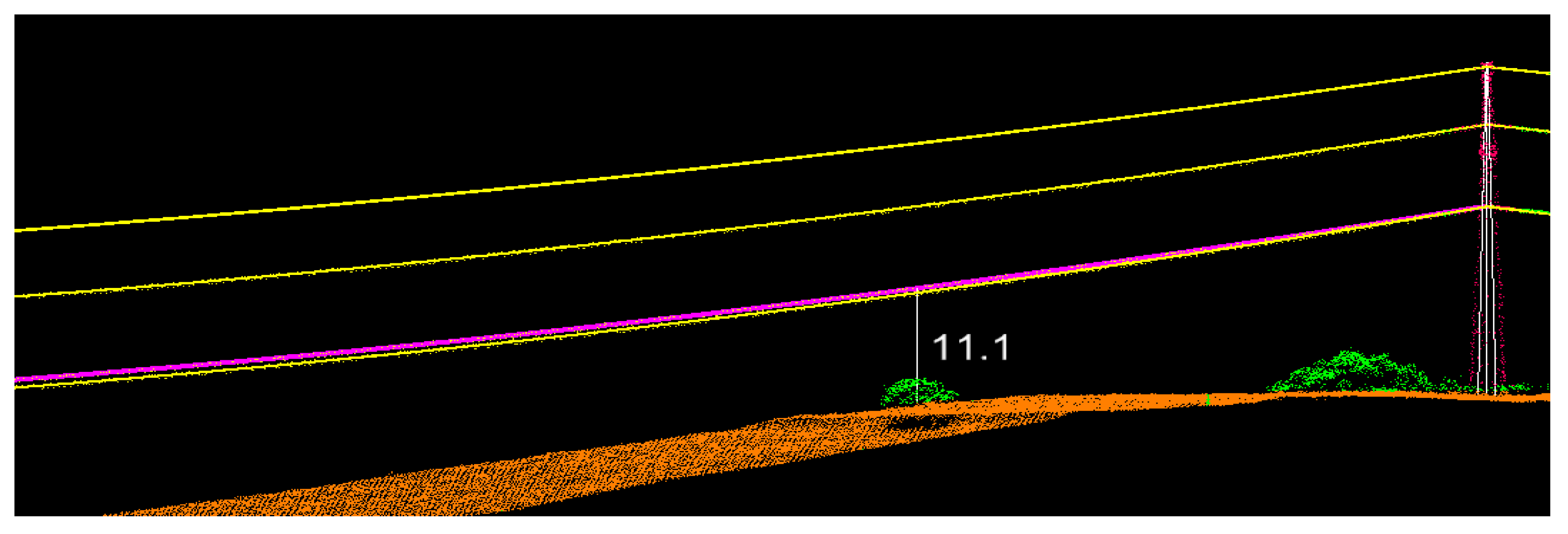
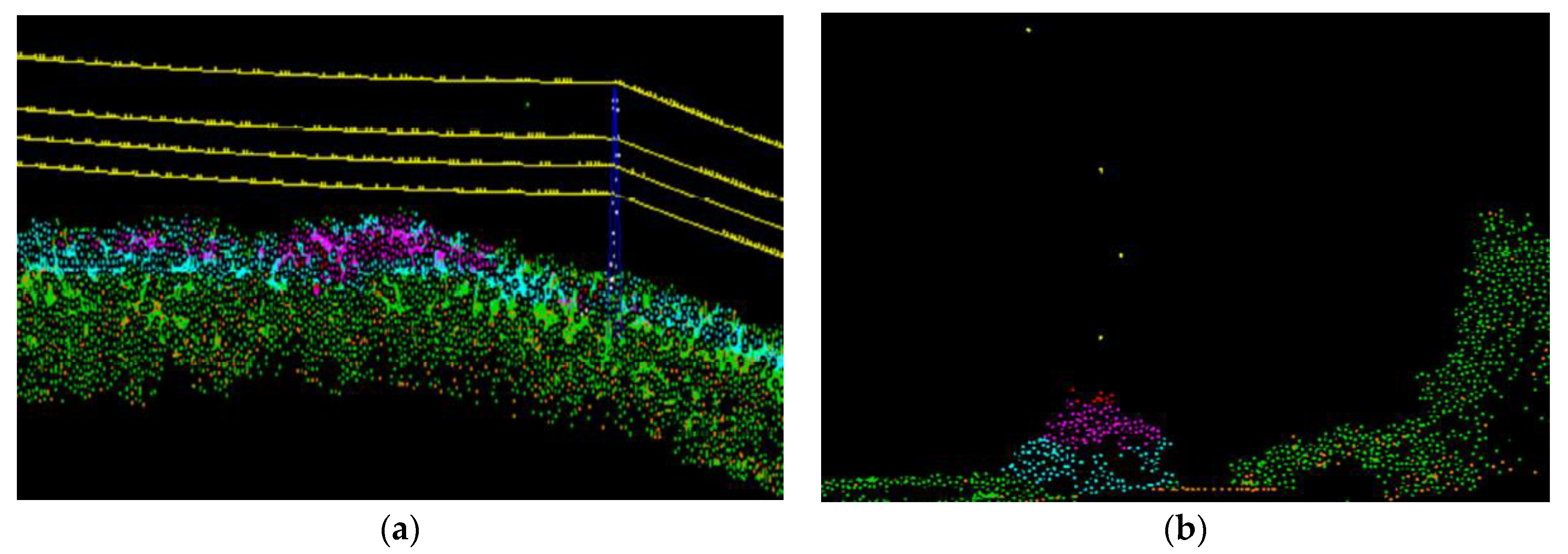
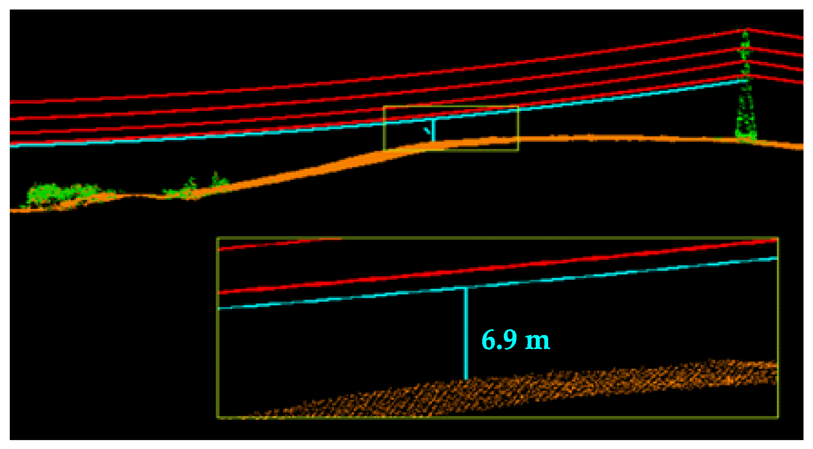
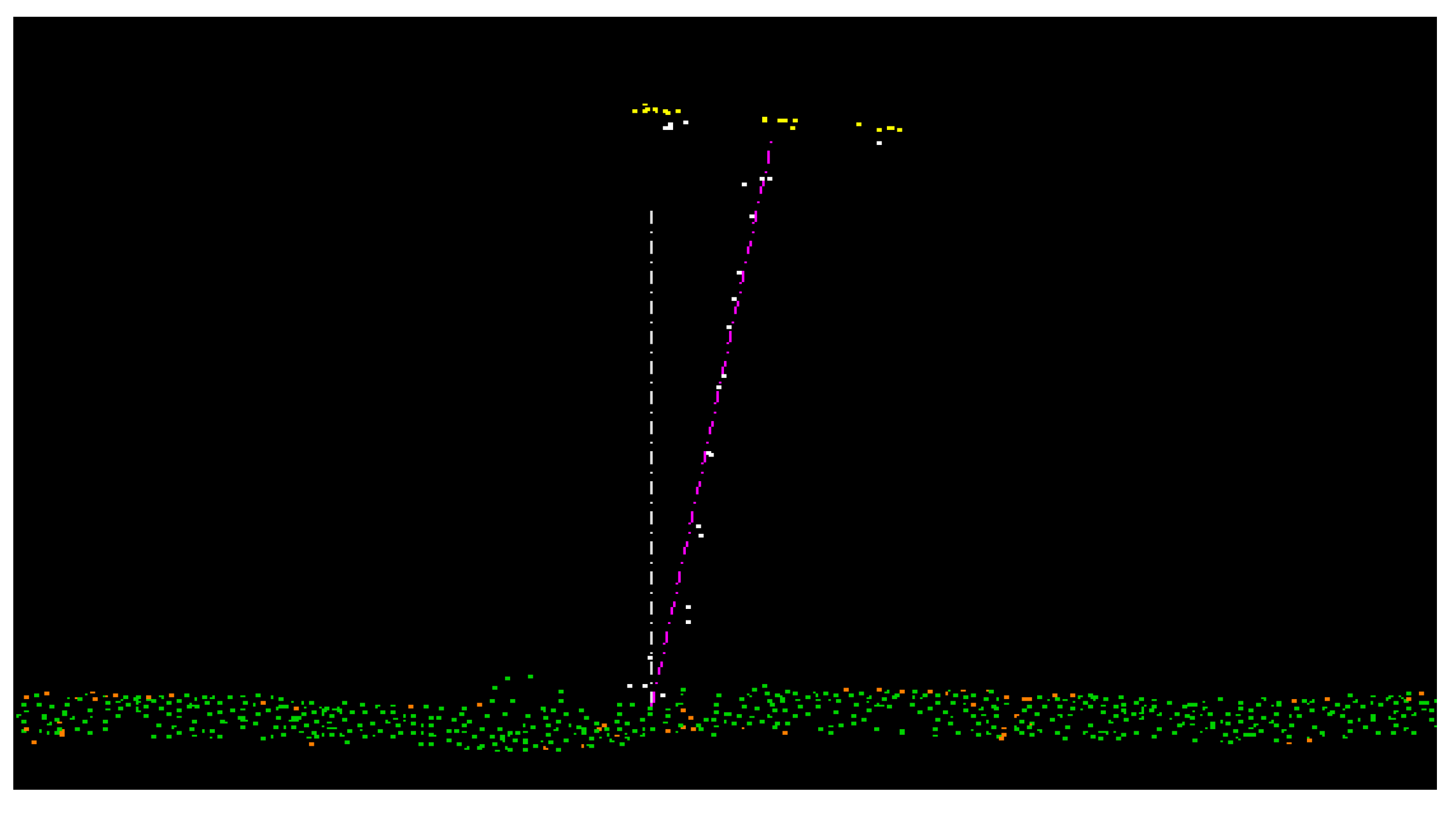
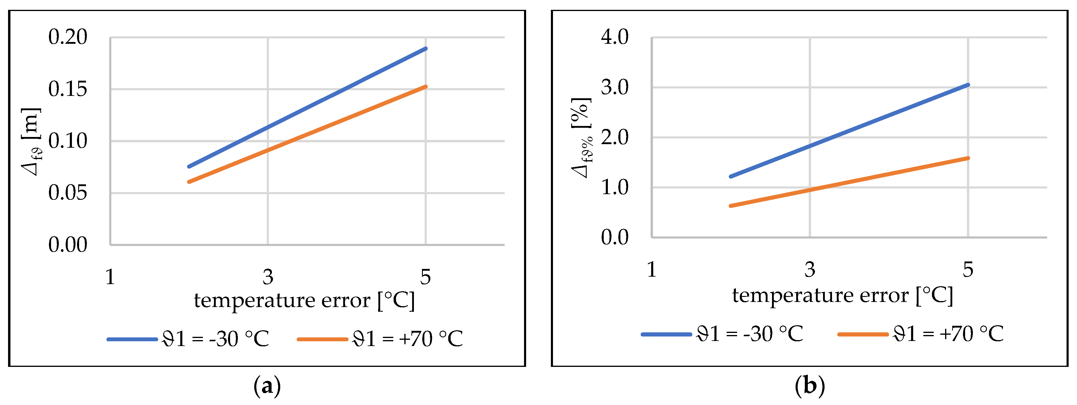
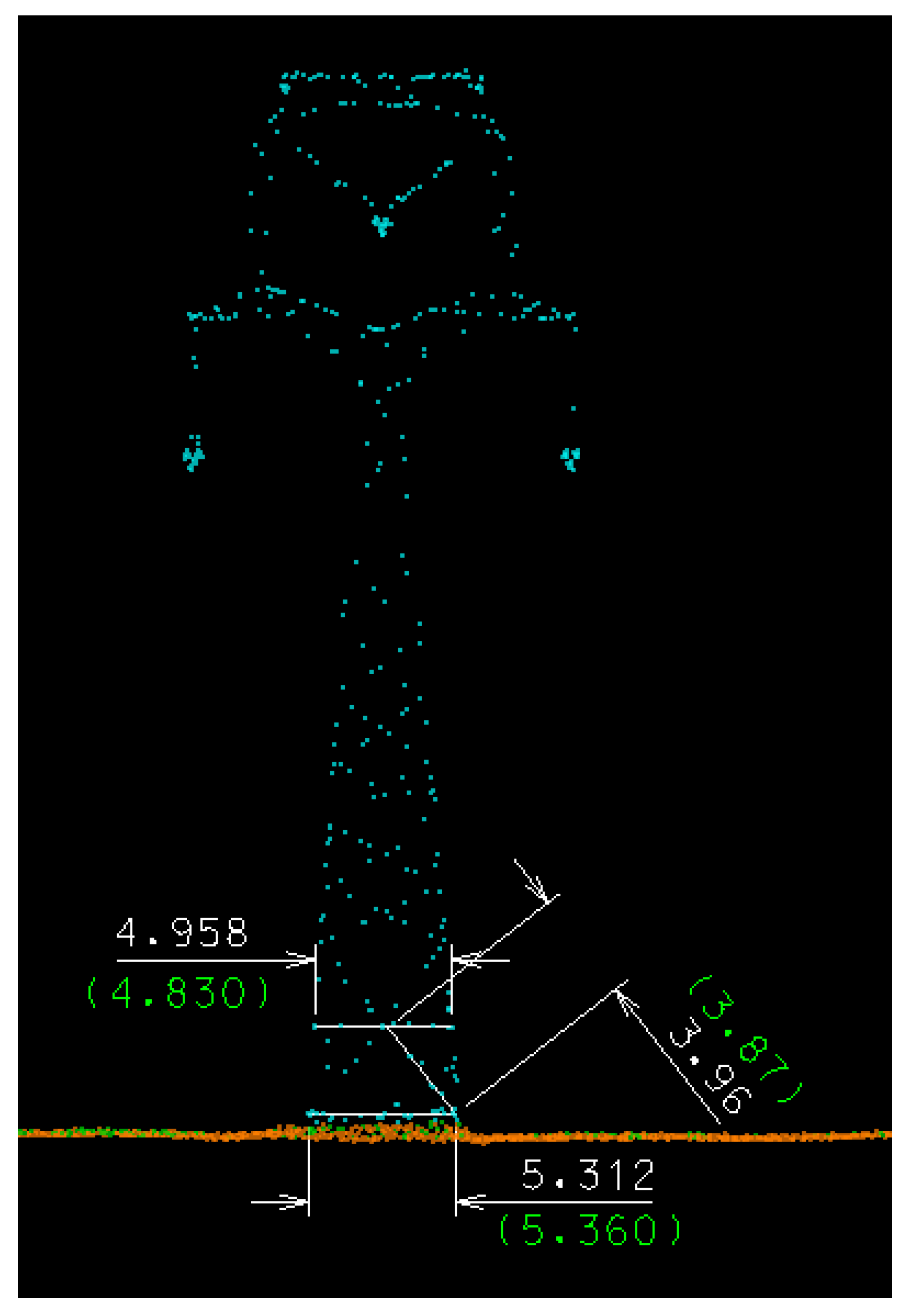
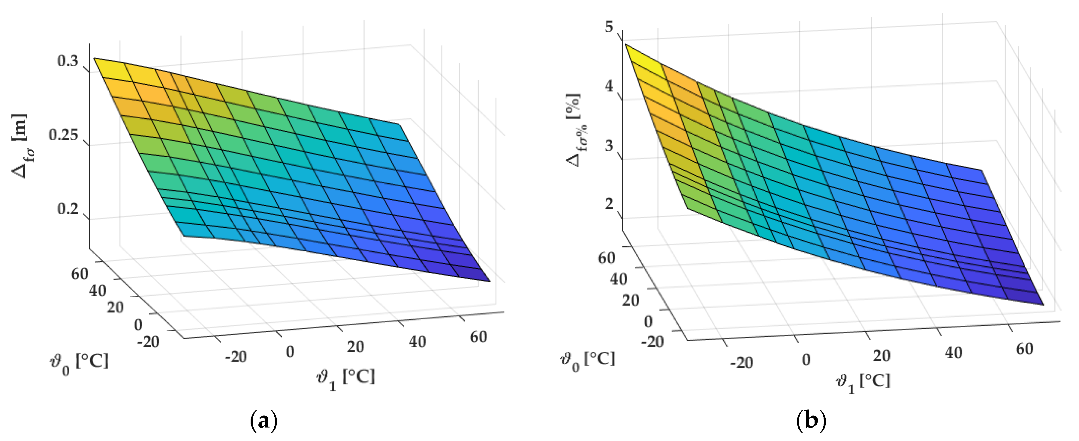
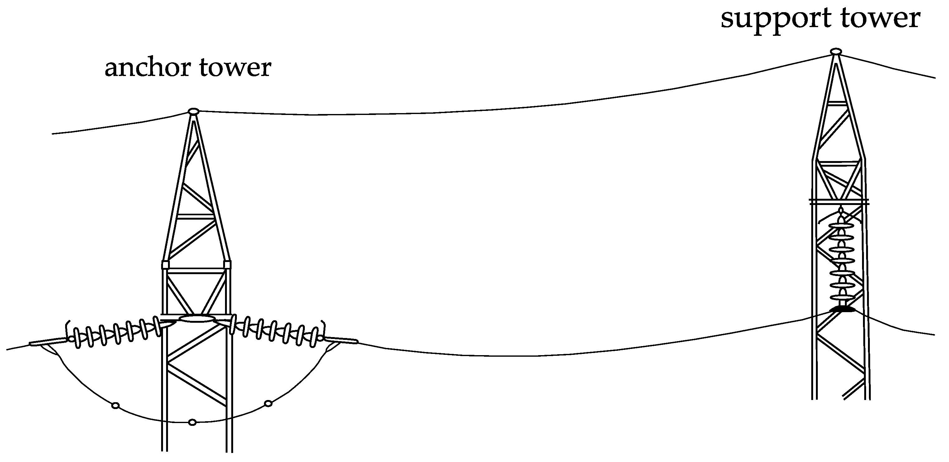
Table 1.
Mechanical parameters of the selected conductor ACSR 240/39.
| E [MPa] | [N×m−3] | α [°C−1] | [MPa] | d [mm] | q1 [N×m−1] | q2 [N×m−1] |
|---|---|---|---|---|---|---|
| 73,861 | 0.03427 × 10⁶ | 18.991 × 10⁻⁶ | 103.807 | 21.75 | 9.657 | 9.741 |
Table 2.
The reference sag-tension table of the ACSR 240/39 conductor, symmetrical tower span of 300 m, weak icing area N1.
Table 2.
The reference sag-tension table of the ACSR 240/39 conductor, symmetrical tower span of 300 m, weak icing area N1.
| ϑ1 [°C] | −30 | −20 | −10 | −5 | 0 | 10 |
| σH1 [MPa] | 62.199 | 58.651 | 55.535 | 54.118 | 52.785 | 50.345 |
| f [m] | 6.199 | 6.573 | 6.942 | 7.124 | 7.304 | 7.658 |
| ϑ1 [°C] | 20 | 30 | 40 | 50 | 60 | 70 |
| σH1 [MPa] | 48.170 | 46.220 | 44.464 | 42.873 | 41.426 | 40.104 |
| f [m] | 8.004 | 8.341 | 8.671 | 8.993 | 9.307 | 9.614 |
Note: mechanical tension of = 93.426 MPa and sag of f = 8.289 m correspond to the temperature −5 °C*.
Table 3.
Maximum absolute sag deviations Δfϑ caused by the incorrect determination of the initial conductor temperature by ±2 °C, ±3 °C, ±4 °C and ±5 °C.
Table 3.
Maximum absolute sag deviations Δfϑ caused by the incorrect determination of the initial conductor temperature by ±2 °C, ±3 °C, ±4 °C and ±5 °C.
| ϑ1 [°C] | −30 | −20 | −10 | −5 | 0 | 10 | 20 | 30 | 40 | 50 | 60 | 70 |
|---|---|---|---|---|---|---|---|---|---|---|---|---|
| Δfϑ ± 2 °C [m] | 0.076 | 0.075 | 0.073 | 0.072 | 0.072 | 0.070 | 0.069 | 0.067 | 0.065 | 0.064 | 0.062 | 0.061 |
| Δfϑ ± 3 °C [m] | 0.113 | 0.112 | 0.110 | 0.109 | 0.108 | 0.105 | 0.103 | 0.100 | 0.098 | 0.096 | 0.093 | 0.091 |
| Δfϑ ± 4 °C [m] | 0.151 | 0.149 | 0.147 | 0.145 | 0.144 | 0.141 | 0.137 | 0.134 | 0.131 | 0.128 | 0.125 | 0.122 |
| Δfϑ ± 5 °C [m] | 0.189 | 0.187 | 0.184 | 0.182 | 0.180 | 0.176 | 0.172 | 0.168 | 0.164 | 0.160 | 0.156 | 0.153 |
| fref [m] | 6.199 | 6.573 | 6.942 | 7.124 | 7.304 | 7.658 | 8.004 | 8.341 | 8.671 | 8.993 | 9.307 | 9.614 |
Table 4.
Comparison of bridge dimensions obtained from scanned point cloud and from real measurement.
Table 4.
Comparison of bridge dimensions obtained from scanned point cloud and from real measurement.
| Horizontal Accuracy | |||
| Analyzed Dimension | Scanned Value [m] | Measured Value [m] | Difference [cm] |
| Bridge width | 11.789 | 11.6 | 18.9 |
| Width of upper part of railing | 0.331 | 0.09 | 24.1 |
| Vertical Accuracy | |||
| Analyzed Dimension | Scanned Value [m] | Measured Value [m] | Difference [cm] |
| Railing height | 1.089 | 0.96 | 12.9 |
Table 5.
Maximum absolute sag deviations Δfσ [m] caused by the incorrect determination of the conductor initial mechanical tension.
Table 5.
Maximum absolute sag deviations Δfσ [m] caused by the incorrect determination of the conductor initial mechanical tension.
| ϑ1 | −30 | −20 | −10 | −5 | 0 | 10 | 20 | 30 | 40 | 50 | 60 | 70 | |
|---|---|---|---|---|---|---|---|---|---|---|---|---|---|
| ϑ0 | |||||||||||||
| −30 | - | 0.247 | 0.243 | 0.240 | 0.238 | 0.233 | 0.227 | 0.222 | 0.217 | 0.212 | 0.207 | 0.202 | |
| −20 | 0.254 | - | 0.246 | 0.243 | 0.241 | 0.236 | 0.230 | 0.225 | 0.219 | 0.214 | 0.209 | 0.204 | |
| −10 | 0.259 | 0.255 | - | 0.248 | 0.245 | 0.240 | 0.234 | 0.229 | 0.223 | 0.218 | 0.213 | 0.208 | |
| −5 | 0.262 | 0.258 | 0.253 | - | 0.247 | 0.242 | 0.236 | 0.231 | 0.225 | 0.220 | 0.215 | 0.210 | |
| 0 | 0.265 | 0.260 | 0.255 | 0.253 | - | 0.245 | 0.239 | 0.233 | 0.228 | 0.222 | 0.217 | 0.212 | |
| 10 | 0.271 | 0.266 | 0.261 | 0.259 | 0.256 | - | 0.244 | 0.238 | 0.233 | 0.227 | 0.222 | 0.217 | |
| 20 | 0.277 | 0.273 | 0.268 | 0.265 | 0.262 | 0.256 | - | 0.244 | 0.238 | 0.233 | 0.227 | 0.222 | |
| 30 | 0.284 | 0.280 | 0.274 | 0.271 | 0.268 | 0.262 | 0.256 | - | 0.244 | 0.238 | 0.233 | 0.227 | |
| 40 | 0.291 | 0.286 | 0.281 | 0.278 | 0.275 | 0.269 | 0.262 | 0.256 | - | 0.244 | 0.238 | 0.233 | |
| 50 | 0.298 | 0.293 | 0.288 | 0.285 | 0.282 | 0.275 | 0.269 | 0.262 | 0.256 | - | 0.244 | 0.239 | |
| 60 | 0.305 | 0.300 | 0.295 | 0.292 | 0.288 | 0.282 | 0.275 | 0.269 | 0.262 | 0.256 | - | 0.244 | |
| 70 | 0.312 | 0.307 | 0.302 | 0.298 | 0.295 | 0.288 | 0.282 | 0.275 | 0.268 | 0.262 | 0.256 | - | |
| fref [m] | 6.199 | 6.573 | 6.942 | 7.124 | 7.304 | 7.658 | 8.004 | 8.341 | 8.671 | 8.993 | 9.307 | 9.614 | |
Table 6.
Maximum absolute sag deviations ΔfE [m] caused by the incorrect determination of the conductor elasticity modulus by ±10%.
Table 6.
Maximum absolute sag deviations ΔfE [m] caused by the incorrect determination of the conductor elasticity modulus by ±10%.
| ϑ1 | −30 | −20 | −10 | −5 | 0 | 10 | 20 | 30 | 40 | 50 | 60 | 70 | |
|---|---|---|---|---|---|---|---|---|---|---|---|---|---|
| ϑ0 | |||||||||||||
| −30 | - | 0.010 | 0.019 | 0.023 | 0.026 | 0.032 | 0.037 | 0.042 | 0.045 | 0.048 | 0.051 | 0.053 | |
| −20 | 0.010 | - | 0.009 | 0.013 | 0.016 | 0.023 | 0.028 | 0.032 | 0.036 | 0.039 | 0.042 | 0.044 | |
| −10 | 0.019 | 0.009 | - | 0.004 | 0.008 | 0.014 | 0.020 | 0.024 | 0.028 | 0.032 | 0.034 | 0.037 | |
| −5 | 0.023 | 0.013 | 0.004 | - | 0.004 | 0.010 | 0.016 | 0.021 | 0.025 | 0.028 | 0.031 | 0.033 | |
| 0 | 0.027 | 0.017 | 0.008 | 0.004 | - | 0.007 | 0.012 | 0.017 | 0.021 | 0.025 | 0.028 | 0.030 | |
| 10 | 0.034 | 0.024 | 0.015 | 0.011 | 0.007 | - | 0.006 | 0.011 | 0.015 | 0.019 | 0.022 | 0.024 | |
| 20 | 0.041 | 0.030 | 0.021 | 0.017 | 0.013 | 0.006 | - | 0.005 | 0.009 | 0.013 | 0.016 | 0.019 | |
| 30 | 0.046 | 0.036 | 0.026 | 0.022 | 0.018 | 0.011 | 0.005 | - | 0.004 | 0.008 | 0.012 | 0.015 | |
| 40 | 0.051 | 0.041 | 0.031 | 0.027 | 0.023 | 0.016 | 0.010 | 0.005 | - | 0.004 | 0.007 | 0.010 | |
| 50 | 0.056 | 0.045 | 0.036 | 0.032 | 0.028 | 0.020 | 0.014 | 0.009 | 0.004 | - | 0.004 | 0.007 | |
| 60 | 0.060 | 0.049 | 0.040 | 0.036 | 0.032 | 0.024 | 0.018 | 0.012 | 0.008 | 0.004 | - | 0.003 | |
| 70 | 0.064 | 0.053 | 0.044 | 0.039 | 0.035 | 0.028 | 0.021 | 0.016 | 0.011 | 0.007 | 0.003 | - | |
| fref [m] | 6.199 | 6.573 | 6.942 | 7.124 | 7.304 | 7.658 | 8.004 | 8.341 | 8.671 | 8.993 | 9.307 | 9.614 | |
Table 7.
Maximum absolute sag deviations Δfγ [m] caused by the incorrect determination of the conductor specific gravity load by ±1%.
Table 7.
Maximum absolute sag deviations Δfγ [m] caused by the incorrect determination of the conductor specific gravity load by ±1%.
| ϑ1 | −30 | −20 | −10 | −5 | 0 | 10 | 20 | 30 | 40 | 50 | 60 | 70 | |
|---|---|---|---|---|---|---|---|---|---|---|---|---|---|
| ϑ0 | |||||||||||||
| −30 | - | 0.060 | 0.058 | 0.057 | 0.056 | 0.055 | 0.053 | 0.051 | 0.049 | 0.048 | 0.046 | 0.045 | |
| −20 | 0.068 | - | 0.064 | 0.063 | 0.062 | 0.060 | 0.058 | 0.056 | 0.054 | 0.053 | 0.051 | 0.050 | |
| 10 | 0.073 | 0.072 | - | 0.068 | 0.067 | 0.065 | 0.063 | 0.061 | 0.059 | 0.058 | 0.056 | 0.054 | |
| −5 | 0.077 | 0.074 | 0.072 | - | 0.070 | 0.068 | 0.066 | 0.064 | 0.062 | 0.060 | 0.058 | 0.057 | |
| 0 | 0.080 | 0.078 | 0.075 | 0.074 | - | 0.071 | 0.069 | 0.067 | 0.065 | 0.063 | 0.061 | 0.059 | |
| 10 | 0.086 | 0.084 | 0.081 | 0.080 | 0.079 | - | 0.074 | 0.072 | 0.070 | 0.068 | 0.066 | 0.064 | |
| 20 | 0.092 | 0.090 | 0.088 | 0.086 | 0.085 | 0.083 | - | 0.078 | 0.075 | 0.073 | 0.071 | 0.069 | |
| 30 | 0.099 | 0.096 | 0.094 | 0.093 | 0.091 | 0.089 | 0.086 | - | 0.081 | 0.079 | 0.077 | 0.075 | |
| 40 | 0.105 | 0.103 | 0.100 | 0.099 | 0.097 | 0.095 | 0.092 | 0.089 | - | 0.084 | 0.082 | 0.080 | |
| 50 | 0.112 | 0.110 | 0.107 | 0.105 | 0.104 | 0.101 | 0.098 | 0.095 | 0.092 | - | 0.088 | 0.085 | |
| 60 | 0.119 | 0.116 | 0.113 | 0.112 | 0.110 | 0.107 | 0.104 | 0.101 | 0.098 | 0.096 | - | 0.091 | |
| 70 | 0.126 | 0.123 | 0.120 | 0.118 | 0.117 | 0.114 | 0.110 | 0.107 | 0.104 | 0.101 | 0.099 | - | |
| fref [m] | 6.199 | 6.573 | 6.942 | 7.124 | 7.304 | 7.658 | 8.004 | 8.341 | 8.671 | 8.993 | 9.307 | 9.614 | |
Table 8.
Maximum absolute sag deviations Δfa [m] caused by the incorrect determination of the tower span by −2.5 m.
Table 8.
Maximum absolute sag deviations Δfa [m] caused by the incorrect determination of the tower span by −2.5 m.
| ϑ1 | −30 | −20 | −10 | −5 | 0 | 10 | 20 | 30 | 40 | 50 | 60 | 70 | |
|---|---|---|---|---|---|---|---|---|---|---|---|---|---|
| ϑ0 | |||||||||||||
| −30 | - | 0.105 | 0.107 | 0.108 | 0.108 | 0.110 | 0.111 | 0.112 | 0.114 | 0.115 | 0.117 | 0.118 | |
| −20 | 0.108 | - | 0.111 | 0.112 | 0.113 | 0.114 | 0.115 | 0.117 | 0.118 | 0.119 | 0.120 | 0.122 | |
| −10 | 0.113 | 0.115 | - | 0.117 | 0.117 | 0.119 | 0.120 | 0.121 | 0.122 | 0.123 | 0.125 | 0.126 | |
| −5 | 0.116 | 0.117 | 0.119 | - | 0.120 | 0.121 | 0.122 | 0.123 | 0.124 | 0.125 | 0.127 | 0.128 | |
| 0 | 0.119 | 0.120 | 0.121 | 0.122 | - | 0.123 | 0.124 | 0.125 | 0.127 | 0.128 | 0.129 | 0.130 | |
| 10 | 0.124 | 0.125 | 0.126 | 0.127 | 0.127 | - | 0.129 | 0.130 | 0.131 | 0.132 | 0.133 | 0.134 | |
| 20 | 0.129 | 0.130 | 0.131 | 0.132 | 0.132 | 0.133 | - | 0.135 | 0.136 | 0.137 | 0.137 | 0.138 | |
| 30 | 0.135 | 0.136 | 0.137 | 0.137 | 0.137 | 0.138 | 0.139 | - | 0.140 | 0.141 | 0.142 | 0.143 | |
| 40 | 0.140 | 0.141 | 0.142 | 0.142 | 0.143 | 0.143 | 0.144 | 0.144 | - | 0.146 | 0.146 | 0.147 | |
| 50 | 0.146 | 0.147 | 0.147 | 0.148 | 0.148 | 0.149 | 0.149 | 0.149 | 0.150 | - | 0.151 | 0.152 | |
| 60 | 0.151 | 0.152 | 0.153 | 0.153 | 0.153 | 0.154 | 0.154 | 0.154 | 0.155 | 0.155 | - | 0.156 | |
| 70 | 0.157 | 0.158 | 0.158 | 0.159 | 0.159 | 0.159 | 0.159 | 0.160 | 0.160 | 0.160 | 0.160 | - | |
| fref [m] | 6.199 | 6.573 | 6.942 | 7.124 | 7.304 | 7.658 | 8.004 | 8.341 | 8.671 | 8.993 | 9.307 | 9.614 | |
Table 9.
Final conductor sag uncertainties [m] caused by the cumulation of uncertainties of state equation input parameters. Temperatures , are in °C.
Table 9.
Final conductor sag uncertainties [m] caused by the cumulation of uncertainties of state equation input parameters. Temperatures , are in °C.
| ϑ1 | −30 | −20 | −10 | −5 | 0 | 10 | 20 | 30 | 40 | 50 | 60 | 70 | |
|---|---|---|---|---|---|---|---|---|---|---|---|---|---|
| ϑ0 | |||||||||||||
| −30 | - | 0.725 | 0.733 | 0.737 | 0.741 | 0.748 | 0.754 | 0.761 | 0.767 | 0.774 | 0.780 | 0.786 | |
| −20 | 0.670 | - | 0.691 | 0.696 | 0.700 | 0.708 | 0.716 | 0.723 | 0.731 | 0.738 | 0.745 | 0.752 | |
| −10 | 0.626 | 0.640 | - | 0.657 | 0.662 | 0.672 | 0.681 | 0.689 | 0.697 | 0.705 | 0.713 | 0.721 | |
| −5 | 0.605 | 0.620 | 0.633 | - | 0.645 | 0.655 | 0.665 | 0.673 | 0.682 | 0.690 | 0.698 | 0.706 | |
| 0 | 0.585 | 0.601 | 0.615 | 0.622 | - | 0.639 | 0.649 | 0.658 | 0.667 | 0.676 | 0.684 | 0.692 | |
| 10 | 0.544 | 0.563 | 0.580 | 0.587 | 0.594 | - | 0.618 | 0.629 | 0.639 | 0.648 | 0.657 | 0.666 | |
| 20 | 0.503 | 0.526 | 0.545 | 0.554 | 0.562 | 0.576 | - | 0.601 | 0.612 | 0.622 | 0.632 | 0.642 | |
| 30 | 0.462 | 0.488 | 0.510 | 0.520 | 0.529 | 0.546 | 0.561 | - | 0.586 | 0.598 | 0.608 | 0.618 | |
| 40 | 0.420 | 0.449 | 0.474 | 0.486 | 0.496 | 0.516 | 0.533 | 0.548 | - | 0.574 | 0.585 | 0.596 | |
| 50 | 0.379 | 0.409 | 0.437 | 0.450 | 0.462 | 0.484 | 0.504 | 0.521 | 0.536 | - | 0.562 | 0.574 | |
| 60 | 0.338 | 0.370 | 0.399 | 0.414 | 0.427 | 0.452 | 0.474 | 0.493 | 0.510 | 0.526 | - | 0.552 | |
| 70 | 0.300 | 0.331 | 0.361 | 0.376 | 0.391 | 0.418 | 0.443 | 0.464 | 0.484 | 0.501 | 0.516 | - | |
| fref [m] | 6.199 | 6.573 | 6.942 | 7.124 | 7.304 | 7.658 | 8.004 | 8.341 | 8.671 | 8.993 | 9.307 | 9.614 | |
Table 10.
Summary of results from Section 4.
Table 10.
Summary of results from Section 4.
| Parameter | Symbol | Uncertainty | Sag Deviation Δf [cm] |
|---|---|---|---|
| initial temperature | ±2–±5 °C | 6.1–18.9 | |
| point cloud accuracy 1 | - | ±25 cm | 20.2–31.2 |
| modulus of elasticity | ±10% | 0.3–6.4 | |
| specific gravity load | ±1% | 4.5–12.6 | |
| tower span | −2.5 m | 10.5–16.0 | |
| combination | - | according to 2 | 30–78.6 |
1 Affects the estimation of the initial mechanical tension . 2 = +5 °C, = −25 cm, = +10%, = −1%, = −2.5 m.
Publisher’s Note: MDPI stays neutral with regard to jurisdictional claims in published maps and institutional affiliations. |
© 2021 by the authors. Licensee MDPI, Basel, Switzerland. This article is an open access article distributed under the terms and conditions of the Creative Commons Attribution (CC BY) license (https://creativecommons.org/licenses/by/4.0/).
Share and Cite
MDPI and ACS Style
Siranec, M.; Höger, M.; Otcenasova, A. Advanced Power Line Diagnostics Using Point Cloud Data—Possible Applications and Limits. Remote Sens. 2021, 13, 1880. https://0-doi-org.brum.beds.ac.uk/10.3390/rs13101880
AMA Style
Siranec M, Höger M, Otcenasova A. Advanced Power Line Diagnostics Using Point Cloud Data—Possible Applications and Limits. Remote Sensing. 2021; 13(10):1880. https://0-doi-org.brum.beds.ac.uk/10.3390/rs13101880
Chicago/Turabian StyleSiranec, Marek, Marek Höger, and Alena Otcenasova. 2021. "Advanced Power Line Diagnostics Using Point Cloud Data—Possible Applications and Limits" Remote Sensing 13, no. 10: 1880. https://0-doi-org.brum.beds.ac.uk/10.3390/rs13101880
Note that from the first issue of 2016, this journal uses article numbers instead of page numbers. See further details here.