
A Multi-Branch Feature Fusion Strategy Based on an Attention Mechanism for Remote Sensing Image Scene Classification

1
College of Communication and Electronic Engineering, Qiqihar University, Qiqihar 161000, China
2
College of Information and Communication Engineering, Dalian Nationalities University, Dalian 116000, China
*
Author to whom correspondence should be addressed.
Remote Sens. 2021, 13(10), 1950; https://0-doi-org.brum.beds.ac.uk/10.3390/rs13101950
Submission received: 12 April 2021
/
Revised: 8 May 2021
/
Accepted: 11 May 2021
/
Published: 17 May 2021
(This article belongs to the Special Issue Feature-Based Methods for Remote Sensing Image Classification)
Abstract
:In recent years, with the rapid development of computer vision, increasing attention has been paid to remote sensing image scene classification. To improve the classification performance, many studies have increased the depth of convolutional neural networks (CNNs) and expanded the width of the network to extract more deep features, thereby increasing the complexity of the model. To solve this problem, in this paper, we propose a lightweight convolutional neural network based on attention-oriented multi-branch feature fusion (AMB-CNN) for remote sensing image scene classification. Firstly, we propose two convolution combination modules for feature extraction, through which the deep features of images can be fully extracted with multi convolution cooperation. Then, the weights of the feature are calculated, and the extracted deep features are sent to the attention mechanism for further feature extraction. Next, all of the extracted features are fused by multiple branches. Finally, depth separable convolution and asymmetric convolution are implemented to greatly reduce the number of parameters. The experimental results show that, compared with some state-of-the-art methods, the proposed method still has a great advantage in classification accuracy with very few parameters.
1. Introduction
Remote sensing image scene classification refers to the use of aerial scanning, microwave radar, and other methods to image the target scene and then extract useful information from different scene images, thus enabling an analysis and evaluation of the scene image. Relevant research on remote sensing scene classification has been widely used in national defense security [1], analyses of crop growth [2], and environmental management [3]. Because of the large content differences in the same scene, the similar content in different scenes, the inconsistent spatial scales of landforms, and the different shapes and sizes of images, remote sensing image scene classification has become a very challenging task. Therefore, in recent years, some researchers have focused on the effective scene classification of remote sensing images.
Deep learning, a very effective technology in the field of computer vision, was considered one of the ten technological breakthroughs in 2013. With the development of imaging technology and hardware equipment, deep learning has become widely used in remote sensing image scene classification and has natural advantages. Convolution neural networks (CNNs) can extract rich feature details from images and are used by most researchers [4,5,6]. However, increasingly, researchers are expanding the depths and widths of the neural networks to improve the performance of image classification. Although CNN has a certain role, the demand for computing equipment continues to increase, as does the necessary calculation time of the model.
Remote sensing image scene classification is a challenging task. In the early days, some traditional manual feature extraction methods and middle-level feature extraction methods were used. Researchers usually extracted the spectral, textural, and structural information of remote sensing images directly based on traditional methods, such as scale-invariant feature transform [7] (SIFT), generalized search trees [8] (GIST), and histogram of oriented gradients [9] (HOG). However, these methods are not very efficient. Then, some methods were proposed based on unsupervised learning methods, such as K-means clustering and Gaussian mixed models [10], sparse coding [11], and self-coding algorithms [12]. However, the extracted features are not ideal. Recently, feature extraction methods based on convolutional neural network have constantly been emerging. The earliest convolution neural network, LeNet, was proposed by Y. Lecun [13], and has been used in handwritten number recognition tasks. Krizhevsky and Hinton [14] suggested that AlexNet, which uses two GPUs that interact with each other, greatly improves the efficiency of training, which has aroused the interest of many researchers. Simonyan and Zisserman et al. [15] proposed VGGNet, which achieved a good classification accuracy via the linear stacking of multiple convolutions. Later, K. He proposed ResNet [16] by applying the idea of residual learning, adding jump links to the feature extraction network, and alleviating the problem of information loss in traditional convolution neural network layer transfer. Since then, most researchers have used these classical convolutional neural network models to improve the performance of remote sensing image scene classification. In addition, how to fuse each convolution layer to extract features is also a major factor to improve the model classification performance. The low-level feature image passes through less convolution layers, so it usually has lower semantics and more noise, which affects the classification performance of the model to some extent. According to this, feature fusion methods can be divided into the following two types: early fusion and late fusion. The former first fuses the extracted multi-layer features, and then trains the predictor with the fused features. The latter predicts multiple features, and then the prediction results are merged. Y. Liu et al. [17] found that there was considerable information in the shallow layer of the image. Therefore, a two-stage depth feature fusion model was proposed. This model integrates the two-stage features adaptively and further improves the performance of the model. However, it is still not a good solution to the problem of large intra-class differences and high inter-class similarity of remote sensing scene images. Then, Chaib [18], G. Cheng [19], and F. Zhao [20] proposed the discriminant correlation analysis (DCA) feature fusion method, the discriminative CNNs (D-CNNs) model, and variable-weighted multi-feature fusing (VWMF) model to solve these problems. However, in the D-CNN method of VGG16, the parameters of this method reached 130MB, which not only consumes a lot of training time, but also requires a high performance of computing environment.
Although the above network models can provide a good classification performance, the depth and complexity of networks are increasing. In 2016, a lightweight network (SqueezeNet) [21] was proposed, and the complexity of network gradually became the focus of attention. Then, in 2017, MobileNet [22] emerged and became popular because of its small network parameters and fast computational speed. Since then, it has become a research direction of many researchers for exploring a lightweight convolutional neural network with a small number of parameters and a high efficiency. Later, G. Cheng et al. [19] improved AlexNet and combined it with the D-CNN method. Compared with VGG16 as the basic network, the number of parameters is not only smaller, but the classification accuracy has also been improved to a certain extent. Y. Liu [17] proposed a two-branch model with a fixed scale and a different scale network that used AlexNet as the base model. Although the number of parameters for these methods has decreased somewhat, it still reaches up to 60 MB. Liu et al. proposed a weighted spatial pyramid matching collaborative-representation-based classification method, and further improved AlexNet, which is used as the basic network for feature extraction. W. Zhang et al. [23] proposed a capsule network structure based on InceptionNet, which focuses on the connection of spatial information while building a lightweight network, and reduces the information visibility loss. Although these methods can provide good classification accuracy, the number of parameters is still large, so the efficiency of the model is limited. Therefore, how to reduce the complexity of the model as much as possible while ensuring the classification accuracy is a problem that needs to be further studied. At the same time, the attention-based strategy has become a favorable method to improve the accuracy of classification.
In the field of artificial intelligence today, attention mechanisms are increasingly expected to focus on the details and locations of useful information, search for the important characteristics of the target, and filter out irrelevant information so as to improve the confidence of prediction. Attention mechanisms have emerged from research on human vision and perform well in many tasks, such as target detection [24], sentence generation [25], and speech recognition [26]. Attention mechanism is mainly divided into three categories, namely: soft attention, hard attention, and self attention. The soft attention mechanism model is differentiable. By extracting the correlation weights between different layers, it focuses on the correlation between the input features and target features. The hard attention mechanism model is non-differentiable. Reinforcement learning is usually used to explore the correlation between the input mechanism and the target extracted by the convolutional neural network, which is more difficult to train than the soft attention mechanism. The self attention mechanism mainly reflects the mutual attention of the input information, and processes the feature information extracted by different layers in parallel. In 2018, X. He et al. [27] proposed a sequence to sequence model that generates a question-and-answer dialogue language model by applying an encoder–decoder structure to multilingual translation. In addition, in 2017, a self-attention mechanism was proposed in [28], which alleviated the shortcomings of traditional attention mechanisms, which depend on external information and make greater use of the internal relationship of data. In 2019, Wang et al. [29] proposed a cyclic attention model. Since then, many researchers have tried to apply various attention mechanisms to remote sensing image scene classification according to the characteristics of dense connection between the layers of DenseNet and ResNet. W. Tong et al. [30] improved the DenseNet network and integrated it into a channel attention model. Then, the attention mechanism was used to enhance the weight of important feature information. D. Yu et al. [31] proposed a feature fusion framework based on hierarchical attention and bilinear pool (HABFNet) with ResNet50 as the basic network. The extracted information was enhanced and linearly fused. Through a large number of experiments, H. Alhichri et al. [32] found the location for integrating the attention mechanism into the specific convolutional layer in the model, and proposed a deep attention convolutional neural network (CNN), which makes the channel automatically adjust the weight of the learning feature information when training CNN end-to-end by back propagation. However, not all attention mechanisms are universal, and attention strategies should to be designed according to the characteristics of the networks. It remains a challenging task to develop an effective attention mechanism and to apply it to remote sensing scene classification.
For remote sensing image scene classification, a lightweight attention-based multi-branch feature fusion CNN (AMB-CNN) is proposed. On the premise of enlarging the field of perception, the proposed model utilizes an alternating combination of different convolutions for extracting deep features. The extracted effective information is sent to the attention module to obtain new features, which are fused with the features from the previous branches. The proposed AMB-CNN model can provide good performance in remote sensing image scene classification with lower complexity.
The main contributions of this paper are as follows:
(1) Two convolution combination modules for feature extraction are proposed. These modules use the method of multi-convolution cooperation outside the module and multi-convolution alternately inside the module to enable the model to more fully determine the key information of the image and to exactly discriminate the scene.
(2) A strategy for fusing multi-branch features is explored. After extracting the feature information from multiple branches, the attention mechanism is utilized to extract the branch information again. Ultimately, the multi-segment features are fused.
(3) To solve the rapid growth of the network model parameters in recent years, a lightweight model with fewer parameters is constructed. Different convolutions are utilized to reduce the number of parameters of the network model. Meanwhile, the hard-swish activation function is adopted to enhance the nonlinear representation ability of the model.
The rest of this paper is as follows. The proposed attention-based multi branch feature fusion convolutional neural network (AMB-CNN) method is described in detail in Section 2. In Section 3, the experiment and analysis are carried out, and a comparison with the state-of-the-art methods is used to show the effectiveness of the proposed method. Section 4 gives the discussion. The last section is the conclusions.
2. Materials and Methods
2.1. The Structure of the Proposed Method
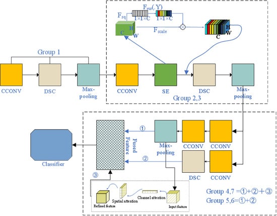
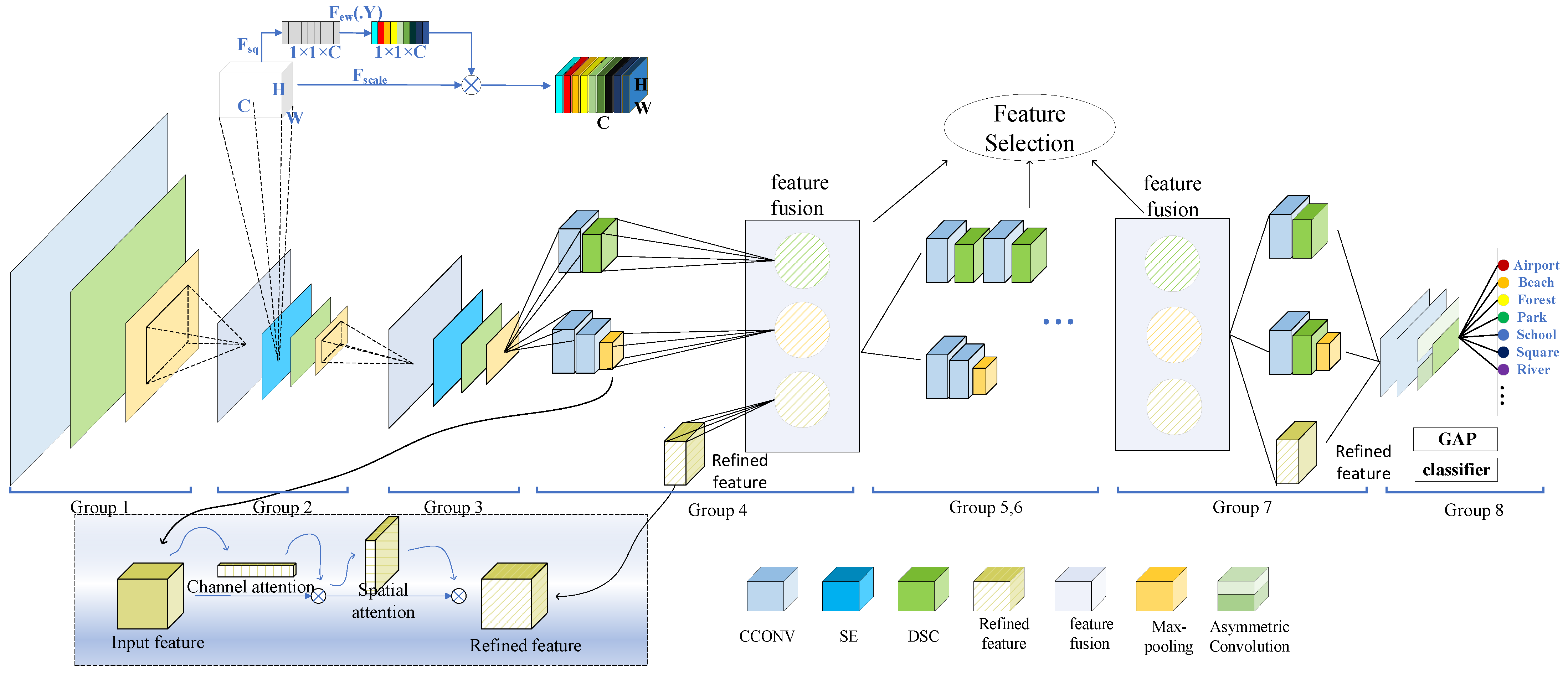
The AMB-CNN method consists of eight groups, as shown in Figure 1. Here, represents the compression process, represents the excitation process, is the channel feature after dimensionality reduction, is the height of the feature map, is the channel of the feature map, and represents the final output features of the squeeze and excitation modules. The first three groups are utilized to extract the shallow feature of the remote sensing images. This method combines the squeeze and excitation (SE) modules, enhances the relationship between feature channels, expands the global perception field, and reduces information loss during subsequent deep feature extraction. Starting with the fourth group, a multilinear fusion strategy based on spatial and channel attention is used to extract more useful information, as described in Section 2.2. Finally, in the eighth group, asymmetric convolution is added to further reduce the number of parameters. The process of the AMB-CNN model is described in Algorithm 1.
In the main part related to extracting deep features (groups 4 to 7), each group can be regarded as being composed of two modules whose inputs are obtained from the upper end. These two modules are the alternating combinations of ordinary and depthwise separable convolution, and a combination of ordinary and max-pooling layers, respectively. When the two modules are fused directly, although the extracted feature information is better than that of a single branch, the overall improvement effect is still not ideal. Therefore, the features extracted by one of the modules are input into the convolutional block attention module (CBAM). Then, the features are further extracted and multi-branch fusion is performed to obtain more key features, which is called , as described in the next section.
To build a lightweight network, this paper utilizes a combination of different convolutions to alleviate the problem of a large number of model parameters and to slow the training speed, and abandons the traditional method of the direct linear stacking of multiple large convolutions. Asymmetric convolution is applied in the eighth group of the model. Compared with traditional convolution, the parameter quantity is greatly reduced. A detailed introduction is provided in Section 2.3.
| Algorithm 1 Framework of the proposed AMB-CNN model |
| Input: is a feature map with size , the number of convolution kernels is |
| 1: Learn shallow features |
| 2: For in range Group 4 |
| 3: Extract the feature of target image |
| 4: Introducing dynamic features and activating channel weights |
| 5: Eliminate data offset ( represents the result after the normalization of the hidden layer, and represents the weight parameter and represents the input of any hidden layer activation function in the network) |
| 6: Mapping features to a high-dimensional, non-linear space end |
| 7: Learn deep features |
| 8: For in range (Group4:Group9) |
| 9: Through multi convolution cooperative feature exploration, are obtained ( represents the features of the second branch extracted from the fourth to seventh group) |
| 10: Generative attention characteristics ( is the global average pooling operations in spatial dimension, is the global max pooling operations in spatial dimension. is the global average pooling operations in channel dimension, is the global max pooling operations in channel dimension.) |
| 11: Fusion of multi segment features end |
| 12: classifier |
| 13: send to the classifier |
| Output: the predicted category labels |
As remote sensing scene images often have rich details and many landforms have a high similarity, the model has been adjusted slightly. A more stable hard-swish is used instead of ReLu as the activation function, which improves the non-linear representation ability of the model. Finally, the convergence speed of the model is accelerated via batch normalization (BN) layer processing. In addition, to prevent the phenomenon of over-fitting in training, an L2 regularization penalty is utilized. The details are described in Section 2.4.
2.2. Feature Extraction and Attention Module
The second and third groups of the model are designed to extract the shallow features of the image. Here, we add the SE module, which takes the upper convolution block as the input, uses the average pooling layer to compress each channel, and employs the dense layer to increase the nonlinearity so as to reduce the complexity of the output channel. Next, a dense layer is used to give the channel a smooth gating function. Finally, each feature map is weighted to expand the field of perception, reduce the loss of feature information, and provide more detailed information for the feature extraction from the fourth group. The SE module includes the following two parts: squeeze and excitation. A detailed explanation is provided in the following.
represents a set of filter kernels learned and represents the parameters of the filter. The output can be show as follows:
where represents the operation of convolution, is a feature map with size , represents the information of the -th output channel, and represents the convolution kernel used in channel of the input.
The channel correlation is reflected in the spatial correlation of the image, and now the two are combined. When extracting the channel information, global average pooling is used to compress multiple channels into one channel, where channel is
where is the height of the feature map and is the width of the feature map. To obtain the channel correlation, a gate function is employed, and a sigmoid is used as the activation function, as follows:
where is the activation function, is the output of the activation function, is the channel, and represents the weights of the fully connected layers used for the dimension reduction and dimension elevation. The gate mechanism is parameterized by forming a bottleneck around the nonlinearity of two fully connected (FC) layers—that is, the dimension-reducing layer parameter is , and the dimension-reducing scale is . By adjusting the output with the activation function, the final output of the attention module is
where refers to the corresponding channel product between the feature map and the original eigenvalue .
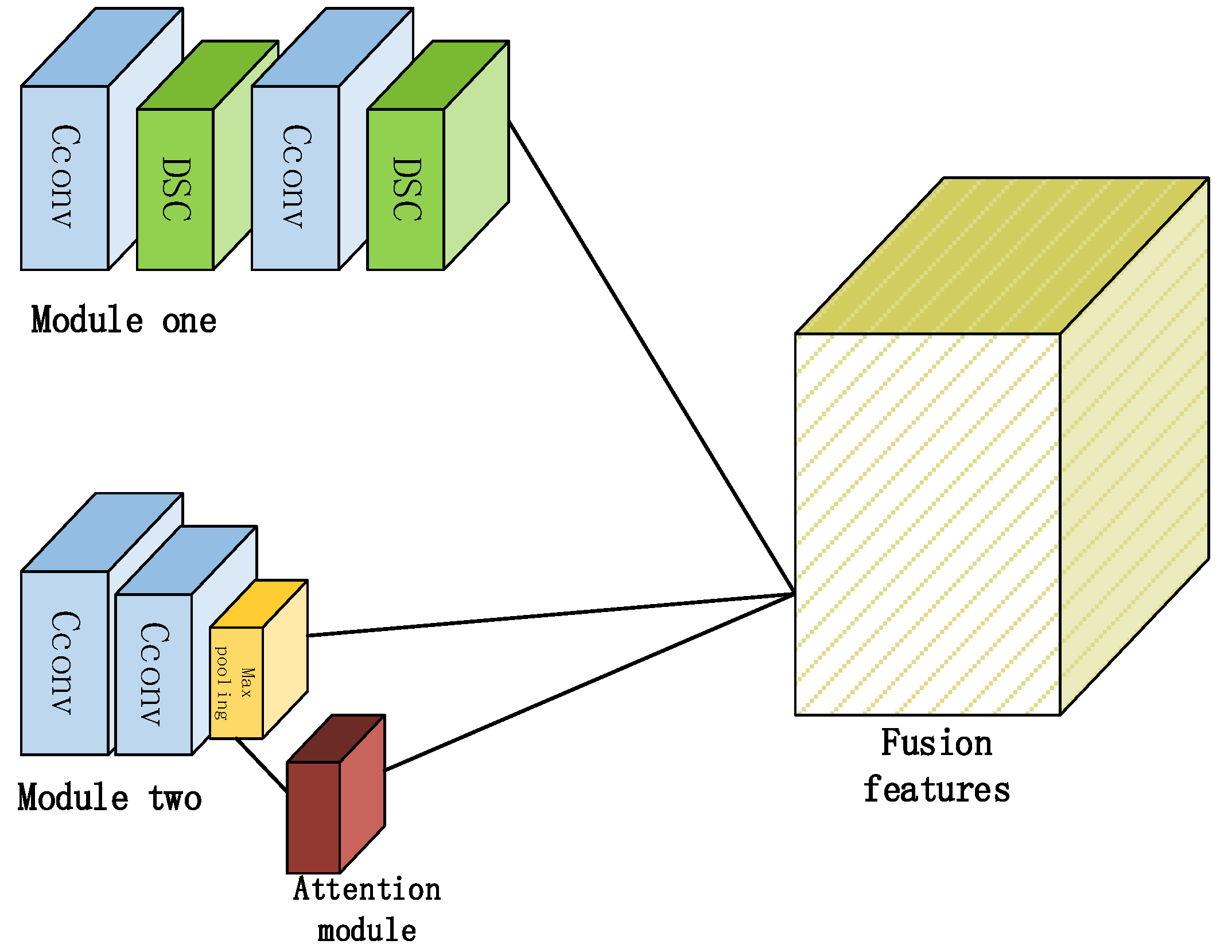
For the main part of the image feature extraction (Groups 4 to 7), two modules are proposed in this paper. The first module involves the alternate use of 2D convolution and depthwise separable convolution. In the second part, the 2D convolution and the max-pooling layer are cascaded, as shown in Figure 2.
On this basis, the channel and spatial attention mechanisms are added to the beginning layer (the fourth layer) and the end layer (the seventh layer) for deep feature extraction. It should be noted that the beginning layer refers to the beginning stage of extracting the deep features (groups 4 to 7 in the model), rather than the beginning of the whole model. The output feature map of the second module is transmitted to the convolutional attention module (CBAM). We input a one-dimensional feature map of CBAM as , with the dimensions of , and a two-dimensional feature map , with the dimensions of . Then, the degree of attention can be represented as follows
where represents the multiplication of elements, represents the output feature map of channel attention, and represents the final output feature map of the CBAM attention module. In this way, the key information and location of the feature map can be further obtained when the receptive field of the shallow features is enlarged. Furthermore, the ability of the feature extraction is enhanced.
2.3. Some Strategies of Building Lightweight Model
In the feature extraction, with the increase in the number of layers, the number of parameter calculations also increases. Taking a 3 × 3 convolution as an example, the parameter cost is massive after multi-channel convolution. Therefore, in the proposed model, a hybrid method of depthwise separable convolution combined with traditional 2D convolution is adopted, and the BN layer and nonlinear activation function are used after convolution to accelerate the convergence speed. The complexity and parameters of the depthwise separable convolution and the traditional 2D convolution are also compared.
Suppose the size of the input feature map is , the size of the output feature map is , and the size of the convolution kernel is . Then, the ordinary convolution parameter is . Depthwise separable convolution can be regarded as the sum of the pointwise convolution and depthwise separation convolution, where the parameter of the pointwise convolution is , and the parameter of the depthwise convolution is . The ratio of deep separable convolution to ordinary convolution can be represented as , which can be further represented as after simplification.
The number of parameters can be reduced by about nine times when using a 3 × 3 convolution kernel, and by about 25 times when using a 5 × 5 convolution kernel.
In order to measure the computational complexity, the convolution step is set to 1. As the zero-fill feature maps can ensure the same space size, the feature map of common convolution output is
The computational complexity is . Here, the complexity is related to the dimensions of the input and output channels, the input feature map, and the convolution kernel. The depthwise separable convolution used here does not depend on the size relationship between the convolution kernel size and the input feature map. In this paper, each channel is convoluted step by step, as follows:
where represents the channel of the output feature map, is the convolution kernel, is the height of the feature map, is the width of the feature map, is the number of convolutional kernels, is the length of convolutional kernel, is the number of channels, and is the step of the convolutional kernel.
In addition, in the eighth group of the proposed model, several asymmetric convolution fusion strategies are used to extract deeper features. Inspired by inception v3, by using multiple small convolution fusion instead of large convolution, we found that the cascade of 1 × 3 convolution and 3 × 1 convolution can reduce the convolution computation by about 33% compared with that using 3 × 3 directly. In this way, the computational complexity of the model can be reduced effectively without affecting the performance of the network model.
2.4. The Strategy of Nonlinear Feature Enhancement
The activation function plays an important role in training convolution neural network models. The traditional ReLu function is as follows:
Although this function converges faster than the Sigmoid function, ReLu is fragile during training. If parameters such as the learning rate are set inappropriately, when neuron necrosis occurs, the subsequent parameters will never be updated. The Sigmoid activation function can be represented as
The derivative of it is
In back propagation, when the gradient is close to 0, the weights are not updated, so the gradient can easily disappear. The hard-swish activation function is adopted in the proposed model and is characterized by smooth nonlinearity with no upper bound or lower bound. In training, although this function’s cost on embedded devices is non-zero, in general, the convolution layer/full connection layer of flops is the main computational model, which accounts for more than 95%, while the impact caused by the small cost of the hard-swish is negligible. After the convolution of each layer, the BN layer and activation function are added, which not only accelerates the training time of the model, but also enables the neurons to adapt more fully to complex, non-linear tasks. At the same time, the data offset can be eliminated to some extent, which can be seen in Algorithm 1.
During the model training stage, a type of weight attenuation, called L2 regularization, is added to make the representative data distribution stand out. For the proposed model, a regular term is added after the cost function:
and the partial derivative can be obtained to yield
The gradient descent is
when the coefficient of is 1, clearly, , which indicates that during the training process, the weight is attenuated, resulting in a smaller weight. Moreover, L2 regularization is adopted to alleviate the over-fitting phenomenon. In the experiment, the regularization coefficient of L2 is set to 0.005.
2.5. Dataset Settings
2.5.1. UC Merced Land-Use Dataset (UCM21)
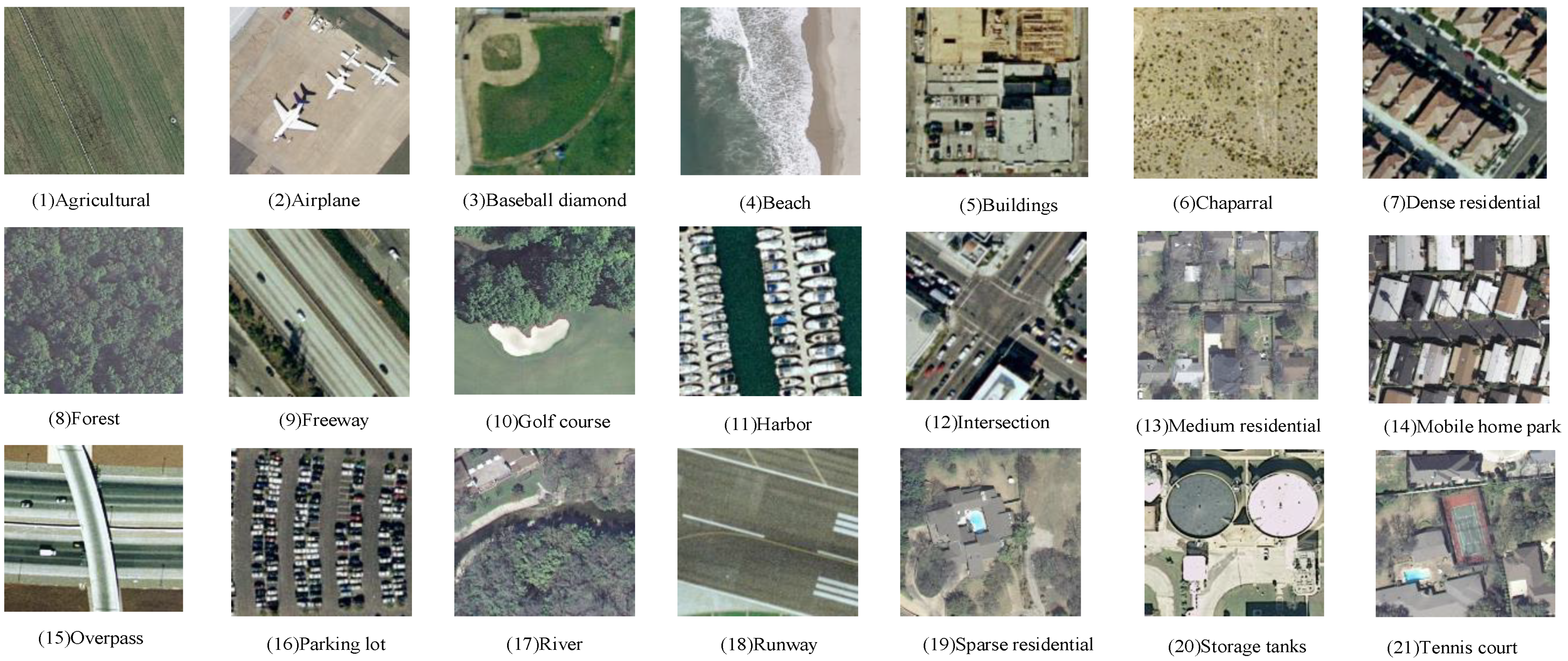
The images of this dataset are manually extracted from the USGS National Map Urban Area Image Set for urban areas across the country. The spatial resolution of the image is 0.3 m. For UCM 21 datasets, the image size is 256 × 256 and contains 21 types of scene images, 100 of each type, and 2100 spatial images. In the experiment, 80% randomly selected images from UCM 21 are used for the training. The remaining images are used for testing. Some scene images are shown in Figure 3.
2.5.2. AID30 Dataset
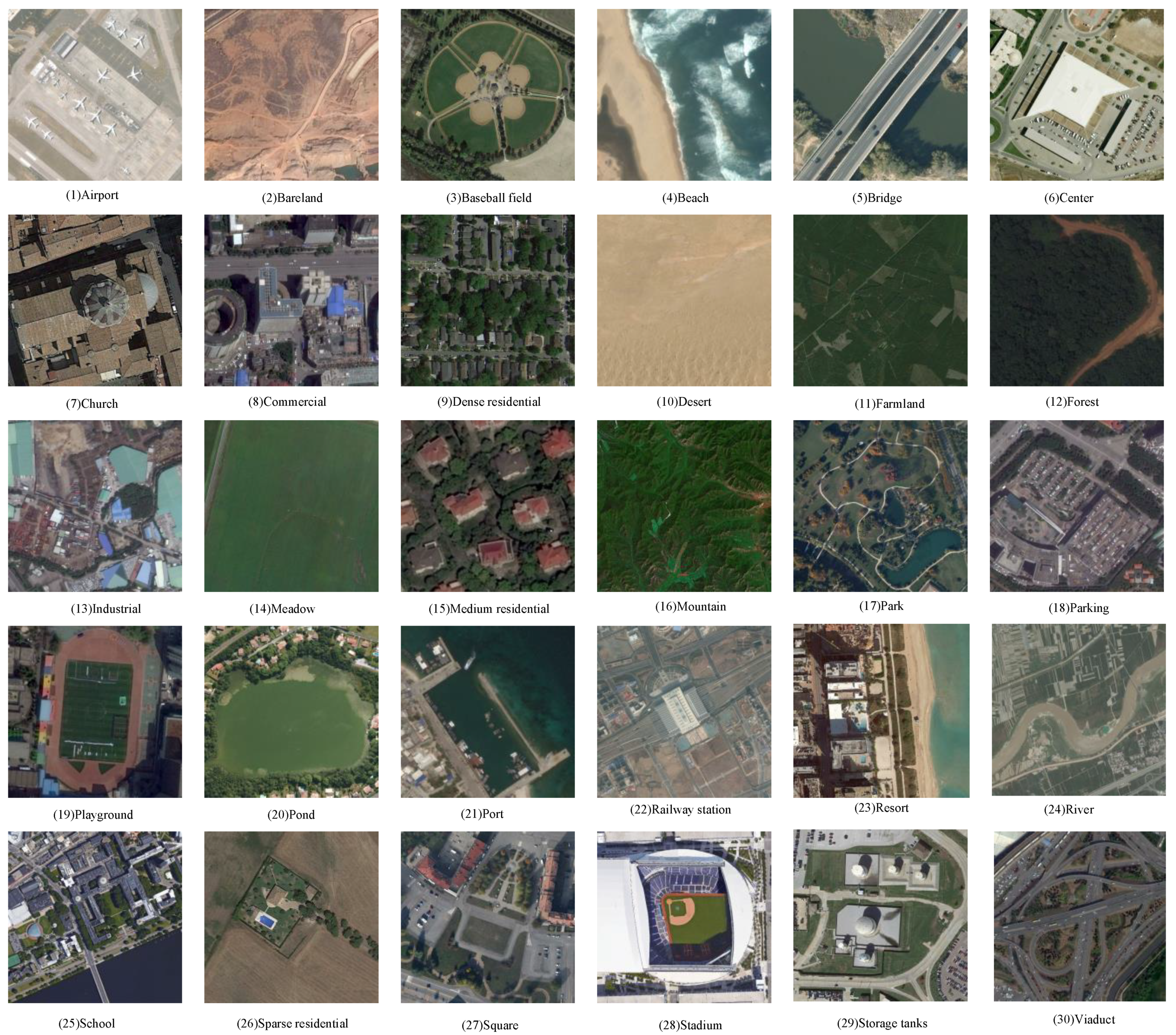
The AID30 dataset is obtained by collecting samples from Google Earth images, which is a large aerial image dataset. It comes from different remote imaging sensors, covering different seasons in China, the United States, Germany, France, the United Kingdom, Italy, and other countries. Therefore, it is a very challenging dataset. The spatial resolution of the image is 0.5–0.8 m. Compared with the UCM datasets, the AID30 datasets feature more images and categories with image sizes of 600 × 600, and a total of 30 categories of scene images, each of which contains about 220~420 images, totaling 10,000 images. Some scene images are shown in Figure 4.
To evaluate the proposed method effectively, two different data partitioning methods are employed.
(1) In the experiment, 20% of the images are randomly selected for training, and the rest are used for testing.
(2) In the experiment, 50% of the images are randomly selected for training, and the rest are used for testing.
2.5.3. RSSCN7 Dataset
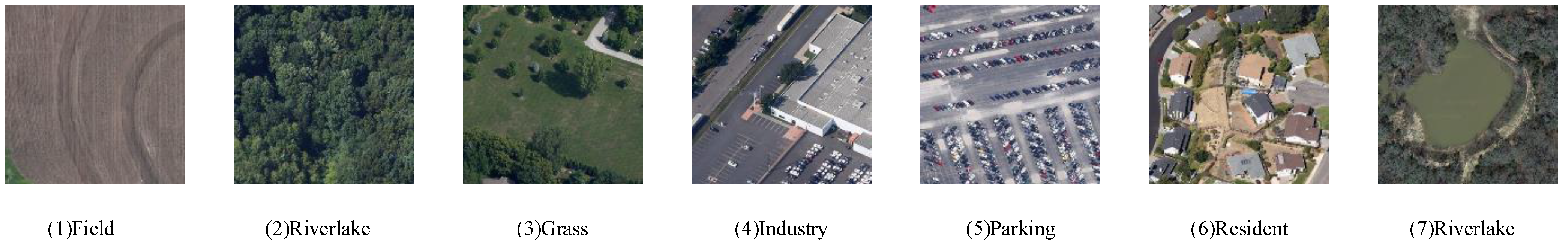
The RSSCN7 dataset was released by Qin Zou Yu of Wuhan University in 2015. These images are obtained in different seasons and weather changes, and are sampled with four different scales. The RSSCN7 dataset includes seven types of scene images, 400 × 400 in size. Each type is represented by 400 images, for a total of 2800 images. In the experiment, 50% of the images are randomly selected for training, and the rest are used for testing. Some scene images are shown in Figure 5.
2.5.4. NWPU45 Dataset
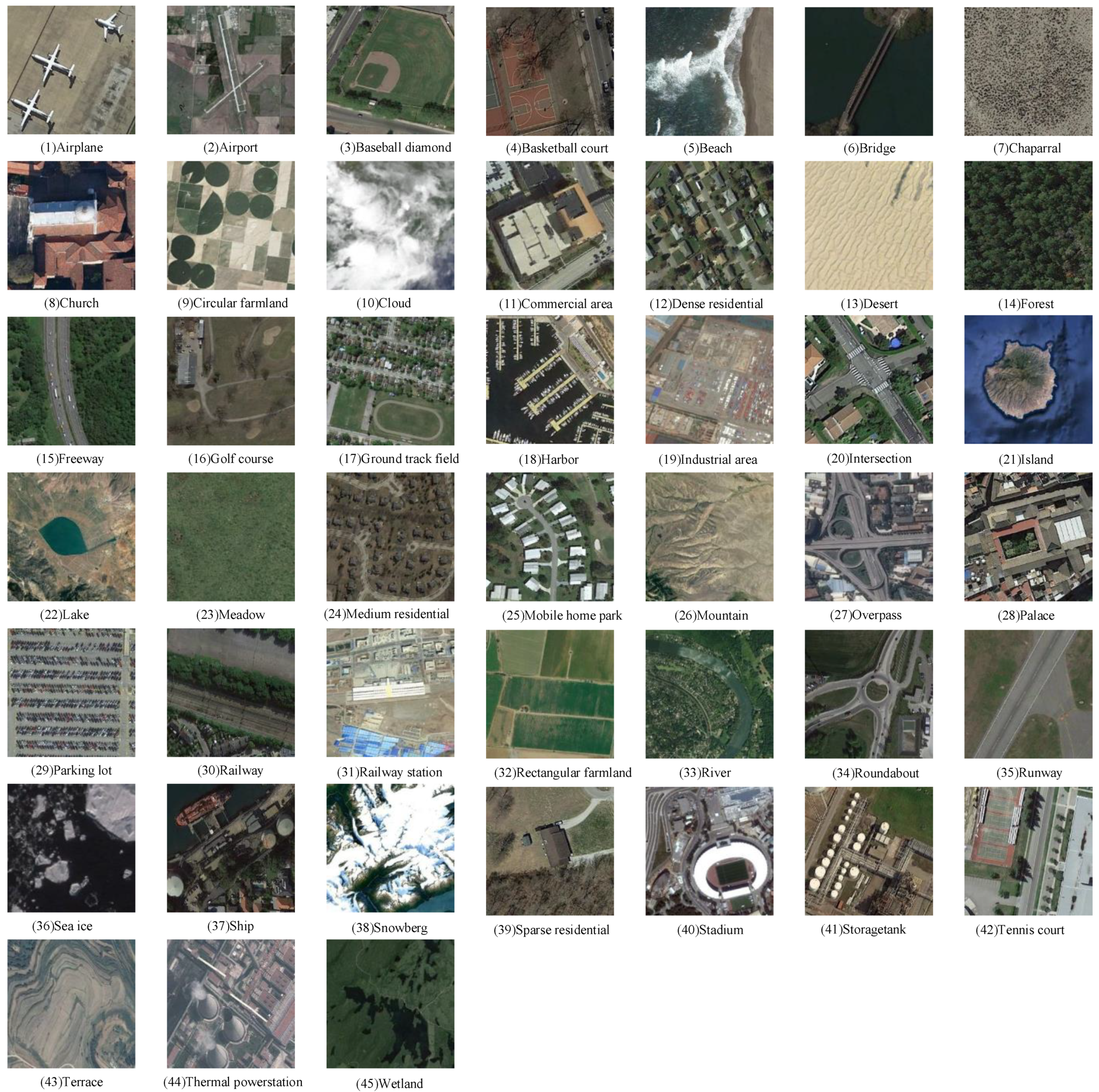
The NWPU45 dataset is large, covering more than 100 regions around the world. It is composed of images obtained by Google Earth through satellite images, aerial photography, and geographic information system (GIS). The images of the dataset selected for this study include different angles, lighting conditions, time, and seasons, so the similarity between classes is very high, which makes the process more challenging. The size of each image is 256 × 256, with 45 types of scene images, each of which is represented by 700 images, for a total of 31,500. The spatial resolution of the images is 0.2–30 m. Some scene images are shown in Figure 6. Two different data partition methods are used in the experiment.
(1) In the experiment, 10% of the images are randomly selected for training, and the rest are used for testing.
(2) In the experiment, 20% of the images are randomly selected for training, and the rest are used for testing.
(3) In the experiment, 80% of the images are randomly selected for training, and the rest are used for testing.
3. Experiment and Analysis
3.1. Setting of the Experiments
3.1.1. Data Preprocessing
A. Normalize the input image
B. Rotate the input image 0–60 degrees
C. Randomly flip the input image horizontally or vertically
D. Randomly offset the size of the image by 0.2 times
3.1.2. Parameter Settings
The initial learning rate is 0.01. The momentum of training is 0.9, and the batch size is set to 16. The experiments are conducted on a computer with an Intel (R) Core (TM) i7-10750H CPU, and RTX2060 GPU, and 16 GB of RAM.
3.2. The Performance of the Proposed Model
The proposed model is based on an improvement of the MobileNet network. To prove the effectiveness of an attention-based multi-branch fusion strategy in the model, firstly, the proposed model and MobileNet model are compared with the UCM21, AID30, NWPU45, and RSSCN7 datasets. The overall accuracy (OA), kappa coefficient, F1 coefficient, and average precision (AP) are adopted as the evaluation indexes. In the experiment, keras is adopted to reproduce MobileNet and to fine-tune the last layer of the network. Table 1 gives the comparison results of the OA, kappa coefficient, AP, and F1 score between the proposed model and the MobileNet model.
It can be seen from Table 1 that the classification performance of the proposed method is better than that of MobileNet. For the AID30 dataset, when the proportion of training sample and test sample is 20% and 80% (i.e., 20/80), respectively, the OA of the proposed method is 6.06% higher than that of MobileNet, and the kappa of the proposed method is higher by 6.28% than that of MobileNet. The F1 and AP results of the proposed method are also the highest. For other datasets with different proportions of training samples and test samples, the proposed method also shows an excellent classification performance. This proves that the proposed attention-based multi-branch fusion strategy can further extract the depth features of the remote sensing images, thus improving the classification performance of the remote sensing images.
In addition, on the UCM21 (20/80) dataset, the confusion matrix obtained by the proposed method and the MobileNet model are compared, as shown in Figure 7. It can be seen from Figure 7a that the proposed method provides a 100% correct classification rate for almost all of the categories. Moreover, the number of classification error samples is far less than that of the MobileNet model.
To summarize, by using multiple evaluation indicators (OA, AP, kappa, and F1 confusion matrix), the classification performance of the proposed method on six datasets is higher than that of MobileNet. This proves the effectiveness of multi-branch fusion strategy based on attention, which offers an excellent performance in remote sensing image scene classification.
3.3. Comparison with Advanced Methods
The proposed AMB-CNN method considers the feature information and location of the feature information comprehensively, applies the feature map with an enlarged receptive field to the two convolution model structures, extracts the feature, and finally fuses the multiple branches obtained through the attention mechanism. In this way, not only the classification accuracy is effectively improved, but the complexity of the model is also greatly reduced.
In the experiment, the proposed method is evaluated comprehensively through a comparison with some state-of-the-art methods under the same conditions. Firstly, some experiments are carried out on UCM21 dataset with training/test ratio of 8:2, the comparison results are shown in Table 2.
Here, the OA of the proposed model is 0.31% higher than that of the recently proposed PANet50 [48] model and 0.23% higher than that of the LCNN-BFF dual branch fusion network. Moreover, the parameters of the proposed model are only 5.6 M compared with the SF-CNN of VGGNet [47], VGG16-DF [46], and FACNN [44]. Taking VGG16 as the basic network model, the parameter amounts only account for 4.3% of these methods. For models based on ResNet, such as PANet50, the number of parameters is only 20%. Notably, the proposed AMB-CNN method still maintains the best performance with the fewest parameters. For a more comprehensive evaluation of the proposed method, the UCM21 dataset is used for the cross validation (five-fold) experiment, and the OA accuracy of the proposed AMB-CNN method is 99.49%.
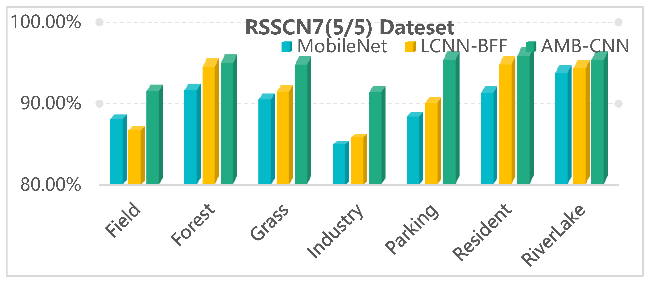
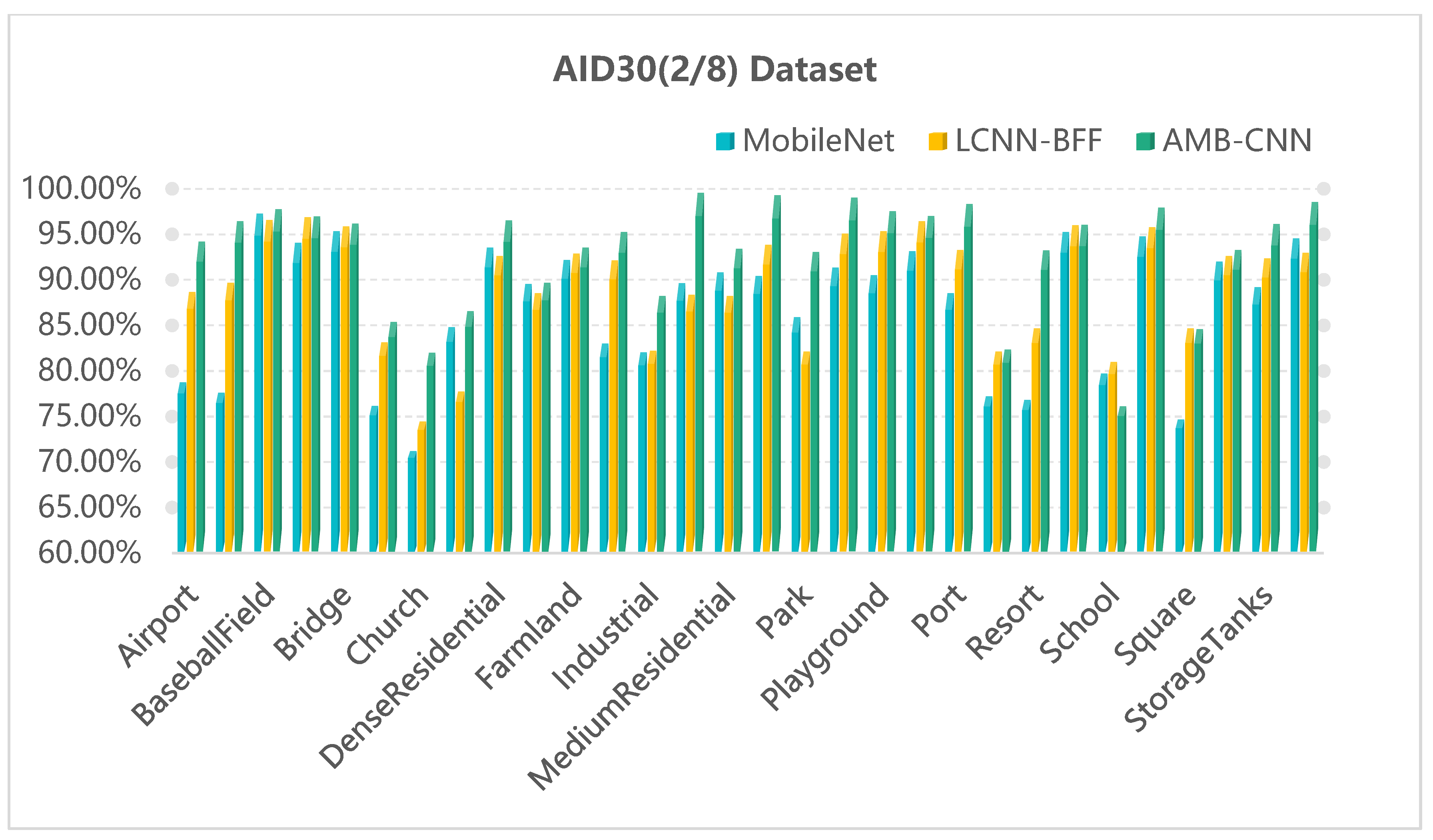
Figure 8, Figure 9 and Figure 10 show the AP comparison results of MobileNet, LCNN-BFF, and the proposed AMB-CNN method for the RSSCN7 (5/5), AID30 (2/8), and NWPU45 (1/9) datasets, respectively. The experiments show that the APs of the AMB-CNN method are higher than those of the other two methods for each specific category. These results illustrate that the strategy of multi-branch and attention fusion can extract the image feature more effectively and can reduce the loss of useful information, which enables this strategy to provide an excellent classification performance.
Next, some experiments are carried out on the RSSCN7 dataset with a training/test ratio of 5:5. The results are shown in Table 3. Here, the proposed model still has great advantages on the RSSCN7 datasets with a high similarity between classes. Compared with the two-stage deep feature fusion [17] method, the SPM-CRC [40] method, the WSPM-CRC [40] method, and the LCNN-BFF [49] method, the OA of the proposed method is improved by 2.77%, 1.28%, 1.24%, and 0.50%, respectively. Compared with the ADFF method, although the OA of the proposed method is slightly lower, the number of parameters is only 24.3% that of the ADFF method. In general, the complexity of the proposed network model is greatly reduced at the cost of a slight decrease in classification accuracy. In addition, in order to avoid biased results, a cross-validation (five-fold) experiment is also used on the RSSCN7 dataset. The OA accuracy of the proposed method reaches 96.07%, which proves the effectiveness of the proposed method.
Table 4 shows the experimental results on the AID dataset after a training/test ratio of 2:8 and training/test ratio of 5:5. In the AID30 (20/80) classification, the proposed method still provides the best classification accuracy. Compared with the GBNet+global feature method [43], the LCNN-BFF method [49], the GBNet method [43], and the DCNN method [19], the OA of the proposed method is improved by 1.07%, 1.67%, 3.11%, and 2.45%, respectively. In the AID30 (50/50) partition, the complexity of the proposed AMB-CNN model is only 4.3%, 4.1%, and 37.3% that of the DCNN method, the GBNet+global feature method [43], and the VGG_VD16+SAFF method [39]. The proposed method is also tested on AID30 with 80% training, and the OA accuracy is up to 97.56%.
Finally, the effectiveness of the proposed method is further evaluated on a large NWPU45 dataset. Some experiments are carried out under the conditions with a training/test ratio of 1:9 and a training/test ratio of 2:8. The results are shown in Table 5. The accuracy of our method in NWPU 45 (10/90) is 88.99, which outperforms some state-of-the-art classification methods as follows: 2.46% higher than LCNN-BFF [49], 4.66% higher than sCCov [41], and 3.66% higher than MSCP [42]. Moreover, in the NWPU45 (20/80) partition, the performance of our proposed model remains excellent. In order to evaluate our model more comprehensively, the proposed method is tested on the NWPU45 dataset with 80% training, and the OA accuracy is up to 95.97%, 1.27% higher than that of the Siamese VGG16 method.
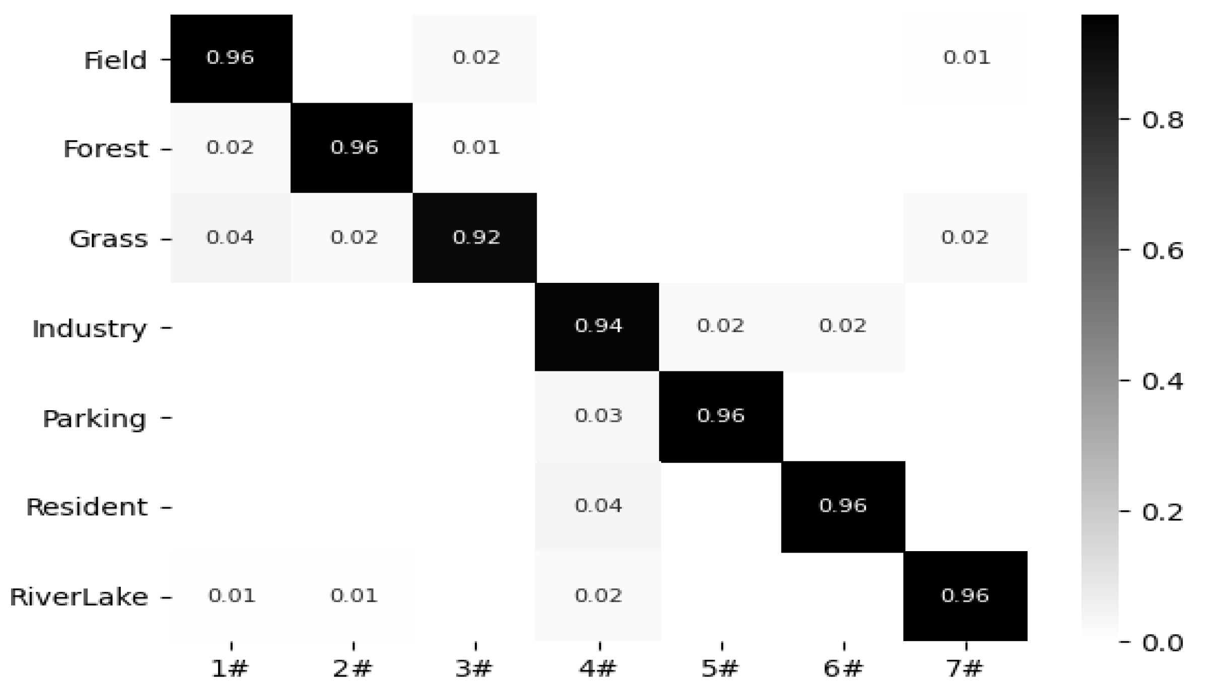
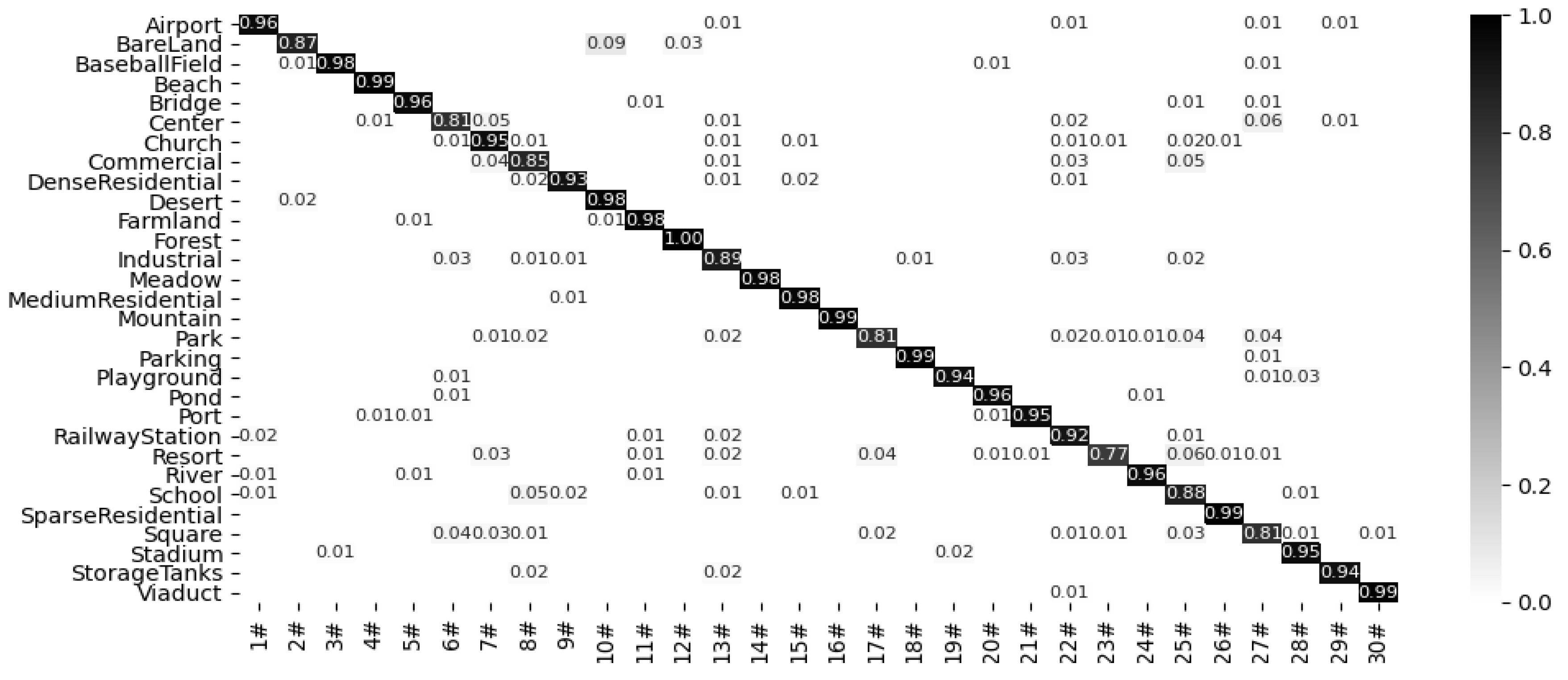
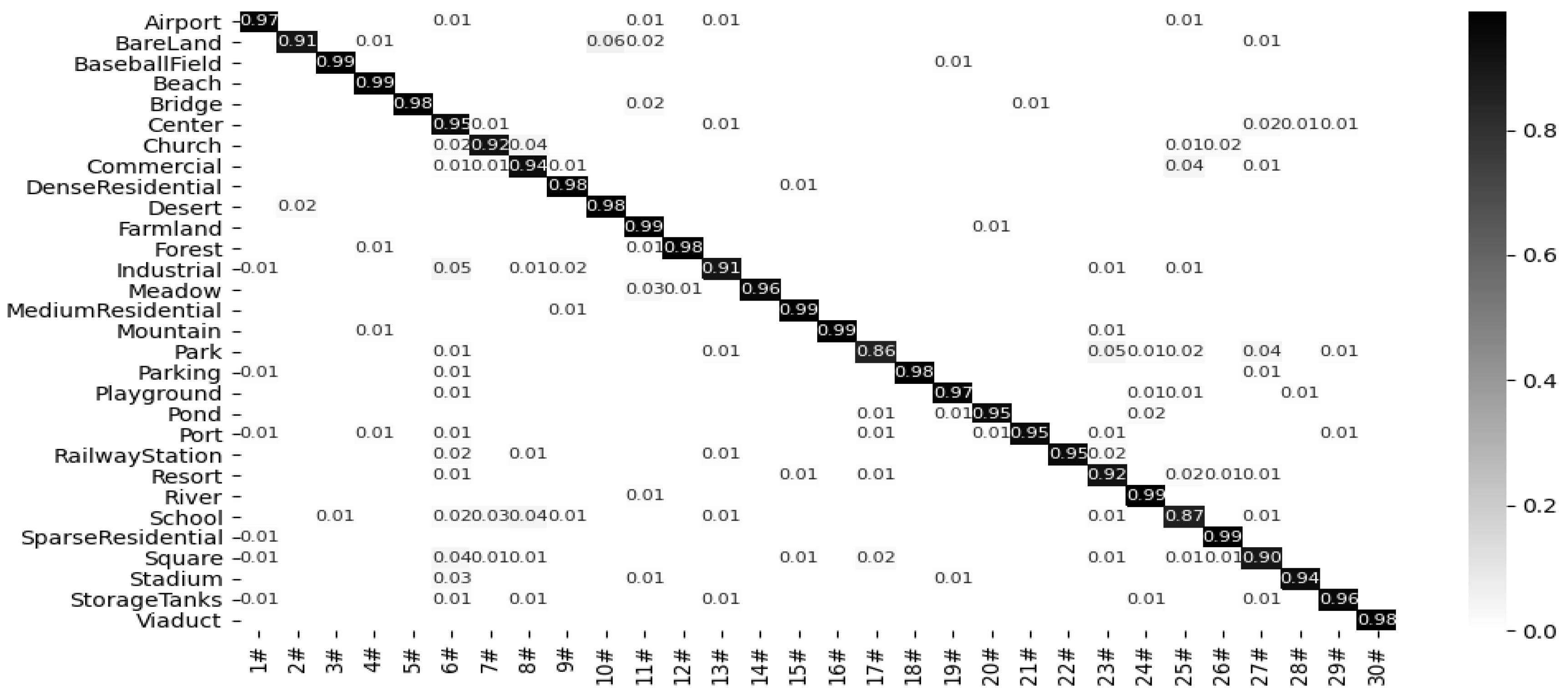
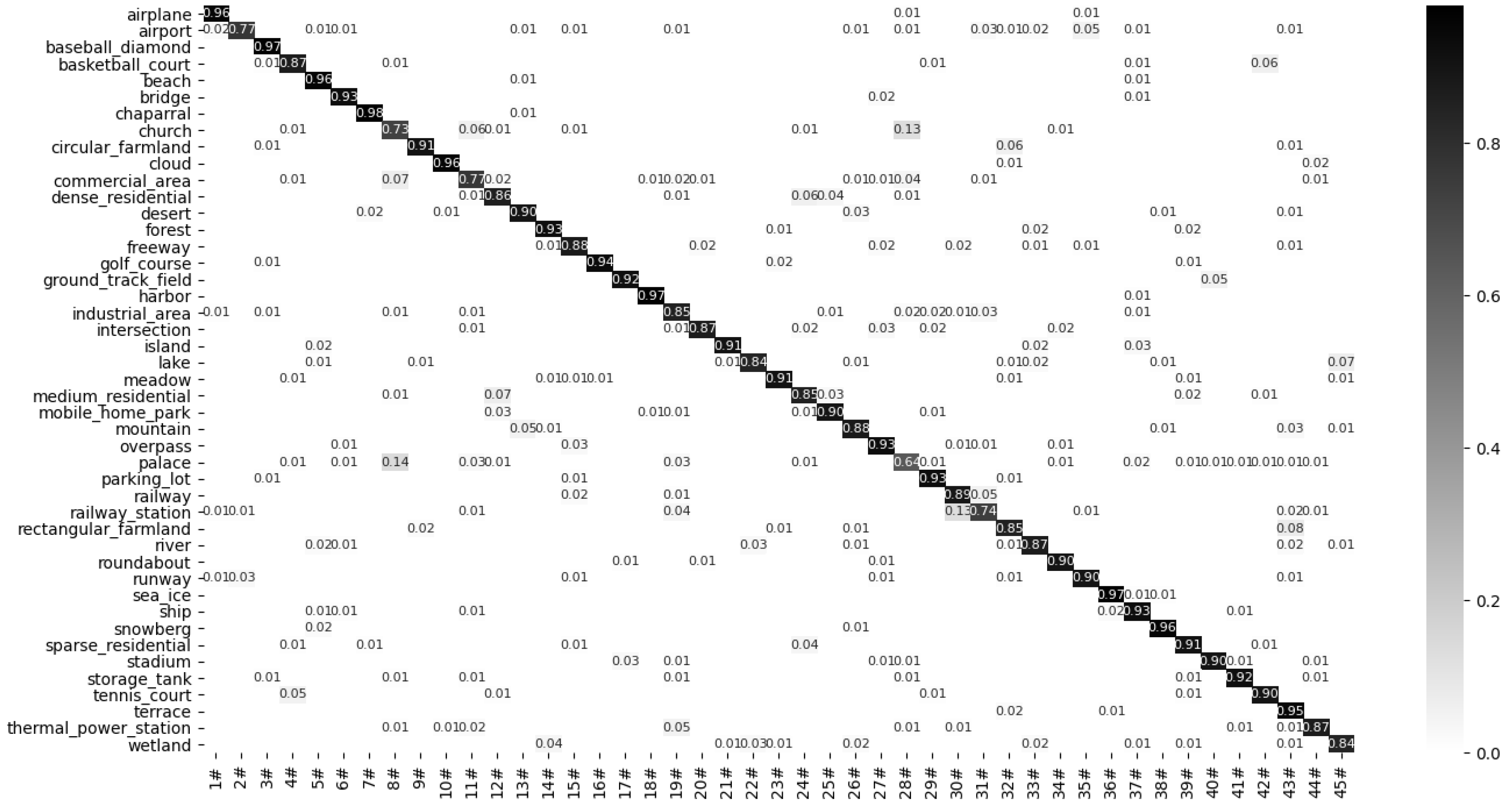
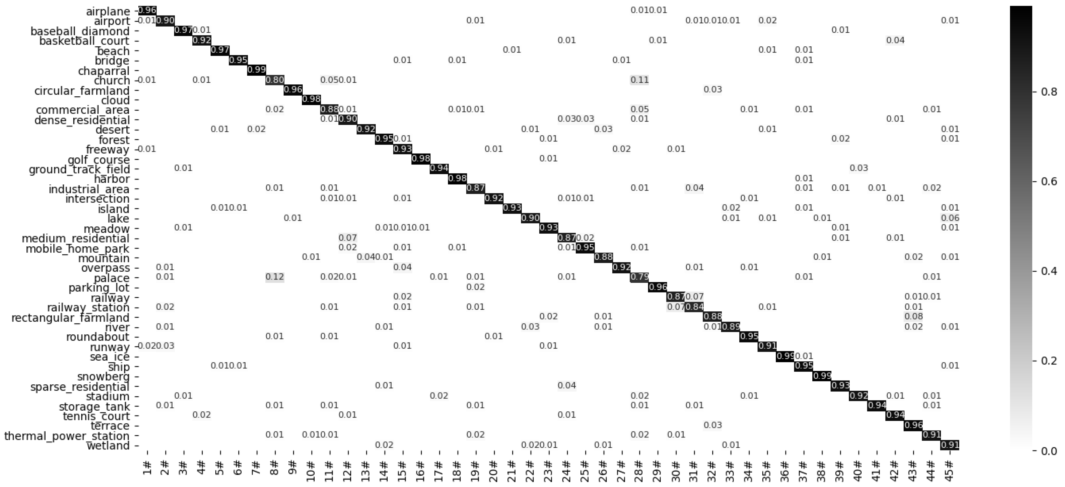
Figure 11, Figure 12, Figure 13, Figure 14 and Figure 15 show the confusion matrix of the proposed model under the RSSCN7 (50/50), AID (20/80), AID30 (50/50), NWPU45 (10/90), and NWPU45 (20/80) dataset partitions. The results show that the proposed model can obtain better classification results with multiple datasets. This indicates that after multi segment feature fusion, the proposed network model can better overcome the high similarity between remote sensing scene images.
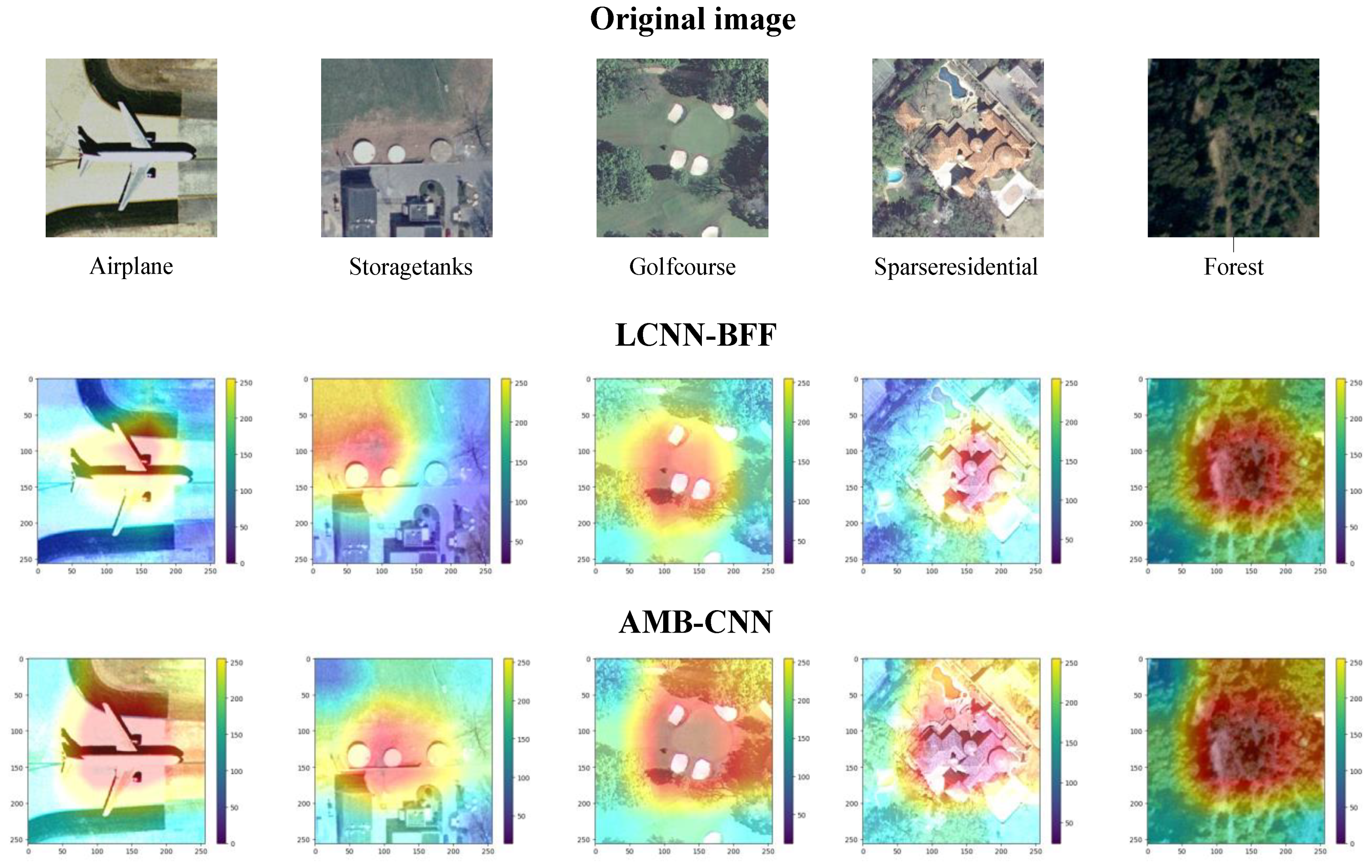
To comprehensively evaluate the proposed model from different perspectives, grad cam is used to visually analyze the different network models. This method can use the gradient of any target along with the last layer of the convolution network to generate a rough attention map, which can be used to display the important areas in the model prediction image. In the experiment, some images are selected randomly in the UCM21 dataset, and the latest LCNN-BFF method is compared with the proposed method. Some remote sensing scene images, including an aircraft, fuel tank, golf course, sparse residence, and forest, are randomly selected for comparison, as shown in Figure 16.
It can be seen in Figure 16 that for the scene of storage tanks, the focus area of the LCNN-BFF model is shifted, and the proposed AMB-CNN model can focus on the target object very well. For the airplane, golf course, sparse residence, and forest scenes, the focus areas of the LCNN-BFF are limited, and thus the regions surrounding the target are ignored. Therefore, the extracted targets are incomplete. However, the proposed model can still provide complete focus areas.
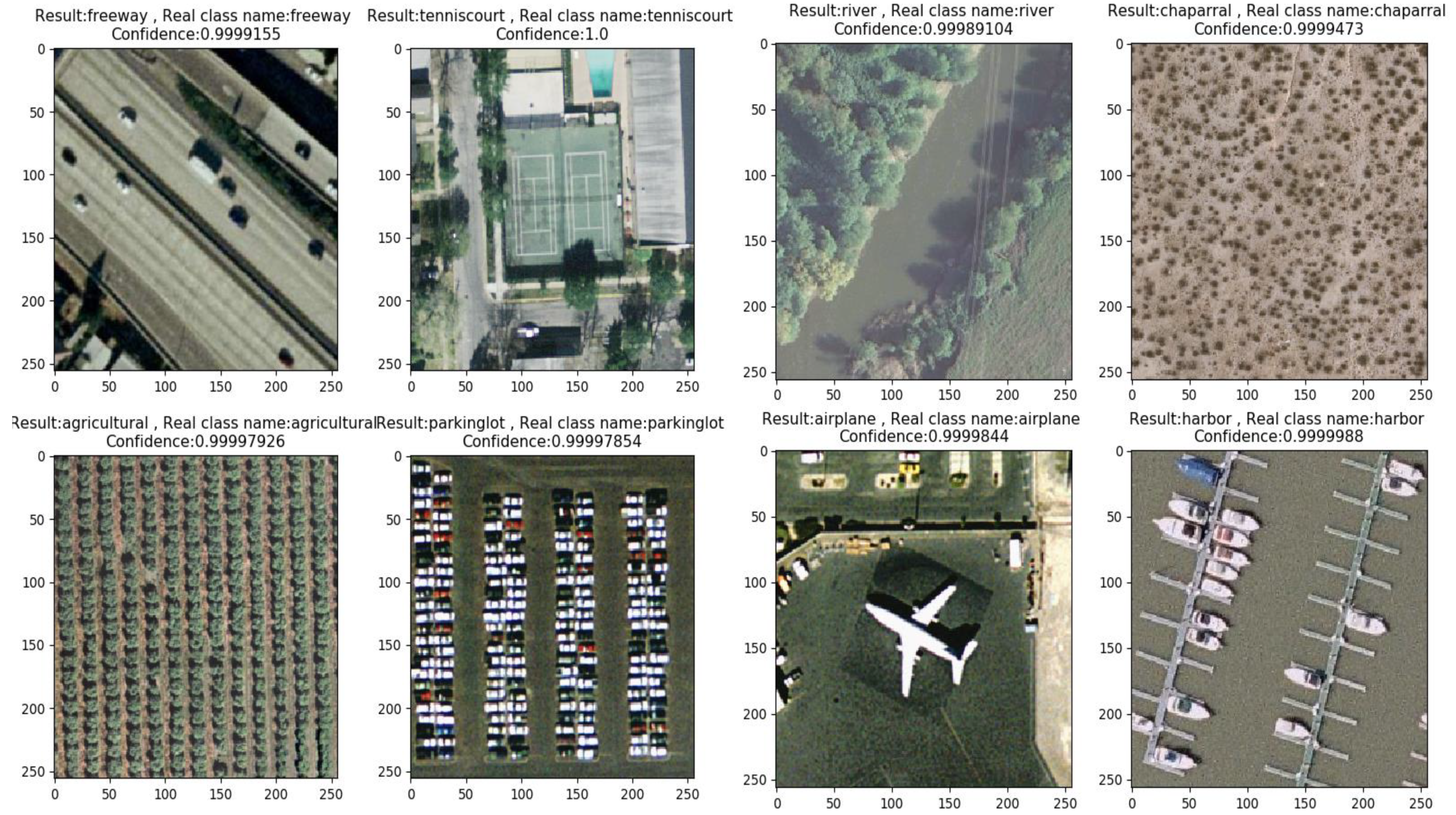
The trained network model is also tested with randomly selected images, as shown in Figure 17. We can see that the prediction results provided by the proposed model are consistent with the real scenarios, and the prediction confidences are all above 99%, with some individual scenarios reaching 100%. This proves that the proposed method can extract image features more effectively.
4. Discussion
4.1. Model Analysis
The proposed AMB-CNN method is evaluated on four datasets with different division proportions, and is proven to have a good classification performance. At the same time, the number of parameters for the proposed method is lower than that of the other advanced methods. These benefits come from the following two aspects. First, in the feature extraction stage, the model is divided into several modules, by which the shallow features and deep features are extracted. At the same time, considering the complexity of the model, a hybrid convolution method is adopted, and multiple small convolutions cascade instead of a large convolution. Secondly, in the aspect of feature fusion, with the multi segment attention mechanisms, the extracted features are input into the attention mechanism to extract important information again, and finally, the multi branch features are fused.
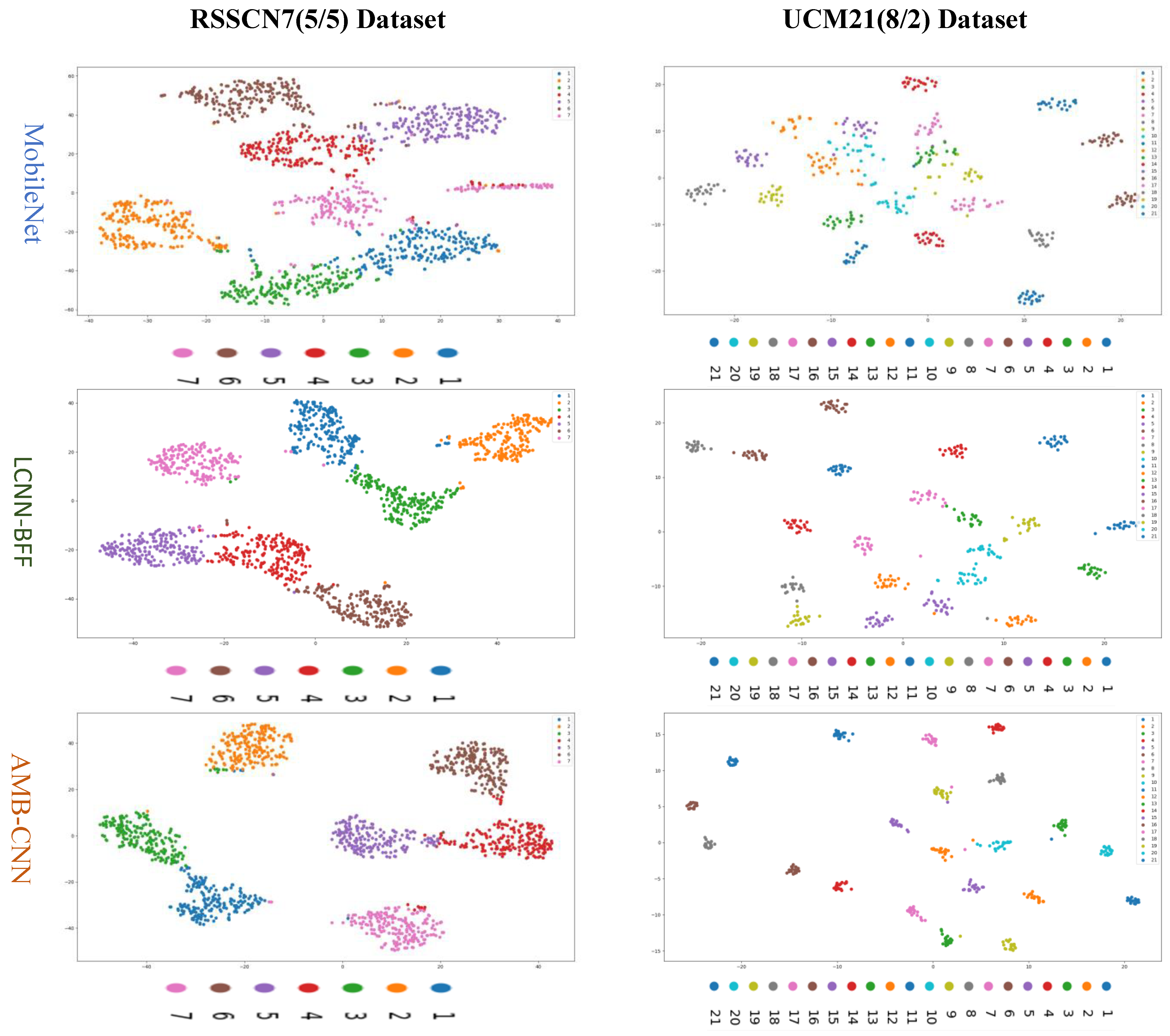
4.2. Visual Dimension Assessment
T-distributed stochastic neighbor embedding (T-SNE) visualization is adopted to further evaluate the performance of the AMB-CNN model. T-SNE data dimensionality reduction and visualization can better estimate the classification performance of the model by mapping high-dimensional data into two-dimensional space and using scatter distribution to visually display the classification effect. On the RSSCN7 (5/5) and UCM21 (8/2) datasets, the T-SNE visualization effects of MobileNet, LCNN-BFF, and the proposed AMB-CNN model are compared, as shown in Figure 18.
In Figure 18, we can see that compared with the other two methods, the classification results of the proposed method have a smaller intra class distance and larger inter class distance, which indicates that the proposed method can better extract image features and distinguish different categories, thereby providing an excellent performance for remote sensing image scene classification.
5. Conclusions
In this paper, a lightweight convolutional neural network based on attention-oriented multi-branch feature fusion (AMB-CNN) is proposed. This method has been proven to be effective with various datasets and under various conditions. A multi-branch convolution block is designed for feature extraction under a fully expanded receptive field. At the same time, the attention mechanism is utilized for feature weighting analysis of the spatial and channel information. Finally, all of the features are fused. In this way, not only are the key features extracted accurately, but the loss of information is also reduced. In addition, a network model with very low parameters is constructed through depthwise separable convolution and traditional convolution alternation. The experimental results show that compared with some state-of-the-art methods, the parameter of the proposed method is only 5.6 M, while still having a great advantage in classification accuracy. Especially on the UCM21 dataset, the OA of the proposed method is up to 99.52%, which exceeds that of most of the existing advanced methods. In addition, the proposed method also shows good performance on other datasets, such as the AID dataset with a training/test ratio of 2:8, where the OA of the proposed method reaches 93.27%. The next step is to extend this method to other remote sensing data, such as hyperspectral images, to improve the universality of the proposed model.
Author Contributions
Conceptualization, C.S.; data curation, C.S. and X.Z.; formal analysis, L.W.; methodology, C.S.; software, X.Z.; validation, C.S. and X.Z.; writing—original draft, X.Z.; writing—review and editing, C.S. and L.W. All authors have read and agreed to the published version of the manuscript.
Funding
This research was funded in part by the National Natural Science Foundation of China (41701479 and 62071084), in part by the Project plan of Science Foundation of Heilongjiang Province of China (under grant QC2018045), and in part by the Fundamental Research Funds in Heilongjiang Provincial Universities of China (under grant 135509136).
Acknowledgments
We would like to thank the handling editor and the anonymous reviewers for their careful reading and helpful remarks.
Conflicts of Interest
The authors declare no conflict of interest.
References
- Zheng, X.; Yuan, Y.; Lu, X. A Deep Scene Representation for Aerial Scene Classification. IEEE Trans. Geosci. Remote Sens. 2019, 57, 4799–4809. [Google Scholar] [CrossRef]
- Yuan, Y.; Fang, J.; Lu, X.; Feng, Y. Remote sensing image scene classification using rearranged local features. IEEE Trans. Geosci. Remote Sens. 2019, 57, 1779–1792. [Google Scholar] [CrossRef]
- Guo, Y.; Li, Y.; Zhu, L.; Wang, Q.; Lv, H.; Huang, C.; Li, Y. An Inversion-Based Fusion Method for Inland Water Remote Monitoring. IEEE J. Sel. Top. Appl. Earth Obs. Remote Sens. 2016, 9, 5599–5611. [Google Scholar] [CrossRef]
- Zhang, Y.; Zheng, X.; Yuan, Y.; Lu, X. Attribute-Cooperated Convolutional Neural Network for Remote Sensing Image Classification. IEEE Trans. Geosci. Remote Sens. 2020, 58, 8358–8371. [Google Scholar] [CrossRef]
- Li, E.; Xia, J.; Du, P.; Lin, C.; Samat, A. Integrating multilayer features of convolutional neural networks for remote sensing scene classification. IEEE Trans. Geosci. Remote Sens. 2017, 55, 5653–5665. [Google Scholar] [CrossRef]
- Li, Y.; Zhang, Y.; Huang, X.; Ma, J. Learning Source-Invariant Deep Hashing Convolutional Neural Networks for Cross-Source Remote Sensing Image Retrieval. IEEE Trans. Geosci. Remote Sens. 2018, 56, 6521–6536. [Google Scholar] [CrossRef]
- Lowe, D.G. Distinctive Image Features from Scale-Invariant Keypoints. Int. J. Comput. Vis. 2004, 60, 91–110. [Google Scholar] [CrossRef]
- Aude, O. Chapter 41—Gist of the Scene. In Neurobiology of Attention; Laurent, I., Geraint, R., John, K.T., Eds.; Academic Press: Cambridge, MA, USA, 2005; pp. 251–256. [Google Scholar]
- Dalal, N.; Triggs, B. Histograms of oriented gradients for human detection. In Proceedings of the IEEE Conference on Computer Vision and Pattern Recognition, San Diego, CA, USA, 20–25 June 2005; pp. 886–893. [Google Scholar]
- Gamage, P.T.; Azad, M.K.; Taebi, A.; Sandler, R.H.; Mansy, H.A. Clustering Seismocardiographic Events using Unsupervised Machine Learning. In Proceedings of the 2018 IEEE Signal Processing in Medicine and Biology Symposium (SPMB), Philadelphia, PA, USA, 1 December 2018; pp. 1–5. [Google Scholar]
- Risojevic, V.; Babic, Z. Unsupervised Quaternion Feature Learning for Remote Sensing Image Classification. IEEE J. Sel. Top. Appl. Earth Obs. Remote Sens. 2016, 9, 1521–1531. [Google Scholar] [CrossRef]
- Du, B.; Xiong, W.; Wu, J.; Zhang, L.; Zhang, L.; Tao, D. Stacked Convolutional Denoising Auto-Encoders for Feature Representation. IEEE Trans. Cybern. 2017, 47, 1017–1027. [Google Scholar] [CrossRef] [PubMed]
- Lecun, Y.; Bottou, L. Gradient-based learning applied to document recognition. Proc. IEEE 1998, 86, 2278–2324. [Google Scholar] [CrossRef] [Green Version]
- Krizhevsky, A.; Sutskever, I.; Hinton, G.E. Imagenet classification with deep convolutional neural networks. Commun. ACM 2012, 60, 1097–1105. [Google Scholar] [CrossRef]
- Simonyan, K.; Zisserman, A. Very deep convolutional networks for large-scale image recognition. arXiv 2014, arXiv:1409.1556. [Google Scholar]
- He, K.; Zhang, X.; Ren, S.; Sun, J. Deep residual learning for image recognition. In Proceedings of Proceedings of the IEEE conference on computer vision and pattern recognition, Las Vegas, NV, USA, 27–30 June 2016; pp. 770–778. [Google Scholar]
- Liu, Y.; Liu, Y.; Ding, L. Scene classification based on two-stage deep feature fusion. IEEE Geosci. Remote Sens. Lett. 2018, 15, 183–186. [Google Scholar] [CrossRef]
- Chaib, S.; Liu, H.; Gu, Y.; Yao, H. Deep Feature Fusion for VHR Remote Sensing Scene Classification. IEEE Trans. Geosci. Remote Sens. 2017, 55, 4775–4784. [Google Scholar] [CrossRef]
- Cheng, G.; Yang, C.; Yao, X.; Guo, L.; Han, J. When deep learning meets metric learning: Remote sensing image scene classification via learning discriminative CNNs. IEEE Trans. Geosci. Remote Sens. 2018, 56, 2811–2821. [Google Scholar] [CrossRef]
- Zhao, F.; Mu, X.; Yang, Z.; Yi, Z. A novel two-stage scene classification model based on feature variable significance in high-resolution remote sensing. Geocarto Int. 2019, 35, 1–12. [Google Scholar] [CrossRef]
- Iandola, F.N.; Han, S.; Moskewicz, M.W.; Ashraf, K.; Dally, W.J.; Keutzer, K. SqueezeNet: AlexNet-level accuracy with 50x fewer parameters and <0.5 MB model size. In Proceedings of the 5th International Conference on Learning Representations, ICLR 2017, Toulon, France, 24–26 April 2017; pp. 1–13. [Google Scholar]
- Howard, A.G.; Zhu, M.; Chen, B.; Kalenichenko, D.; Wang, W.; Weyand, T. MobileNets: Efficient convolutional neural networks for mobile vision applications. arXiv Prepr. 2017, arXiv:1704.04861. [Google Scholar]
- Zhang, W.; Tang, P.; Zhao, L. Remote sensing image scene classification using CNN-CapsNet. Remote Sens. 2019, 11, 494. [Google Scholar] [CrossRef] [Green Version]
- Zhao, Y.; Zhao, L.; Xiong, B.; Kuang, G. Attention Receptive Pyramid Network for Ship Detection in SAR Images. IEEE J. Sel. Topics Appl. Earth Observ. Remote Sens. 2020, 13, 2738–2756. [Google Scholar] [CrossRef]
- Cao, Y.; Ma, S.; Pan, H. FDTA: Fully Convolutional Scene Text Detection with Text Attention. IEEE Access 2020, 8, 155441–155449. [Google Scholar] [CrossRef]
- Lu, X.; Wang, B.; Zheng, X. Sound Active Attention Framework for Remote Sensing Image Captioning. IEEE Trans. Geosci. Remote Sens. 2019, 58, 1985–2000. [Google Scholar] [CrossRef]
- He, X.; Haffari, G.; Norouzi, M. Sequence to Sequence Mixture Model for Diverse Machine Translation. In Proceedings of the 22nd Conference on Computational Natural Language Learning, Brussels, Belgium, 31 October–1 November 2018; pp. 583–592. [Google Scholar]
- Lin, Z.; Feng, M.; dos Santos, C.N.; Yu, M.; Xiang, B.; Zhou, B.; Bengio, Y. A structured self-attentive sentence embedding. In Proceedings of the 5th International Conference on Learning Representations, ICLR 2017, Toulon, France, 24–26 April 2017; pp. 1–15. [Google Scholar]
- Wang, Q.; Liu, S.; Chanussot, J.; Li, X. Scene Classification With Recurrent Attention of VHR Remote Sensing Images. IEEE Trans. Geosci. Remote Sens. 2019, 57, 1155–1167. [Google Scholar] [CrossRef]
- Tong, W.; Chen, W.; Han, W.; Li, X.; Wang, L. Channel-Attention-Based DenseNet Network for Remote Sensing Image Scene Classification. IEEE J. Sel. Top. Appl. Earth Obs. Remote Sens. 2020, 13, 4121–4132. [Google Scholar] [CrossRef]
- Yu, D.; Guo, H.; Xu, Q.; Lu, J.; Zhao, C.; Lin, Y. Hierarchical Attention and Bilinear Fusion for Remote Sensing Image Scene Classification. IEEE J. Sel. Top. Appl. Earth Obs. Remote Sens. 2020, 13, 6372–6383. [Google Scholar] [CrossRef]
- Alhichri, H.; Alswayed, A.S.; Bazi, Y.; Ammour, N.; Alajlan, N.A. Classification of Remote Sensing Images Using EfficientNet-B3 CNN Model With Attention. IEEE Access 2021, 9, 14078–14094. [Google Scholar] [CrossRef]
- Yan, P.; He, F.; Yang, Y.; Hu, F. Semi-supervised representation learning for remote sensing image classification based on generative adversarial networks. IEEE Access 2020, 8, 54135–54144. [Google Scholar] [CrossRef]
- Wang, C.; Lin, W.; Tang, P. Multiple resolution block feature for remote-sensing scene classification. Int. J. Remote Sens. 2019, 40, 6884–6904. [Google Scholar] [CrossRef]
- Liu, X.; Zhou, Y.; Zhao, J.; Yao, R.; Liu, B.; Zheng, Y. Siamese convolutional neural networks for remote sensing scene classification. IEEE Geosci. Remote Sens. Lett. 2019, 16, 1200–1204. [Google Scholar] [CrossRef]
- Zhou, Y.; Liu, X.; Zhao, J.; Ma, D.; Yao, R.; Liu, B.; Zheng, Y. Remote sensing scene classification based on rotation-invariant feature learning and joint decision making. EURASIP J. Image Video Process. 2019, 2019, 3. [Google Scholar] [CrossRef] [Green Version]
- Lu, X.; Ji, W.; Li, X.; Zheng, X. Bidirectional adaptive feature fusion for remote sensing scene classification. Neurocomputing 2019, 328, 135–146. [Google Scholar] [CrossRef]
- Liu, Y.; Zhong, Y.; Qin, Q. Scene Classification Based on Multiscale Convolutional Neural Network. IEEE Trans. Geosci. Remote Sens. 2018, 56, 7109–7121. [Google Scholar] [CrossRef] [Green Version]
- Cao, R.; Fang, L.; Lu, T.; He, N. Self-Attention-Based Deep Feature Fusion for Remote Sensing Scene Classification. IEEE Geosci. Remote Sens. Lett. 2021, 18, 43–47. [Google Scholar] [CrossRef]
- Liu, B.D.; Meng, J.; Xie, W.Y.; Shao, S.; Li, Y.; Wang, Y. Weighted spatial pyramid matching collaborative representation for remote-sensing-image scene classification. Remote Sens. 2019, 11, 518. [Google Scholar] [CrossRef] [Green Version]
- He, N.; Fang, L.; Li, S.; Plaza, J.; Plaza, A. Skip-connected covariance network for remote sensing scene classification. IEEE Trans. Neural Netw. Learn. Syst. 2020, 31, 1461–1474. [Google Scholar] [CrossRef] [Green Version]
- He, N.; Fang, L.; Li, S.; Plaza, A.; Plaza, J. Remote sensing scene classification using multilayer stacked covariance pooling. IEEE Trans. Geosci. Remote Sens. 2018, 56, 6899–6910. [Google Scholar] [CrossRef]
- Sun, H.; Li, S.; Zheng, X.; Lu, X. Remote sensing scene classification by gated bidirectional network. IEEE Trans. Geosci. Remote Sens. 2020, 58, 82–96. [Google Scholar] [CrossRef]
- Lu, X.; Sun, H.; Zheng, X. A Feature Aggregation Convolutional Neural Network for Remote Sensing Scene Classification. IEEE Trans. Geosci. Remote Sens. 2019, 57, 7894–7906. [Google Scholar] [CrossRef]
- Lietal, B. Aggregated deep fisher feature for VHR remote sensing scene classification. IEEE J. Sel. Topics Appl. Earth Observ. Remote Sens. 2019, 12, 3508–3523. [Google Scholar]
- Boualleg, Y.; Farah, M.; Farah, I.R. Remote Sensing Scene Classification Using Convolutional Features and Deep Forest Classifier. IEEE Geosci. Remote Sens. Lett. 2019, 16, 1944–1948. [Google Scholar] [CrossRef]
- Xie, J.; He, N.; Fang, L.; Plaza, A. Scale-free convolutional neural network for remote sensing scene classification. IEEE Trans. Geosci. Remote Sens. 2019, 57, 6916–6928. [Google Scholar] [CrossRef]
- Zhang, D.; Li, N.; Ye, Q. Positional Context Aggregation Network for Remote Sensing Scene Classification. IEEE Geosci. Remote Sens. Lett. 2019, 17, 943–947. [Google Scholar] [CrossRef]
- Shi, C.; Wang, T.; Wang, L. Branch Feature Fusion Convolution Network for Remote Sensing Scene Classification. IEEE J. Sel. Top. Appl. Earth Obs. Remote Sens. 2020, 13, 5194–5210. [Google Scholar] [CrossRef]
- Li, J.; Lin, D.; Wang, Y.; Xu, G.; Zhang, Y.; Ding, C.; Zhou, Y. Deep Discriminative Representation Learning with Attention Map for Scene Classification. Remote Sens. 2020, 12, 1366. [Google Scholar] [CrossRef]
- Xia, G.-S.; Hu, J.; Hu, F.; Shi, B.; Bai, X.; Zhong, Y.; Zhang, L.; Lu, X. AID: A Benchmark Data Set for Performance Evaluation of Aerial Scene Classification. IEEE Trans. Geosci. Remote Sens. 2017, 55, 3965–3981. [Google Scholar] [CrossRef] [Green Version]
Figure 1.
The proposed attention-based multi branch feature fusion convolutional neural network (AMB-CNN) network model.
Figure 1.
The proposed attention-based multi branch feature fusion convolutional neural network (AMB-CNN) network model.

Figure 2.
Two module groups and feature fusion.

Figure 3.
Some samples from the UC Merced Land-Use Dataset (UCM21) dataset.

Figure 4.
Some samples from the AID30 dataset.

Figure 5.
Some samples from the RSSCN7 dataset.

Figure 6.
Some samples from the NWPU45 dataset.

Figure 7.
Comparison of the confusion matrix of the proposed method and MobileNet on the UCM21 dataset.
Figure 7.
Comparison of the confusion matrix of the proposed method and MobileNet on the UCM21 dataset.

Figure 8.
Average precision (AP) comparison results of the three methods for each category of the RSSCN7 (5/5) dataset.
Figure 8.
Average precision (AP) comparison results of the three methods for each category of the RSSCN7 (5/5) dataset.

Figure 9.
AP comparison results of the three methods for each category of the AID30 (2/8) dataset.

Figure 10.
AP comparison results of the three methods for each category of the NWPU45 (1/9) dataset.
Figure 10.
AP comparison results of the three methods for each category of the NWPU45 (1/9) dataset.

Figure 11.
Confusion matrix of the proposed method on the RSSCN7 dataset.

Figure 12.
Confusion matrix of the proposed method on the AID30 dataset (20/80).

Figure 13.
Confusion matrix of the proposed method on the AID30 dataset (50/50).

Figure 14.
Confusion matrix of the proposed method on the NWPU45 dataset (10/90).

Figure 15.
Confusion matrix of the proposed method on the NWPU45 dataset (20/80).

Figure 16.
A thermal diagram using the UCM21 dataset.

Figure 17.
Classification results with randomly selected images.

Figure 18.
T-distributed stochastic neighbor embedding (T-SNE) visualization analysis of the three methods.
Figure 18.
T-distributed stochastic neighbor embedding (T-SNE) visualization analysis of the three methods.


Table 1.
Performance comparison between MobileNet and the proposed method.
| DATA SET | MobileNet | AMB-CNN | ||||||
|---|---|---|---|---|---|---|---|---|
| OA(%) | KAPPA(%) | AP(%) | F1 | OA(%) | KAPPA(%) | AP(%) | F1 | |
| 80/20 UC | 97.62 | 97.50 | 97.71 | 97.61 | 99.52 | 99.50 | 99.55 | 99.52 |
| 20/80 AID | 87.21 | 86.76 | 87.43 | 87.18 | 93.27 | 93.04 | 93.05 | 92.99 |
| 50/50 AID | 92.12 | 91.84 | 92.24 | 92.11 | 95.44 | 95.38 | 95.50 | 95.42 |
| 10/90 NWPU | 82.66 | 82.27 | 82.74 | 82.60 | 88.99 | 88.74 | 89.04 | 88.95 |
| 20/80 NWPU | 87.85 | 87.57 | 87.89 | 87.81 | 92.42 | 92.25 | 92.50 | 92.43 |
| 50/50 RSSCN | 91.50 | 90.08 | 91.51 | 91.47 | 95.14 | 94.33 | 95.18 | 95.15 |
Table 2.
Performance comparison of the proposed model with some state-of-the-art methods on the UCM21 dataset.
Table 2.
Performance comparison of the proposed model with some state-of-the-art methods on the UCM21 dataset.
| The Network Model | OA(%) | Number of Parameters |
|---|---|---|
| Semi-supervised representation learning method [33] | 94.05 ± 1.2 | 210 M |
| Multiple resolution BlockFeature method [34] | 94.19 ± 1.5 | - |
| Siamese CNN [35] | 94.29 | - |
| Siamese ResNet50 with R.D method [36] | 94.76 | - |
| Bidirectional adaptive feature fusion method [37] | 95.48 | 130 M |
| Multiscale CNN [38] | 96.66 ± 0.90 | 60 M |
| VGG_VD16 with SAFF method [39] | 97.02 ± 0.78 | 15 M |
| Variable-weighted multi-fusion method [20] | 97.79 | - |
| ResNet+WSPM-CRC method [40] | 97.95 | 23 M |
| Skip-Connected CNN [41] | 98.04 ± 0.23 | 6 M |
| VGG16 with MSCP [42] | 98.36 ± 0.58 | - |
| Gated bidirectiona+global feature method [43] | 98.57 ± 0.48 | 138 M |
| Feature aggregation CNN [44] | 98.81 ± 0.24 | 130 M |
| Aggregated deep fisher feature method [45] | 98.81 ± 0.51 | 23 M |
| Discriminative CNN [19] | 98.93 ± 0.10 | 130 M |
| VGG16-DF method [46] | 98.97 | 130 M |
| Scale-free CNN [47] | 99.05 ± 0.27 | 130 M |
| Inceptionv3+CapsNet method [23] | 99.05 ± 0.24 | 22 M |
| Positional context aggregation method [48] | 99.21 ± 0.18 | 28 M |
| LCNN-BFF method [49] | 99.29 ± 0.24 | 6.2 M |
| DDRL-AM method [50] | 99.05 ± 0.08 | - |
| HABFNet [31] | 99.29 ± 0.35 | 6.2 M |
| EfficientNetB3-Attn-2 [32] | 99.21 ± 0.22 | - |
| The proposed AMB-CNN | 99.52 ± 0.11 | 5.6 M |
Table 3.
Performance comparison of the proposed model with some state-of-the-art methods on the RSSCN7 dataset.
Table 3.
Performance comparison of the proposed model with some state-of-the-art methods on the RSSCN7 dataset.
| The Network Model | OA(%) | Number of Parameters |
|---|---|---|
| VGG16+SVM method [51] | 87.18 | 130 M |
| Variable-weighted multi-fusion method [20] | 89.1 | - |
| TSDFF method [17] | 92.37 ± 0.72 | - |
| ResNet+SPM-CRC method [40] | 93.86 | 23 M |
| ResNet+WSPM-CRC method [40] | 93.9 | 23 M |
| LCNN-BFF method [49] | 94.64 ± 0.21 | 6.2 M |
| Aggregated deep Fisher feature method [45] | 95.21 ± 0.50 | 23 M |
| The proposed AMB-CNN | 95.14 ± 0.24 | 5.6 M |
Table 4.
Performance comparison of the proposed model with some state-of-the-art methods on the AID30 dataset.
Table 4.
Performance comparison of the proposed model with some state-of-the-art methods on the AID30 dataset.
| The Network Model | OA(20/80)(%) | OA(50/50)(%) | Number of Parameters |
|---|---|---|---|
| Bidirectional adaptive feature fusion method [37] | - | 93.56 | 130 M |
| VGG16+CapsNet [23] | 91.63 ± 0.19 | 94.74 ± 0.17 | 130 M |
| Feature aggregation CNN [44] | - | 95.45 ± 0.11 | 130 M |
| Discriminative +VGG16 [19] | 90.82 ± 0.16 | 96.89 ± 0.10 | 130 M |
| VGG16 with MSCP [42] | 91.52 ± 0.21 | 94.42 ± 0.17 | - |
| Fine-tuning method [51] | 86.59 ± 0.29 | 89.64 ± 0.36 | 130 M |
| Gated bidirectiona method [43] | 90.16 ± 0.24 | 93.72 ± 0.34 | 18 M |
| Gated bidirectiona+global feature method [43] | 92.20 ± 0.23 | 95.48 ± 0.12 | 138 M |
| VGG_VD16 with SAFF method [39] | 90.25 ± 0.29 | 93.83 ± 0.28 | 15 M |
| TSDFF method [17] | - | 91.8 | - |
| Discriminative+AlexNet [19] | 85.62 ± 0.10 | 94.47 ± 0.12 | 60 M |
| AlexNet with MSCP [42] | 88.99 ± 0.38 | 92.36 ± 0.21 | - |
| Skip-connected CNN [41] | 91.10 ± 0.15 | 93.30 ± 0.13 | 6 M |
| LCNN-BFF method [49] | 91.66 ± 0.48 | 94.64 ± 0.16 | 6.2 M |
| DDRL-AM method [50] | 92.36 ± 0.10 | 96.25 ± 0.05 | - |
| The proposed AMB-CNN | 93.27 ± 0.22 | 95.54 ± 0.13 | 5.6 M |
Table 5.
Performance comparison of the proposed model with some state-of-the-art methods on the NWPU45 dataset.
Table 5.
Performance comparison of the proposed model with some state-of-the-art methods on the NWPU45 dataset.
| The Network Model | OA(10/90)(%) | OA(20/80)(%) | Number of Parameters |
|---|---|---|---|
| VGG16+CapsNet [23] | 85.05 ± 0.13 | 89.18 ± 0.14 | 130 M |
| Discriminative with AlexNet [19] | 85.56 ± 0.20 | 87.24 ± 0.12 | 130 M |
| Discriminative with VGG16 [19] | 89.22 ± 0.50 | 91.89 ± 0.22 | 130 M |
| R.D method [36] | - | 91.03 | - |
| AlexNet with MSCP [42] | 81.70 ± 0.23 | 85.58 ± 0.16 | - |
| VGG16 with MSCP [42] | 85.33 ± 0.17 | 88.93 ± 0.14 | - |
| VGG_VD16 with the SAFF method [39] | 84.38 ± 0.19 | 87.86 ± 0.14 | 15 M |
| Fine-tuning method [51] | 87.15 ± 0.45 | 90.36 ± 0.18 | 130 M |
| Skip-connected CNN [41] | 84.33 ± 0.19 | 87.30 ± 0.23 | 6 M |
| LCNN-BFF method [49] | 86.53 ± 0.15 | 91.73 ± 0.17 | 6.2 M |
| The proposed AMB-CNN | 88.99 ± 0.14 | 92.42 ± 0.14 | 5.6 M |
Publisher’s Note: MDPI stays neutral with regard to jurisdictional claims in published maps and institutional affiliations. |
© 2021 by the authors. Licensee MDPI, Basel, Switzerland. This article is an open access article distributed under the terms and conditions of the Creative Commons Attribution (CC BY) license (https://creativecommons.org/licenses/by/4.0/).
Share and Cite
MDPI and ACS Style
Shi, C.; Zhao, X.; Wang, L. A Multi-Branch Feature Fusion Strategy Based on an Attention Mechanism for Remote Sensing Image Scene Classification. Remote Sens. 2021, 13, 1950. https://0-doi-org.brum.beds.ac.uk/10.3390/rs13101950
AMA Style
Shi C, Zhao X, Wang L. A Multi-Branch Feature Fusion Strategy Based on an Attention Mechanism for Remote Sensing Image Scene Classification. Remote Sensing. 2021; 13(10):1950. https://0-doi-org.brum.beds.ac.uk/10.3390/rs13101950
Chicago/Turabian StyleShi, Cuiping, Xin Zhao, and Liguo Wang. 2021. "A Multi-Branch Feature Fusion Strategy Based on an Attention Mechanism for Remote Sensing Image Scene Classification" Remote Sensing 13, no. 10: 1950. https://0-doi-org.brum.beds.ac.uk/10.3390/rs13101950
Note that from the first issue of 2016, this journal uses article numbers instead of page numbers. See further details here.