
GIS-Based Landslide Susceptibility Mapping of the Circum-Baikal Railway in Russia Using UAV Data


1
Siberian School of Geosciences, Irkutsk National Research Technical University, Lermontova St. 89, 664074 Irkutsk, Russia
2
Vinogradov Institute of Geochemistry SB RAS, Favorsky St. 1A, 664033 Irkutsk, Russia
3
SibGIS Tech LLC, Berezovy 112, 664523 Markova, Russia
*
Author to whom correspondence should be addressed.
Remote Sens. 2021, 13(18), 3629; https://0-doi-org.brum.beds.ac.uk/10.3390/rs13183629
Submission received: 16 July 2021
/
Revised: 31 August 2021
/
Accepted: 8 September 2021
/
Published: 11 September 2021
(This article belongs to the Special Issue Application of UAVs in Geo-Engineering for Hazard Observation)
Abstract
:The investigation of hard-to-reach areas that are prone to landslides is challenging. The research of landslide hazards can be significantly advanced by using remote sensing data obtained from an unmanned aerial vehicle (UAV). Operational acquisition and high detail are the advantages of UAV data. The development of appropriate automated algorithms and software solutions is necessary for quick decision-making based on the received heterogeneous spatial data characterising various aspects of the environment. This article introduces the first phase of a long-term study about landslide detection and prediction that aims to develop an automatic algorithm for detecting potentially hazardous landslide areas, using data obtained by UAV surveys. As a part of the project, the selection of appropriate techniques was implemented and a landslide susceptibility (LS) map of the study site was developed. This paper presents the outcomes of the applied indirect heuristic approach of landslide susceptibility assessment using an analytical hierarchy process (AHP) in a GIS environment, based on UAV data. The results obtained have been tested on a real-world entity.
1. Introduction
There is about 86,000 kms of railway tracks in Russia [1]. A considerable part of the railways is located in severe climatic and geomorphological conditions, and some areas along the lines are prone to landslides [2]. Since rail infrastructure is an essential part of communication between the regions of the country, geo-hazards can cause significant damage and financial loss [1]. Therefore, improving landslide detecting methods and developing new approaches are required for taking preventive actions to avoid the unfavourable consequences of landslide occurrence [3,4]. Landslide susceptibility (LS) mapping is a step towards a landslide hazard risk assessment of railways.
Traditional methods of landslide detection are commonly based on field surveys, in situ measurements, and visual analysis produced by an expert. Pedestrian tracking of potential collapse sites located in areas with difficult terrain is hazardous and time-consuming and does not provide a complete picture of the condition of the slope. To a certain degree, the results obtained are highly influenced by the knowledge and qualification of an expert [5]. The adoption of remote sensing techniques for landslide detection has great advantages compared to field surveys [6]. At the regional level, to solve problems associated with mudflow hazards, Earth Remote Sensing (ERS) data from satellites (multispectral and radar) are often used, the advantage of which is accessibility to any territory, and the absence of the need for terrestrial field research. However, low-resolution satellite images are not able to reveal the condition of slopes close to the rails, as slope angles reach 80 degrees and the distance between the landslide and railway can be up to 2 m. Satellite imagery data provide images with a maximum resolution of 0.5 m, which is insufficient for highly detailed mapping [7]. Recently, UAV surveys have become an available method of obtaining highly detailed ERS data. When surveying at heights of the order of 100–150 m, images obtained from multispectral cameras commonly used on UAVs reach the first centimetres per pixel. In addition, another advantage of low-altitude UAV surveys is that high-resolution satellite data are quite expensive and cannot be guaranteed to be obtained on the required date, due both to weather conditions and to the frequency of a satellite pass [8]. Therefore, the adoption of UAV-based data for geological hazard assessment stems from cost- and time-efficiency, optical and temporal resolution, and scope to explore inaccessible areas. It is important to note that in our study, unlike many other cases, there is no problem of access to the survey site, since the survey areas are adjacent to the railway. In this regard, the key advantage of the satellite images—accessibility to hard-to-reach areas—is not so significant.
Different features affecting the probability of landslides can be derived from remote sensing data. Thus, UAV or satellite imagery allows the generation of a Digital Surface Model (DSM) and, if the vegetation on the site is not too dense, a Digital Terrain Model (DTM), which makes it possible to determine the steepness of slopes, terrain ruggedness, and other parameters that directly affect the risk of landslide occurrence. UAV images are used to create a precise DSM and DTM from a dense point cloud, generated using desktop photogrammetry software [4]. UAV-derived DTM allows the detection of micro-landforms not identifiable in DTM at coarser scales [9]. Additionally, due to the high detail of the UAV survey, we can filter out individual trees and obtain the DTM from the DSM. Data as regards the presence and type of vegetation, superficial fissuring, etc., are just as important as data describing the landform. Such ground surface information can be derived from multispectral or hyperspectral surveys, which are currently widely implemented in both satellite and UAV-based observations [10]. Some research uses UAV data for DTM creation only, and adopts low-resolution satellite data for spectral data extraction [11]. Using high-resolution multispectral cameras allows us to compute spectral indices with a great degree of accuracy, which is crucial in local large-scale mapping. However, Alimohammadlou et al. [5] define issues associated with using remote sensing in landslide data acquisition. In some cases, it is hardly possible to distinguish active or old landslide bodies from the surrounding landforms, especially if they are concealed by vegetation [9]. The main issue is the need to involve an expert whatever technique is adopted.
Thus, various ERS data make it possible to create reliable maps of the facts of the occurred landslides, and monitor their progress. However, an equally interesting and more urgent task for our “railway problem” is forecasting new landslides, which begins with identifying the most favourable areas, based on a complex of morphostructural and multispectral data. According to Ray et al. [12], many researchers have used spatial, low resolution remotely sensed data for landslide prediction at a global and regional scale. A large number of scientific works are known in which low-altitude UAV survey technologies have been successfully used in landslide research to solve problems such as fine-scale mapping, monitoring, and analysis of active landslides [13,14,15,16,17]. However, there is a lack of landslide susceptibility research based on highly detailed UAV data.
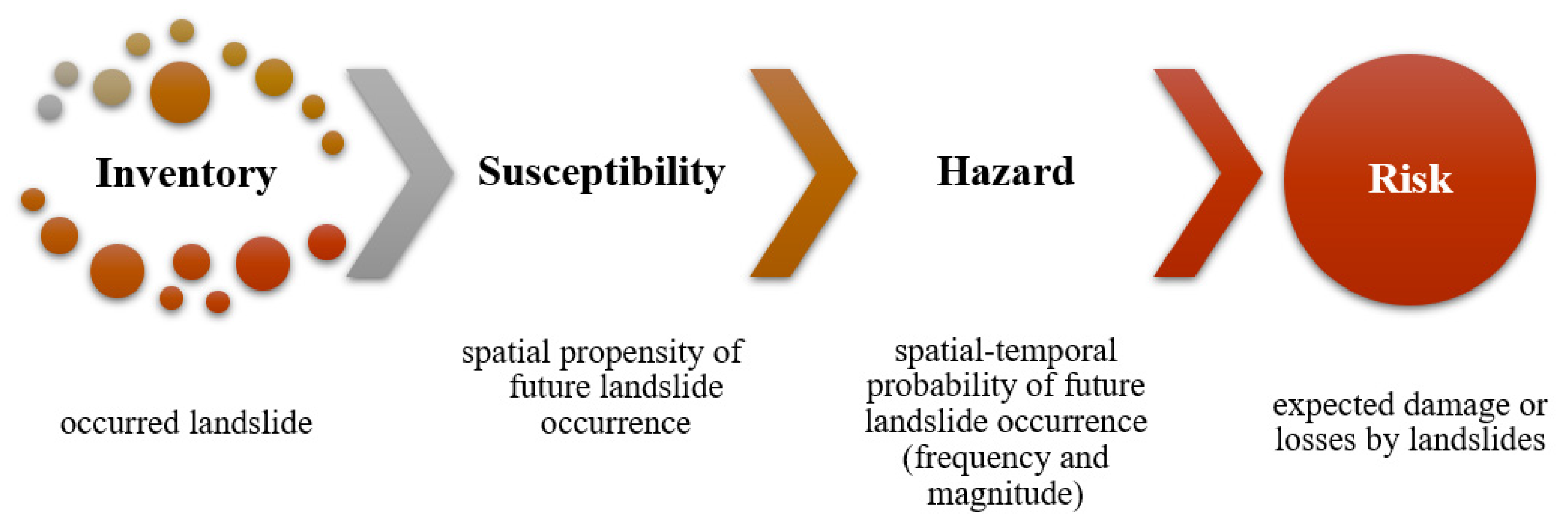
The spatial likelihood of landslide occurrence—susceptibility—is an initial delineation of zones prone to landslides due to a number of conditional and triggering factors [3,18]. The mapping of high-susceptibility zones aims to be aware of potentially hazardous slopes that need to be investigated in order to prescribe landslide prevention and mitigation measures [19]. It is worth underlining that the terms of landslide susceptibility and landslide hazard are often mistakenly considered synonymous [20]. Van Westen [21] describes “levels” of landslide mapping (Figure 1).
LS assessment considers the spatial allocation of landslide-prone areas, whereas hazard mapping introduces temporal characteristics and delivers frequency, volume, and transformations of landslides further. Barredo et al. [22] and Hervás and Bobrowsky [6] describe methods of landslide susceptibility assessment and their pros and cons (Figure 2). The authors compare direct and indirect approaches and consider that combining methods has shown good results. A deterministic approach requires accurate measurements of geotechnical parameters for model development and slope stability analysis; however, such data are not always possible to collect. Statistical approach effectiveness depends upon a massive amount of data on historical records of previous landslides and their characteristics. Thus, in the absence of detailed field data, the most commonly used is the heuristic indirect approach. Sabokbar et al. [23] show a consimilar landslide susceptibility mapping (LSM) classification from a different perspective, where the distinguishing of qualitative, quantitative, and hybrid methods is based on whether they are data-driven or knowledge-driven.
This article provides the technology for identifying the most landslide-hazardous areas for the infrastructure of the Trans-Siberian Railway, using multispectral UAV imagery and data processing techniques. In the example of one of the sections of the Circum-Baikal Railway, the results of an indirect heuristic approach applied to the assessment of landslide probability using an analytical hierarchy process (AHP) in a GIS environment are represented. Thus, we hope to solve the problem of reliably mapping the most dangerous areas, so that later, after the accumulation of statistics on the frequency of landslides in different areas, it will be possible to give a quantitative forecast of the probability of a landslide, based on its recommendations on the frequency of monitoring surveys.
2. Materials and Methods
2.1. Study Area
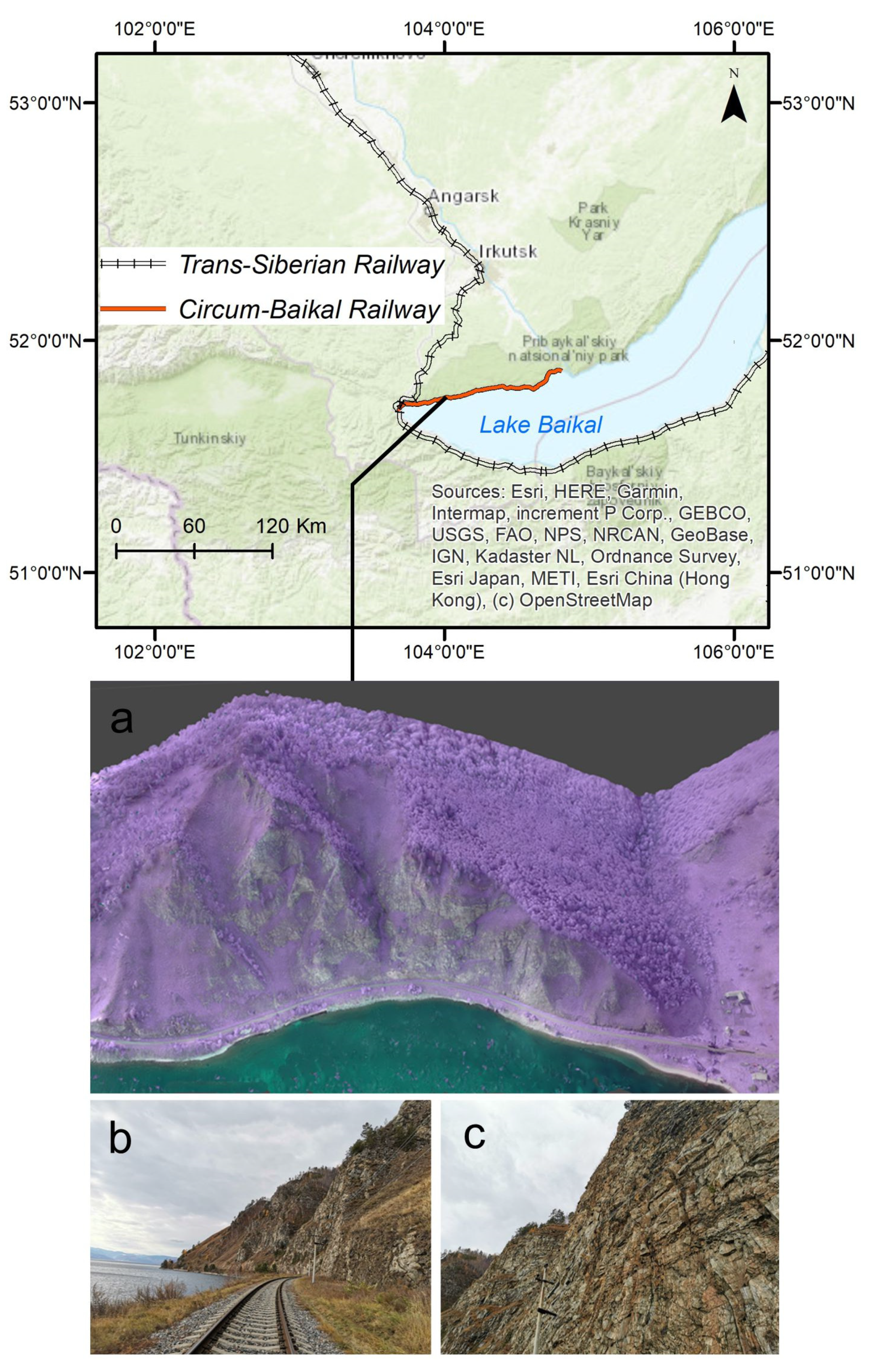
The Circum-Baikal Railway is located in the Irkutsk Region, Russia (Figure 3). The Circum-Baikal Railway is a historic railway, the construction of which began at the end of the 19th century. Nowadays, it is operated predominantly for a touristic purpose, but similar conditions are typical for other sections of the Trans-Siberian Railway and the Baikal-Amur Mainline. The Circum-Baikal Railway was chosen as a convenient test site because trains pass through it relatively rarely. The railway tracks are placed on a ledge surrounded by the coastline of Lake Baikal on the one side, and sheer cliffs reaching an angle of inclination of up to 80 degrees on the other side. Due to the use of explosives during construction in already difficult terrain, landslides often occur in this area. Landslides can damage railway tracks and electrical communications, as well as coastal protection structures, which leads to accelerated destruction of the ledge [24]. Damage repair requires significant financial and labour expenses. Therefore, the task of creating methods for performing aerial photogrammetry for monitoring landslide processes and places of a possible collapse of steep slopes of the Circum-Baikal Railway is very urgent. The study site is located near the railway stop, 27 km from the Slyudyanka settlement, the starting point for the Circum-Baikal Railway.
2.2. UAV Data Acquisition and Pre-Processing
An unmanned system SibGIS UAS created and operated for the geophysical survey was used for data acquisition (Table 1, Figure 4). The SibGIS UAS is a hexacopter weighing about 8 kg (including cameras and gimbal), and the diagonal of its frame is about one metre. Since the payload is lightweight, we intend to use lighter UAVs in the future.
Two cameras, the characteristics of which are shown in Table 2, were installed on a three-axis gyro-stabilised gimbal. As will be shown below, the use of a heavier three-axis gimbal is highly desirable, since when shooting with tilt cameras, the UAV will always fly one side forward.
The cameras are equipped with built-in satellite antennas that allow the recording of the exact time of the image acquisition in the metadata. However, in order to be able to comprehensively process all six spectral channels, to create multispectral composites and calculate multispectral pixel-to-pixel indices, it is necessary to take pictures absolutely synchronously so that the boundaries of the images from both cameras coincide. To do this, our system uses the standard Pixhawk flight controller technology to simultaneously trigger the cameras (https://www.mapir.camera/blogs/guide/trigger-survey-camera-from-pixhawk-flight-controller (accessed on 10 September 2021)).
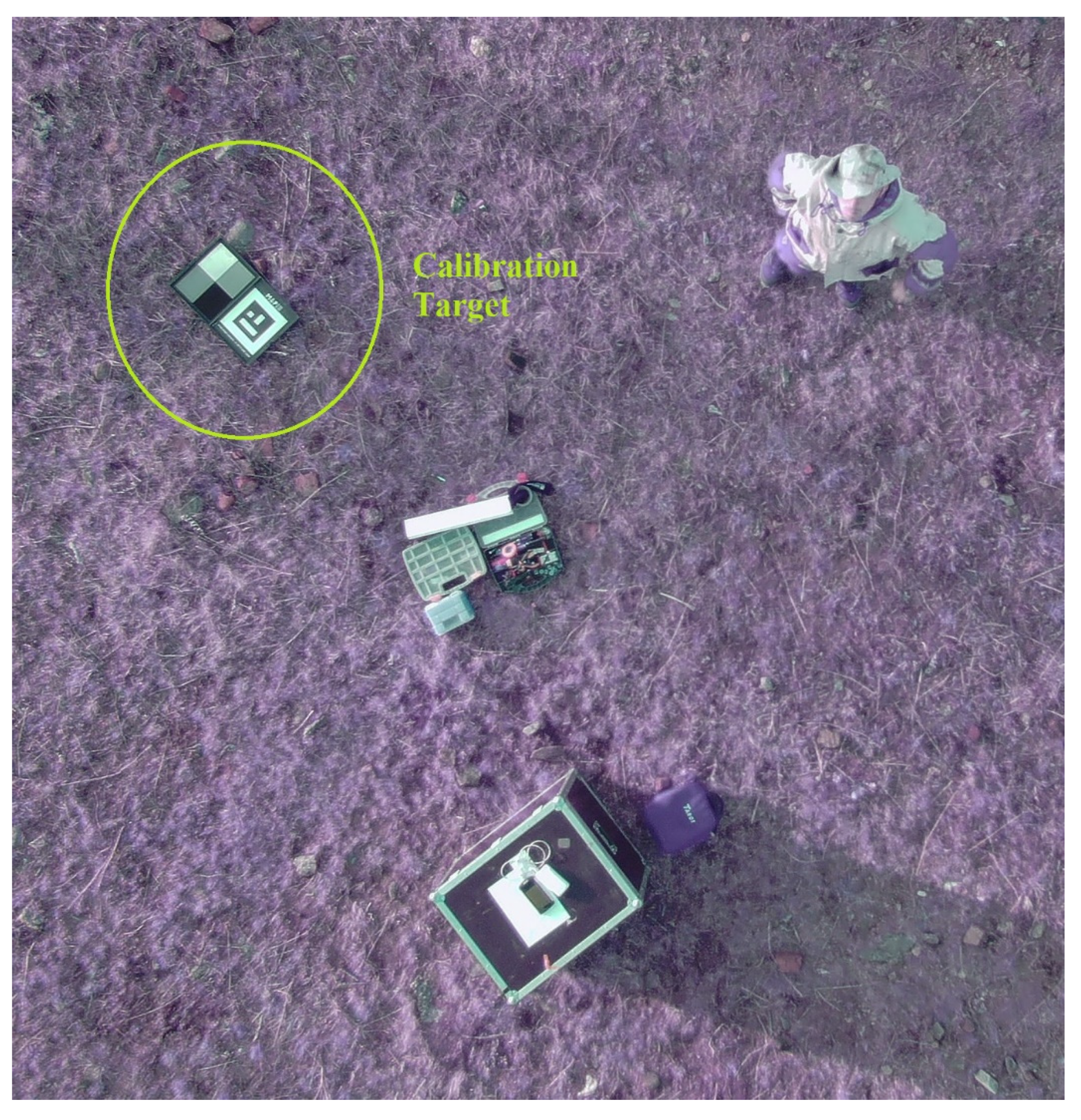
Photographing is carried out in the RAW format, so we captured a percentage of reflectance of sunlight in each pixel of the images. Because the illumination changes during surveying, it is necessary to calibrate the obtained images using a reference reflectance value. Many serial multispectral cameras, for example, the Parrot Sequoia, have a built-in sunshine sensor that constantly records lighting conditions in the same spectral channels as on the camera and allows us to automatically receive already calibrated images. Our cameras were not equipped with such sensors. We performed the calibration by capturing a photo of the special tool—MAPIR Calibration Ground Target (Figure 5)—which contains 4 targets that have been measured at incremental wavelengths by a calibrated lab spectrometer. The pixel values of the captured target image were then compared with the known reflectance values of the targets. Using the MAPIR Camera Control (MCC) application, we then transformed the pixel values and thus calibrated the survey images.
As a result, we obtained spectral images that allowed us to calculate common indices, such as NDVI, according to standard formulas, and classify and interpret them according to generally accepted legends.
Once the images were calibrated, we stitched them together into a single ortho-mosaic and DTM, using Structure from Motion (SFM) technology. In order to obtain a high-quality result, it is necessary to have centimetre-accurate coordinates of the images. In our case, high-precision image georeferencing was provided by RTK (Real Time Kinematic) technology. Before the start of surveying, the “base” of the satellite navigation geodetic system was installed, which recorded raw GNSS data. The “rover” was the GNSS antenna of the UAV. The RTK system allowed the continuous transmitting of GNSS corrections to the UAV using a radiotelemetry system, which ensured the recording of the coordinates of centimetre-accuracy in the memory of the flight controller in real time. Since the survey sites have an area of no more than the first tens of square kilometres, there was constant radiocommunication between the UAV and the ground station. Otherwise, we would be forced to use coordinate post-processing kinematic (PPK) technology, which would take more time. After the survey was completed, the precise coordinates from the UAV GNSS antenna were entered into the metadata of the images, instead of the low-precision coordinates from the antennas built into the cameras based on the unity of satellite time. For this, the GeoSetter software was used.
The site described in the article is characterised by extremely steep terrain, and elevation differences of hundreds of metres per kilometre of the area. Concerning this, an accurate terrain-following is required [25]. The terrain-following planning mode is comprised of keeping a constant altitude above ground level during the flight [26]. We applied the SibGIS Flight Planner technique developed by Parshin et al. [27], which allows the performance of flight missions to collect an array of points—“longitude-latitude-altitude”—while all points are at a constant height above a predetermined DTM. In this case, Intermap NEXTmap data with a spatial resolution of 10 m were used as a given DTM. The survey was carried out at an altitude of 125 m above the ground. At this height, the resolution of obtained images is 5.7 cm per pixel for 12-megapixel cameras. The survey was carried out along a network of parallel routes, and the longitudinal overlap between frames is 70–80% and the cross-sectional overlap is 60–70% to enable three-dimensional reconstruction of the terrain, adopting image matching algorithms.
Initially, we attempted to use nadir photography—the traditional photogrammetry technique—but in this case, it was impossible to reconstruct the sections of the steepest slopes (Figure 6).
The advantage of UAV surveys over satellite surveys in this case is the ability to perform surveys with different camera tilt angles, which is widely used, for example, when creating digital models of buildings. Taking into account the sizes of objects that are significantly larger than in architectural tasks, it was necessary to determine the minimum and sufficient set of camera tilt angles that would allow us to obtain high-quality digital terrain models without excessively increasing the field work time, the amount of data, and the time of photogrammetric calculations. It turned out that the best option is capturing from two camera tilt angles of 45 and 90 (nadir) degrees. It can be noticed in Figure 7 that the high-resolution imagery of the sub-vertical sections of the slopes makes it possible to significantly detail such parameters as terrain roughness, in comparison with the nadir imagery—both UAV and satellite. Regarding the need to use spectral bands other than the visible light spectrum, OCN filters (Figure 4a) have some advantages in distinguishing vegetation and soil due to wider band widths and the NIR value of 808 nm, instead of the more commonly used 850 nm, supplying more contrast [28]. As soil commonly has reflectance in the red spectrum, it leads to “soil noise pixel”; using orange light allows us to avoid the blurring effect and clearly discern boundaries of soil and vegetation. It is important to precisely highlight vegetation cover as its presence may reduce vertical accuracy and cause distortions of the DTM [29].
Using photogrammetry software OpenDroneMap, an SFM algorithm can be performed based on the obtained aerial photography data with high-precision coordinates in the metadata of images. SFM derives matching features on the set of images to generate X, Y, and Z positions of a dense point cloud. As a result of the photogrammetry process, a 3D model, multispectral (six channels) orthophoto, and DTM were obtained. Then, vegetation index and morphological indices were computed using the raster calculator tools in GIS. We did not use ground points to refine the referencing of the obtained results, since at this stage of the study it was not high absolute accuracy for comparing the models obtained at different times that was important to us, but only a high-resolution DEM with high relative accuracy, which allowed us to calculate the morphostructural characteristics of the relief with high detail.
2.3. LS Parameters
The significant stage of the LS analysis is the distinction of suitable conditioning and triggering factors that depend on geological, topographic, and environmental conditions and anthropogenic disturbances [3,6,30,31]. The choice of characteristics is very important for the spatial forecasting of landslides; the use of an excessive number of parameters can distort the accuracy of the assessment [32]. Psomiadis et al. [4] determined procedures for LS estimation—defining conditioning parameters affecting propensity to slope failure, and choosing an appropriate technique for the factors’ weights determination. GIS allows the application of parameter map overlay to receive a susceptibility map [18]. In the absence of expensive geotechnical survey data, the adoption of GIS-based combined landslide assessment techniques is comparable in complexity and an effective method at local scale [22]. However, the results are highly dependent on the correct selection of the parameters for considering unique landscape conditions. As was mentioned above, the main disadvantage of direct and indirect approaches is that they rely on the implementor’s competence to a great extent, and the subjectivity of landslide assessment approaches is almost unavoidable. However, an expert’s contribution can be reduced by applying an analytical hierarchy process for the designation of the extent of the parameters’ impact, i.e., weights of factors. There are many multi-criteria evaluation techniques that can be adopted for susceptibility assessment. The most common are AHP (analytical hierarchy process), logical regression model, frequency ratio model, fuzzy logic, etc. According to Nguyen and Liu [31], there are five most commonly applied factors of slope instability at global and regional scales: slope angle, lithology, land cover, drainage density, and aspect. Land cover and lithology are estimated based on multispectral images, while other parameters are derived from DTM. Since we are engaged in slope instability detection on a local scale, lithology is not considered due to its invariability within the study area. Other parameters may be addressed by highly detailed data received from the UAV.
We also did not take into account other regional parameters, since they do not change locally within the site. However, the parameter variation should be considered when examining larger areas. Landslide occurrence likelihood depends on climatic conditions due to impact on temperature, moisture, and wind [33]. Unique landscape features such as underlying permafrost soils should be considered as they could have a crucial influence on the other parameters. Hence, some of the criteria involved in landslide processes are to be established according to the area conditions, and there are two possible approaches: either delineate zones of similar conditions along the research area, or simplify the method by reducing the subset of data to an extent that could fit and work on any territory. “Tendency to simplify the factors that condition landslides” [34] is a good practice when automatising the process is required; however, the accuracy and the reliability of results are likely to decrease to some degree. Nevertheless, simplified universal algorithms considering the assumptions of any mathematical and computed-based algorithms, due to complexity or scarcity of data, are working practices.
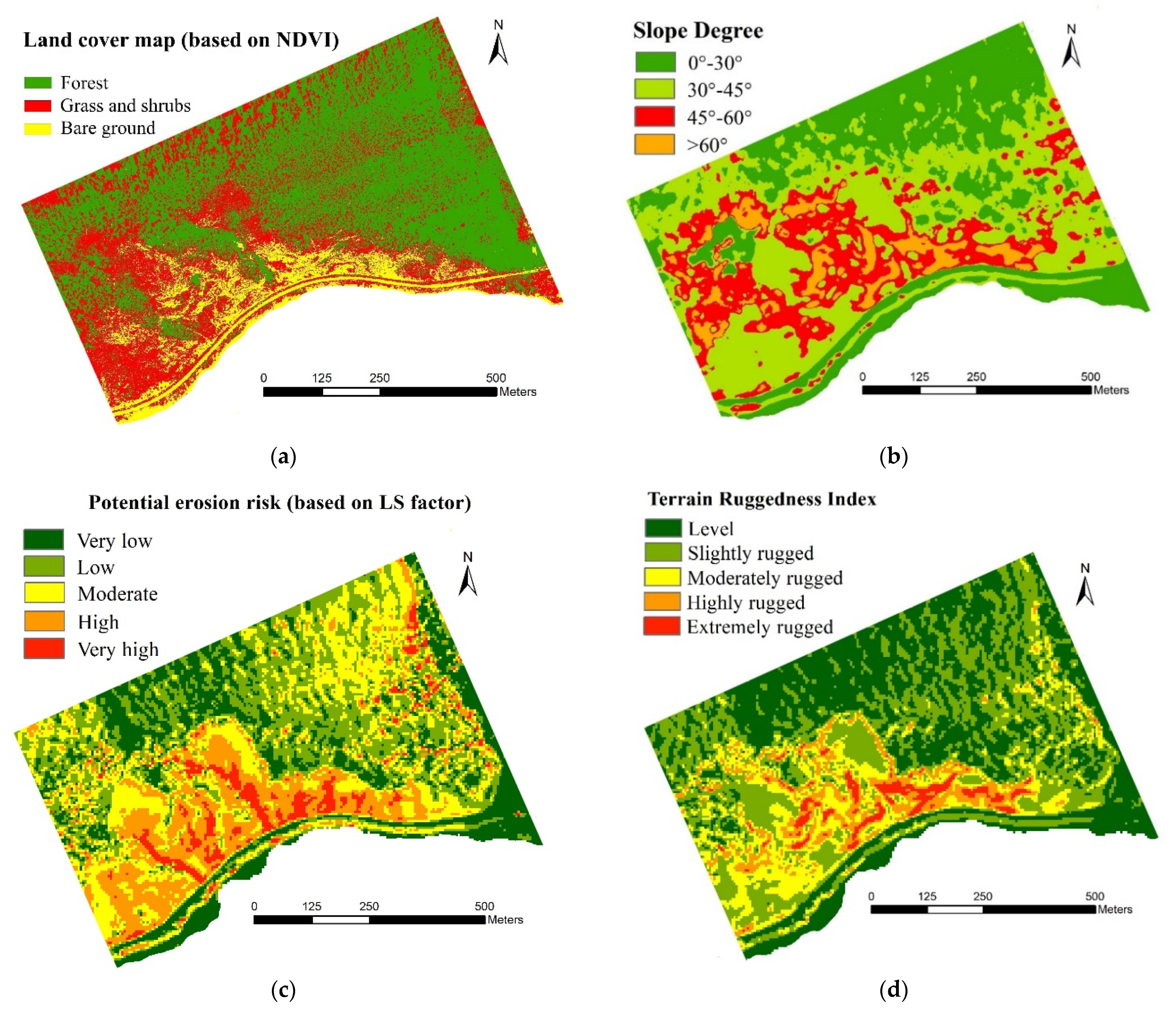
The accuracy of LS directly depends on the set of factors taken into account. According to Bhatt et al. [35], areas covered by dense forest are less prone to landslides. Song et al. [36] explain that tree roots contribute to the strengthening of slopes and reduce the wetness of soil. The Normalised Difference Vegetation Index (NDVI) is commonly applied to distinct land cover types [4]. It uses an infrared spectral band to indicate vegetation, soil, water bodies, and artificial landscape elements. As an OCN camera was used in our study, the red band in the NDVI calculation was replaced by an orange one. A modified NDVI was generated using calibrated images obtained using the OCN camera and multispectral sensor. Pixel-based supervised land cover classification was implemented [37], then values were reclassified to reduce the number of classes to three that are sufficient for the study of land cover types (Figure 8a): forested area, grass and shrubs area, and bare ground. Forested areas are set to be non-landslide. Grassland is considered to be a low impact factor, and bare ground is a high susceptibility area.
Landslide occurrence has a direct dependency on terrain steepness; thus, slope is a key factor in LS mapping [31,38]. Steepness was subdivided into four classes: slope less than 30 degrees, from 30 to 45 degrees, from 45 to 60 degrees, and slope angle greater than 60 degrees (Figure 8b). Though slope length has a lower impact on ground movement than slope steepness, longer slopes result in higher flow rates of landslide masses [39]. The risk of erosion increases with the steepness and length of the slope. Some researchers consider the greater the slope gradient, the higher the landslide susceptibility [31]. In fact, areas with a slope gradient greater than 60 degrees consist of stable rocks, thus slope between 45–60 degrees has a higher landslide susceptibility. An LS factor (length and steepness), a combined parameter defining potential soil erosion risk, is used in this research in addition to the slope angle parameter [40]. The LSF was classified as very low, low, moderate, high, and very high (Figure 8c).
Różycka et al. [41] analysed the relation between the distribution of parameters derived from a high-resolution DTM—Topographic Wetness Index (TWI) and Terrain Ruggedness Index (TRI)—and landslide allocations. The authors found that areas of high TWI values overlap with the landslide bodies; moreover, they indicate the most probable direction of the landslide. TWI is the natural logarithm of the ratio of the drainage area to the slope. The higher the index value, the greater the moisture content in the soil. TRI reflects the relative local vertical roughness of the terrain and can be measured as the average value of the height difference between each cell and the surrounding cells. High TRI values clearly indicate steep scarps, while areas of slightly rugged TRI values feature source areas of landslides (Figure 8d). The reclassified TWI map shows drainage directions that match with preferential landslide pathways (Figure 8e). TRI and TWI were calculated in SAGA GIS for LSM. TWI values were divided into 4 groups and the TRI ranged from level to extremely rugged areas.
Hence, the following factors are considered in our study: slope angle, TWI, LSF, TRI, and land cover (vegetation). An AHP model, through pairwise comparison, was used to determine the conditioning factors’ contribution to landslide susceptibility. The LS index is computed by the following formula:
is the weight of the factor and is the weight of the class within the factor. An AHP method [42] was applied for the definition of the contribution of each factor to LS.
Table 3 displays the matrix of pairwise comparison reflecting the priority of each factor over another in agreement with the scale introduced by Saaty [43]. Table 4 shows another level of the AHP matrix, embracing classes within the factors. The consistency ratio of each calculated parameter is less than 0,1; consequently, the determination of weights can be considered reliable.
3. Results
Corresponding layers are generated in a GIS environment. QGIS, SAGA GIS, and ArcGIS software can be applied to implement a weighted overlay for receiving the LS map. Figure 9 shows that LS was classified as low, moderate, high, and very high susceptability areas. In percentage terms, a high and a very high LS index is observed in about 13% of the study site.
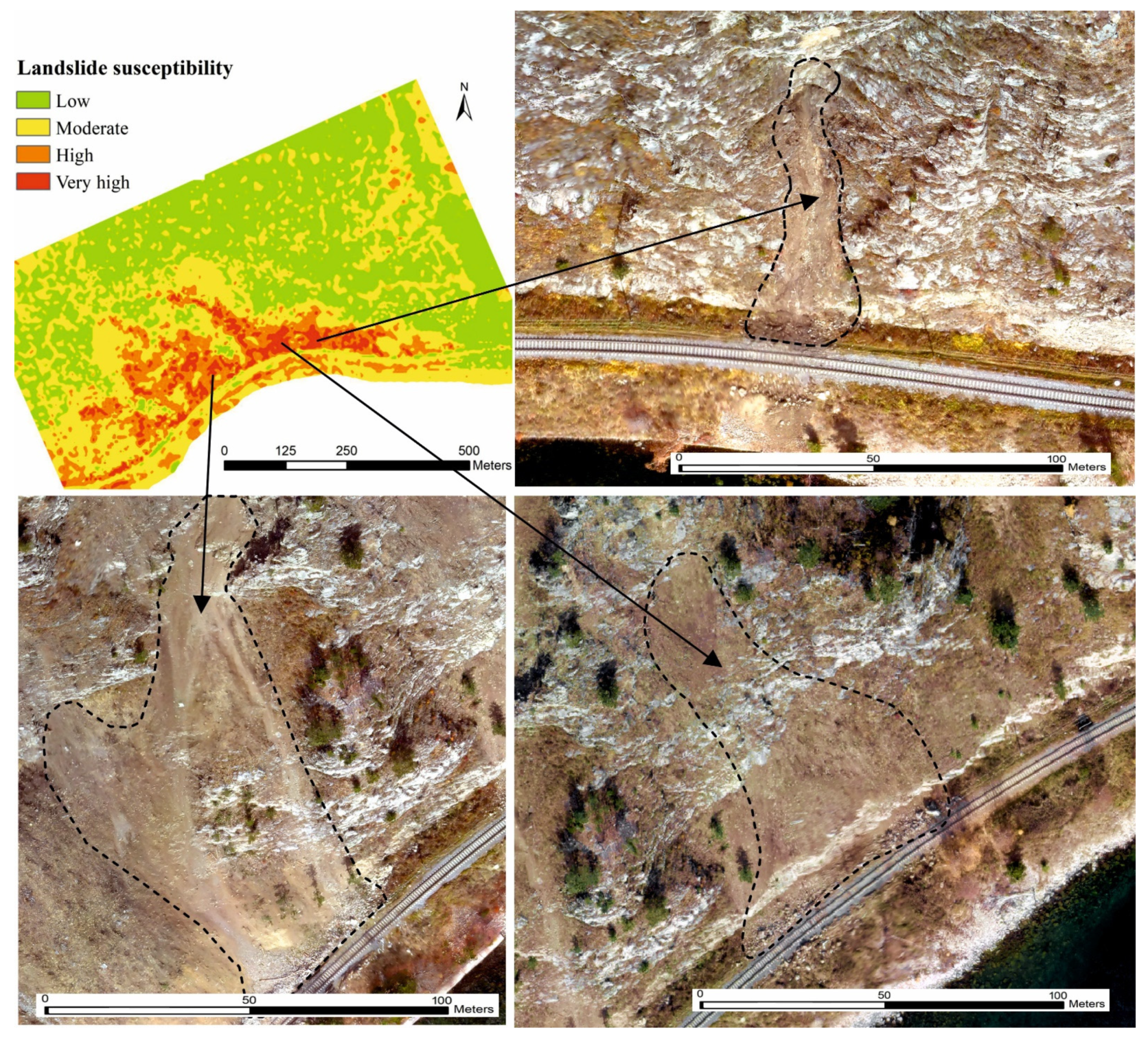
The areas with high and very high susceptibility are expected to warrant further closer investigation. The obtained result is verified by comparison with inventory survey data depicting existing landslides and the interpretation of aerial images (Figure 10). According to long-term observations in this area for the period from 1930 to 2019, 24 landslide events occurred in those areas that we have identified as especially dangerous. Russian Railways collect data with a step of 1 km of railway track, and only record landslides that have caused significant damage to the railway infrastructure; therefore, statistical data are not tied to certain small sections of slopes. Based on internal Russian Railways data, we cannot perform a quantitative classification of landslide susceptibility by comparing the degree of manifestation of the trait according to our forecast with the average annual probability of landslides, or other quantitative hazard parameters. In 2020, during our survey, we recorded three cases of landslides, which are shown in Figure 10, confirming the correctness of our forecasting results on a qualitative level. The results can be refined using classical methods of geomorphological research, sampling, on-site measurements, etc. Repeated surveys using UAV will allow the application of data for time-series image processing for comparing multitemporal data and revealing changes. Change detection can assess the accuracy of the forecast of the likelihood of landslide occurrence.
4. Conclusions
In this article, we performed a landslide susceptibility assessment of a section of the Circum-Baikal Railway. The study demonstrates reliable qualitative level detection of hazardous areas based on UAV imagery and derived geomorphometric and spectral indices. The key concept of adopting the approach used is the fast, cost-effective, and simple way of delineating high landslide susceptibility areas using datasets obtained remotely, which is crucial in hard-to-reach areas. The drawback of the applied LS mapping technology is using an excessive amount of external soft packages at different stages of the research. Therefore, our future studies will seek to design a system that consolidates computing and analysis stages from different programs to one environment. This would remove the need for the participation of experts at each stage of data processing. Further research is also planned to enhance the accuracy of the outcomes and the promptness of obtaining the results. The desired outcome is to collect a sufficient amount of data to produce hazard and risk assessment models enclosing temporal and volume probabilistic characteristics.
The main disadvantage of the study at its current stage, in our opinion, is that so far we have not been able to solve the problem of quantifying the probability of landslide descent, which is necessary to optimise the monitoring frequency of each site. For this, it is necessary to compare the conditional values of landslide susceptibility «low–moderate–high–very high» to the average frequency of landslides in the area of each class. This is due to the lack of a sufficient amount of reliable data on previous landslide events. Therefore, the next step of our research is to quantitatively evaluate landslide hazards on different sites with various frequencies of landslide occurrence, which will allow us “to calibrate” and validate the consistency of the applied method.
Author Contributions
Conceptualization and methodology, S.G. and A.P.; software, data acquisition, and pre-processing, V.E.; writing—original draft preparation, S.G.; writing—review and editing, A.P.; supervision, A.P. All authors have read and agreed to the published version of the manuscript.
Funding
The work was supported by the Ministry of Science and Higher Education of the Russian Federation, grant No. 075-15-2020-787.
Acknowledgments
The authors are grateful to Vladislav Kasperovich (JSCo “Russian Railways”) for the provided data on landslide statistics for 1930–2019.
Conflicts of Interest
The authors declare no conflict of interest.
References
- Gadelshina, L.A.; Vakhitova, T.M. The Place and Role of Transport Infrastructure in the Interregional Integration of the Russian Federation Regions. In Proceedings of the International Conference on Applied Economics ICOAE 2015, Kazan Russia, 2–4 July 2015; Volume 24, pp. 246–250. [Google Scholar] [CrossRef] [Green Version]
- Akkerman, G.; Akkerman, S.; Mironov, A. Design of the railway track infrastructure of the subpolar and northern regions. MATEC Web Conf. 2018, 216, 02017. [Google Scholar] [CrossRef]
- Pourghasemi, H.R.; Rossi, M. Landslide susceptibility modeling in a landslide prone area in Mazandarn Province, north of Iran: A comparison between GLM, GAM, MARS, and M-AHP methods. Theor. Appl. Climatol. 2017, 130, 609–633. [Google Scholar] [CrossRef]
- Psomiadis, E.; Papazachariou, A.; Soulis, K.X.; Alexiou, D.-S.; Charalampopoulos, I. Landslide Mapping and Susceptibility Assessment Using Geospatial Analysis and Earth Observation Data. Land 2020, 9, 133. [Google Scholar] [CrossRef]
- Alimohammadlou, Y.; Tanyu, B.F.; Abbaspour, A.; Delamater, P.L. Automated landslide detection model to delineate the extent of existing landslides. Nat. Hazards 2021, 107, 1639–1656. [Google Scholar] [CrossRef]
- Hervás, J.; Bobrowsky, P. Mapping: Inventories, Susceptibility, Hazard and Risk. In Landslides—Disaster Risk Reduction; Sassa, K., Canuti, P., Eds.; Springer: Berlin/Heidelberg, Germany, 2009; pp. 321–349. [Google Scholar] [CrossRef]
- Schultz, N. High Resolution Remote Sensing Using UAS Technology. Available online: https://hixon.yale.edu/sites/default/files/files/fellows/paper/schultz_hixon_final_121517.pdf (accessed on 10 April 2021).
- Eisenbeiß, H. UAV Photogrammetry; ETH Zurich: Zurich, Switzerland, 2009. [Google Scholar]
- Chudý, F.; Slámová, M.; Tomaštík, J.; Prokešová, R.; Mokroš, M. Identification of Micro-Scale Landforms of Landslides Using Precise Digital Elevation Models. Geosciences 2019, 9, 117. [Google Scholar] [CrossRef] [Green Version]
- Jackisch, R.; Lorenz, S.; Zimmermann, R.; Möckel, R.; Gloaguen, R. Drone-Borne Hyperspectral Monitoring of Acid Mine Drainage: An Example from the Sokolov Lignite District. Remote Sens. 2018, 10, 385. [Google Scholar] [CrossRef] [Green Version]
- Sun, X.; Chen, J.; Bao, Y.; Han, X.; Zhan, J.; Peng, W. Landslide Susceptibility Mapping Using Logistic Regression Analysis along the Jinsha River and Its Tributaries Close to Derong and Deqin County, Southwestern China. ISPRS Int. J. Geo-Inf. 2018, 7, 438. [Google Scholar] [CrossRef] [Green Version]
- Ram, L. Ray Remote Sensing Approaches and Related Techniques to Map and Study Landslides. In Landslides; Lazzari, M., Ed.; IntechOpen: Rijeka, Croatia, 2020; p. 2. [Google Scholar] [CrossRef]
- Rossi, G.; Tanteri, L.; Tofani, V.; Vannocci, P.; Moretti, S.; Casagli, N. Multitemporal UAV surveys for landslide mapping and characterization. Landslides 2018, 15, 1045–1052. [Google Scholar] [CrossRef] [Green Version]
- Niethammer, U.; Rothmund, S.; Joswig, M. UAV-based remote sensing of the slow-moving landslide Super-Sauze. In Proceedings of the International Conference on Landslide Processes: From Geomorpholgic Mapping to Dynamic Modelling, Strasbourg, France, 6–7 February 2009; pp. 69–74. [Google Scholar]
- Afif, H.A.; Saraswati, R.; Hernina, R. UAV Application for Landslide Mapping in Kuningan Regency, West Java. E3S Web Conf. 2019, 125, 03011. [Google Scholar] [CrossRef] [Green Version]
- Peppa, M.; Mills, J.; Moore, P.; Miller, P.; Chambers, J. Accuracy assessment of a UAV-based landslide monitoring system. ISPRS-Int. Arch. Photogramm. Remote Sens. Spat. Inf. Sci. 2016, 41, 895–902. [Google Scholar] [CrossRef] [Green Version]
- Lindner, G.; Schraml, K.; Mansberger, R.; Hübl, J. UAV monitoring and documentation of a large landslide. Appl. Geomat. 2016, 8, 1–11. [Google Scholar] [CrossRef]
- Dai, F.C.; Lee, C.F.; Ngai, Y.Y. Landslide risk assessment and management: An overview. Eng. Geol. 2002, 64, 65–87. [Google Scholar] [CrossRef]
- Pradhan, B. A comparative study on the predictive ability of the decision tree, support vector machine and neuro-fuzzy models in landslide susceptibility mapping using GIS. Comput. Geosci. 2013, 51, 350–365. [Google Scholar] [CrossRef]
- Fell, R.; Corominas, J.; Bonnard, C.; Cascini, L.; Leroi, E.; Savage, W.Z. Guidelines for landslide susceptibility, hazard and risk zoning for land-use planning. Eng. Geol. 2008, 102, 99–111. [Google Scholar] [CrossRef] [Green Version]
- Van Westen, C. National Scale Landslide Susceptibility Assessment for Saint Vincent. Master's Thesis, University of Twente, Enschede, The Netherlands, 2016. [Google Scholar]
- Barredo, J.; Benavides, A.; Hervás, J.; van Westen, C.J. Comparing heuristic landslide hazard assessment techniques using GIS in the Tirajana basin, Gran Canaria Island, Spain. Int. J. Appl. Earth Obs. Geoinf. 2000, 2, 9–23. [Google Scholar] [CrossRef]
- Sabokbar, H.F.; Roodposhti, M.S.; Tazik, E. Landslide susceptibility mapping using geographically-weighted principal component analysis. Geomorphology 2014, 226, 15–24. [Google Scholar] [CrossRef]
- Nagendran, S.K.; Ismail, M.A.M.; Tung, W.Y. Integration of UAV photogrammetry and kinematic analysis for rock slope stability assessment. Bull. Geol. Soc. Malays. 2019, 67, 105–111. [Google Scholar] [CrossRef]
- Kozmus Trajkovski, K.; Grigillo, D.; Petrovič, D. Optimization of UAV Flight Missions in Steep Terrain. Remote Sens. 2020, 12, 1293. [Google Scholar] [CrossRef] [Green Version]
- Pepe, M.; Fregonese, L.; Scaioni, M. Planning airborne photogrammetry and remote-sensing missions with modern platforms and sensors. Eur. J. Remote Sens. 2018, 51, 412–436. [Google Scholar] [CrossRef]
- Parshin, A.; Morozov, V.; Blinov, A.; Kosterev, A.; Budyak, A. Low-altitude geophysical magnetic prospecting based on multirotor UAV as a promising replacement for traditional ground survey. Geo-Spat. Inf. Sci 2018, 21, 67–74. [Google Scholar] [CrossRef] [Green Version]
- OCN Filter Improves Results Compared to RGN Filter. Available online: https://www.mapir.camera/pages/ocn-filter-improves-contrast-compared-to-rgn-filter (accessed on 10 April 2021).
- Jiménez-Jiménez, S.I.; Ojeda-Bustamante, W.; Marcial-Pablo, M.D.; Enciso, J. Digital Terrain Models Generated with Low-Cost UAV Photogrammetry: Methodology and Accuracy. ISPRS Int. J. Geo-Inf. 2021, 10, 285. [Google Scholar] [CrossRef]
- Ozturk, U.; Pittore, M.; Behling, R.; Roessner, S.; Andreani, L.; Korup, O. How robust are landslide susceptibility estimates? Landslides 2021, 18, 681–695. [Google Scholar] [CrossRef]
- Nguyen, T.T.N.; Liu, C.-C. A new approach using AHP to generate landslide susceptibility maps in the Chen-Yu-Lan Watershed, Taiwan. Sensors 2019, 19, 505. [Google Scholar] [CrossRef] [Green Version]
- Li, X.; Cheng, J.; Yu, D.; Han, Y. Research on Non-Landslide Selection Method for Landslide Hazard Mapping. Research Square. Preprint. March 2021. Available online: https://0-doi-org.brum.beds.ac.uk/10.21203/rs.3.rs-270737/v1 (accessed on 10 September 2021).
- Pourghasemi, H.R.; Moradi, H.R.; Fatemi Aghda, S.M. Landslide susceptibility mapping by binary logistic regression, analytical hierarchy process, and statistical index models and assessment of their performances. Nat. Hazards 2013, 69, 749–779. [Google Scholar] [CrossRef]
- Van Westen, C.; Rengers, N.; Soeters, R. Use of geomorphological information in indirect landslide susceptibility assessment. Nat. Hazards 2003, 30, 399–419. [Google Scholar] [CrossRef]
- Bhatt, B.P.; Awasthi, K.D.; Heyojoo, B.P.; Silwal, T.; Kafle, G. Using Geographic Information System and Analytical Hierarchy Process in Landslide Hazard Zonation. Sci. Educ. 2013, 1, 14–22. [Google Scholar]
- Song, Y.; Gong, J.; Gao, S.; Wang, D.; Cui, T.; Li, Y.; Wei, B. Susceptibility assessment of earthquake-induced landslides using Bayesian network: A case study in Beichuan, China. Comput. Geosci. 2012, 42, 189–199. [Google Scholar] [CrossRef]
- Al-Ali, Z.M.; Abdullah, M.M.; Asadalla, N.B.; Gholoum, M. A comparative study of remote sensing classification methods for monitoring and assessing desert vegetation using a UAV-based multispectral sensor. Environ. Monit. Assess. 2020, 192, 389. [Google Scholar] [CrossRef]
- Mezughi, T.H.; Akhir, J.M.; Rafek, A.G.; Abdullah, I. Analytical hierarchy process method for mapping landslide susceptibility to an area along the EW highway (Gerik-Jeli), Malaysia. Asian J. Earth Sci. 2012, 5, 13. [Google Scholar] [CrossRef] [Green Version]
- Yang, X. Digital mapping of RUSLE slope length and steepness factor across New South Wales, Australia. Soil Res. 2015, 53, 216–225. [Google Scholar] [CrossRef]
- Bircher, P.; Liniger, H.; Prasuhn, V. Comparing different multiple flow algorithms to calculate RUSLE factors of slope length (L) and slope steepness (S) in Switzerland. Geomorphology 2019, 346, 106850. [Google Scholar] [CrossRef]
- Różycka, M.; Migoń, P.; Michniewicz, A. Topographic Wetness Index and Terrain Ruggedness Index in geomorphic characterisation of landslide terrains, on examples from the Sudetes, SW Poland. Z. Für Geomorphol. Suppl. Issues 2017, 61, 61–80. [Google Scholar] [CrossRef] [Green Version]
- Saaty, T.L. The Analytical Hierarchy Process; McGraw-Hill: New York, NY, USA, 1980. [Google Scholar]
- Saaty, T.L. A scaling method for priorities in hierarchical structures. J. Math. Psychol. 1977, 15, 234–281. [Google Scholar] [CrossRef]
Figure 1.
Levels of landslide mapping derived from Van Westen [21].
Figure 1.
Levels of landslide mapping derived from Van Westen [21].

Figure 2.
Scheme of the classification of the methods of landslide susceptibility assessment derived from Barredo et al. [22] and Hervás and Bobrowsky [6].

Figure 3.
Study site location; (a)—OCN camera image with 45° angle; (b,c)—photos of the slopes from railway track.
Figure 3.
Study site location; (a)—OCN camera image with 45° angle; (b,c)—photos of the slopes from railway track.

Figure 4.
UAV system with two cameras in flight (a); RGB and multispectral cameras installed in the mount (b).
Figure 4.
UAV system with two cameras in flight (a); RGB and multispectral cameras installed in the mount (b).

Figure 5.
MAPIR calibration target.

Figure 6.
Terrain model of the study site derived from the nadir imagery.

Figure 7.
DTM obtained when shooting with two camera tilt angles: nadir and 45 degrees: (a) OCN camera; (b) RGB camera.
Figure 7.
DTM obtained when shooting with two camera tilt angles: nadir and 45 degrees: (a) OCN camera; (b) RGB camera.

Figure 8.
Conditioning factor maps: (a) land cover map; (b) slope angle map; (c) LSF map; (d) TRI map; (e) TWI map.
Figure 8.
Conditioning factor maps: (a) land cover map; (b) slope angle map; (c) LSF map; (d) TRI map; (e) TWI map.


Figure 9.
Landslide susceptibility map.

Figure 10.
Existing landslides in the study area in 2020.


Table 1.
UAV specification.
| Type | Hexacopter |
|---|---|
| Weight | 8 kg (Battery and Propellers Included) |
| Flight Time | 60 min |
| Battery | 28 A/h (6S) |
| Remote Control Transmission Distance | 10 km |
| Cruise Speed | 10–12 m/s |
| Wind Speed Resistance | 16 m/s |
Table 2.
The attributes of cameras used.
| Resolution | Spectral Band | Lens | |
|---|---|---|---|
| Camera 1 (Visible RGB) | 12 MP | RGB | 87° HFOV |
| Camera 2 (Mapir Survey 3) | Near Infrared 808 nm Orange 615 nm Cyan 490 nm |
Table 3.
The pairwise comparison matrix for LS factors: 1—equal importance, 2—weak importance, 3—moderate importance, 4—moderate plus, 5—strong importance.
Table 3.
The pairwise comparison matrix for LS factors: 1—equal importance, 2—weak importance, 3—moderate importance, 4—moderate plus, 5—strong importance.
| AHP | Slope | TWI | LSF | TRI | Land Cover | |
|---|---|---|---|---|---|---|
| Slope | 1.00 | 3.00 | 1.00 | 5.00 | 2.00 | 0.275 |
| TWI | 0.33 | 1.00 | 0.20 | 1.00 | 0.50 | 0.074 |
| LSF | 1.00 | 5.00 | 1.00 | 5.00 | 2.00 | 0.306 |
| TRI | 0.20 | 1.00 | 0.20 | 1.00 | 0.25 | 0.056 |
| Land Cover | 0.50 | 3.00 | 4.00 | 4.00 | 1.00 | 0.289 |
Table 4.
The pairwise comparison matrix for classes: 1—equal importance, 2—weak importance, 3—moderate importance, 4—moderate plus, 5—strong importance, 6—strong plus, 7—very strong importance.
Table 4.
The pairwise comparison matrix for classes: 1—equal importance, 2—weak importance, 3—moderate importance, 4—moderate plus, 5—strong importance, 6—strong plus, 7—very strong importance.
| Factors | Xi | Wi | Xi * Wi | |||||
|---|---|---|---|---|---|---|---|---|
| Land cover | Forest | Grass and shrubs | Bare ground | 0.2889 | ||||
| Forest | 1.00 | 0.33 | 0.14 | 0.09 | 0.0255 | |||
| Grass and shrubs | 3.00 | 1.00 | 0.33 | 0.24 | 0.0702 | |||
| Bare ground | 7.00 | 3.00 | 1.00 | 0.67 | 0.1932 | |||
| Slope | 0–30 | 30–45 | 45–60 | >60 | 0.2754 | |||
| 0–30 | 1.00 | 0.20 | 0.14 | 0.33 | 0.06 | 0.0152 | ||
| 30–45 | 5.00 | 1.00 | 0.20 | 4.00 | 0.25 | 0.0696 | ||
| 45–60 | 7.00 | 4.00 | 1.00 | 5.00 | 0.57 | 0.1577 | ||
| >60 | 3.00 | 0.20 | 0.25 | 1.00 | 0.12 | 0.0329 | ||
| TWI | <5 | 5–7 | 7–9 | >9 | 0.0735 | |||
| <5 | 1.00 | 0.20 | 0.14 | 1.00 | 0.07 | 0.0050 | ||
| 5–7 | 5.00 | 1.00 | 0.20 | 5.00 | 0.26 | 0.0189 | ||
| 7–9 | 7.00 | 5.00 | 1.00 | 6.00 | 0.60 | 0.0442 | ||
| >9 | 1.00 | 0.20 | 0.17 | 1.00 | 0.07 | 0.0053 | ||
| TRI | Level | Slightly rugged | Moderately rugged | Highly rugged | Extremely rugged | 0.0560 | ||
| Level | 1.00 | 0.50 | 0.33 | 0.20 | 0.14 | 0.05 | 0.0027 | |
| Slightly rugged | 2.00 | 1.00 | 0.25 | 0.20 | 0.14 | 0.06 | 0.0035 | |
| Moderately rugged | 3.00 | 4.00 | 1.00 | 0.25 | 0.20 | 0.13 | 0.0073 | |
| Highly rugged | 5.00 | 5.00 | 4.00 | 1.00 | 0.33 | 0.27 | 0.0150 | |
| Extremely rugged | 7.00 | 7.00 | 5.00 | 3.00 | 1.00 | 0.49 | 0.0275 | |
| LSF | Very low | Low | Moderate | High | Very high | 0.3062 | ||
| Very low | 1.00 | 1.00 | 0.33 | 0.14 | 0.14 | 0.05 | 0.0153 | |
| Low | 1.00 | 1.00 | 0.25 | 0.20 | 0.14 | 0.05 | 0.0155 | |
| Moderate | 3.00 | 4.00 | 1.00 | 0.25 | 0.20 | 0.13 | 0.0391 | |
| High | 7.00 | 5.00 | 4.00 | 1.00 | 0.33 | 0.29 | 0.0873 | |
| Very high | 7.00 | 7.00 | 5.00 | 3.00 | 1.00 | 0.49 | 0.1490 |
Publisher’s Note: MDPI stays neutral with regard to jurisdictional claims in published maps and institutional affiliations. |
© 2021 by the authors. Licensee MDPI, Basel, Switzerland. This article is an open access article distributed under the terms and conditions of the Creative Commons Attribution (CC BY) license (https://creativecommons.org/licenses/by/4.0/).
Share and Cite
MDPI and ACS Style
Gantimurova, S.; Parshin, A.; Erofeev, V. GIS-Based Landslide Susceptibility Mapping of the Circum-Baikal Railway in Russia Using UAV Data. Remote Sens. 2021, 13, 3629. https://0-doi-org.brum.beds.ac.uk/10.3390/rs13183629
AMA Style
Gantimurova S, Parshin A, Erofeev V. GIS-Based Landslide Susceptibility Mapping of the Circum-Baikal Railway in Russia Using UAV Data. Remote Sensing. 2021; 13(18):3629. https://0-doi-org.brum.beds.ac.uk/10.3390/rs13183629
Chicago/Turabian StyleGantimurova, Svetlana, Alexander Parshin, and Vladimir Erofeev. 2021. "GIS-Based Landslide Susceptibility Mapping of the Circum-Baikal Railway in Russia Using UAV Data" Remote Sensing 13, no. 18: 3629. https://0-doi-org.brum.beds.ac.uk/10.3390/rs13183629
Note that from the first issue of 2016, this journal uses article numbers instead of page numbers. See further details here.