Optimization of UAV Flight Missions in Steep Terrain


Faculty of Civil and Geodetic Engineering, University of Ljubljana, Jamova 2, SI-1000 Ljubljana, Slovenia
*
Author to whom correspondence should be addressed.
Remote Sens. 2020, 12(8), 1293; https://0-doi-org.brum.beds.ac.uk/10.3390/rs12081293
Submission received: 1 March 2020
/
Revised: 16 April 2020
/
Accepted: 17 April 2020
/
Published: 19 April 2020
(This article belongs to the Special Issue Remote Sensing of Changing Mountain Environments)
Abstract
:Unmanned aerial vehicle (UAV) photogrammetry is one of the most effective methods for capturing a terrain in smaller areas. Capturing a steep terrain is more complex than capturing a flat terrain. To fly a mission in steep rugged terrain, a ground control station with a terrain following mode is required, and a quality digital elevation model (DEM) of the terrain is needed. The methods and results of capturing such terrain were analyzed as part of the Belca rockfall surveys. In addition to the national digital terrain model (NDTM), two customized DEMs were developed to optimize the photogrammetric survey of the steep terrain with oblique images. Flight heights and slant distances between camera projection centers and terrain are analyzed in the article. Some issues were identified and discussed, namely the vertical images in steep slopes and the steady decrease of UAV heights above ground level (AGL) with the increase of height above take-off (ATO) at 6%-8% rate. To compensate for the latter issue, the custom DEMs and NDTM were tilted. Based on our experience, the proposed optimal method for capturing the steep terrain is a combination of vertical and oblique UAV images.
Keywords:
UAV; vertical images; oblique images; steep terrain; rockfall; DTM; custom DEM; tilted DEM; flight mission
1. Introduction
Many mountains in the world consist of sedimentary rocks such as limestone, dolomite, flysch, conglomerates, sandstone or even combinations of these rocks and molds. Their characteristic are the layers of coatings, which can be strongly differentiated due to later earth folds. Due to their lower compactness and porosity, some of them are also cut through by water currents, which further reduce their stability when large amounts of water and dirt are present. In the steep slopes of this type of rock, rockfalls and landslides are a common phenomenon. The consequences are scree, decay, debris flows and terraces of deposited material. Most of these areas are uninhabited and rarely visited, so that the consequences do not cause any significant damage to people and their possessions. However, these events damage vegetation and alter natural habitats and ecosystems. On the other hand, if potentially unstable areas are sufficiently close to populated areas or if the amount of broken or cracked material is large enough to reach populated areas either in the form of debris flows, rockfalls, landslides or mudflows, they may cause significant damage to facilities, infrastructure, forests or agricultural crops. Therefore, all potentially dangerous hinterland areas should be regularly monitored and timely anticipated for possible events and appropriate measures should be taken to prevent or at least mitigate possible consequences [1].
Surface monitoring is usually carried out using either point-based techniques or surface-based techniques. Point-based techniques, such as global navigation satellite systems (GNSS), extensometers, total stations, laser and radar distance meters, generally offer better precision, but they only provide information on some selected monitoring points [2,3]. Surface-based techniques (photogrammetry, satellite-based or ground-based radar interferometry and terrestrial or airborne laser scanning) mainly belong to the field of remote sensing [4] and are capable of monitoring the entire surface. However, most of these methods are associated with enormous costs and a lack of spatial and temporal resolution for monitoring most slope deformations [5]. Unmanned aerial vehicle (UAV) based remote sensing belongs to the domain of surface-based techniques and is a cost-effective alternative to data acquisition with high spatio-temporal resolution [6]. Although different sensors can be mounted on UAVs, mapping is generally based on images taken by digital cameras [7]. Together with the development of image processing techniques such as multiview stereo (MVS) and especially structure from motion (SfM), UAVs offer effective and cost-efficient photogrammetric techniques to obtain high-resolution data sets [8].
Several researchers used images from UAVs as a data source to measure changes in steep terrain. To obtain reliable results from images taken in steep terrain, flight planning of the UAV is a very important step. The main parameters in flight planning for UAVs are the definition of the area of interest, selection of the flight altitude above ground level (AGL), flight speed, forward and side overlap of successive images and parameters of the digital camera (sensor dimension, pixel resolution and focal length). All these parameters influence the ground sampling distance (GSD) of the images as well as the accuracy of the final results [7]. A comprehensive overview of mission planning techniques using passive optical sensors (cameras) is given in [9].
Manconi et al. [7] developed a routine that divides the area of interest into several flight lines and each of which has a certain height, so that the average distance to the surface is maintained. The optical axis is perpendicular to the ground. Similar was done in [10]. De Beni et al. [11] surveyed volcano Mt. Etna with a modified even-height mission, whereby the elevations of the upper waypoints were raised. The result is that the entire flight plan is on an inclined plane. Niethammer et al. [12] observed a landslide in France. The average inclination of the area was 25 degrees. They used a manual control of the flight heights. Möllney and Kremer [13] dealt with the so-called contour flying, but for manned aircrafts. However, a clear advantage of the less modulated resolution is emphasized. The authors of [14] used the mission planning for the UAV- based landslide monitoring in Canada, but at a constant height.
Some papers contain only partial details of the UAV flight. Rossini et al. [15] surveyed a glacier retreat in the Alps. The adaptation of flight heights is mentioned, but no further specifics about flight altitudes are given. Similarly, [16] documented a geomorphic change detection of a gorge in Taiwan with images at different heights, but no flight specifications are revealed. Valkaniotis et al. [17] mapped an earthquake-related landslide in Greece. Of the actual UAV survey, only vertical and oblique views are mentioned. Agüera-Vega et al. [18] dealt with an extreme topography in an almost vertical road cut-slope in Spain using UAV. They took horizontal images in four flight lines on a vertical plane and oblique images taken at 45 degrees downwards in two passes. Some authors do not mention any specifics of the UAV survey. UAV was used by [19,20,21] to survey landslides and rockfalls.
Yang et al. [22] conducted a study on the optimization of flight routes for the reconstruction of digital terrain models (DTM). The procedure assumes a constant UAV height. Pepe et al. [9] gave an overview of the airborne mission planning of the current platforms and sensors. The terrain-following planning mode is only mentioned.
Some of the methods described above improve the suitability of UAV surveys in sloped terrain, either by tilting the flight plane, defining different heights of the flight lines or by flying the UAV manually. These solutions are of limited use in very uneven terrain where the elevations of the relief shapes vary greatly in all directions. The solution would be to adjust the UAV height according to the terrain elevation each time an image is captured. In our opinion, the terrain-following flight mission is the only reasonable solution.
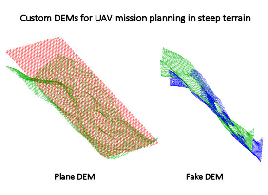
Our goal was to design customized digital elevation models (DEMs) that can optimize mission planning in steep terrain. The custom DEMs modify the actual DTM in a way that allows more consistent UAV distances from the terrain when used for mission planning. This ensures more consistent image overlap, more consistent GSD of images and reduces blind spots. These facts contribute to the efficiency of the dense image matching algorithms used to calculate dense point clouds. The custom DEM also increases flight safety, as uniform distances of the UAV to the terrain prevent the vehicle from colliding with exposed terrain points. To support the UAV mission flying, two custom terrain models and their alternatives have been developed. Additionally, the capturing of oblique images is recommended either instead of or in addition to the conventionally used vertical images.
2. Methodology
2.1. UAV Height, Elevation and Altitude
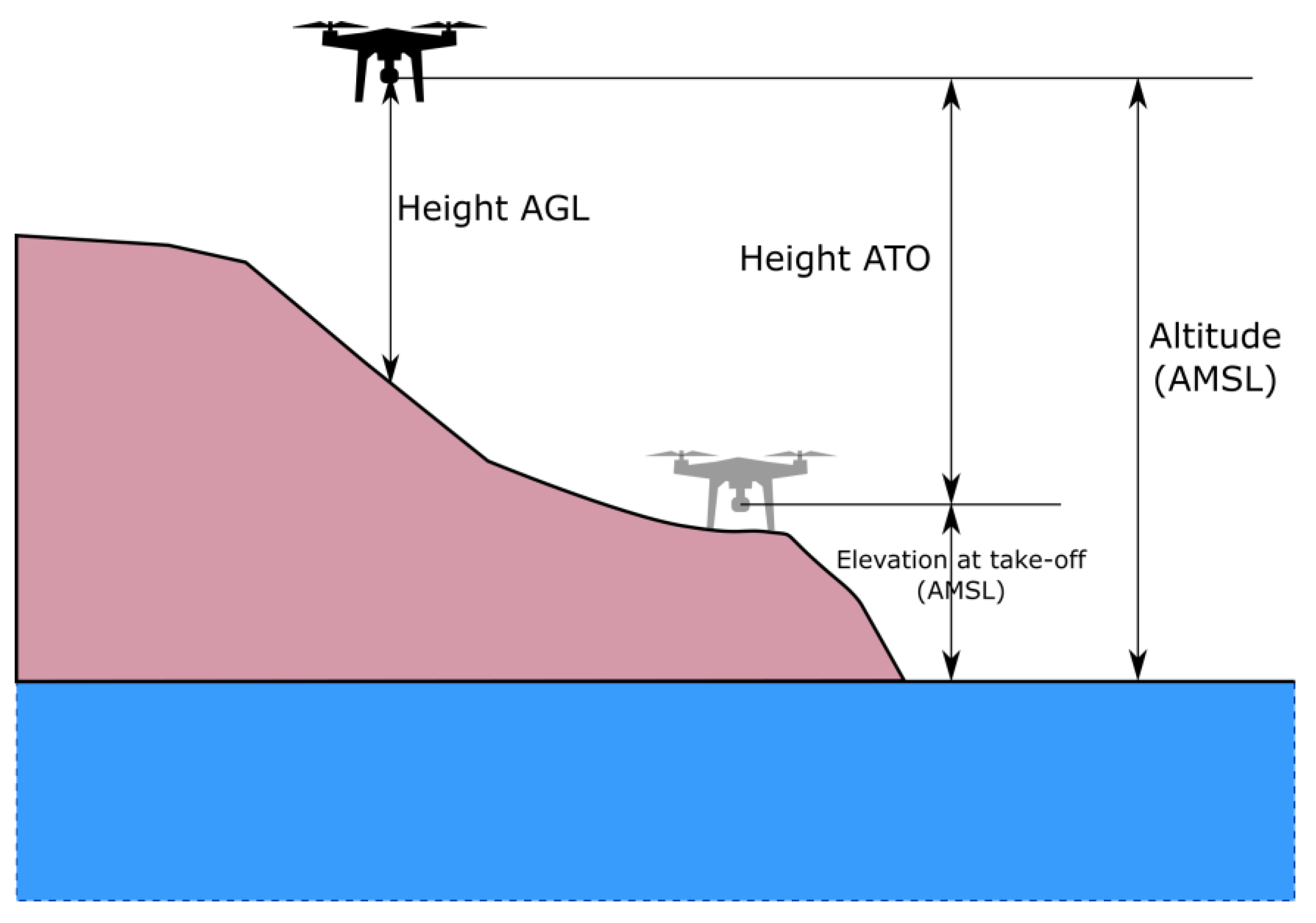
Basic vertical distances of UAV flying are shown in Figure 1. Elevation is the vertical distance of a ground point above mean sea level (AMSL). Altitude is the vertical distance of the current UAV position AMSL. The height above take-off (ATO) is a difference between the altitude and the elevation of the take-off point AMSL. The height AGL refers to the vertical distance between the UAV in flight and the ground. Another important distance is the distance from the projection centre of the camera to ground along the optical axis. When the camera is pointed down in the nadir direction, the distance is equal to the UAV height AGL.
For oblique images, the slant distance from the projection centre of the camera to the ground point in the direction of the optical axis is labeled as DCG (distance camera-ground). Figure 2 shows the DCGs for vertical and oblique images.
2.2. UAV Photogrammetry in Flat and Non-flat Areas
If the terrain is flat or almost flat, the usual method of capturing the terrain with a UAV is to fly horizontally at a certain height ATO, which refers to the vertical distance above the launch point. The camera of the UAV is pointed in the direction of the nadir. The images are taken with a certain overlap to allow 3D reconstruction of the ground using image matching algorithms. Numerous applications, such as Mission Planner, UgCS, DJI GS Pro, 3DSurvey Pilot, Pix4Dcapture and others offer automated mission flying. A flight plan is generated based on a user-defined area, the flight height, overlap of the images and camera type. The plan is uploaded to the UAV, which then takes off automatically, flies to the waypoints, takes images and lands at the home point, provided there are no malfunctions.
If the elevation of the area of interest changes significantly, flying at constant height ATO does not provide optimal image overlap for 3D reconstruction. However, we see the following solutions to the problem:
- A combination of several missions flown at different altitudes,
- Fly the UAV manually or,
- Use a flight planning application that allows terrain following.
The first option, a combination of several missions, is more time-consuming than a single mission, and you must be careful to prevent gaps between the areas flown. Manual flying is even more time consuming, it is difficult to maintain the same height AGL, and there is no guarantee of correct image overlap. If an adequate terrain model is available, an autonomous flight mission following the terrain is the best option.
A digital terrain model (DTM) is required to enable the UAV to follow the non-flat terrain. DTMs or DEMs with a certain spatial resolution can be provided worldwide (mostly in low resolution), nationwide (mostly in different resolutions) and locally from previous surveys. The biggest problem is the lack of software that supports terrain data for mission planning. At the time of our survey flights (end of 2018), we found a single application for DJI UAVs with DTM import capabilities, namely Drone Harmony. According to [7] from 2019, UgCS was the only other commercial application that offered such possibilities at that time.
2.3. Basic aspects of UAV Photogrammetry in Steep Terrain
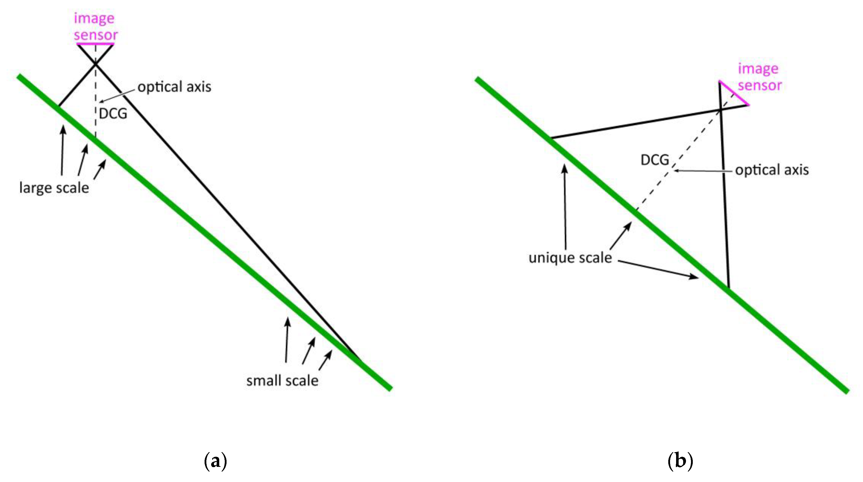
An important aspect of UAV photogrammetry in steep terrain is the direction of the optical axis of the camera. The image scale in aerial surveying is based on the ratio between the distance from the image element to the projection centre and the distance from the projection centre to the object on the terrain. When the optical axis of the camera was directed vertically to the ground, as is common in flat areas, the image scale of steep terrain changed significantly. In these cases, the oblique images, whose optical axes were perpendicular to the ground surface, provided much better image properties with respect to the image scale and the subsequent image GSD. Figure 2 displays the geometric comparison between the vertical image and the oblique image perpendicular to the terrain.
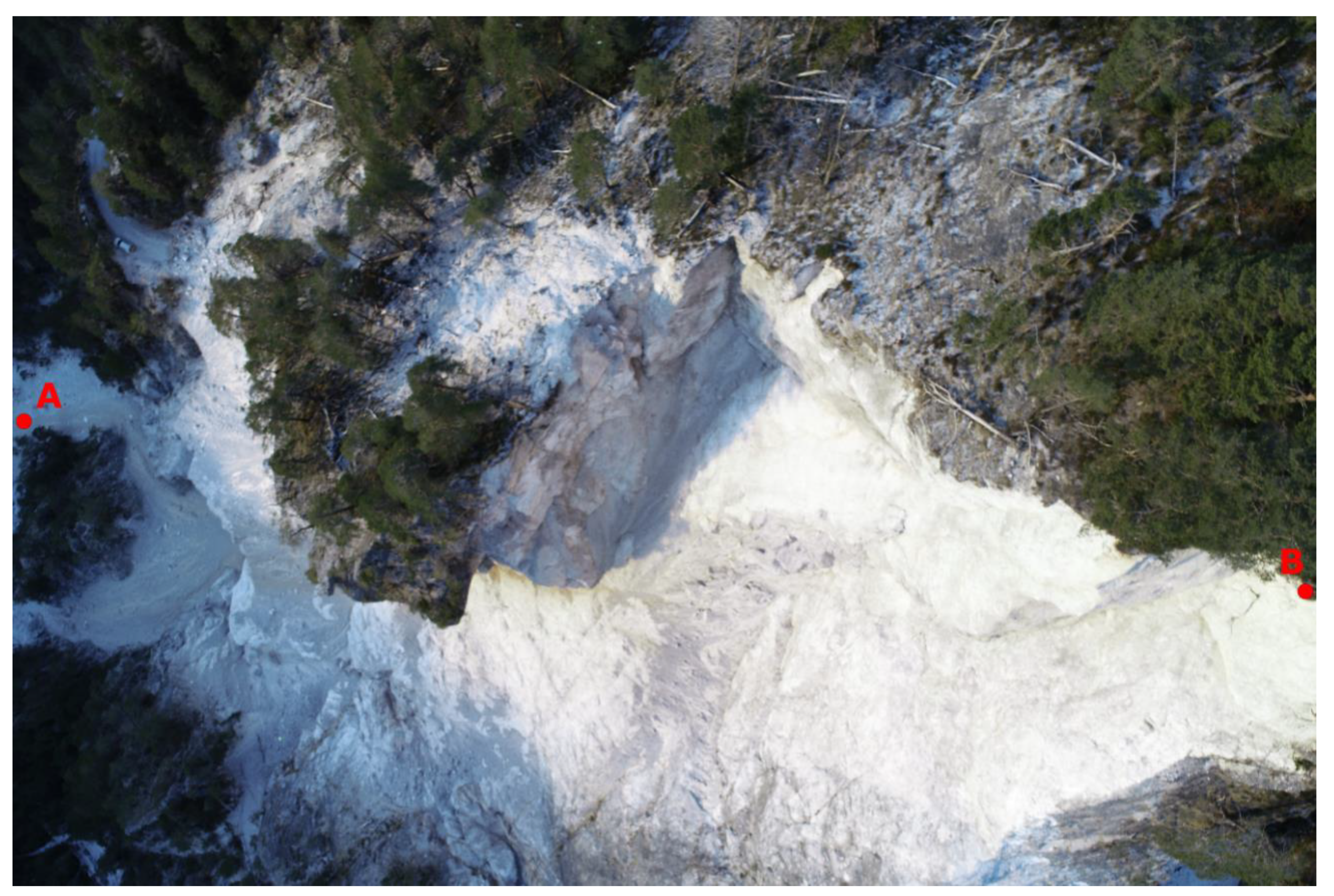
An example of an extreme situation on a vertical image in steep terrain is shown in Figure 3. The height differences from the image projection centre to points A and B were 288.4 and 19.6 meters, respectively. The 3D distances to the same points were 362.0 and 53.7 meters.
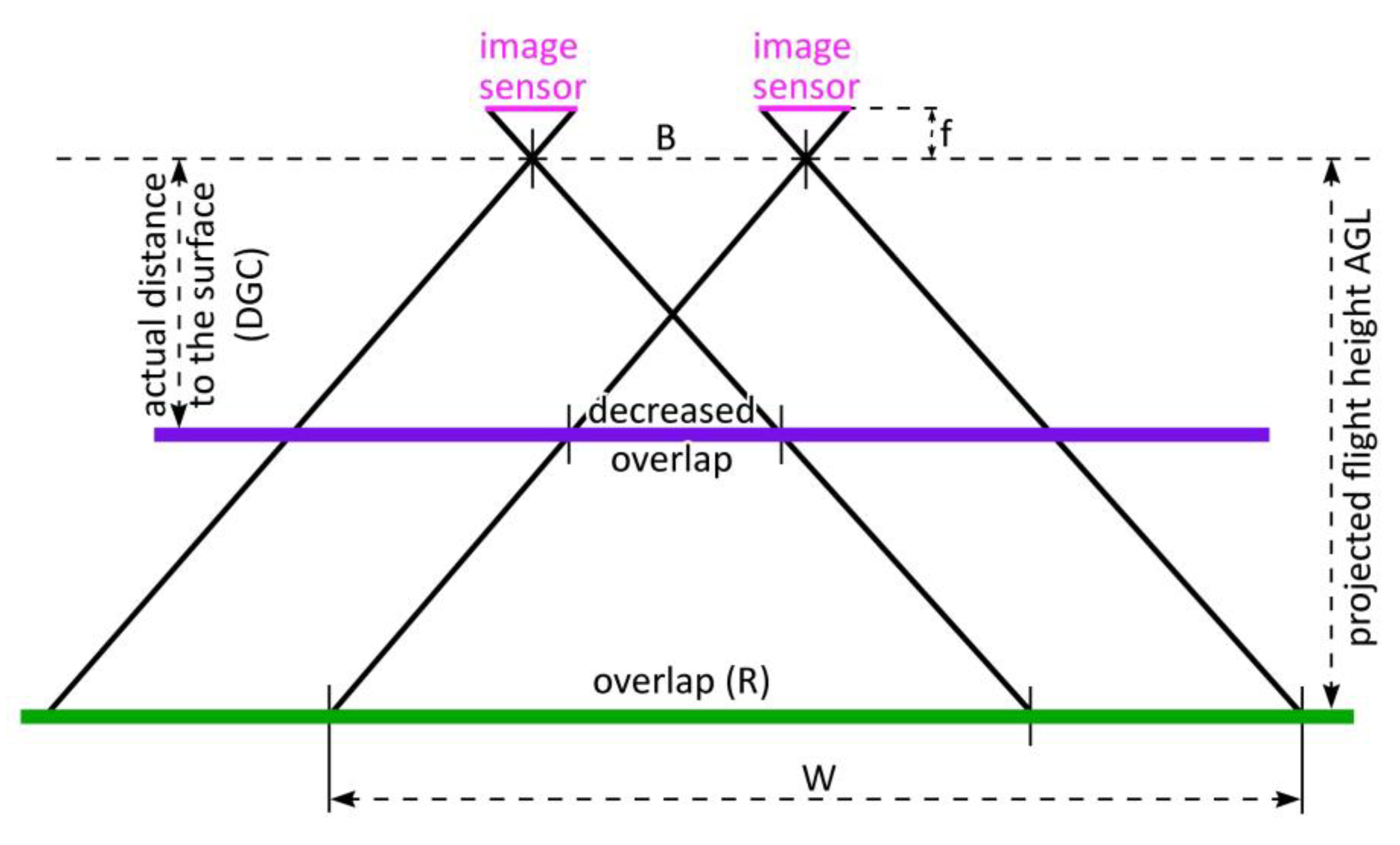
Since the image overlap is calculated according to the planned UAV height AGL, there is an issue in vertical images because the distance to the upper part of the captured area in the image is much shorter than the height AGL. In Figure 3, point B was only 19.6 meters below and 53.7 meters away from the UAV, whose projected height above the DTM was 80 meters. As a result, the overlap was reduced and could become critically low in very steep areas. The situation is depicted in Figure 4 for vertical images and horizontal flat terrain. Equation (1) provides the relationships between the overlap fraction (R), the image base (B) and the dimensions of the image sensor scaled to the ground (W) [23]:
The image base was calculated from the specified height AGL and the projected overlap. With a constant image base, the overlap was reduced to 60% at the half of the height AGL and further reduced to 20% for a quarter of the height AGL.
2.4. Development of Custom DEMs
The creation of custom DEMs is applicable to any publicly available DTM. In our experience, we advise against using the global SRTM (shuttle radar topography mission) DEM. Due to its spatial resolution of 3 arcseconds, the SRTM DEM is not accurate enough to plan a UAV mission in steep hilly terrain [9,24,25,26]. The national 5-meter DTM (NDTM) of The Surveying and Mapping Authority of Slovenia was selected for the study.
2.4.1. The Plane DEM
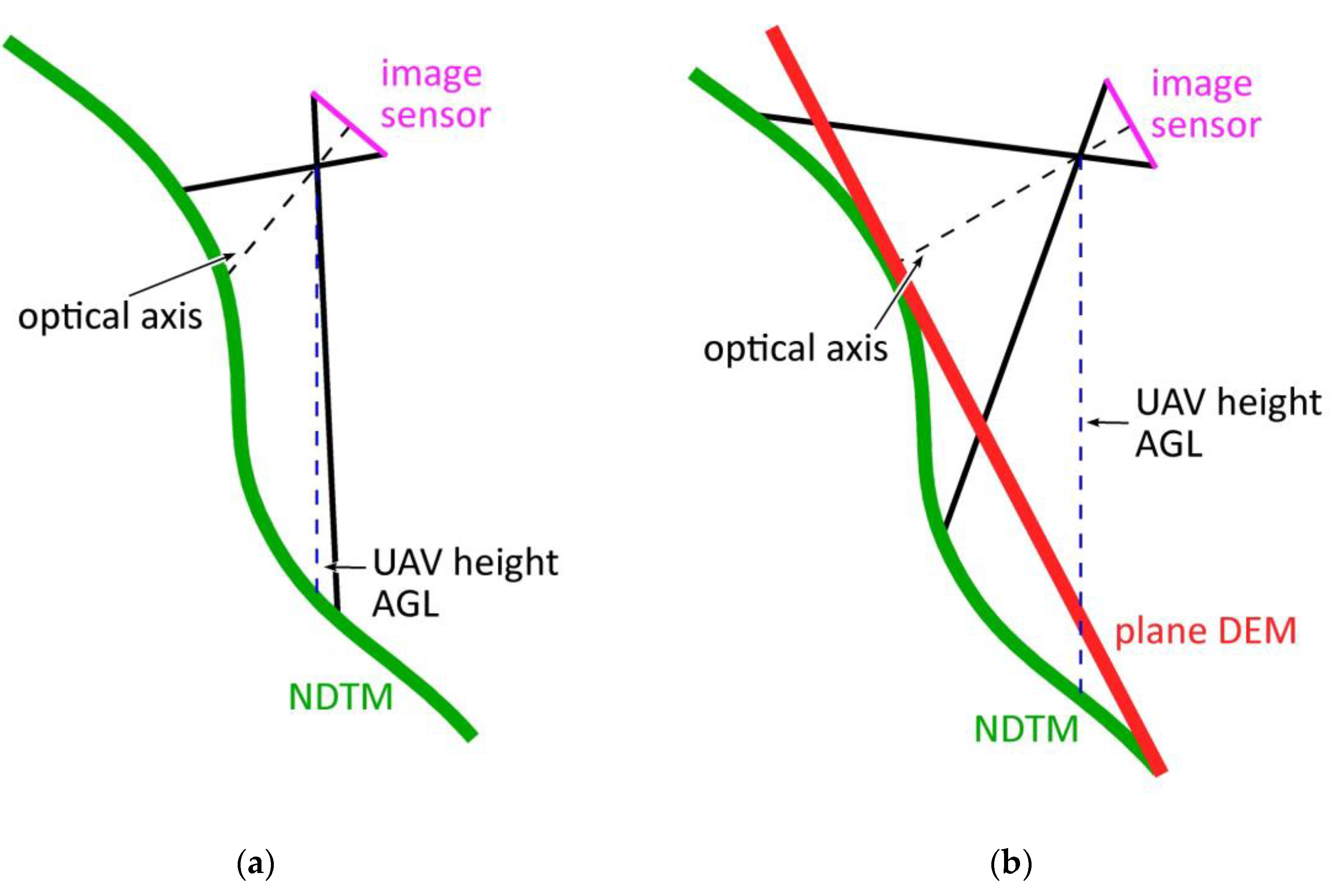
To prevent the UAV from getting too close to an area that suddenly became very steep—since the UAV height AGL is the vertical distance from the imported NDTM, see Figure 5a—the idea was born to create a plane surface over the extreme parts of the area. Consequently, the distance of the UAV from the terrain was much more favorable, as shown in Figure 5b.
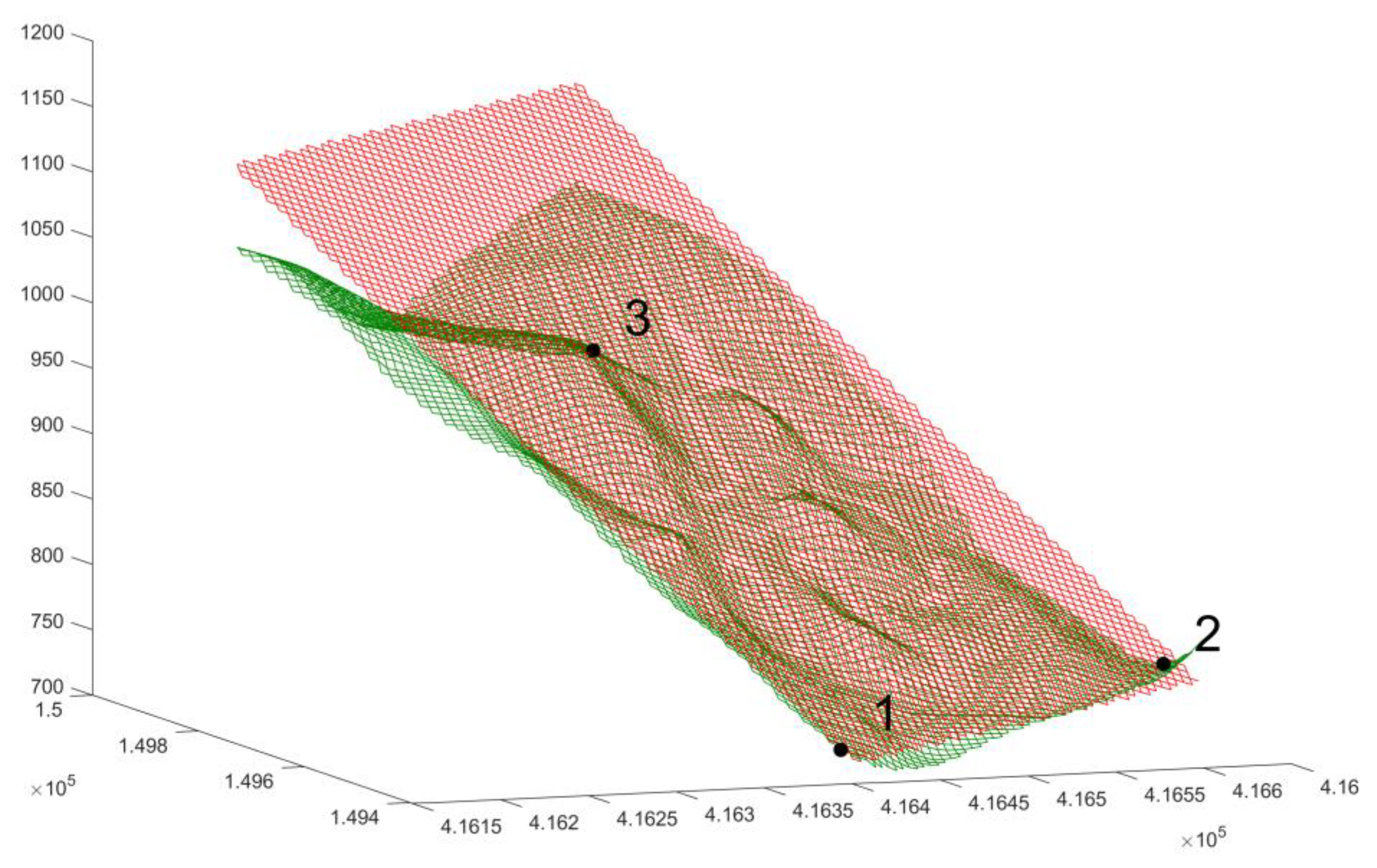
Figure 6 displays the plane DEM set above the NDTM. Three reference points were selected for the calculation of the plane. Two reference points, marked 1 and 2 in Figure 6, were located in the lowest part of the NDTM, and point 3 was the one where the plane through points 1 and 2 touched the NDTM as it approached the NDTM from the vertical position. The reference XY coordinates of the plane DEM were the same as for the NDTM, only the elevations were recalculated. Therefore the resolution of the plane DEM was the same as for the NDTM.
This DEM ensures a certain minimum distance to the terrain. Furthermore, an appropriate overlap was ensured. The disadvantage is the greater distance to some areas, e.g., local depressions, which leads to a lower model resolution of them.
2.4.2. The Fake DEM
The plane DEM is a simple surface that is easy to calculate because only three reference points are needed. However, this simplicity has some shortcomings. The differences in elevations between the plane DEM and the DTM can become large. Therefore another custom DEM was developed.
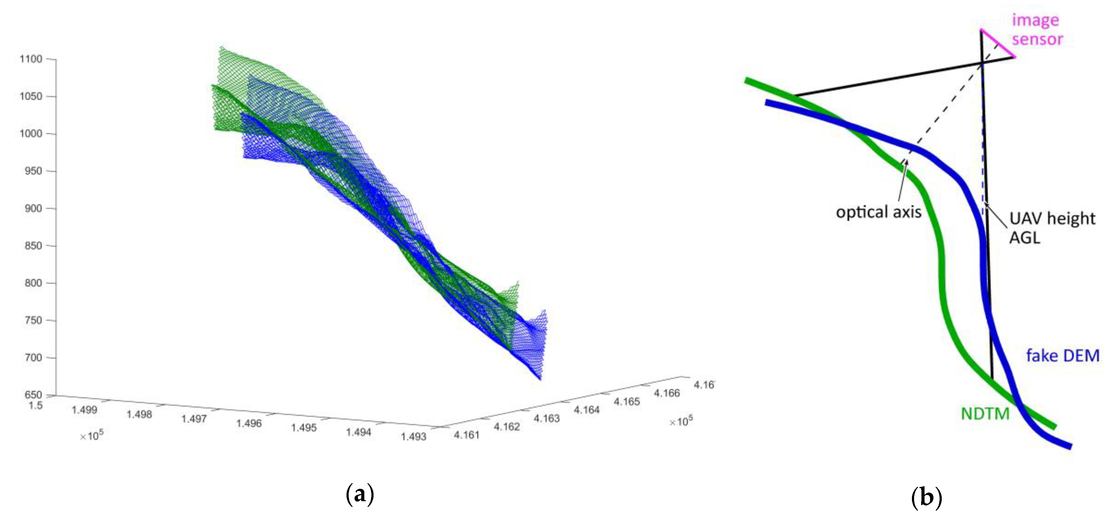
The fake DEM is specially designed for UAV surveying with oblique images. The fake DEM grid is shifted to the NDTM grid so that the DCG to the NDTM is constant at given values of the projected height above the fake DEM, UAV heading and gimbal angle, all of which are constant during a flying mission. The recalculated grid points and their elevations form the fake DEM. A graphical relationship between the fake DEM and the NDTM is shown in Figure 7.
2.4.3. The tilted DEMs
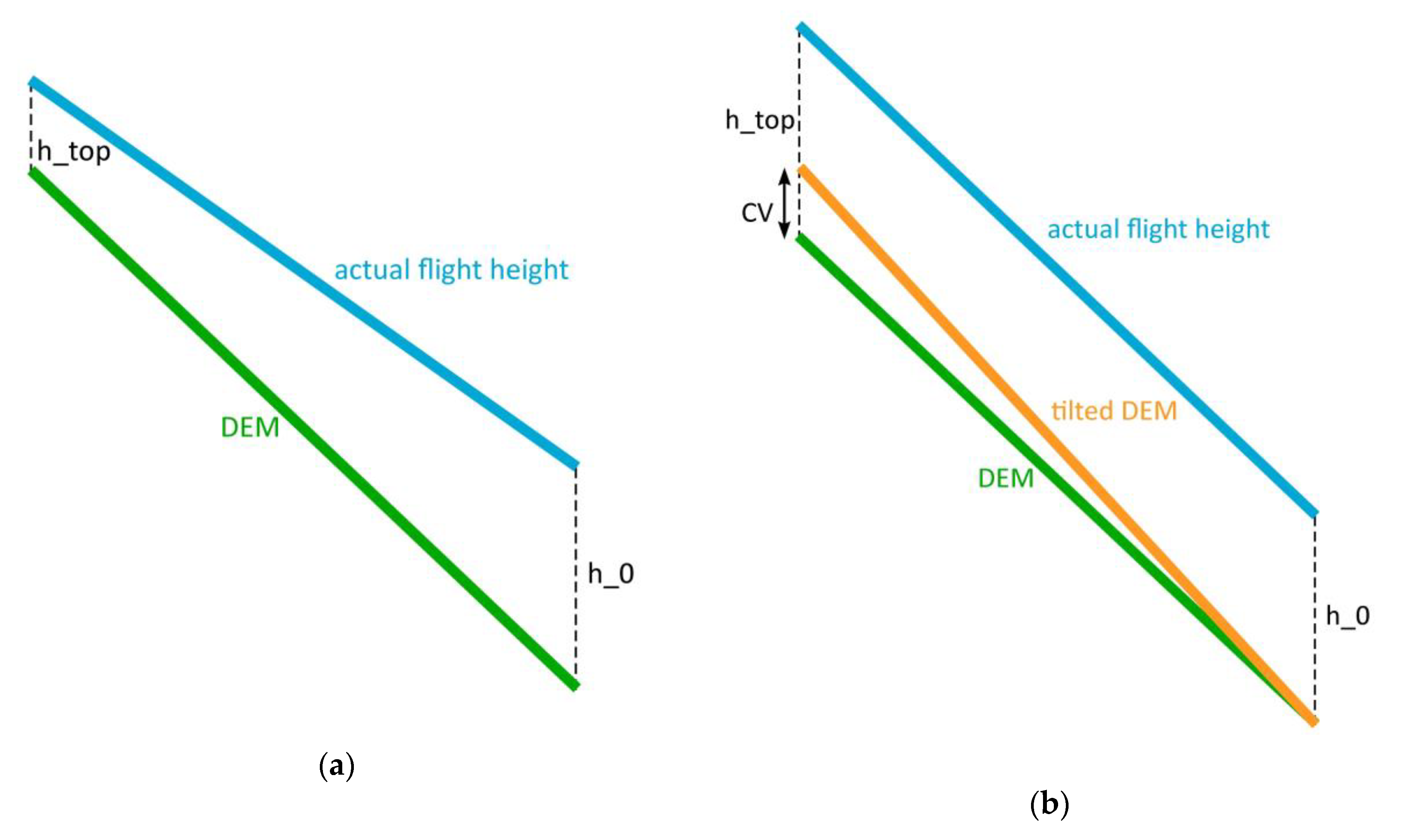
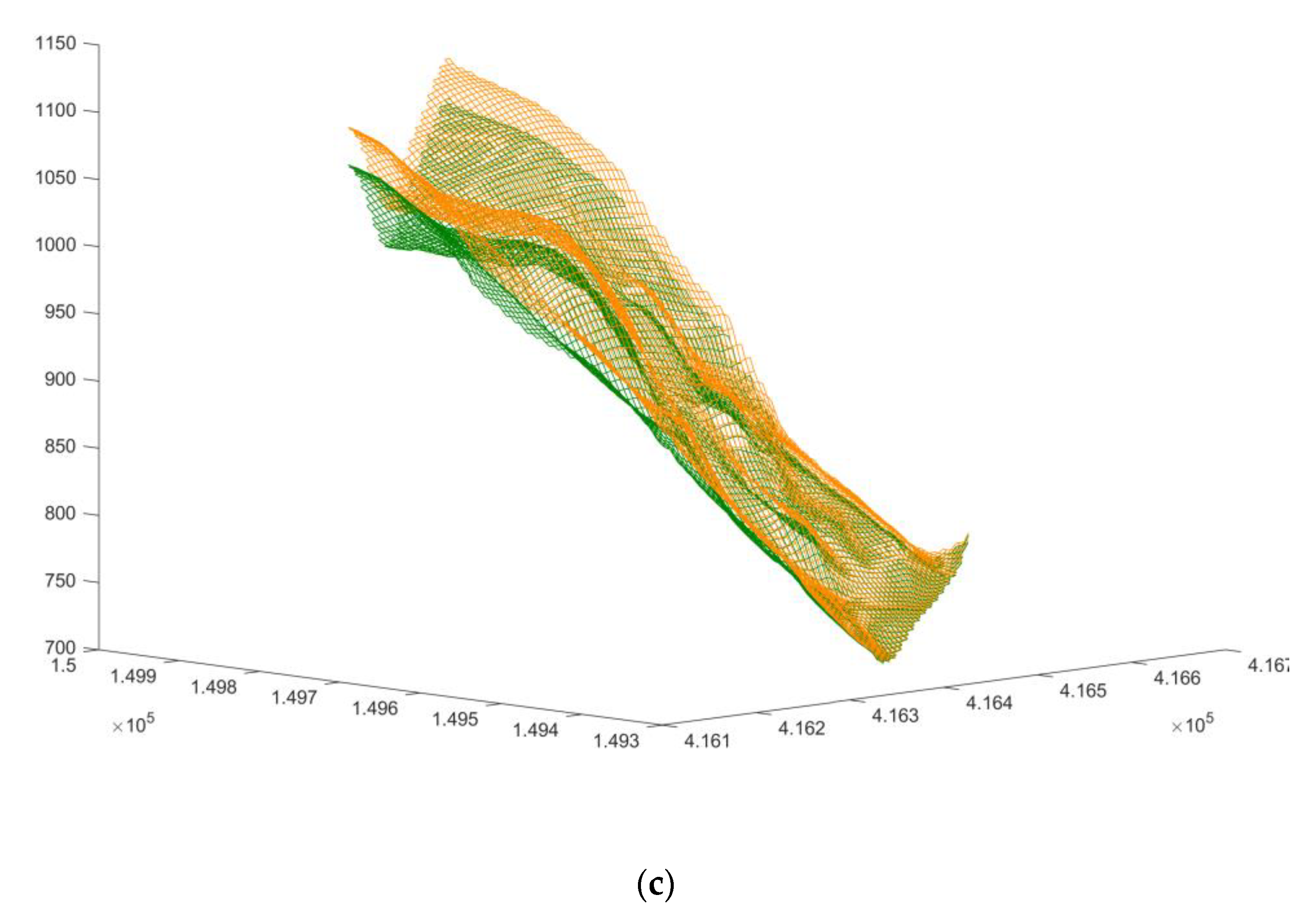
An unexpected UAV's behavior was observed during its practical deployment in a mountainous terrain. As the UAV height ATO increased, the height AGL decreased. A generalized situation is shown in Figure 8a. The UAV starts the survey at the projected height AGL h_0. The height AGL at the top, denoted h_top, should be similar to h_0. However, in our case study, which is described in Section 3, it was not, since h_top was in all cases about 20 meters smaller than h_0. To compensate for the error, the tilted DEMs were introduced. The idea is to tilt a DEM so that the actual flight height is more parallel to the basic DEM and h_top is similar to h_0. The situation is shown in Figure 8b. The compensation value (CV) has been set at 30 meters, to be on the safe side. The tilted DEMs were recalculated DEMs so that the elevation increased linearly from 0 at the bottom to 30 meters at the top. The tilted values were applied to the NDTM, the plane DEM and the fake DEM. Figure 8c displays an example of a 3D comparison of NDTM and the tilted NDTM.
3. Site Description, Field Work and Data Processing
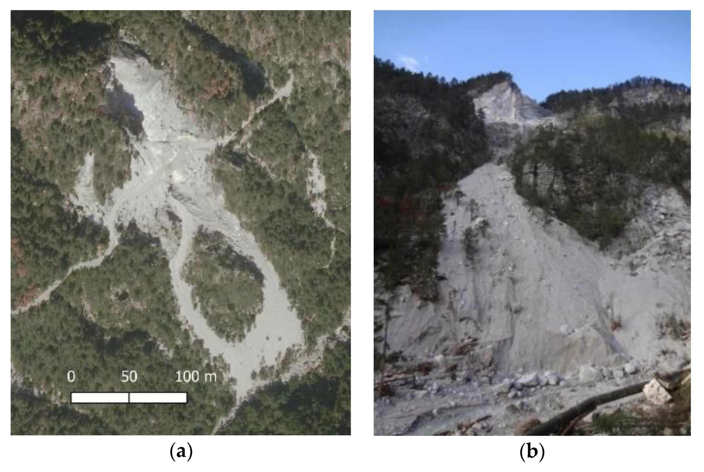
The developed DEMs (plane, fake, tilted plane, tilted fake and tilted NDTM) and terrain-following aerial surveys were tested on the Belca active rockfall in the NW part of Slovenia. It lies only a few 100 m above the village of Belca, while a sawmill is located just below the unstable slopes. In 1953 a large rockfall event with considerable damage was reported in this area. A forest road crossing the area is shown in Figure 9a. The next major rockfall event in February 2018 triggered the debris flow that accumulated on the road that has been closed since then. Another massive rockfall event occurred in October 2018, eroding the left bank of the Belca torrent in addition to the material on the rockfall area. The debris has accumulated in and around the Belca river bed. It has largely damaged the smaller hydroelectric power station and the local sawmill. Thereafter, some cracks in the rock mass near the top of the slide caused concern, so that a controlled removal of the threatening block with explosives was initiated. The rockfall extends over an area of about 100 m × 300 m and spreads between elevations 710 m AMSL at the toe and 1020 m AMSL at the crown.
In the period from November to December 2018, several UAV surveys were carried out in which different DEMs and types of images were tested. Table 1 shows an overview of the surveys.
The UAV height AGL dictates the GSD of the images. The DJI Phantom 4 Pro used in research achieved a GSD of 1 cm at a height of 36.5 m, 2 cm at a height of 73 m, etc.
The NDTM was geolocated in the plane coordinate system in XYZ format. For use with the Drone Harmony app, it must be transformed into WGS-84 and then exported in Esri ASCII format. The NDTM was initially used for vertical and oblique image acquisition. For the latter, the gimbal pitch was set to -45 degrees, as the average slope angle is close to 45 degrees. The planned height AGL for all flights was set at 80 meters. The front overlap was set to 80% and a side overlap at 65%. As already mentioned in Section 2.3, the image overlap is reduced in steep terrain. To keep the actual overlap at the desired rate, the projected overlap can be set higher, but this would mean more images and longer flight times. In order to facilitate the comparison of the two sets of images (vertical and oblique), it was decided to keep the same projected heights and overlaps.
Since the topography of the area is diverse and the slope angle changes rapidly, the NDTM was considered unsuitable for oblique imagery. Two user-defined DEMs were created to support the acquisition of the oblique images.
The plane DEM was generated in the national coordinate system and transformed into WGS84 and Esri ASCII format, same as for the NDTM. The steepest inclination of the plane DEM was 43.9 degrees with an azimuth of 332 degrees. Since the surface of the plane DEM differs from the NDTM, the GSD on the NDTM varies when the plane DEM was used in mission planning.
For the fake DEM of the Belca case, the elevations of the DTM were recalculated in such a way that from any point 80 meters above the DEM, the DCG at the pitch angle -45 degrees and heading 330 degrees was 60 meters. In practical use, the fake DEM was uploaded to the mission control app, the flight height AGL was set to 80 meters, the gimbal pitch angle to -45 degrees and the heading to 330 degrees. The DCG to the NDTM terrain was 60 meters. The value of 60 meters was a rounded value of 80 m × cos (45°) = 56.6 m, where 45° was the pitch angle.
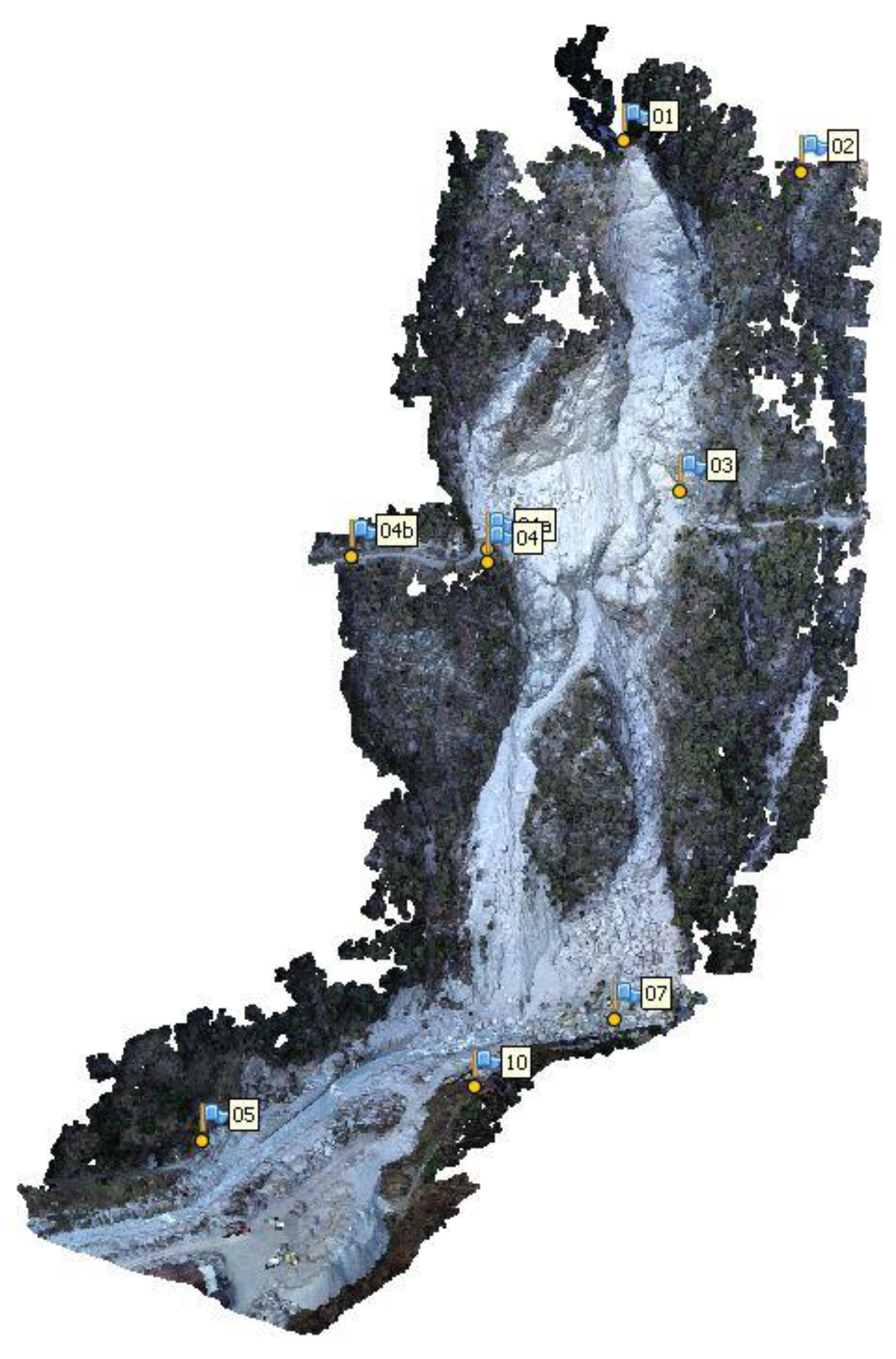
The georeferencing of the UAV images was performed using ground control points (GCPs), which were signaled with targets (a black circle 27 cm in diameter on a white background). Ideally, the GCPs should be evenly distributed over a surveyed area [27,28,29] to achieve optimal accuracy of results. The terrain of the Belca rockfall is not only steep, but it is also a challenge to reach some areas in order to set the GCPs optimally. Figure 10 shows the geometric distribution of the GCPs. In the middle of the area, in this case in the central part of the rockfall, there should be some GCPs. Firstly, it is very dangerous to cross the rocky area and secondly, it would be difficult to fix a GCP target on the unstable ground. Since some of the targets were set under adverse GNSS conditions, we used two different GNSS receivers and two modes, RTK and fast-static, to achieve high quality results. The acquired accuracy of the GCP positions was about 5 cm. The GCP coordinates were determined in the national reference coordinate system D96/TM (EPSG: 3794).
The images were processed with Agisoft Metashape software [30]. The images' exterior orientations, calculated during the bundle block adjustment (BBA) were used to analyze the distances of the UAV from the ground. Together with the BBA, dense point clouds and orthophotos were created to visually evaluate the effects of various flight missions on the final products.
4. Results
This section presents the main height-related results of the Belca case study, which used custom DEMs that would ensure a constant distance between the UAV and the terrain in a vertical or oblique direction. The practical aspects of vertical and oblique images were discussed in Section 5.2.
4.1. UAV heights over NDTM and custom DEMs
DJI's technical support would not reveal to us the principles behind the estimation of aircraft height. Based on information collected in the forum on the DJI website and [31], DJI's non-RTK aircraft operate with relative heights, using the on-board barometric altimeter and height 0 being the point at which the UAV takes off from the ground.
When using the terrain file in Drone Harmony Pro application, it is necessary to select the starting point, as the height at this point is set to 0. According to [31] the mission planning procedure creates a grid over the user selected polygon. Each grid point height was calculated as a weighted average over the adjacent DTM grid points.
In Figure 11, Figure 12, Figure 13, Figure 14 and Figure 15, the UAV height ATO refers to the barometric height of the UAV at the time an image is taken. The height AGL was calculated as the height ATO, reduced by the interpolated elevation value of a DEM at the point vertically below the projection centre (PC) of an image. The barometric height ATO was taken from the flight log. The coordinates of PCs for all images were estimated in the bundle adjustment during the SfM. The DCGs to DEMs were analyzed either in the vertical direction or in the slant direction of the optical axis.
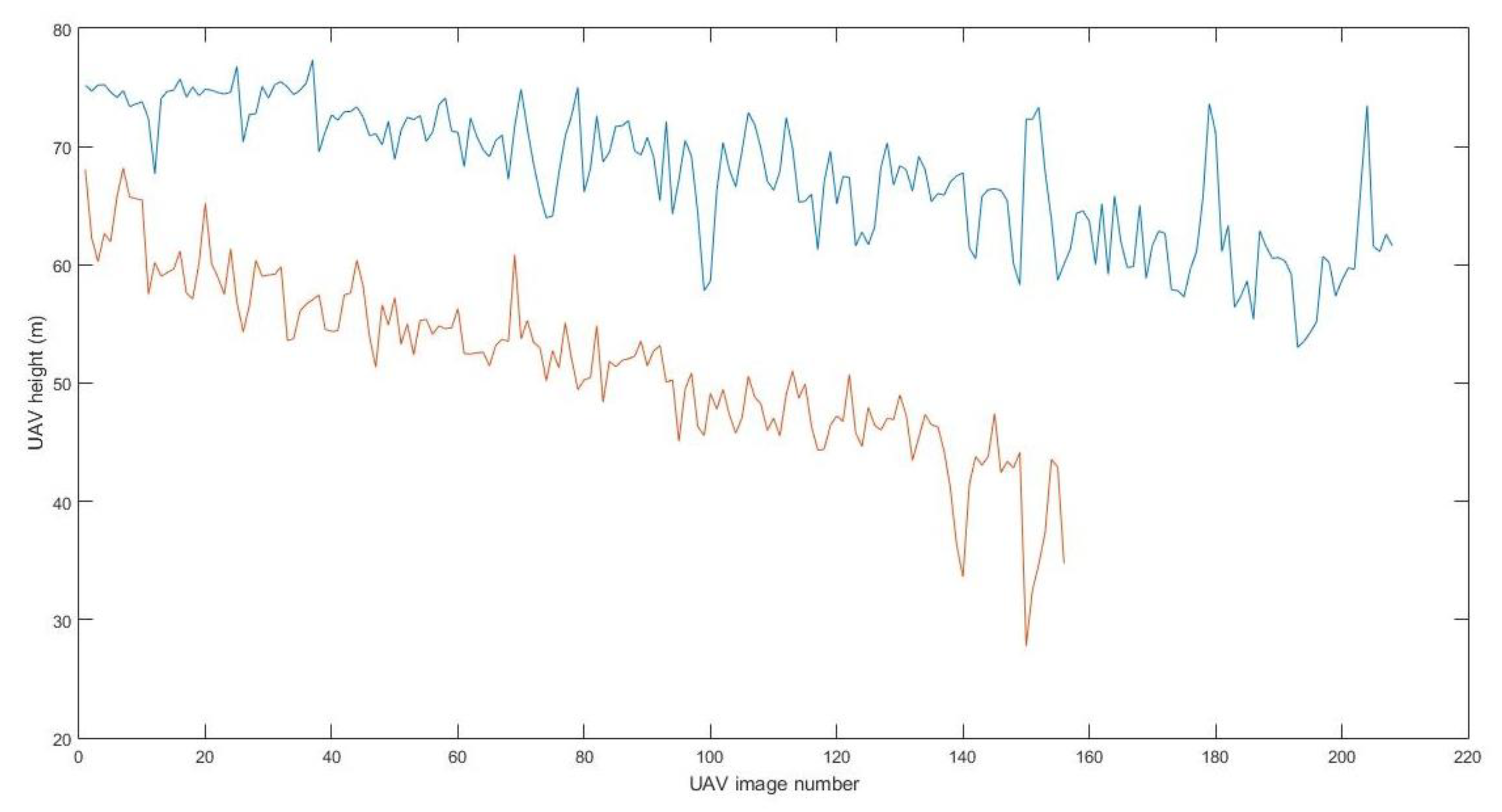
Figure 11 shows the UAV heights above the NDTM using NDTM or custom DEM in mission planning. When using NDTM, some of the spikes could be caused by NDTM smoothing in the mission planning application. Since the surface of the plane DEM is smooth by itself, sudden changes in height are smaller than when using the NDTM for mission planning.
The flight heights of the same plane DEM based flight over the plane DEM are shown in Figure 12a. The corresponding image block is shown in Figure 12b. The first spike (around image number 140) was a consequence of the PC heights of the images named 297-300, which should be almost equal, but the UAV descended 12 meters in between. The last spike was located between the images named 310 and 311. The difference in height should be more than 15 meters, but the actual lift was only 4.5 meters.
The height of the UAV above a certain DEM should remain constant throughout the mission. Ideally, this height should be 80 meters, as it was planned for all flights. Due to unknown inconsistencies of the initial height ATO the starting height deviated from 80 meters. However, the following heights AGL should be close to the initial height. The cases presented differ from the expected ones because the height AGL decreased steadily with increasing amount of the height ATO. All other flights of the first two days show the same trend.
Even though the DCGs are only relevant for the actual terrain represented by the NDTM, the example in Figure 12 is presented to further strengthen the hypothesis that the barometric height AGL of the UAV differed from the actual height AGL.
To investigate the issue, the PCs' heights ATO of one flight were compared with the barometric heights ATO of the UAV of the same flight. The adjusted PC positions can be considered as the true positions. The comparison is depicted in Figure 13. The deviation increased to about 20 meters at the largest heights ATO, which was consistent with the cases shown above.
The flights were carried out under different weather conditions. Most of the flights were from bottom to top, some also from top to bottom. The height difference at the top was always in the range of 15-25 meters, so that it can be considered a systematic error.
4.2. Tilted DEMs
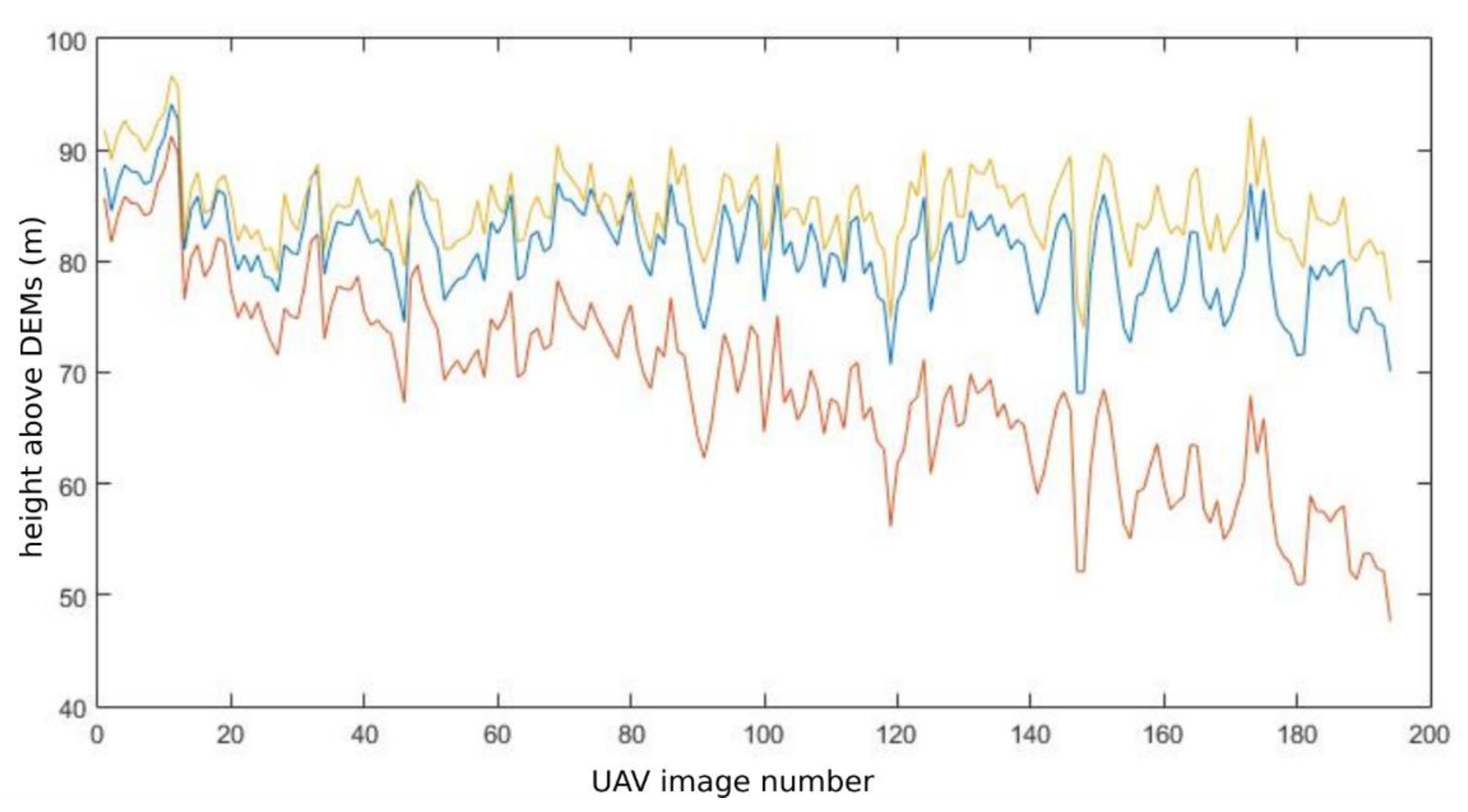
To solve the issue, the tilted DEMs were developed, see Section 2.4. As an example, the heights above the fake DEM and the tilted fake DEM are shown in Figure 14. The actual height above the DEM decreased again as the height ATO increased. However, the heights above the original fake DEM were much more constant. For comparison, the barometric heights of the UAV are shown.
If the tilted DEMs were used for mission planning, the actual heights AGL were much more constant, as can be clearly seen in Figure 14 (see blue line).
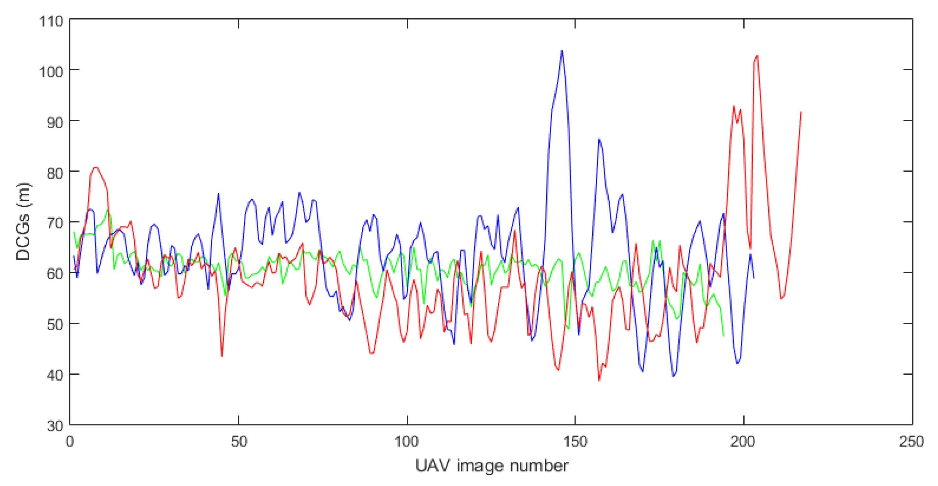
Moreover, when using oblique images, the DCGs along the optical axis were more important than the actual flight heights AGL. The DCGs of all three missions on the third day to the actual terrain represented by the NDTM are shown in Figure 15.
The DCGs from the tilted fake DEM mission are the most constant, ranging from 47 to 72 meters. As a reminder, the fake DEM was designed so that the DCGs are at least theoretically 60 meters long.
5. Discussion
5.1. UAV over-Terrain Flying in Steep Terrain
To execute a terrain-following mission survey, a special software application and a DEM are required. When flying in steep terrain, the flight planning software must allow the user to import an accurate terrain description [7]. We used Drone Harmony application as one of the few that were able to import a DEM for a DJI-made UAV at the time of our surveys.
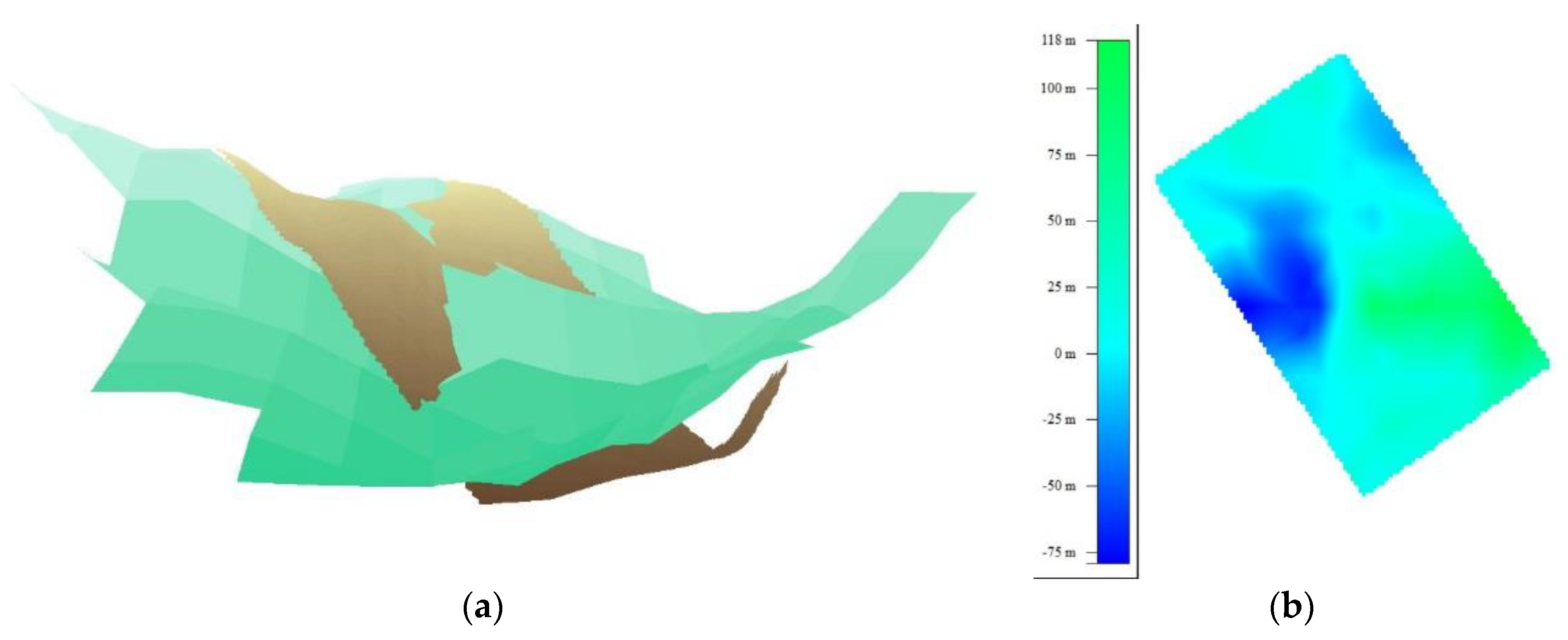
Figure 16 shows the comparison between the SRTM DEM and the NDTM. Since the SRTM DEM generalizes the terrain due to the low resolution, it is clear that the SRTM DEM cannot be used for UAV missions in steep hilly terrain. It could even become dangerous if the aircraft follows the SRTM terrain, because it could crash to the ground. The SRTM DEM was more than 75 m below the ground at some spots of our test area, see Figure 16b. The authors of [9] also claim that the global DTMs may not be able to provide sufficient accuracy in the estimation of height AGL.
5.2. Vertical and Oblique Images in Steep Terrain
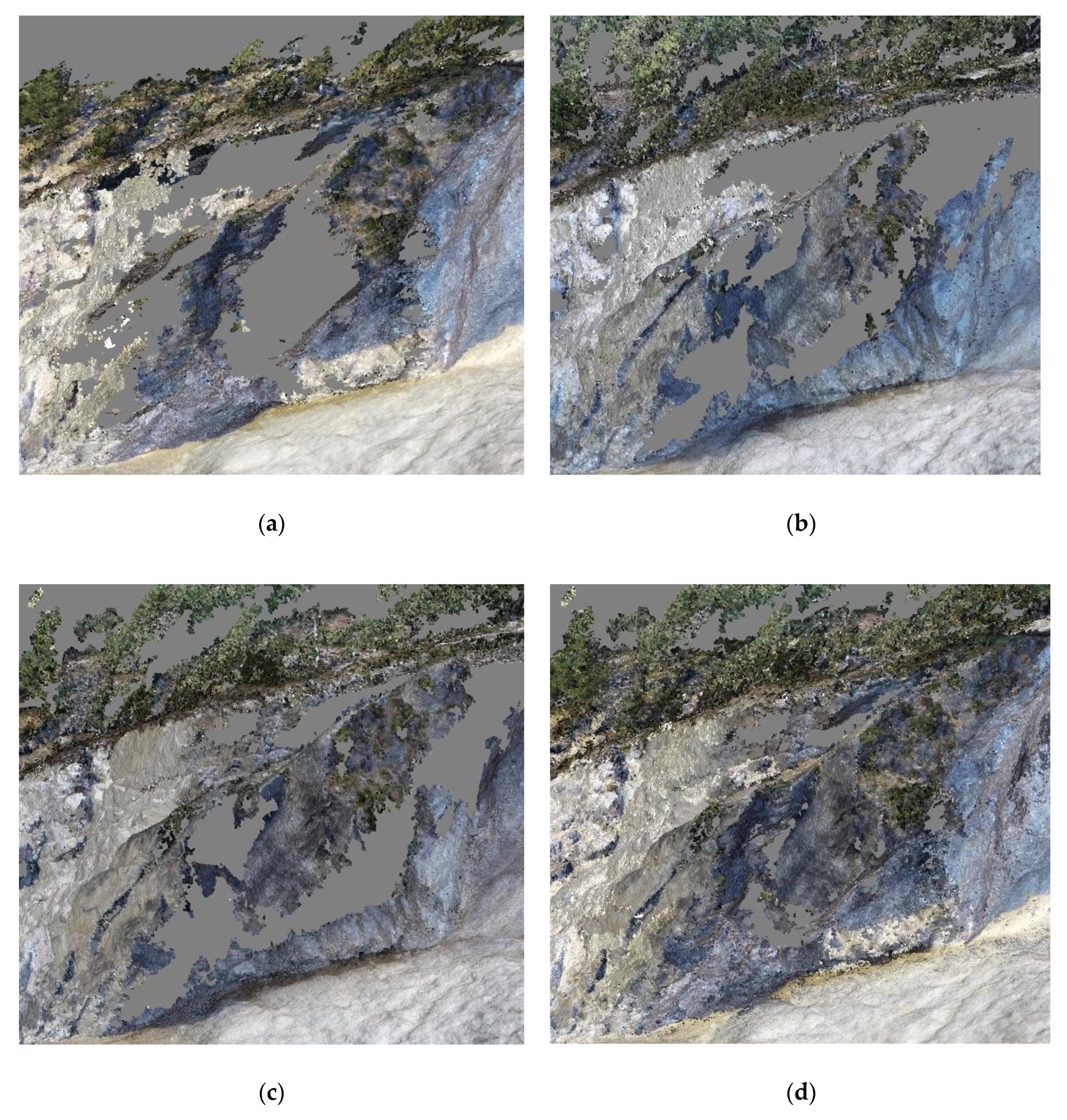
The use of oblique images is particularly appropriate in hilly terrain with rugged topography and overhangs, as shown in Figure 17. The images in Figure 17a–c show dense point clouds from single surveys, while Figure 17d displays a merged point cloud from the vertical images and the oblique images taken on the plane DEM. If only the vertical images are used, many topographic details may be lost, as shown in Figure 17a. With the use of the oblique images and the combination of vertical and oblique images, see Figure 17d, the result may still not be perfect, but there is much less void space and the terrain modeling is more accurate. Rossi et al. [32] confirmed that the use of aerial nadir view is not very suitable for surveying subvertical walls. On the other hand, the contribution of oblique images increases the consistency of the reconstructed surfaces. Tadia et al. [33] improved the vertical accuracy of the photogrammetric model when they included oblique images within their nadiral dataset. Similarly, the authors of [34] state that the use of a tilted camera improves the robustness of the geometrical model. The use of oblique images is crucial to improve the density of the point cloud, especially in connection to peculiar features of the surveyed object [35].
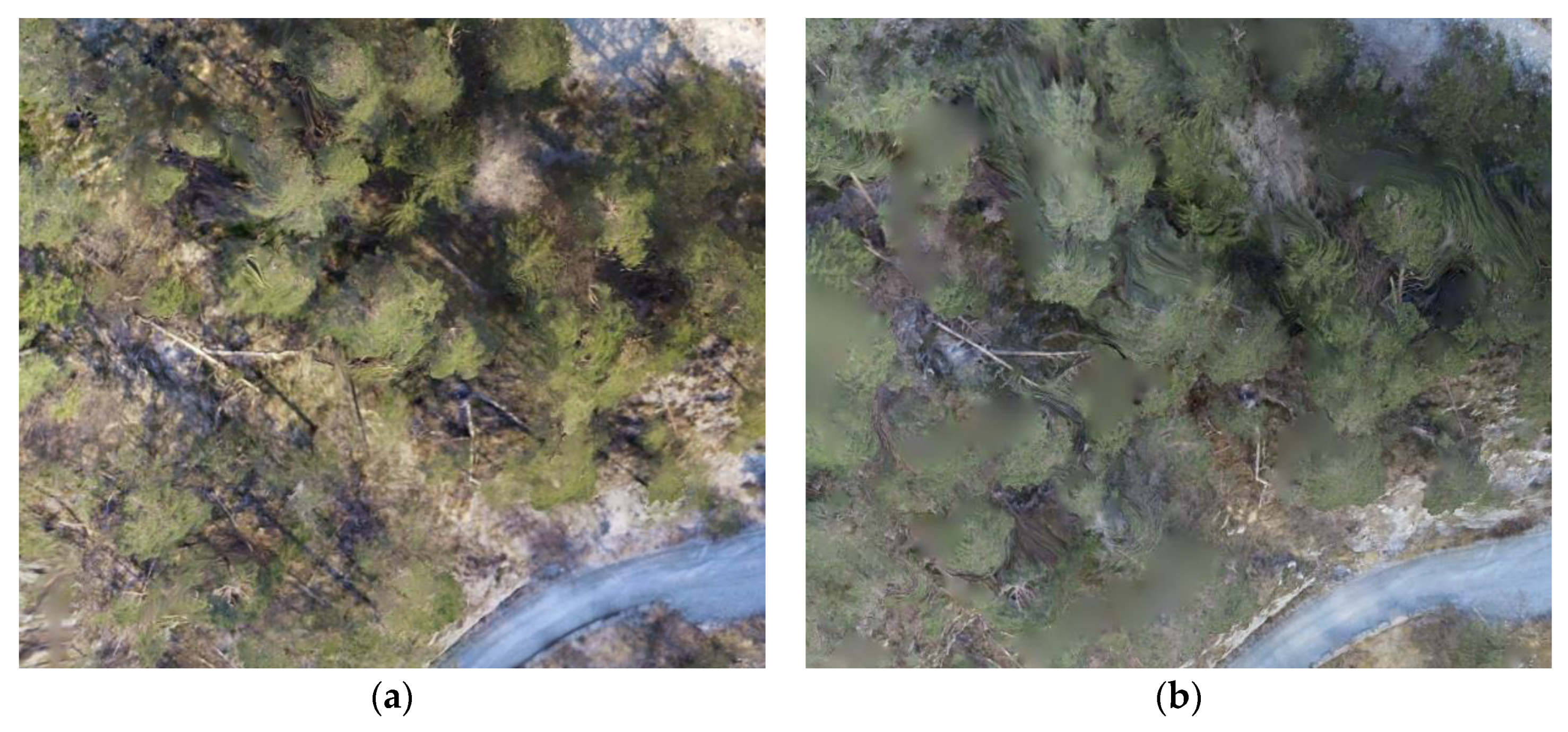
There are also some issues with the oblique images. If any objects with significant height above the ground are present (e.g., vegetation), they could cause a disturbance in imaging because they are captured from the side, not from above as in the vertical imagery. As a result, it is very difficult to generate an orthophoto from the oblique images if such is required. Vertical images are more appropriate to produce orthophotos [36]. As an example, Figure 18 shows two inserts of orthophotos of a forest area next to the rockfall. It is very obvious that the software has problems to create a clear orthophoto from the oblique images. Amrullah et al. [37] suggested that only vertical images should be used to produce orthophotos.
The main problem with vertical images in steep terrain is the large difference in scale in a single image, see Figure 2, Figure 3 and Figure 4, which probably causes longer processing times. Not only the scale is an issue, a big factor is the appearance of a detail in many images. For example, a detail in the lower part of the rockfall appears in more than 100 vertical images. The number of oblique images with the same detail was about 10. In figures, a dense cloud generation from 218 vertical images took 10 hours and 54 minutes and 78.3 million points were calculated. A dense cloud calculation from 203 oblique images took 1 hour and 24 minutes, in which 129.8 million points were calculated.
5.3. Height Decrease
An unexpected issue occurred on all our flights, namely the decrease of the actual height of the UAV above any DEM as the height ATO increased. At a total height of about 300 meters ATO, the actual height AGL decreased by about 20-25 meters at the top. We were able to compensate for this by tilting the DEMs upwards, see Section 2.4.3. These values applied to the Belca site. This issue needs to be further investigated at other sites at different elevations.
6. Conclusions
The execution of a UAV mission in steep terrain is much more complex than in flat terrain. In the latter, the UAV flies at a constant height ATO and the images are captured vertically. In non-flat terrain, the UAV must follow the terrain at a certain height AGL. Mission flying in steep terrain is much more comfortable than manual flying, mainly because of the changing elevation of the terrain, but still special care is needed during preparation and even more during the flights. In addition to the terrain itself, high trees or other tall objects need to be taken into account when setting the flight height.
To be able to follow the terrain, a DEM with a suitable resolution and topographical accuracy is required. Using low resolution global DEMs, such as SRTM, is not only inadequate, but can also be dangerous. Based on our research, a 5-meter NDTM contained sufficient topographic detail to adequately follow the terrain from a UAV height of 80 meters. A special application is required for the use of a DEM for terrain-following flying.
A UAV survey of a steep terrain should not contain only vertical images, because there are large scale changes in the images and not all details are captured in the rugged terrain. The processing time of the vertical images is much longer than the processing of the oblique images. The oblique imagery also has an issue generating an orthophoto image.
To overcome the problems mentioned above, the optimal solution is to use a combination of vertical and oblique images. It is true that the combination of both types of images requires even more processing time, but the result is a point cloud with much more detail, and a proper orthophoto can be produced.
Regular DTMs as a basis for the terrain following flying are only suitable for the vertical images. Custom DEMs can be generated to create a surface for the oblique images. The plane DEM is easy to construct, it assures the minimum distance to the surface and thus a sufficient overlap. However, the fake DEM is preferred, as the DCGs are preserved and thus the GSD is kept constant.
If due to limited time or UAV batteries only one flight mission can be performed and the orthophoto is not required, we recommend the use of the fake DEM and oblique images. For the optimal complete solution, select NDTM for the vertical images and the fake DEM for the oblique images. If there is a height issue as we encountered it, use a tilted NDTM for the vertical images and a tilted fake DEM for the oblique images. The plane DEM is a reasonable alternative to the fake DEM.
Author Contributions
Conceptualization, K.K.T., D.G. and D.P.; Data curation, K.K.T. and D.P.; Formal analysis, K.K.T. and D.G.; Funding acquisition, D.P.; Investigation, D.G. and D.P.; Methodology, K.K.T.; Project administration, D.P.; Resources, D.P.; Supervision, D.P.; Validation, D.G. and D.P.; Visualization, K.K.T.; Writing—original draft, K.K.T.; Writing—review and editing, K.K.T., D.G. and D.P. All authors have read and agreed to the published version of the manuscript.
Funding
The authors acknowledge the financial support from the Slovenian Research Agency (research core funding No. P2-0227 Geoinformation infrastructure and sustainable spatial development of Slovenia and No. P2-0406 Earth observation and geoinformatics).
Conflicts of Interest
The authors declare no conflict of interest.
References
- Mikoš, M.; Majes, B. Mitigation of large landslides and debris flows in Slovenia. In Landslides: Causes, Types and Effects; Werner, E.D., Friedman, H.P., Eds.; Nova Science Publishers Inc.: New York, NY, USA, 2010; pp. 105–131. ISBN 978-1-60741-258-8. [Google Scholar]
- Skrzypczak, I.; Kogut, J.; Kokoszka, W.; Zientek, D. Monitoring of Landslide Areas with the Use of Contemporary Methods of Measuring and Mapping. Civil. Environ. Eng. Rep. 2017, 24, 69–82. [Google Scholar] [CrossRef] [Green Version]
- Kasperski, J.; Delacourt, C.; Allemand, P.; Potherat, P.; Jaud, M.; Varrel, E. Application of a Terrestrial Laser Scanner (TLS) to the Study of the Séchilienne Landslide (Isère, France). Remote Sens. 2010, 2, 2785–2802. [Google Scholar] [CrossRef] [Green Version]
- Tofani, V.; Segoni, S.; Agostini, A.; Catani, F.; Casagli, N. Technical Note: Use of remote sensing for landslide studies in Europe. Nat. Hazards Earth Syst. Sci. 2013, 13, 299–309. [Google Scholar] [CrossRef]
- Tahar, K.N.; Ahmad, A.; Akib, W.A.A.W.M.; Mohd, W.M.N.W. A New Approach on Production of Slope Map Using Autonomous Unmanned Aerial Vehicle. Int. J. Phys. Sci. 2012, 7, 5678–5686. [Google Scholar] [CrossRef]
- Huang, H.; Long, J.; Lin, H.; Zhang, L.; Yi, W.; Lei, B. Unmanned aerial vehicle based remote sensing method for monitoring a steep mountainous slope in the Three Gorges Reservoir, China. Earth Sci. Inform. 2017, 10, 287–301. [Google Scholar] [CrossRef]
- Manconi, A.; Ziegler, M.; Blöchliger, T.; Wolter, A. Technical note: Optimization of unmanned aerial vehicles flight planning in steep terrains. Int. J. Remote Sens. 2019, 40, 2483–2492. [Google Scholar] [CrossRef]
- Westoby, M.J.; Brasington, J.; Glasser, N.F.; Hambrey, M.J.; Reynolds, J.M. ‘Structure-from-Motion’ photogrammetry: A low-cost, effective tool for geoscience applications. Geomorphology 2012, 179, 300–314. [Google Scholar] [CrossRef] [Green Version]
- Pepe, M.; Fregonese, L.; Scaioni, M. Planning airborne photogrammetry and remote-sensing missions with modern platforms and sensors. Eur. J. Remote Sens. 2018, 51, 412–435. [Google Scholar] [CrossRef]
- Fernández, T.; Pérez, J.; Cardenal, J.; Gómez, J.; Colomo, C.; Delgado, J. Analysis of Landslide Evolution Affecting Olive Groves Using UAV and Photogrammetric Techniques. Remote Sens. 2016, 8, 837. [Google Scholar] [CrossRef] [Green Version]
- De Beni, E.; Cantarero, M.; Messina, A. UAVs for volcano monitoring: A new approach applied on an active lava flow on Mt. Etna (Italy), during the 27 February–02 March 2017 eruption. J. Volcanol. Geother. Res. 2019, 369, 250–262. [Google Scholar] [CrossRef]
- Niethammer, U.; James, M.R.; Rothmund, S.; Travelletti, J.; Joswig, M. UAV-based remote sensing of the Super-Sauze landslide: Evaluation and results. Eng. Geol. 2012, 128, 2–11. [Google Scholar] [CrossRef]
- Möllney, M.; Kremer, J. Contour Flying for Airborne Data Acquisition. Available online: https://phowo.ifp.uni-stuttgart.de/publications/phowo13/130Kremer.pdf (accessed on 28 March 2020).
- Al-Rawabdeh, A.; Moussa, A.; Foroutan, M.; El-Sheimy, N.; Habib, A. Time Series UAV Image-Based Point Clouds for Landslide Progression Evaluation Applications. Sensors 2017, 17, 2378. [Google Scholar] [CrossRef] [Green Version]
- Rossini, M.; Di Mauro, B.; Garzonio, R.; Baccolo, G.; Cavallini, G.; Mattavelli, M.; De Amicis, M.; Colombo, R. Rapid melting dynamics of an alpine glacier with repeated UAV photogrammetry. Geomorphology 2018, 304, 159–172. [Google Scholar] [CrossRef]
- Cook, K.L. An evaluation of the effectiveness of low-cost UAVs and structure from motion for geomorphic change detection. Geomorphology 2017, 278, 195–208. [Google Scholar] [CrossRef]
- Valkaniotis, S.; Papathanassiou, G.; Ganas, A. Mapping an earthquake-induced landslide based on UAV imagery; case study of the 2015 Okeanos landslide, Lefkada, Greece. Eng. Geol. 2018, 245, 141–152. [Google Scholar] [CrossRef]
- Agüera-Vega, F.; Carvajal-Ramírez, F.; Martínez-Carricondo, P.; Sánchez-Hermosilla López, J.; Mesas-Carrascosa, F.J.; García-Ferrer, A.; Pérez-Porras, F.J. Reconstruction of extreme topography from UAV structure from motion photogrammetry. Measurement 2018, 121, 127–138. [Google Scholar] [CrossRef]
- Pellicani, R.; Argentiero, I.; Manzari, P.; Spilotro, G.; Marzo, C.; Ermini, R.; Apollonio, C. UAV and Airborne LiDAR Data for Interpreting Kinematic Evolution of Landslide Movements: The Case Study of the Montescaglioso Landslide (Southern Italy). Geosciences 2019, 9, 248. [Google Scholar] [CrossRef] [Green Version]
- Sarro, R.; Riquelme, A.; García-Davalillo, J.; Mateos, R.; Tomás, R.; Pastor, J.; Cano, M.; Herrera, G. Rockfall Simulation Based on UAV Photogrammetry Data Obtained during an Emergency Declaration: Application at a Cultural Heritage Site. Remote Sens. 2018, 10, 1923. [Google Scholar] [CrossRef] [Green Version]
- Lucieer, A.; Jong, S.M.; de Turner, D. Mapping landslide displacements using Structure from Motion (SfM) and image correlation of multi-temporal UAV photography. Prog. Phys. Geogr. 2014, 38, 97–116. [Google Scholar] [CrossRef]
- Yang, C.-H.; Tsai, M.-H.; Kang, S.-C.; Hung, C.-Y. UAV path planning method for digital terrain model reconstruction—A debris fan example. Autom. Constr. 2018, 93, 214–230. [Google Scholar] [CrossRef]
- Mikhail, E.M.; Bethel, J.S.; McGlone, J.C. Introduction to Modern Photogrammetry; John Wiley & Sons: New York, NY, USA, 2001; pp. 30–31. ISBN 978-0-471-30924-6. [Google Scholar]
- Shuttle Radar Topography Mission. Available online: https://www2.jpl.nasa.gov/srtm/ (accessed on 11 October 2019).
- Terrain Following. Available online: https://ardupilot.org/plane/docs/common-terrain-following.html (accessed on 27 February 2020).
- Kolecka, N.; Kozak, J. Assessment of the Accuracy of SRTM C- and X-Band High Mountain Elevation Data: A Case Study of the Polish Tatra Mountains. Pure Appl. Geophys. 2014, 171, 897–912. [Google Scholar] [CrossRef] [Green Version]
- Tahar, K.N. An evaluation on different number of ground control points in unmanned aerial vehicle photogrammetric block. ISPRS—Int. Arch. Photogram. Remote Sens. Spat. Inform. Sci. 2013, XL-2/W2, 93–98. [Google Scholar] [CrossRef] [Green Version]
- Nasrullah, A.R. Systematic Analysis of Unmanned Aerial Vehicle (UAV) Derived Product Quality. Master’s Thesis, Faculty of Geo-Information Science and Earth Observation of the University of Twente, Enschede, The Netherlands, 2016. [Google Scholar]
- Agüera-Vega, F.; Carvajal-Ramírez, F.; Martínez-Carricondo, P. Accuracy of Digital Surface Models and Orthophotos Derived from Unmanned Aerial Vehicle Photogrammetry. J. Surv. Eng. 2017, 143, 04016025. [Google Scholar] [CrossRef]
- Agisoft Metashape. Available online: https://www.agisoft.com (accessed on 21 September 2019).
- Volinsky, H. Personal e-mail Communication; Drone Harmony: Lucerne, Switzerland, 2018. [Google Scholar]
- Rossi, P.; Mancini, F.; Dubbini, M.; Mazzone, F.; Capra, A. Combining nadir and oblique UAV imagery to reconstruct quarry topography: Methodology and feasibility analysis. Eur. J. Remote Sens. 2017, 50, 211–221. [Google Scholar] [CrossRef]
- Taddia, Y.; Stecchi, F.; Pellegrinelli, A. Coastal Mapping using DJI Phantom 4 RTK in Post-Processing Kinematic Mode. Drones 2020, 4, 9. [Google Scholar] [CrossRef] [Green Version]
- Manfreda, S.; Dvorak, P.; Mullerova, J.; Herban, S.; Vuono, P.; Arranz Justel, J.; Perks, M. Assessing the Accuracy of Digital Surface Models Derived from Optical Imagery Acquired with Unmanned Aerial Systems. Drones 2019, 3, 15. [Google Scholar] [CrossRef] [Green Version]
- Chiabrando, F.; Lingua, A.; Maschio, P.; Teppati Losè, L. The Influence Of Flight Planning And Camera Orientation In Uavs Photogrammetry. A Test In The Area Of Rocca San Silvestro (Li), Tuscany. Int. Arch. Photogramm. Remote Sens. Spat. Inf. Sci. 2017, XLII-2/W3, 163–170. [Google Scholar] [CrossRef] [Green Version]
- Seier, G.; Sulzer, W.; Lindbichler, P.; Gspurning, J.; Hermann, S.; Konrad, H.M.; Irlinger, G.; Adelwöhrer, R. Contribution of UAS to the monitoring at the Lärchberg-Galgenwald landslide (Austria). Int. J. Remote Sens. 2018, 39, 5522–5549. [Google Scholar] [CrossRef] [Green Version]
- Amrullah, C.; Suwardhi, D.; Meilano, I. Product Accuracy Effect Of Oblique And Vertical Non-Metric Digital Camera Utilization In Uav-Photogrammetry To Determine Fault Plan E. ISPRS Ann. Photogramm. Remote Sens. Spat. Inf. Sci. 2016, III–6, 41–48. [Google Scholar] [CrossRef]
Figure 1.
Unmanned aerial vehicle (UAV) heights, elevation and altitude. UAV's take-off point is colored grey and the current UAV position is black.
Figure 1.
Unmanned aerial vehicle (UAV) heights, elevation and altitude. UAV's take-off point is colored grey and the current UAV position is black.

Figure 2.
Photographing steep terrain with a (a) vertical image and an (b) oblique image.

Figure 3.
Extreme height differences in a steep terrain result in a varying GSD within the vertical image (~0.5 cm in point A and ~7.9 cm in point B).
Figure 3.
Extreme height differences in a steep terrain result in a varying GSD within the vertical image (~0.5 cm in point A and ~7.9 cm in point B).

Figure 4.
Decreased overlap in steep terrain.

Figure 5.
Oblique images acquired when the angle of inclination changes suddenly: (a) use of the national 5-meter digital terrain model (NDTM) for mission planning and (b) use of the constructed plane digital elevation model (DEM) for mission planning.
Figure 5.
Oblique images acquired when the angle of inclination changes suddenly: (a) use of the national 5-meter digital terrain model (NDTM) for mission planning and (b) use of the constructed plane digital elevation model (DEM) for mission planning.

Figure 6.
The plane DEM (in red) of the case study above the NDTM (in green) with the reference points.
Figure 6.
The plane DEM (in red) of the case study above the NDTM (in green) with the reference points.

Figure 7.
Fake DEM and NDTM: (a) Graphical 3D comparison of fake DEM (blue) and NDTM (green) of the case study. The fake DEM is shifted so at 80 m above the fake DEM the distance camera-ground (DCG) at pitch angle—45 degrees is 60 m and (b) oblique image acquired using fake DEM in mission planning. When approaching a steep feature, the fake DEM guides UAV to back off from the terrain to keep the DCG constant.

Figure 8.
DEMs and tilted DEMs: (a) UAV flight heights when the basic DEM is used for mission planning; (b) UAV flight heights when the tilted DEM is used for mission planning and (c) a 3D comparison of NDTM (green) and tilted NDTM (dark orange) of the case study.
Figure 8.
DEMs and tilted DEMs: (a) UAV flight heights when the basic DEM is used for mission planning; (b) UAV flight heights when the tilted DEM is used for mission planning and (c) a 3D comparison of NDTM (green) and tilted NDTM (dark orange) of the case study.


Figure 9.
Belca rockfall: (a) on the national orthophoto and (b) on a photograph taken at the bottom.
Figure 9.
Belca rockfall: (a) on the national orthophoto and (b) on a photograph taken at the bottom.

Figure 10.
Distribution of GCPs (shown on the dense point cloud).

Figure 11.
UAV flight heights above the NDTM using NDTM in mission planning (blue) and using plane DEM in mission planning (red).
Figure 11.
UAV flight heights above the NDTM using NDTM in mission planning (blue) and using plane DEM in mission planning (red).

Figure 12.
(a) UAV flight height above the plane DEM and (b) horizontal image-block. Labels are image filenames.
Figure 12.
(a) UAV flight height above the plane DEM and (b) horizontal image-block. Labels are image filenames.

Figure 13.
Differences of the barometric heights and the actual heights above take-off (ATO). The values in the figure are calculated as the barometric heights subtracted by the PC's heights ATO.
Figure 13.
Differences of the barometric heights and the actual heights above take-off (ATO). The values in the figure are calculated as the barometric heights subtracted by the PC's heights ATO.

Figure 14.
Heights above the fake DEM (blue), heights above the tilted fake DEM (red) and barometric heights (orange) above the fake DEM.
Figure 14.
Heights above the fake DEM (blue), heights above the tilted fake DEM (red) and barometric heights (orange) above the fake DEM.

Figure 15.
Slant DCGs to the NDTM from the tilted fake DEM (green), tilted plane DEM (blue) and tilted NDTM (red). The slant distances from the tilted NDTM are simulated with the values of pitch angle – 45 degrees at azimuth 330 degrees.
Figure 15.
Slant DCGs to the NDTM from the tilted fake DEM (green), tilted plane DEM (blue) and tilted NDTM (red). The slant distances from the tilted NDTM are simulated with the values of pitch angle – 45 degrees at azimuth 330 degrees.

Figure 16.
Comparison of SRTM DEM and NDTM: (a) Spatial comparison of SRTM DEM in green tones and NDTM in brown tones and (b) hypsometric display of height differences, which range from - 75 to 100 meters.
Figure 16.
Comparison of SRTM DEM and NDTM: (a) Spatial comparison of SRTM DEM in green tones and NDTM in brown tones and (b) hypsometric display of height differences, which range from - 75 to 100 meters.

Figure 17.
Dense point clouds of a rugged terrain and overhangs, generated from: (a) vertical images above NDTM; (b) oblique images above the fake DEM; (c) oblique images above the plane DEM and (d) merged dense point cloud from vertical and oblique images above the plane DEM.
Figure 17.
Dense point clouds of a rugged terrain and overhangs, generated from: (a) vertical images above NDTM; (b) oblique images above the fake DEM; (c) oblique images above the plane DEM and (d) merged dense point cloud from vertical and oblique images above the plane DEM.

Figure 18.
Inserts of orthophoto with 5-cm resolution: (a) from vertical images and (b) from oblique images.
Figure 18.
Inserts of orthophoto with 5-cm resolution: (a) from vertical images and (b) from oblique images.


Table 1.
Surveys of the Belca rockfall with information on DEMs and the type of images used in each mission.
Table 1.
Surveys of the Belca rockfall with information on DEMs and the type of images used in each mission.
| Date | DEM/Imagery | DEM/Imagery | DEM/Imagery |
|---|---|---|---|
| 8 Nov 2018 | NDTM/oblique | / | / |
| 4 Dec 2018 | plane/oblique | plane/oblique | fake/oblique |
| 11 Dec 2018 | tilted_NDTM/vertical | tilted_plane/oblique | tilted_fake/oblique |
© 2020 by the authors. Licensee MDPI, Basel, Switzerland. This article is an open access article distributed under the terms and conditions of the Creative Commons Attribution (CC BY) license (http://creativecommons.org/licenses/by/4.0/).
Share and Cite
MDPI and ACS Style
Kozmus Trajkovski, K.; Grigillo, D.; Petrovič, D. Optimization of UAV Flight Missions in Steep Terrain. Remote Sens. 2020, 12, 1293. https://0-doi-org.brum.beds.ac.uk/10.3390/rs12081293
AMA Style
Kozmus Trajkovski K, Grigillo D, Petrovič D. Optimization of UAV Flight Missions in Steep Terrain. Remote Sensing. 2020; 12(8):1293. https://0-doi-org.brum.beds.ac.uk/10.3390/rs12081293
Chicago/Turabian StyleKozmus Trajkovski, Klemen, Dejan Grigillo, and Dušan Petrovič. 2020. "Optimization of UAV Flight Missions in Steep Terrain" Remote Sensing 12, no. 8: 1293. https://0-doi-org.brum.beds.ac.uk/10.3390/rs12081293
Note that from the first issue of 2016, this journal uses article numbers instead of page numbers. See further details here.