
A Preliminary Global Automatic Burned-Area Algorithm at Medium Resolution in Google Earth Engine


1
Department of Geography, Prehistory and Archaeology, University of the Basque Country UPV/EHU, Tomás y Valiente s/n, 01006 Vitoria-Gasteiz, Spain
2
Department of Mining and Metallurgical Engineering and Materials Science, School of Engineering of Vitoria-Gasteiz, University of the Basque Country UPV/EHU, Nieves Cano 12, 01006 Vitoria-Gasteiz, Spain
3
Environmental Remote Sensing Research Group, Department of Geology, Geography and the Environment, University of Alcalá UAH, C/Colegios 2, 28801 Alcalá de Henares, Spain
*
Author to whom correspondence should be addressed.
Remote Sens. 2021, 13(21), 4298; https://0-doi-org.brum.beds.ac.uk/10.3390/rs13214298
Submission received: 11 August 2021
/
Revised: 20 October 2021
/
Accepted: 22 October 2021
/
Published: 26 October 2021
(This article belongs to the Special Issue Detecting, Mapping, and Characterizing Wildfires Using Remote Sensing Data)
Abstract
:A preliminary version of a global automatic burned-area (BA) algorithm at medium spatial resolution was developed in Google Earth Engine (GEE), based on Landsat or Sentinel-2 reflectance images. The algorithm involves two main steps: initial burned candidates are identified by analyzing spectral changes around MODIS hotspots, and those candidates are then used to estimate the burn probability for each scene. The burning dates are identified by analyzing the temporal evolution of burn probabilities. The algorithm was processed, and its quality assessed globally using reference data from 2019 derived from Sentinel-2 data at 10 m, which involved 369 pairs of consecutive images in total located in 50 20 × 20 km2 areas selected by stratified random sampling. Commissions were around 10% with both satellites, although omissions ranged between 27 (Sentinel-2) and 35% (Landsat), depending on the selected resolution and dataset, with highest omissions being in croplands and forests; for their part, BA from Sentinel-2 data at 20 m were the most accurate and fastest to process. In addition, three 5 × 5 degree regions were randomly selected from the biomes where most fires occur, and BA were detected from Sentinel-2 images at 20 m. Comparison with global products at coarse resolution FireCCI51 and MCD64A1 would seem to show to a reliable extent that the algorithm is procuring spatially and temporally coherent results, improving detection of smaller fires as a consequence of higher-spatial-resolution data. The proposed automatic algorithm has shown the potential to map BA globally using medium-spatial-resolution data (Sentinel-2 and Landsat) from 2000 onwards, when MODIS satellites were launched.

1. Introduction
Fire disturbance is one of the Essential Climate Variables (ECV) defined by the Global Climate Observing System (GCOS) program [1], since it affects land-cover changes, soil erosion, emissions of gases and aerosols into the atmosphere, and people’s lives [2,3,4]. Burned areas (BA) and active fires have been detected by satellite Earth observation, the main purpose of which is to obtain a better understanding of fire regimes to analyze their effect on climate change, since both fires and climate have a mutual effect on the fact that fire can be affected by droughts and high temperatures [5], and climate change is impacted by biomass burning and greenhouse gas emissions into the atmosphere [3], among many other factors.
The first global BA products were released almost two decades ago based on data at coarse spatial resolution (>100 m): GBA2000 and GLOBSCAR, derived from SPOT-Vegetation and ATSR-2 sensors respectively, both at 1 km resolution [6,7]. GLOBSCAR was later modified and released again as Geoland2 [8,9]. NASA released two BA products, MCD45A1 [10] and MCD64A1 [11], both derived from MODIS data at 500 m. MCD64A1 is now NASA’s standard BA product, and its collection 6 is the latest version, released in 2018 [12]. On the other hand, the Fire_cci project, which is part of the Climate Change Initiative program of the European Space Agency (ESA), has released several global BA products at coarse resolution: first FireCCI31 and FireCCI41 based on MERIS at 300 m [13,14], and then FireCCI50 and FireCCI51 from MODIS data at 250 m [15,16]. The FireCCI51 is currently the most accurate among existing global BA products at coarse spatial resolution, according to recent assessments [16].
However, these global products omit many burned areas, especially those smaller than the product’s spatial resolution. It was estimated, based on the MCD64A1 product and distribution of thermal anomalies, that around 25% of the actual global burned area corresponds to small fires, and that they are being omitted [17], but later studies comparing the same global product at coarse resolution and regional products based on Sentinel-2 data at 20 m in Africa have shown that up to 55% of the total BA is missed, mainly because of the almost total absence of small fire patches (<100 ha) by MODIS products [18,19]. Accuracy reports of global BA products show the same trends. Most global products have higher omissions than commissions, with the former being around 70% for MCD64A1 and FireCCI51 products [16,20,21]. Small fire patches should thus be detected from higher-spatial-resolution data to reduce these omissions and better estimate the actual burned areas.
Global or continental BA products at medium resolution (<100 m) have not been released until recently. The only up-to-date global BA product at this resolution is the Global Annual Burned-Area Map (GABAM), which was obtained from Landsat-8 OLI data, and initially contained BA from 2015 at 30 m [22]; recently, the whole temporal series from 1985 to 2020 has also been processed and released [23,24]. Unfortunately, this global product indicates whether a pixel has been burned in the corresponding year, but not the burning date. ESA’s Fire_cci project released a continental product at medium resolution for one year, obtained from Sentinel-2 MSI imagery at 20 m: FireCCISFD11 [18], containing areas burned in 2016 in Sub-Saharan Africa, where 70% of the global BA are reported to occur [12,17]. Some BA products and algorithms at a national and regional level are the Landsat Burned-Area Essential Climate Variable (BAECV) in the Conterminous United States (CONUS) [25,26], BA detected in the Australian province of Queensland [27] and savannas in southern Burkina Faso [28], all of them using Landsat images as main input data, and also 2017 fires in Italy [29] and the Iberian Peninsula [30] from Sentinel-2 data. There has also been some attempts to merge Landsat and Sentinel-2 datasets in one algorithm [31], MODIS and Landsat data [32], as well as integrating data from optical and SAR sensors [33,34]. However, despite multiple approaches to detect BA automatically at medium spatial resolution, most of them have been adapted and limited to the corresponding region’s specific spectral characteristics, with the algorithm developed for GABAM being the only one applied at a global scale.
Processing BA at medium spatial resolution requires enormous capacities for data storage and processing, which proves challenging when working at a global scale. This has been made possible by Google Earth Engine (GEE), a free cloud-computing platform with several satellite data catalogs at different spatial resolutions (mainly MODIS, Landsat and Sentinel-2) and global-scale analysis capabilities [35]. Even though the first significant work on the topic was published almost a decade ago [36] and a significant number of studies has used GEE since then [37], there are still few published works on the field of burned areas [38,39,40,41,42], especially at a global scale [22].
In this study, we present a preliminary locally adapted automatic BA algorithm designed for global application at medium spatial resolution implemented in the GEE environment, based on Landsat or Sentinel-2 reflectance images and MODIS active fires. An initial quality assurance was carried out on 50 sites covering several biomes and land covers. Existing global BA products obtained from coarse-resolution data (MCD64A1 and FireCCI51) were also assessed in the same dataset and the impact of employing medium spatial resolutions data was evaluated. In addition, three large sites (5 × 5 degrees) were also processed and compared with existing global BA products to assess detection confidence both temporally and spatially.
2. Methodology
2.1. Input Data
The BA algorithm proposed in this manuscript focuses on Landsat and Sentinel-2 as imagery source. The Landsat program was developed by NASA and USGS for satellite image acquisition and Earth observation [43]. A total of 7 satellites in total have been launched successfully over several years, of which two are currently operational. Short wavelength infrared (SWIR) bands, required by our algorithm, are only acquired by three sensors: Thematic Mapper (TM) aboard Landsat-4 and Landsat-5 satellites, Enhanced Thematic Mapper Plus (ETM+) on Landsat-7, and Operational Land Imager (OLI) on Landsat-8. Data from the Landsat-4 satellite cannot be used by the algorithm explained in this study, since the TM sensor aboard ceased to transmit data in 1993, which only leaves three Landsat satellites. Each satellite has a revisit period of 16 days, which is reduced to 8 days if images from different satellites are combined; there is, however, a short period with a revisit period of 16 days, between the last images from May 2012 of the TM on Landsat-5 and Landsat-8’s first data from April 2013. Landsat images are delivered in scenes about 185 km wide and 170 km high, in accordance with the Worldwide Reference System (WRS) [44,45], and all bands required by the algorithm are acquired at 30 m of spatial resolution. This study uses the Landsat Surface Reflectance (LSR) Tier 1 product, with Bottom-of-Atmosphere (BOA) reflectance [46,47]; the IDs of the datasets in GEE are ‘LANDSAT/LT05/C01/T1_SR’ (Landsat-5 TM), ‘LANDSAT/LE07/C01/T1_SR’ (Landsat-7 ETM+) and ‘LANDSAT/LC08/C01/T1_SR’ (Landsat-8 OLI).
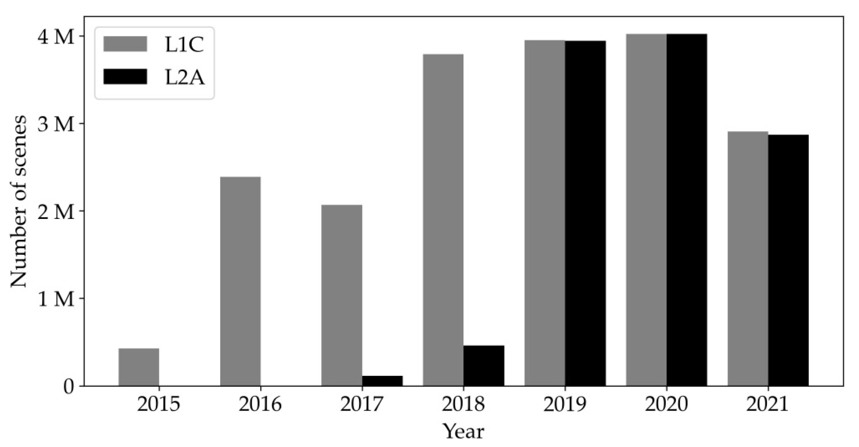
Similar to the Landsat program, the European Space Agency (ESA) has developed the Sentinel-2 mission (S2) for Earth observation, which is part of the Copernicus program [48]. It consists of a constellation with two satellites—Sentinel-2A and Sentinel-2B—each with a revisit period of 10 days, or 5 days by combining both satellites; the first satellite was launched in June 2015, and the second in March 2017. Each scene covers 110 × 110 km2, in accordance with the Military Grid Reference System (MGRS) [49]. Bands acquired by the MultiSpectral Instrument (MSI) have different spatial resolutions ranging from 10 to 20 and 60 m; the main bands of the algorithm (NIR and two SWIRs) are at 20 m, although there is also a second NIR band at 10 m. Both Level-1C (L1C) and Level-2A (L2A) products are available in GEE; L1C contains Top-of-Atmosphere reflectance, while L2A has Bottom-of-Atmosphere reflectance after the atmospheric correction is applied. A Scene Classification (SCL) is also generated in the L2A product, which labels the presence of clouds, cloud shadows, water and snow on the scene [50]. Unfortunately, the L2A product is not consistently processed for the complete S2 temporal series, and while all L1C scenes from 2019 up to the present have been processed to obtain L2A scenes, there are only a few L2A scenes available for 2017 and 2018, and none at all for 2015 and 2016 (Figure 1). Therefore, the algorithm uses either L1C or L2A scenes depending on L2A availability. Their IDs in GEE are ‘COPERNICUS/S2’ and ‘COPERNICUS/S2_SR’, respectively.
Three bands are required for BA detection in total, namely the Near Infrared (NIR) and two Short Wavelength Infrared (SWIR) bands, all of which are commonly used for BA detection [6,7,12,16,18,22,51]. Another band on the visible blue color and the quality band are used to mask clouds, and the visible red color band to reduce confusions with croplands. The exact width and location of these bands in the spectrum may vary slightly depending on the sensor, but they cover a similar spectral region (Table 1). For S2 data, the B8A and B8 bands have 20 and 10 m of spatial resolution, respectively, and are selected depending on the resolution at which BA are detected. Similarly, selection of the quality band depends on the product employed; for L2A scenes the SCL is used, and QA60 for L1C.
The BA algorithm relies on hotspots, for which there is only one product in GEE: MCD14DL, consisting of MODIS Collection 6 Near-Real-Time active fires, at 1000 m of spatial resolution [52]. The product is already rasterized by defining a 1-km-wide bounding box around the hotspot, and a confidence level from 0 to 100% is provided. The dataset is presented as a daily product, and so the detection date is known for each hotspot, but not the exact burning time. The dataset’s ID in GEE is ‘FIRMS’.
Finally, two additional products are used to identify different land covers (LC). On the one hand, the International Geosphere-Biosphere Program (IGBP) classification in the MCD12Q1 product [53], derived from MODIS data at 500 m, was used to reduce confusions at croplands and urban areas. The Copernicus Land-Cover map [54] developed at a higher spatial resolution (100 m) is also available in GEE but only for the period between 2015 and 2019, and MODIS LC map was preferred due to its longer covered period (from 2001 to 2019). On the other hand, the Global Surface Water (GSW) mask at 30 m obtained from Landsat data [55] is used to mask water bodies. This water mask contains an ‘occurrence’ band, which indicates the frequency of water presence in each pixel between 1984 and 2019, with values from 0 to 100%. The respective GEE IDs of these two datasets are ‘MODIS/006/MCD12Q1’ and ‘JRC/GSW1_2/GlobalSurfaceWater’.
2.2. Algorithm
The algorithm may be run separately on both S2 and Landsat data. The former have better spatial and temporal resolutions and thus are more accurate for BA detection, although Landsat data cover a much longer period, since the corresponding satellites have been operable since the mid-1970s. However, this algorithm is not operable for data before November 2000, as it relies on MODIS hotspots that are only available from that date onwards. The BA algorithm proposed creates one monthly BA map at a time, and so it should be run 12 times to cover the whole year. The area processed by the algorithm is bounded by a tile of the Military Grid Reference System (MGRS), irrespective of whether BA derive from S2 data (already delivered in the MGRS grid) or from Landsat images (in the WRS). BA can be detected at 10 or 20 m of spatial resolution with S2 data, or at 30 m with Landsat data.
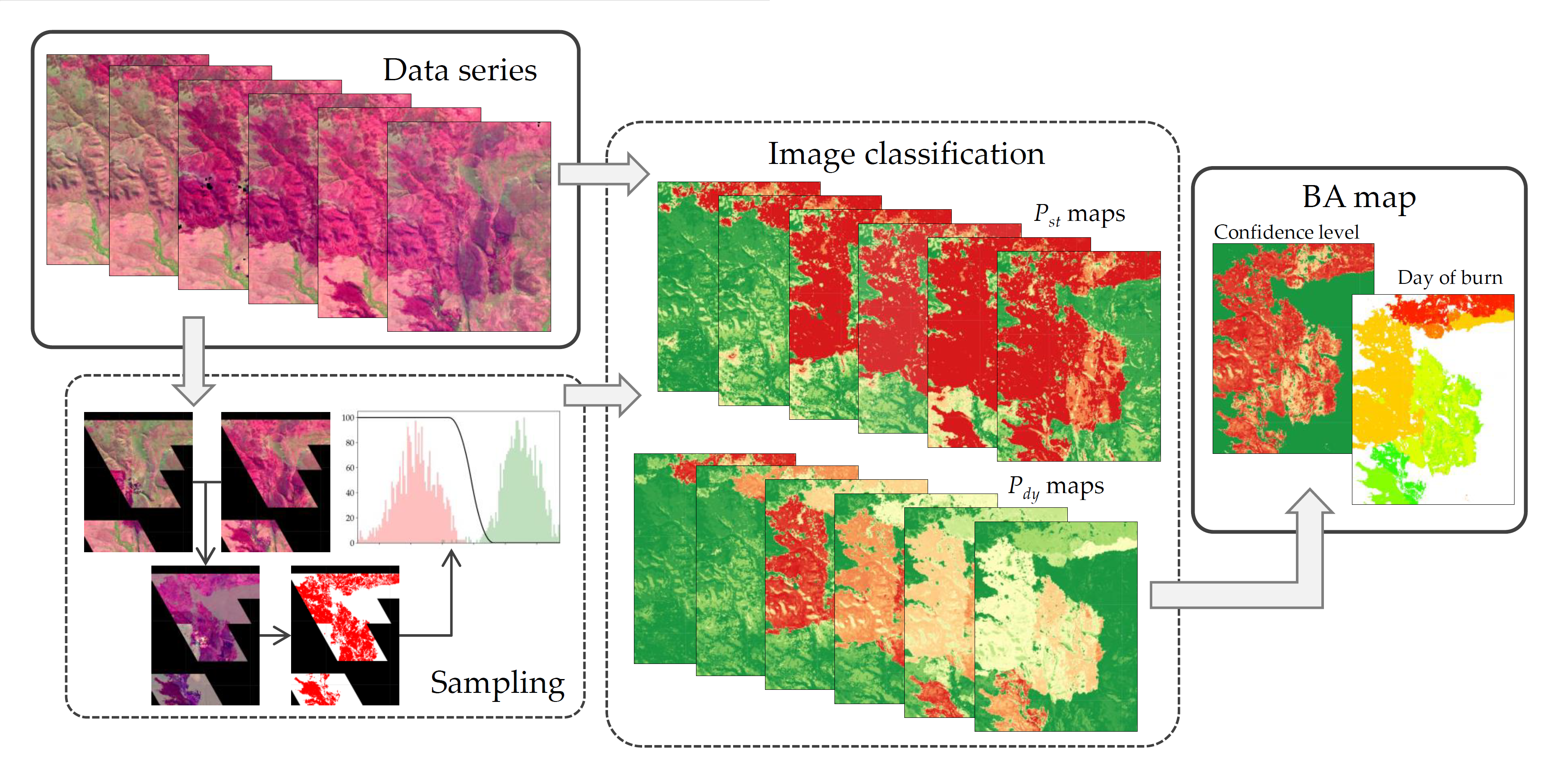
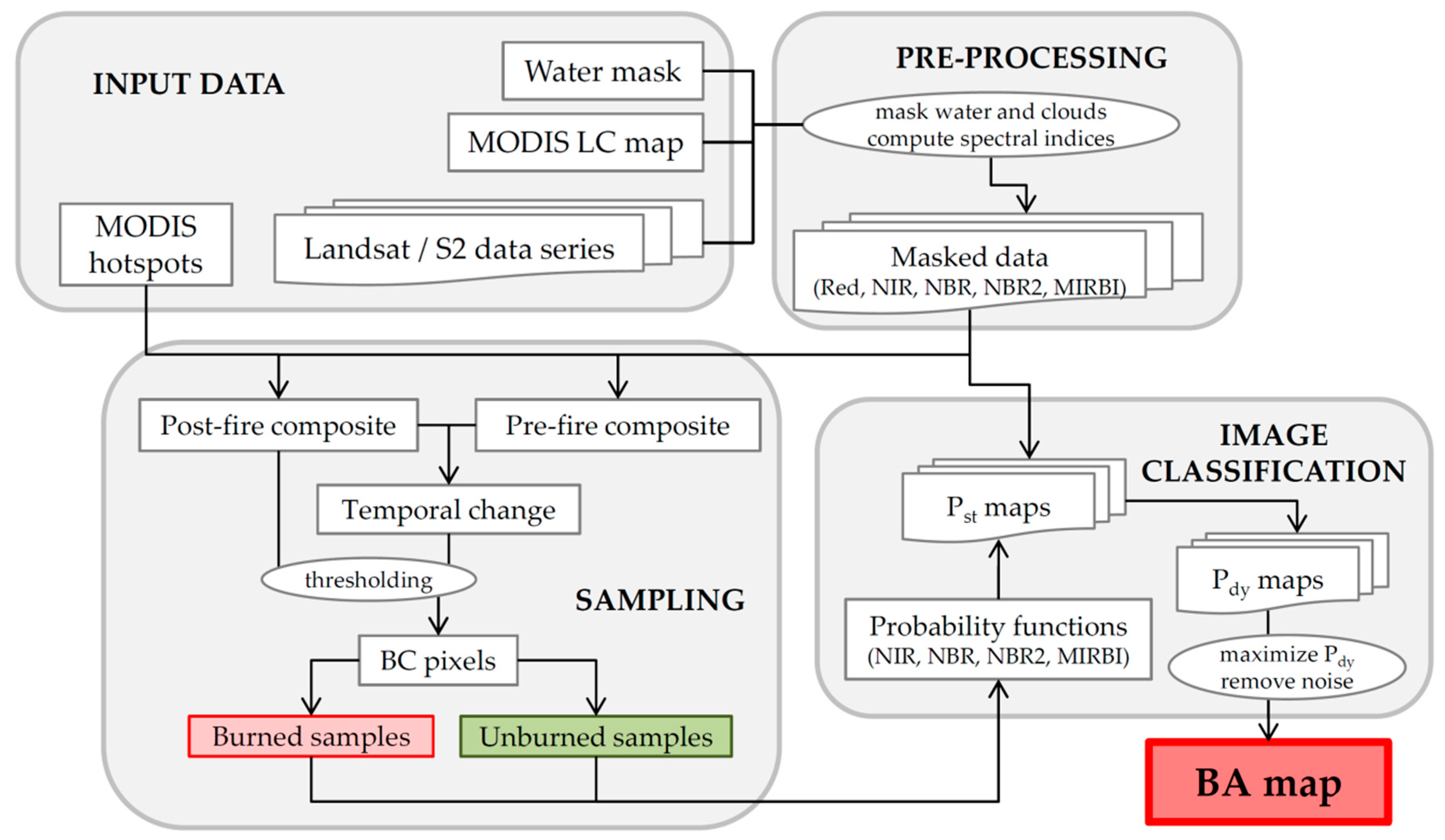
The flowchart of the BA algorithm is shown in Figure 2. It relies on one reflectance band, the Near Infrared (NIR), and three spectral indices, NBR, NBR2, and MIRBI, covering the most significant spectral areas in BA mapping; the Blue, Red and Long SWIR reflectance bands are also used to remove clouds, croplands, and cloud shadows, respectively. For every month, the spectral changes around hotspots are analyzed to identify burned candidate pixels (BC), from which burned and unburned samples are extracted. Locally adapted probability functions are defined based on those samples, and images from the data series are then classified, with each pixel being assigned a static burned probability value (Pst); depending on the temporal evolution of Pst for each pixel, a dynamic probability (Pdy) is computed. The final BA map is obtained by retaining the pixels with the maximum dynamic probability and segmenting the result to remove noise and reduce commissions. Since the algorithm is implemented in GEE, its design is restricted by the platform’s memory and processing limitations.
2.2.1. Pre-Processing
The first step involved with the BA algorithm prepares the data for BA detection, mainly by obtaining the required images, reducing the amount of data, masking clouds, cloud shadows and water bodies, and computing spectral indices.
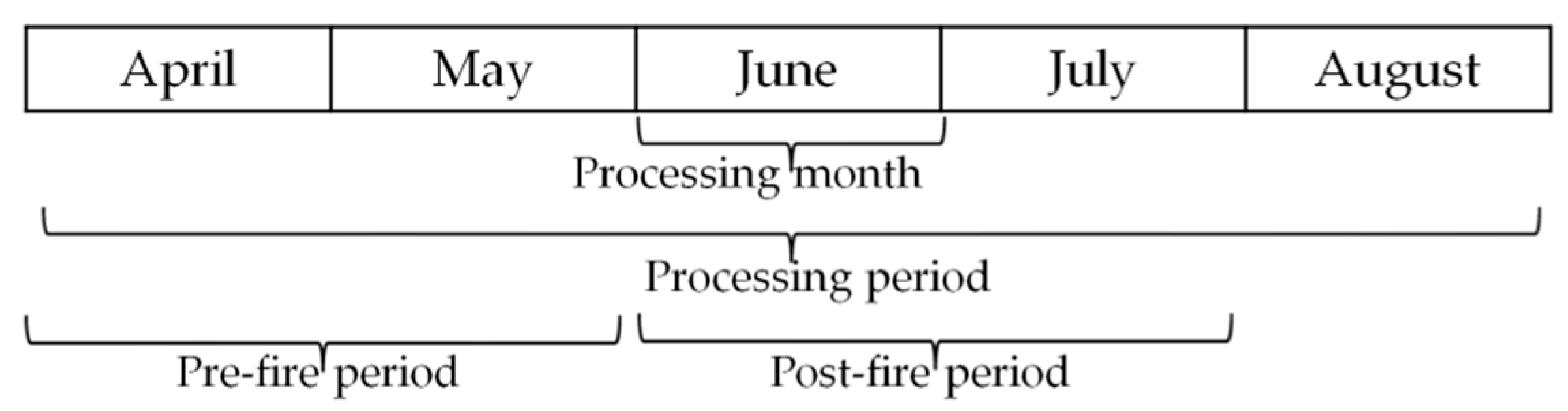
The algorithm creates a monthly map located in one MGRS tile at a time. For every month (henceforth referred to as ‘processing month’), images from 5 consecutive months are selected (called ‘processing period’), including two previous ones and a further two subsequent months (Figure 3). S2 data are already delivered in the MGRS grid, and so S2 scenes are simply selected by metadata filtering. However, Landsat data are originally in the WRS, and must be filtered and clipped by the extent of the MGRS tile, and the scenes acquired on the same day are then merged. Processing BA from Landsat data using the native WRS scenes was previously considered, but combining images from adjacent orbit swaths in overlapping areas was not plausible and prevented the full potential of the data catalog from being exploited properly; moreover, at high latitudes, this meant that every region would be processed several times—once per each orbit swath covering the region, which would prolong the process considerably. The selection of L1C or L2A scenes for S2 data depends on L2A availability in GEE, as mentioned previously. When both options are available, L2A scenes are preferred and used by the algorithm, but if the number of available L2A images is less than 90% of the number of L1C scenes in the same area and period, then L1C scenes are used instead.
A 5-month-long processing period in a MGRS tile near the Equator may contain 30 S2 scenes, with one image every 5 days (if both S2A and S2B satellites were already operable at the time), or 60 scenes if the tile is in the overlapping area between two orbit swaths. Similarly, an MGRS tile at the Equator may contain Landsat scenes from up to 38 different dates if located between two orbit swaths and with two operable satellites (Landsat-5 and 7 between 2000 and 2012, or Landsat-7 and 8 from 2013 forwards). However, the number of scenes can increase considerably at higher latitudes, where multiple orbit swaths overlapping each other may result in one image every day or around 180 images in the 5-month-long period. Since the implementation of the algorithm in such a large data series exceeds GEE’s user memory limit, several filters are applied to reduce the amount of data while maintaining the most meaningful scenes. In each step, if the data series resulting from the previous step contains more than 50 images, the following are removed:
- Images with a cloud percentage over 90%
- Images with a cloud percentage over 80%
- Images with a cloud percentage over 70%
- Images with a cloud percentage over 60%
- Images with a cloud percentage over 50%
- Images from the first and last months of the original 5-month-long period
- Images from the first half of originally the second month, and from the last half of originally the fourth month
If all filters need to be applied, 1.5 months will have been removed from the beginning and end of the original processing period, and the data series will only be 2 months long.
Once the number of images is reduced, undesired artifacts are then masked. The quality bands are used to mask clouds and cloud shadows, which are indicated in the 3rd and 5th bits in Landsat images, and in the 10th and 11th bits in L1C scenes of S2 images; since the SCL image in S2 L2A scenes have several categories, 7 different values are masked in total (Table 2). Residual clouds and snow not represented in the quality bands are masked in all three datasets by applying an empirical threshold of 0.2 in the visible blue band, where both burned and unburned areas have lower values than clouds and snow. Water bodies are not represented in the S2 L1C quality band, and so a mask obtained from the GSW product is used for both S2 and Landsat data. A conservative threshold is chosen here, masking every pixel with a frequency over 10% in the ‘occurrence’ band.
Finally, three spectral indices are computed for every image in the series: the Normalized Burn Ratio or NBR [56], the Normalized Burn Ratio 2 or NBR2 [57], and the Mid-Infrared Burned Index or MIRBI [58]. Their formulas are listed below:
where ρNIR, ρShortSWIR and ρLongSWIR refer to reflectance in the NIR, Short SWIR, and Long SWIR bands, respectively.
NBR = (ρNIR − ρLongSWIR)/(ρNIR + ρLongSWIR),
NBR2 = (ρShortSWIR − ρLongSWIR)/(ρShortSWIR + ρLongSWIR),
MIRBI = 10 ρLongSWIR − 9.8 ρShortSWIR + 2
Henceforth, the algorithm is mainly based on the NIR band and the NBR, NBR2, and MIRBI indices. The importance of these bands and indices in discriminating BA has already been analyzed and observed [18,22,59,60,61], and they ensure coverage of three different areas of the spectrum commonly used for BA detection (NIR, Short SWIR and Long SWIR) [11,13,16,18,26,27,29,31]. The NIR band selected for S2 data depends on the spatial resolution at which BA are to be detected: B8A at 20 m, and B8 at 10 m.
2.2.2. Sampling
After the algorithm’s pre-processing step, burned candidate pixels (BC) between two dates are detected based on spectral changes around hotspots, and samples for burned and unburned categories are extracted from these burned pixels, which correspond to the values observed before and after the burning of the pixel; these samples will later be used to classify images and detect BA. This identification of BC pixels is loosely based on the way burned seed pixels were identified in another study conducted for BA detection in Italy [29].
Before selecting BC pixels, clouds and cloud shadows that may have remained after the pre-processing step are further masked with two conservative thresholds, removing pixels with the following reflectance: Blue > 0.15 OR LongSWIR < 0.05. Pixels belonging to urban areas in the LC map obtained from MODIS data are likewise masked. This further masking is only applied in this sampling step of the algorithm, but not in the classification step described in the next section. Hotspots from the MCD14DL product at 1000 m, obtained from MODIS data, are filtered according to their confidence level, with those with a value lower than 80% being removed.
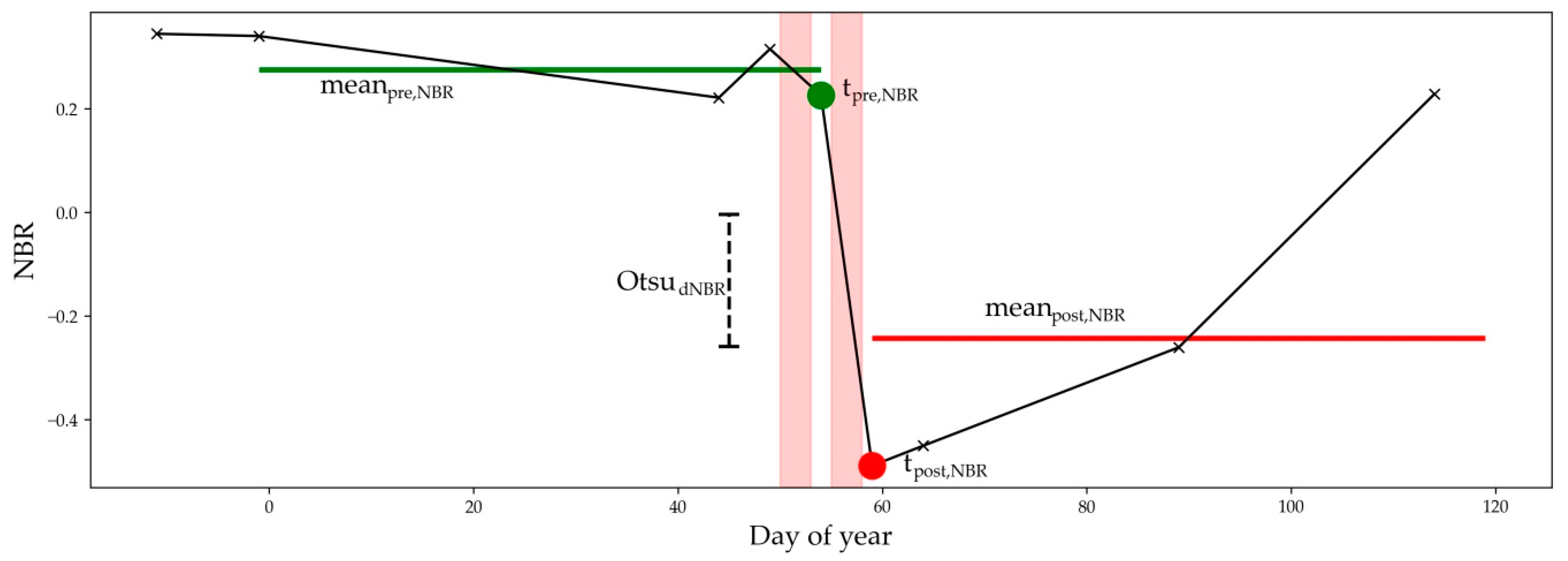
The possibility of being burned is considered for every pixel in the MGRS tile by comparing the temporal evolution of the NBR spectral index and the location and timing of active fires. For every pixel and by analyzing every pair of consecutive images in the processing month, if the pixel is covered by a hotspot between two consecutive dates, it is considered to have burned between these dates; if hotspots are found between several pairs of images, the one with the largest drop in NBR values is chosen (Figure 4). The dates between which the pixel is considered to have burned are labeled as tpre and tpost.
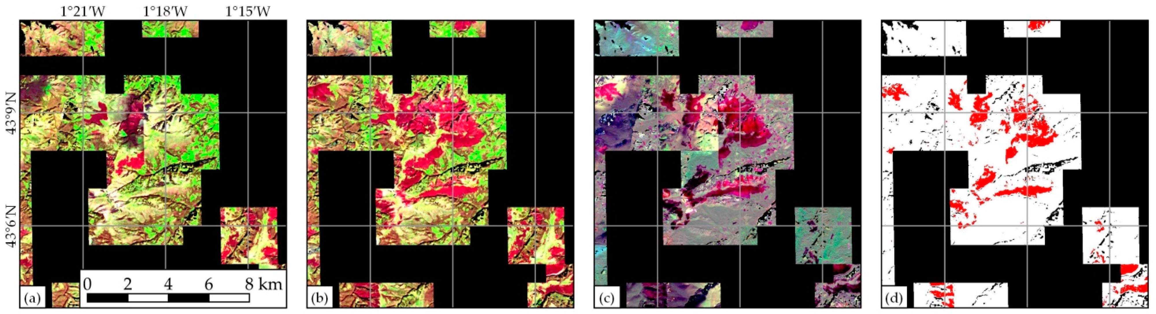
As a result, two acquisition dates with an active fire in between are obtained for every pixel in the MGRS tile (tpre and tpost), except for those where no MODIS hotspot was found. Two composite images are formed with values for every pixel from the corresponding pre- and post-fire dates (Figure 5a,b). A third temporal change image is created by a simple subtraction between tpost and tpre composites (dt, Figure 5c).
BC pixels, from which burned and unburned samples will later be extracted, are detected by analyzing the spectral signal in the tpost composite and temporal change between composites. Three groups of bands must be defined for such purpose, from which candidate pixels will later be identified. These groups of bands are:
- Temporal change of NBR, NBR2, and MIRBI spectral indices and NIR reflectance: dNBR, dNBR2, dMIRBI, and dNIR
- NBR, NBR2, and MIRBI spectral indices at tpost
- Red reflectance at tpost
The first group of bands corresponds to temporal changes. First, the Otsu threshold is computed (Otsui) for each band i, this threshold being the optimum value that separates the image in two classes by minimizing the inter-class variance, considering that pixels have a bimodal distribution [62]. At the same time, two additional values are computed for each pixel: the mean value of the band over the two months prior to the pre-fire date (meanpre,i), and the mean value over two months following the post-fire date (meanpost,i) (Figure 4). In any band i (NBR, NBR2, MIRBI and NIR), pixels are labeled as BC pixels in that band if they meet two conditions, as shown in this formula for band NIR:
BCdNIR = (dNIR < OtsuNIR) AND (meanpost,NIR − meanpre,NIR < OtsuNIR/2),
The temporal change being larger than the Otsu threshold ensures that there was some significant spectral change in the BC pixel that might be caused by a fire. Meanwhile, the difference between mean values from both periods also denotes that this change was prolonged over time, even though this requirement is not so strict (only half the Otsu threshold), because the vegetation may recover during the post-fire period (Figure 4). Please note that the conditions above are suitable for spectral indices and reflectance that decrease when burned (NBR, NBR2 and NIR), while the MIRBI index increases its values in burned areas, and so opposite signs should be used in such case. Additionally, the presence of hotspots does not necessarily mean the presence of burned areas, and so some empirically obtained minimum values for Otsu thresholds are required to reject false detections: −0.05, −0.05, 0.25 and −0.02 for dNBR, dNBR2, dMIRBI, and dNIR bands, respectively. If the threshold computed initially in any band is closer to 0 than this minimum, then it is replaced by this value.
The second group of bands is based on post-fire values (NBR, NBR2, and MIRBI at tpost). The Otsu threshold is also computed for each band among the pixels in the composite. The BC pixels in each band (BCpost,NBR, BCpost,NBR2 and BCpost,MIRBI) are simply those with a value lower than the threshold (higher in the case of MIRBI). This makes sure that BC pixels, in addition to the drop observed in the first group of bands, evidence the strongest burned signals in the image, since some events unrelated to fires (such as deforestation and floods) could exhibit a sudden decrease similar to burned areas even if they did not show such a strong-burned signal on the post-fire date. The NIR reflectance band was not included in this case, because its post-fire reflectance was found to be too variable in some biomes.
Finally, the third group is based on only one band: tpost reflectance in the visible red band, with pixels with a reflectance below Otsu threshold being labeled as burned candidates (BCpost,Red). This band was primarily included because according to literature on the subject it is the best band to discriminate between burned areas and agricultural false positives [60], since croplands are a well-known source of commission errors in BA mapping due to their spectral similarity to burned areas [18,22,26,27].
Final BC pixels are selected by combining BC pixels from the three previous groups of bands:
- In the first group of bands, pixels must be labeled as BC in at least 3 out of 4 bands (BCdNBR, BCdNBR2, BCdMIRBI, and BCdNIR)
- In the second group, they must be labeled as BC in at least 2 out of 3 bands (BCpost,NBR, BCpost,NBR2 and BCpost,MIRBI)
- In the third group, being labeled as BC in the Red reflectance band at tpost (BCpost,Red) is mandatory
The result is a group of pixels with a strong-burned signal, located both spatially and temporally around a MODIS hotspot (Figure 5d).
Even though the criterion for the red reflectance band at tpost removes many false positives from croplands, further restrictions are applied in the first group of bands. For pixels identified as crops in the IGBP classification of the MCD12Q1 product at 500 m, the thresholds used in both conditions are multiplied by 2:
BCdNIRcrops = (dNIR < 2·OtsudNIR) AND (meanpost,NIR − meanpre,NIR < OtsudNIR),
The criteria for detecting BC pixels are quite strict to avoid commissions, and selected pixels represent burned areas with a high severity, frequently omitting pixels with a lower severity. Next, 1000 samples are extracted in total from the BC pixels. The unburned category is composed by NIR, NBR, NBR2, and MIRBI values of BC pixels in the pre-fire composite (tpre), while the same values in the post-fire composite (tpost) form the burned category. Thus, all samples are in the same pixels, although unburned values were observed before the BC pixels were burned, with burned values being observed after the burning. These unburned and burned samples will then be used as training samples for image classification.
Finally, to avoid false detections as a consequence of hotspots not pointing to actual burned areas, two criteria must be met along the sampling step of the algorithm:
- Hotspots filtered temporally between composites’ dates must cover a minimum surface of 5 km2 in the whole MGRS tile
- Burned candidate pixels must cover a minimum surface of 1 km2
If either criterion fails, the algorithm assumes that no area was burned in the region or that the available data are insufficient for the purpose of detecting any BA. In such case, the algorithm skips the following image classification step and returns an output image with no BA.
2.2.3. Image Classification
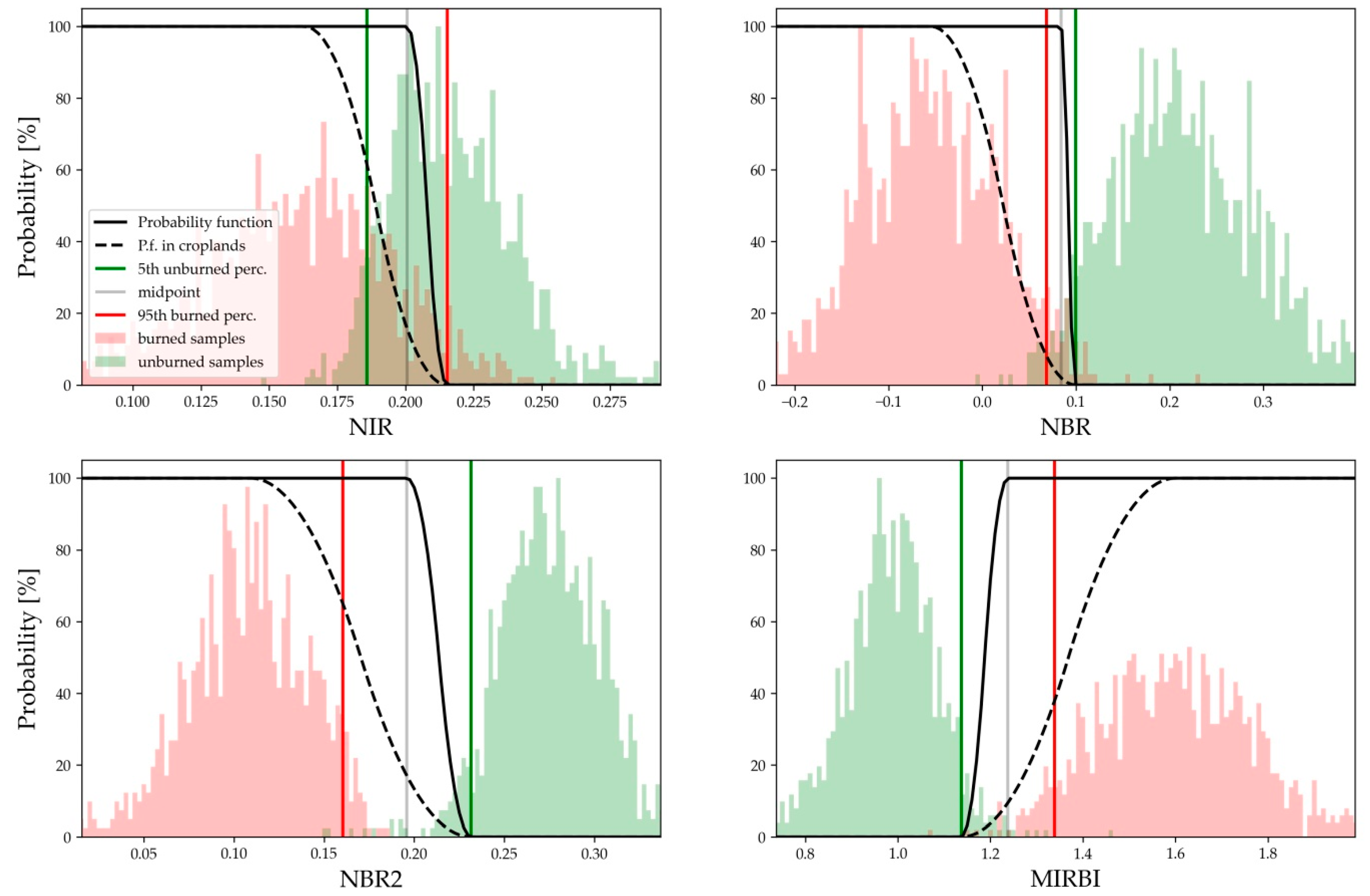
Samples extracted in the previous section are employed to classify the individual scenes from the pre-processed series. The strict masking used at the beginning of the sampling step is not applied here; the data series resulting from the pre-processing is used instead. For each band (NIR, NBR, NBR2, and MIRBI), a probability function is defined based on a logistic function, which is a smooth transition between two classes, this having already been used for BA detection in several studies [18,63,64,65,66]. The function is s-shaped for the MIRBI index, but z-shaped for the rest of the bands (Figure 6). To define the boundaries of the logistic curve, the 95th percentile of the burned samples and the 5th percentile of the unburned samples are computed, with the objective being to adjust the logistic curve between these two percentiles. However, the strict criteria for BC pixel detection may have omitted pixels with lowest burn severity, and so the logistic curve is shifted closer to the unburned distribution. Therefore, a midpoint between both percentiles, located halfway between both values, and the 5th unburned percentile are used as boundaries of the curve, which correspond to 100% and 0% of probability values, respectively. If the distributions of both categories overlap each other, the 95th burned percentile may be higher than the 5th unburned percentile; in this case, the logistic curve is adjusted between the midpoint and the 95th burned percentile (NIR in Figure 6). Additionally, note the reverse order of all parameters for the MIRBI spectral index. BA detection in croplands is more restricted than in other LC categories: the upper boundary of the logistic curve, corresponding to a 100% probability, is placed at the 50th percentile or median of the burned distribution.
Along with the probability function, the discriminability of burned areas is also measured for each band. This is computed using the M separability index (Equation (4)) [67], which has been employed in several studies for BA detection [18,30,68,69,70].
where μb and μub are the mean values of burned and unburned samples, respectively, and σb and σub the standard deviations of the same categories.
M = |μb − μub|/(σb + σub),
The four probability functions are applied on every image of the data series, each on the corresponding band, which results in four probability images for every date in the series (Figure 7a–d), with values ranging from 0% (unburned) to 100% (burned). These are aggregated into one probability image by computing a weighted average, with the weight being equal to the square of the separability index, using the following formula:
where Pi and Mi are the probability and the separability index of the band i (NIR, NBR, NBR2, or MIRBI). This Pst value, referred to as static probability, indicates the probability of being burned on that date (Figure 7e), regardless of whether the pixel was already burned on a previous date in the series.
Pst = ∑ Pi Mi2/∑ Mi2,
Once every image in the data series has been assigned the static probability (Pst), the temporal evolution of this Pst is analyzed to detect the date immediately after the pixel was burned. For this purpose, a second probability, called dynamic probability (Pdy), is computed for every pixel from every date in the data series based on three measures:
- Ppre: mean Pst during previous two months, up to the corresponding date
- Pt: Pst on the corresponding date
- Ppost: mean Pst during next two months, immediately after the corresponding date
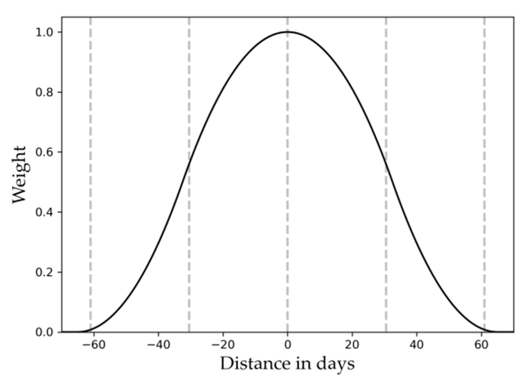
The mean probabilities from the previous and following months (Ppre and Ppost) are weighted averages, with highest weights for dates closer to the day for which Pdy is being computed. A logistic function is used to estimate these weights based on the distance from the central day; this function is adjusted to fit in the over-4-month-long period, with weights reaching the 0 value after a distance of two months (Figure 8). This weighted average enables burned pixels to be detected in biomes where the vegetation is regenerated in a few weeks, such as in tropical regions [71,72,73].
High values of Pdy should only be found when pixels are observed as having burned for the first time, which should correspond to the first available image after the actual burning date. These fires appear as sudden increases in static probabilities and are maintained high over several consecutive acquisitions: a low probability on previous dates (Ppre) and high values on the corresponding date and following ones (Pt and Ppost) are required. The following formula is used to compute this dynamic probability:
Pdy = (100% − Ppre) · Pt · Ppost,
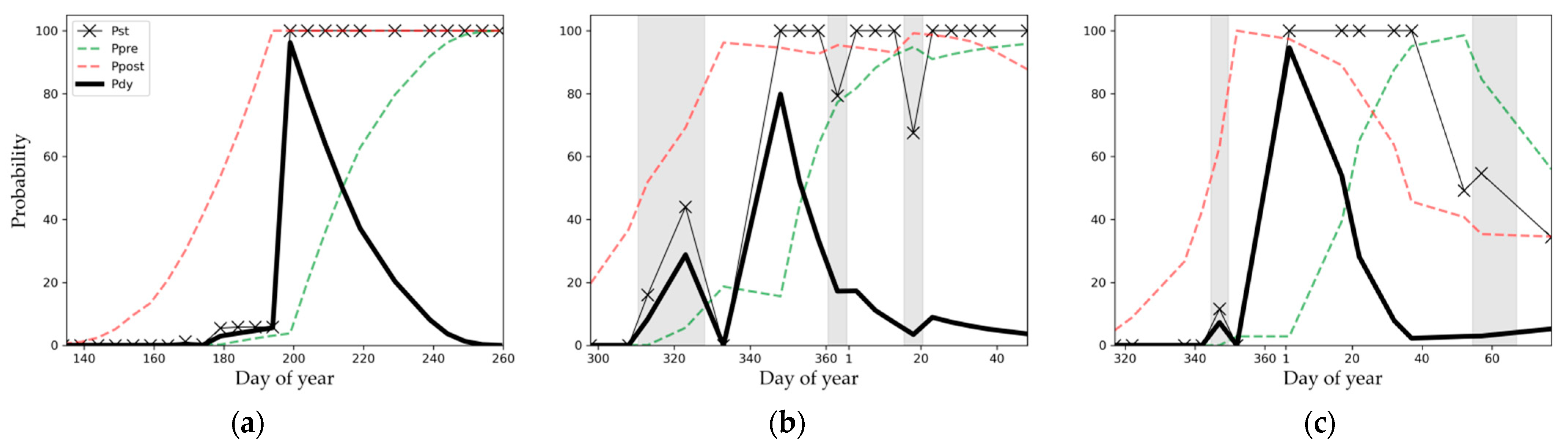
A low Pdy will be computed for pixels already burned on previous dates, since those pixels will show a high Ppre (Figure 9). Similarly, sudden increases in Pst values that decrease again in the next image, usually belonging to clouds and cloud shadows unmasked in the pre-processing step, will have a low Pdy, because the Ppost from the following dates will be low. However, clouds and shadows, despite having a low Pdy, may cause a decrease in dynamic probability on a nearby date that corresponded to an actual burning (Figure 9b).
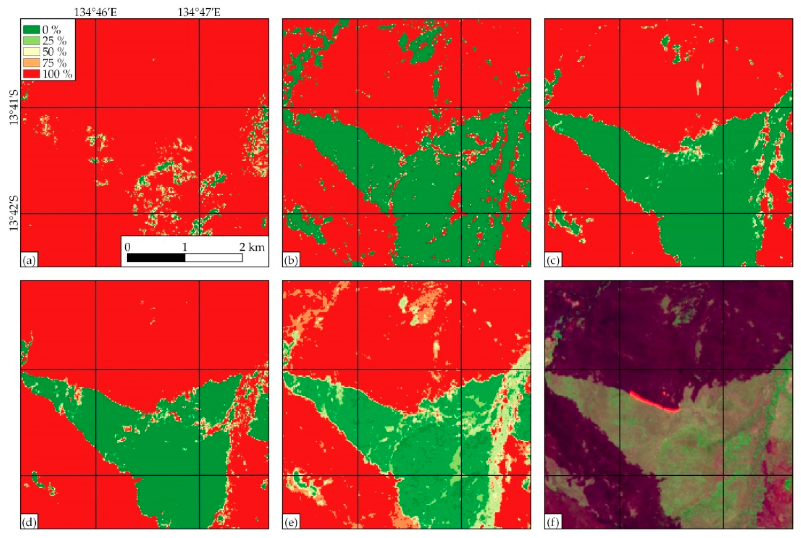
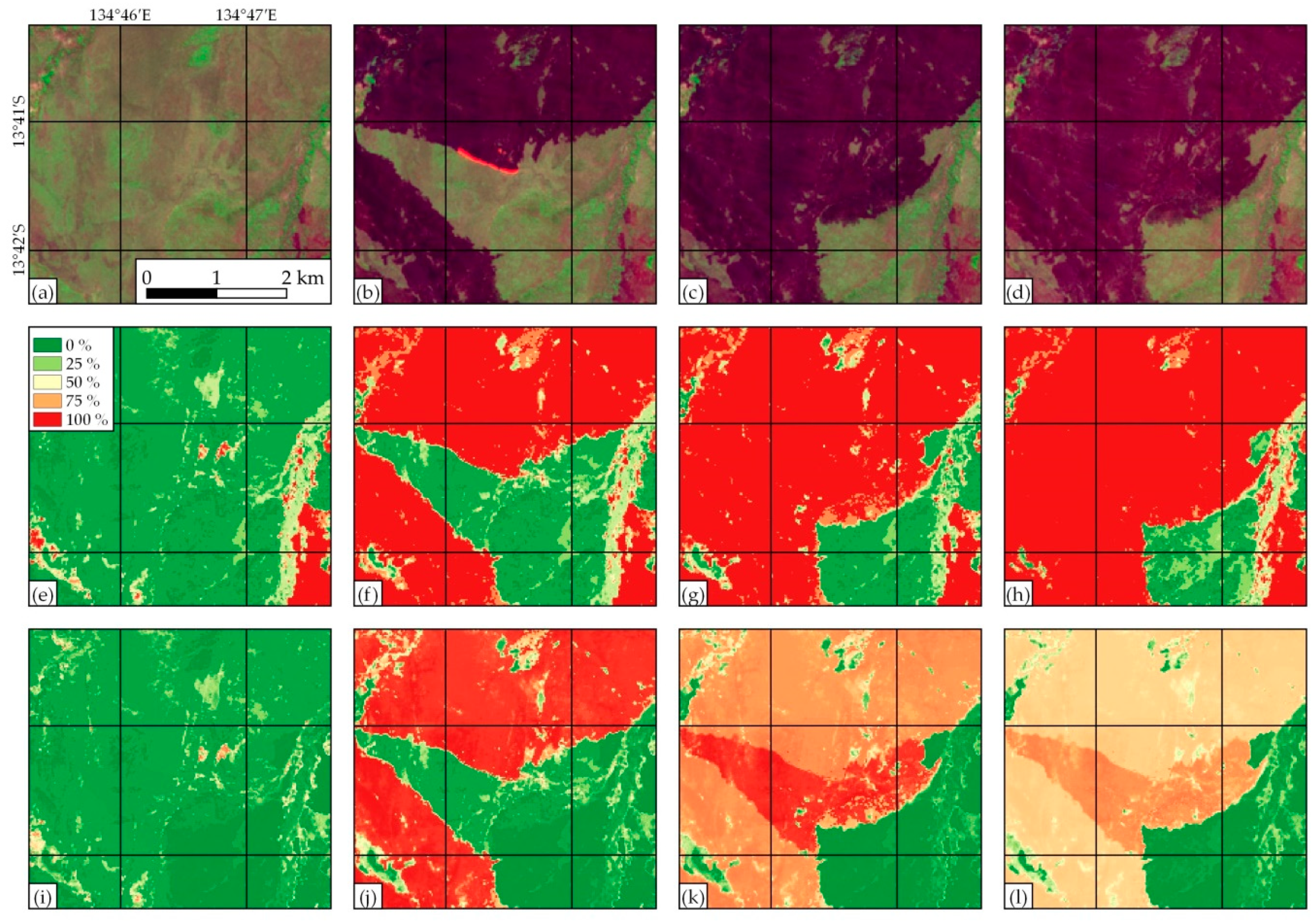
Therefore, for every image in the data series (Figure 10a–d), two series of probabilities are obtained. The Pst maps indicate the probability of being burned on each date, even if they have been already observed as burned in previous images (Figure 10e–h); meanwhile, the Pdy maps show the probability of having burned on the considered date for each pixel (Figure 10i–l), showing a high value on the first date after burning but lower probabilities on the following dates. The BA algorithm then creates a temporal composite from this Pdy map series, by selecting the date with highest dynamic probability for each pixel (Figure 11a).
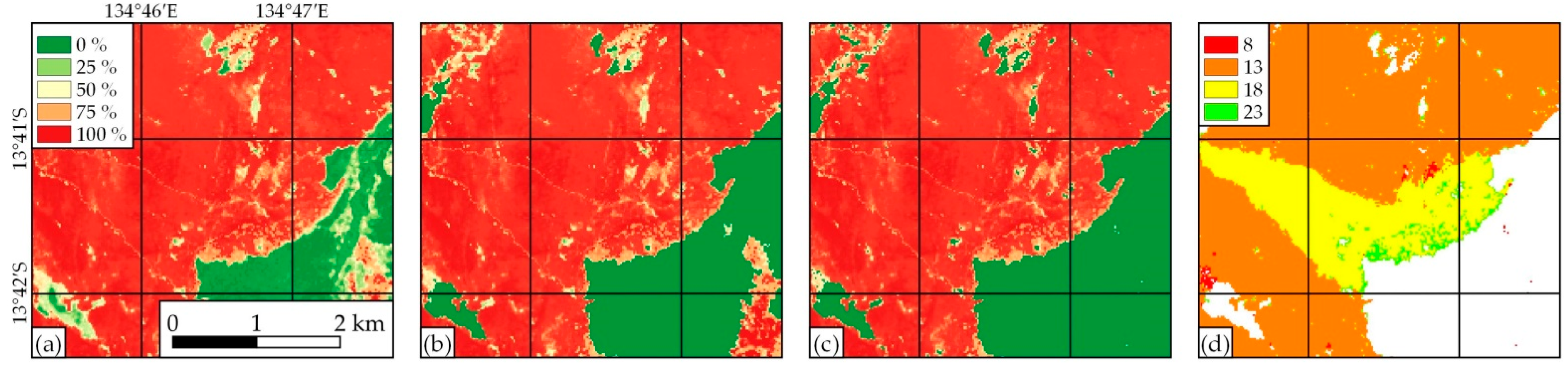
The composite with the maximum Pdy may also contain pixels with low burn probability values and some areas burned on dates outside the processing month that should be removed (Figure 11a). The best option for removing these areas would be a two-phased strategy involving first identifying burned seeds (pixels with a strong-burned signal) and then extending the burned region around these seeds up to a threshold [66]; this strategy has already been used extensively for BA detection [12,13,16,18,22,25,39,41,61]. Several approaches were tested to implement this strategy, such as spatial dilation from burned seeds, cumulative cost maps, and grouping of connected pixels, although they all proved to be too time- and memory-consuming and always ended up exceeding GEE’s user memory limit. An alternative methodology was applied instead in the form of the Simple Non-Iterative Clustering (SNIC), a non-iterative superpixel segmentation algorithm [74] already implemented in GEE that has been shown to be efficient in terms of computation and memory requirements [75]. An 8-neighbor connectivity was used with a 0 compactness (disabling the spatial distance weighting) and 10 pixels as a superpixel seed location spacing parameter [74], which was observed as being a balanced value between the size of the objects and well limited burned patches. Once the object images are obtained, the mean value of each object is then computed in GEE. Only the objects with a mean Pdy higher than 50% are labeled as burned. The segmentation also removes single pixels with probabilities higher than 50% that are part of clusters with low BA probabilities, which would otherwise lead to commission errors (Figure 11b).
Finally, every pixel whose highest Pdy in the processing period was not observed in the processing month is labeled as unburned, and pixels that could not be observed on a single day throughout the processing month are assigned a special value of −1. The resulting BA map contains two bands (Table 3): the Pdy value as a confidence level of the burned pixel (Figure 11c), and the date of burn, which corresponds to the day of the year on which the highest Pdy was observed (Figure 11d). The final BA map is exported to a GeoTIFF image covering the corresponding MGRS tile in UTM coordinates, at 10, 20 (when using Sentinel 2 data) or 30 m (when using Landsat data) of spatial resolution.
2.3. Quality Assurance
2.3.1. Reference Data
The Committee on Earth Observing Satellites’ Land Product Validation Subgroup (CEOS-LPVS) defined validation as the process of assessing by independent means the accuracy of the data products from the system outputs [76]. Out of four validation stages defined by CEOS-LPVS, Stage 3 requirements are usually followed by BA product validations [16,18,20,21,41,77,78], which consist of an assessment characterized in a statistically robust way over multiple locations [79]. BA products are validated by comparison with reference data (RD) created in multiple image pairs and located in validation sites typically selected by stratified random sampling [20,77,80,81]. These RD are generated by visual analysis and supervised classification from independent higher-spatial-resolution images [82].
Validation of medium-spatial-resolution products in accordance with the CEOS protocol is challenging as the availability of multi-date higher-spatial-resolution data is expensive and often unavailable [31]. Although a standard BA reference database is already available for the scientific community, these data do not include information from 2016 onwards (the years in which sufficient S2 data can be found) or are limited to a country or continent (CONUS and Africa) [83], and could not be used to assess our algorithm’s performance globally on S2 data. In this study, a quantitative assessment of our algorithm was carried out by comparing it with BA interpreted visually from multi-date S2 data at 10 m at 50 sites. This is a low number of sites if compared with other studies, where around 100 [77] or over 500 [21] validation areas were used, even though those sites were composed by only two images. A subset of 20 × 20 km2 was selected for each site instead of a complete scene (110 × 110 km2) to obtain an accurate result by supervised classification without requiring manual refinement. Similar sizes have already been used in other studies, especially when this has concerned Landsat data with SLC-off problems [18,77,84]. Unfortunately, both the RD and the results of the BA algorithm at 10 and 20 m were obtained from the same data—S2 imagery—because generating a similar global sample from higher-resolution data was unfeasible. Moreover, the stratified random sampling for site selection was based on S2 data, which means that all sites have frequent available cloud-free S2 images, making them optimum sites for BA detection using data from the same source. Therefore, due to the small size and low number of sites, same data being used for both the RD and the algorithm, and the site selection favoring S2 cloud-free areas, the authors prefer to use the term ‘quality assurance’ (QA) for this exercise, rather than a validation.
The areas where the QA analysis was carried out were selected using the stratified random sampling methodology [81], based on S2 data, with sampling units being 20 × 20 km2 windows located at the center of each MGRS tile. Although a high number of areas is optimal in achieving an accurate estimation of errors in a global algorithm, processing of fewer albeit representative QA sites with temporally longer periods was preferred, which is especially crucial for assessing Landsat-based results and limiting the effect of any acquisition date disagreement. This QA exercise was limited to 50 areas—with several image pairs analyzed at each one—and is deemed to be sufficient since it covers several biomes. This sampling methodology has already been implemented in GEE as the VA tool from Burned-Area Mapping Tools (BAMT) [41] and, even though it could not be used globally because it exceeds the GEE user memory limit in large areas, part of its code was used in order to access the S2 catalog and analyze its availability in GEE. The whole analysis was carried out for data from 2019, which is the first year when S2 L2A data have already been consistently processed (Figure 1). First, long sampling units were selected, at least 2 months long, with a minimum frequency of one image every 20 days and cloud coverage lower than 20%. Then, these long sampling units were assigned the predominant Olson biome [85], reclassified into 7 main classes, and low or high fire activity in the unit’s area. Global VIIRS active fires at 375 m were used in this study [86], which were observed as better detecting small fires [87] than the BA products at coarse resolution typically used as fire activity estimations [41,80,81], which tend to underestimate small fires [16,17]. Lastly, after splitting sampling units into 14 strata according to the 7 major Olson biomes and low and high fire activities, 50 QA areas were then randomly selected from each stratum. The number of sites in each stratum was proportional to the total number of sampling units and the mean fire activity in the stratum.
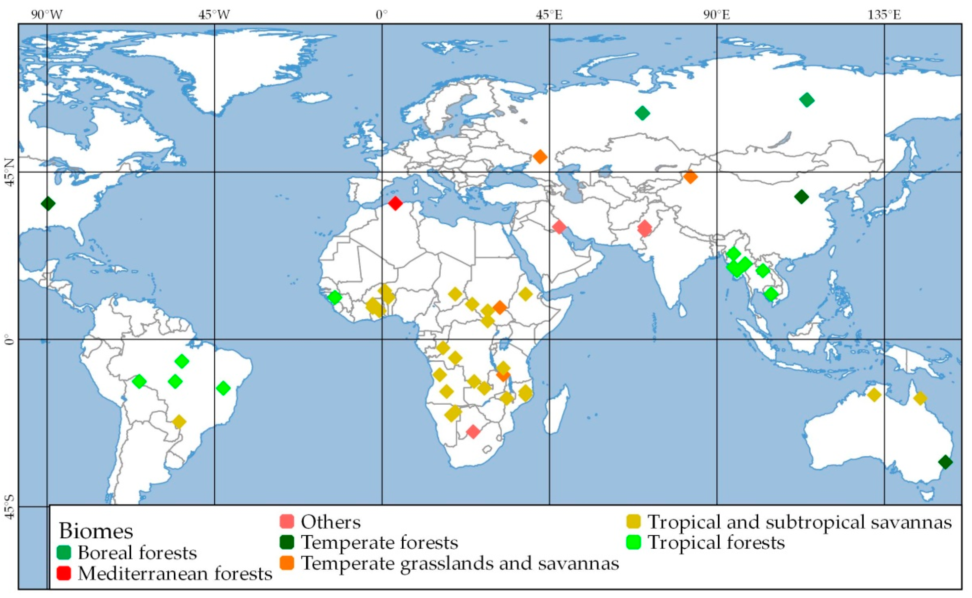
The 50 QA areas selected by the stratified random sampling can be seen in Figure 12. Despite sampling units being split among 7 major Olson biomes, half of the QA sites are in the tropical and subtropical savannas biome, because this is the biome with most African fires, constituting 70% of global BA. The following biome with most QA sites is tropical forests with 11 sites, most of them located either in Brazil or on the Indochinese Peninsula; the remaining biomes contain between 1 and 4 sites. The shortest periods are two months long, while some cover the whole year of 2019, although most are less than 8 months long. Among all 50 sites, 419 cloud-free images were used, which means 369 pairs of consecutive images. The complete list of QA areas and their main characteristics are detailed in Appendix A Table A1.
For every pair of consecutive cloud-free images in each QA area, RD were created using a supervised classification, derived from S2 data at 10 m of spatial resolution. This task was done using the RP tool for reference data creation from BAMT, implemented in GEE [41]. Exported results were visually checked by comparing them with pre- and post-fire color images in a local machine and reprocessed in GEE where necessary, but were not refined or modified manually. Reference perimeters from different pairs of images at the same QA site were merged in one final image, in which every pixel was labeled as unburned, burned, or unobserved.
2.3.2. Accuracy Metrics
The algorithm presented in this study was run on all 50 QA sites, processing every month included between the first and last dates of each site, and at three different spatial resolutions: 10 and 20 m with S2 data, and 30 m with Landsat images. These BA maps shall be referred to BAS2-10, BAS2-20, and BAL-30 from now on.
Accuracy metrics were estimated based on the error matrix approach [88,89], by comparing BA maps with RD at the QA sites. Commission and omission errors (CE and OE) and the Dice coefficient (DC) were computed for each QA area, together with an aggregation from the sum of error matrices. DC is defined as the probability for a classifier to identify a pixel as burned, given that the other classifier also identifies it as burned [81,90,91], with the BA maps obtained by the automatic algorithm and the RD being the two classifiers in this case. In addition to the accuracy metrics for BAS2-10, BAS2-20, and BAL-30, the global products FireCCI51 and MCD64A1 were also assessed at these 50 QA sites. The only global product at medium resolution, GABAM, could not be assessed because this product lacks the date of burn. The accuracy of the BA maps and global products was also analyzed in different LC categories using the IGBP classification from the MCD12Q1 product at 500 m, reclassified into 9 main classes (Table 4).
2.3.3. Reporting Accuracy
A reporting accuracy analysis was carried out for all 5 BA products in these 50 QA areas by comparing burning dates from VIIRS active fires and those from BA products, following several previous studies [12,16,18,92]. After drawing a 375 × 375 m2 window around each hotspot inside a QA site, the number of days between the hotspot and the first burned pixel detected by BA products in the window is measured, with this burned pixel being considered part of the BA whose fire was recorded by the hotspot. The purpose of this indicator is to measure the BA detection delay when labeling the date of the fire.
2.4. Test Sites
In addition to the QA exercise, performance of the proposed preliminary algorithm was tested in three large regions of 5 × 5 degrees, covering three representative biomes. The purpose of this analysis is to ensure that the algorithm is sufficiently robust to generate plausible results and assess the limitations of the medium-spatial-resolution algorithm, such as acquisition gaps owing to persistent clouds or issues related to active fires.
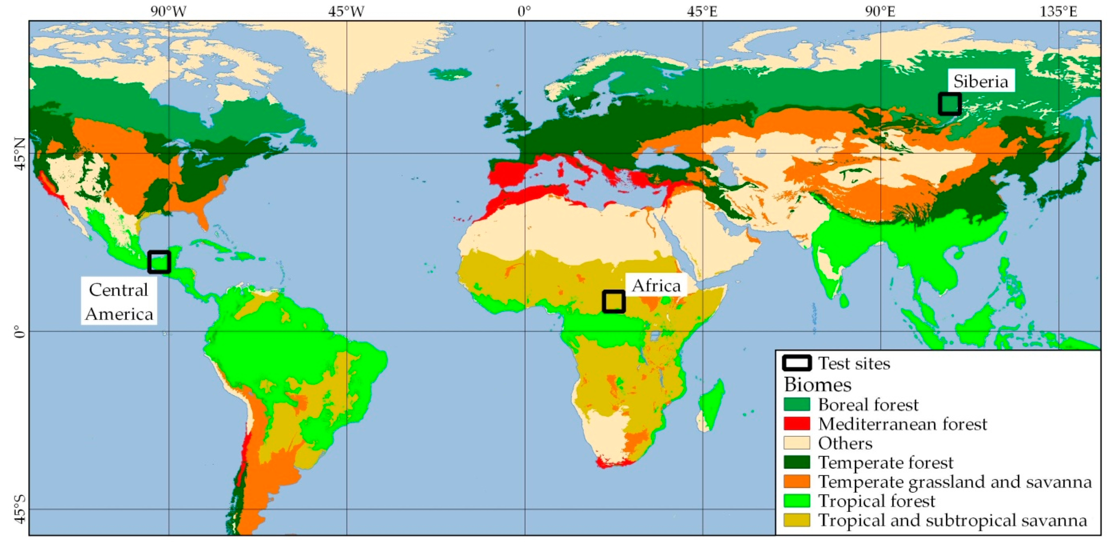
Stratified random sampling was used to select these three sites, similar to QA site selection; however, S2 image availability and cloud coverage were not taken into account in this case. Sampling units, consisting of MGRS tiles, were assigned the predominant Olson biome in the region, and the number of VIIRS hotspots detected in 2019 was used as fire activity. Once all units had been classified into 14 strata (7 major Olson biomes and low/high fire activity), the 3 strata with the highest mean fire activity were then selected. One sampling unit was randomly selected from each of these 3 strata, and 5 × 5-degree windows around these units were selected as test sites (Figure 13). The test site from Africa is located on the eastern half of the Central African Republic and contains predominantly tropical and subtropical savannas; the site from Central America is located between Mexico and Guatemala and includes tropical forests; the third one is in Siberia, north of lake Baikal, and is covered by boreal forests. The whole year of 2019 was processed at all three sites with S2 data at 20 m (BAS2-20), which was proven to be the fastest and one of the most accurate resolutions (see Section 3.1 and Section 3.2).
The results obtained at these test sites at 20 m were compared with three global BA products at different resolutions: FireCCI51 at 250 m, MCD64A1 at 500 m and GABAM at 30 m. To analyze the spatial patterns of BA, the fraction of burned surface in a 0.05 × 0.05 degree grid (≈5.5 × 5.5 km2 at the Equator) was compared between BAS2-20 and each global product.
3. Results
3.1. Algorithm
The algorithm presented in this study was run in the 50 QA areas at three different spatial resolutions (S2 at 10 and 20 m and Landsat at 30 m), with 321 monthly BA maps in total created at each resolution. Processing times depended on the resolution selected, with 20 m (BAS2-20) being fastest, which took 4.2 min per monthly map on average, followed by 30 m (BAL-30) at 4.5 min/map, and with the 10 m resolution (BAS2-10) being the slowest at 5.9 min per BA map.
3.2. Accuracy Metrics
Accuracy measures obtained by comparing the RD with our BA maps and global products are shown in Table 5. Commissions, initially between 18–19% for global products at coarse resolution (MCD64A1 at 500 m and FireCCI51 at 250 m), decreased up to 11% for BA maps derived from Landsat data (BAL-30), and around 9% at both resolutions with S2 images (BAS2-20 and BAS2-10). Similarly, omissions decreased from over 50% to less than 35% for BAL-30 maps, and between 27–28% for maps obtained from S2 data. Dice coefficients followed the same trend, since lowest values were found for products at coarser resolutions (56–62%), followed by 75% for BA maps at 30 m and over 80% at 20 and 10 m. Accuracy metrics at specific QA sites area are shown in Appendix A Table A2. No major improvement was found when processing S2 data at 10 m over 20 m, even though both commissions and omissions decreased slightly. Around 4300 and 4000 km2 of burned areas were detected at these 50 sites by our algorithm using S2 and Landsat data, but significantly less by products at coarse resolution: 3355 and 2824 km2 by FireCCI51 and MCD64A1, respectively. According to RD, however, 5421 km2 had actually burned.
Figure 14 shows the accuracy measures in different LC categories. More than half the burned area in these 50 QA areas (56.9%) was in savannas, where our algorithm performed best with commissions between 8–9%, omissions between 18–27%, and Dice coefficients between 81–86%, depending on the spatial resolution. Next were grasslands, with 19.3% of total BA and slightly lower omissions but higher commissions, followed by croplands and forests (12.7 and 10.9% of total BA, respectively), both with low commissions but also very high omissions (45–70%). Very few areas were burned in shrublands (0.2%) or in urban areas (0.1%), and practically none in the remaining three LC categories (snow, ice, and water bodies, wetlands, and barren). In all these land covers, commissions were lower for BA maps obtained from S2 data (BAS2-10 and BAS2-20) than for those from Landsat images (BAL-30), while omissions remained in some cases. Global BA products at coarse resolution showed significantly higher omissions in most land covers, except in croplands, and similar or higher commissions; Dice coefficients were higher as spatial resolutions improved, being similar only in croplands.
3.3. Reporting Accuracy
A total of 13,730 VIIRS hotspots were located at the 50 QA sites, detected between the corresponding first and last dates for each site. BAS2-10 maps contained some burned pixel around 87.4% of these hotspots, with lower ratios for BAS2-20 (84.5%) and BAL-30 (78.9%). Products at coarse resolution showed significantly lower detection percentages—41.0% and 35.9% for FireCCI51 and MCD64A1, respectively—which means omitting around 60% of the fires detected by VIIRS hotspots.
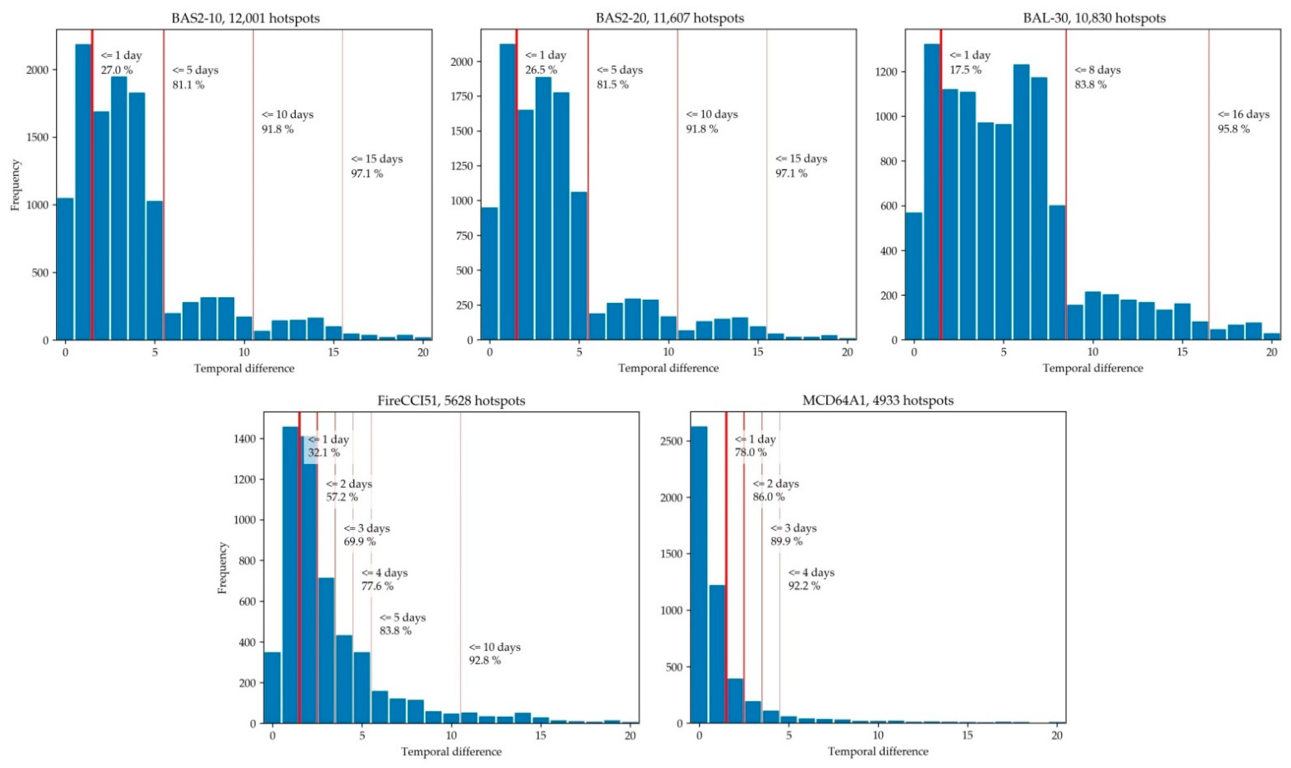
Over 26% of BA was detected the same day or the day after the hotspot’s date in BAS2-10 and BAS2-20, and 17.5% in BAL-30 (Figure 15). All three of them had detected at least 81% of BA the first 5 (for BAS2-10 and BAS2-20) or 8 days (BAL-30), which correspond to the maximum time needed for S2 and Landsat satellites to revisit the area, respectively. Likewise, by the time a satellite revisited the area for the second time after the hotspot’s date (10 and 16 days for S2 and Landsat data), BA had already been observed and detected by the algorithm for nearly 92% of the hotspots. In comparison, global BA products detect burned areas earlier, due to their better temporal resolution (1 day). In particular, MCD64A1 detected 78.0% of BA the same day or one day after the hotspot, and 86.0% after two days; FireCCI51 took longer, with only 32.1% detected the same or next day, and not exceeding 80% of detection until the 5th day.
3.4. Test Sites
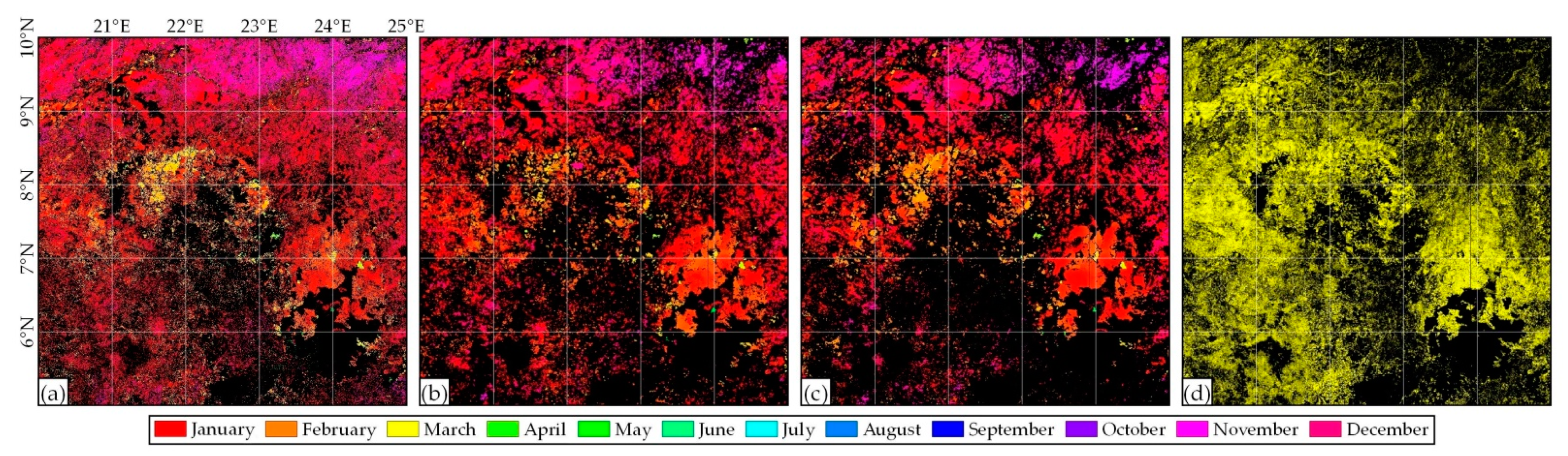
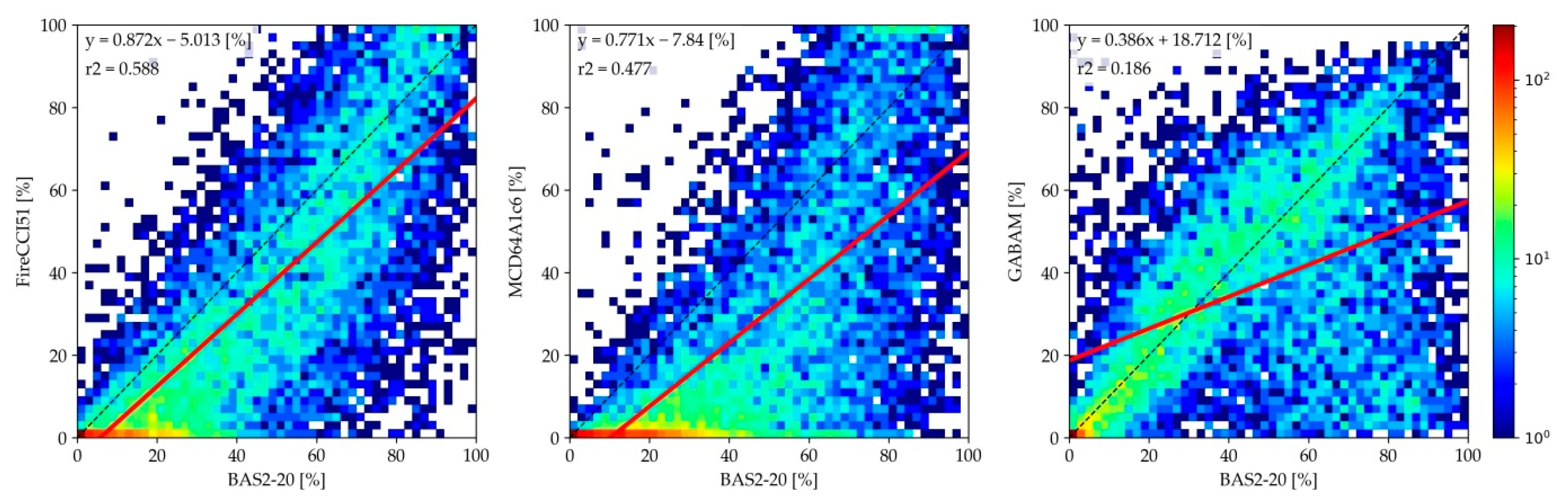
The 3 test sites from Africa, Central America, and Siberia were covered by 122 MGRS tiles in total, with 1464 monthly BA maps in total processed for the whole year 2019. The process took around 5.5 days to process, or 5.4 min per monthly BA map on average. The results obtained from this algorithm and from global products at the test site from Africa are shown in Figure 16. A total of 144,000 km2 were burned in total in 2019 at this site according to our algorithm, while this amount was lower in the case of FireCCI51 and GABAM (between 110,000 and 112,000 km2), and only 87,000 km2 were detected by MCD64A1. The largest differences are seen in the northeastern corner of the site, where many areas burned around November—according to BAS2-20—were omitted by all global products. Most large fire patches detected were consistent across all products, although the smallest fires were only mapped by BAS2-20 and GABAM. The scatter plots between burned fractions and regression lines in Figure 17 point to the same trend, since most cells have higher burned fractions in BAS2-20 than in global products. Spatially, the most similar patterns were found between BAS2-20 and FireCCI51 with the highest values for the slope of the regression line (0.872) and r2 (0.588), followed by MCD64A1 (0.771 and 0.477, respectively), and with the lowest correlation being for GABAM (slope and r2 below 0.4 and 0.2).
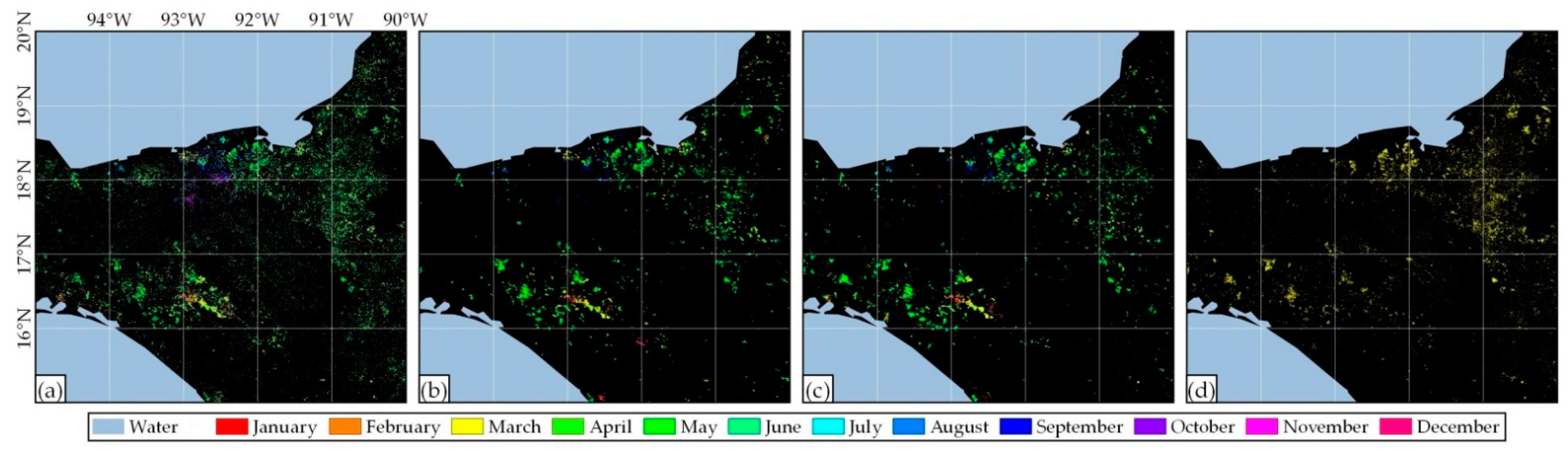
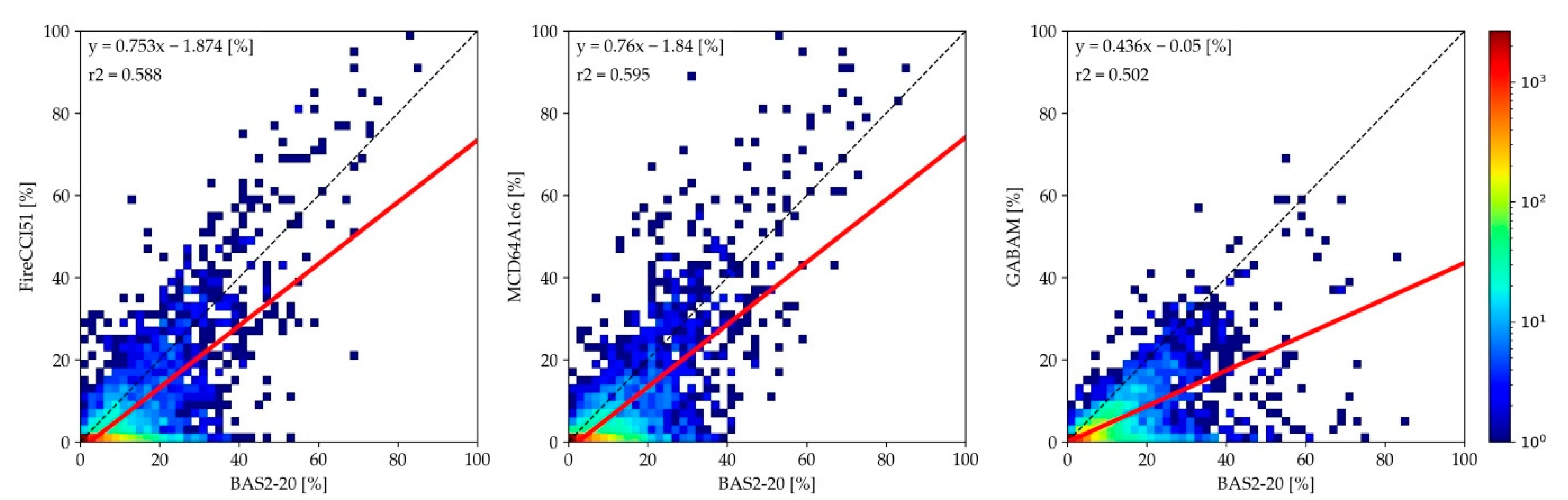
The same analysis at the test site from Central America is shown in Figure 18 and Figure 19. More than 12,800 km2 of BA were detected in 2019 according to BAS2-20, followed by both MODIS-derived products with only half the surface (between 6000 and 6200 km2), and GABAM with 5500 km2. The largest differences were found in areas affected by small size fires. Very similar results were obtained for FireCCI51 and MCD64A1 (slopes between 0.75 and 0.76, and r2 around 0.59) when comparing their BA fractions with BAS2-20. At this test site, GABAM again showed the lowest correlation.
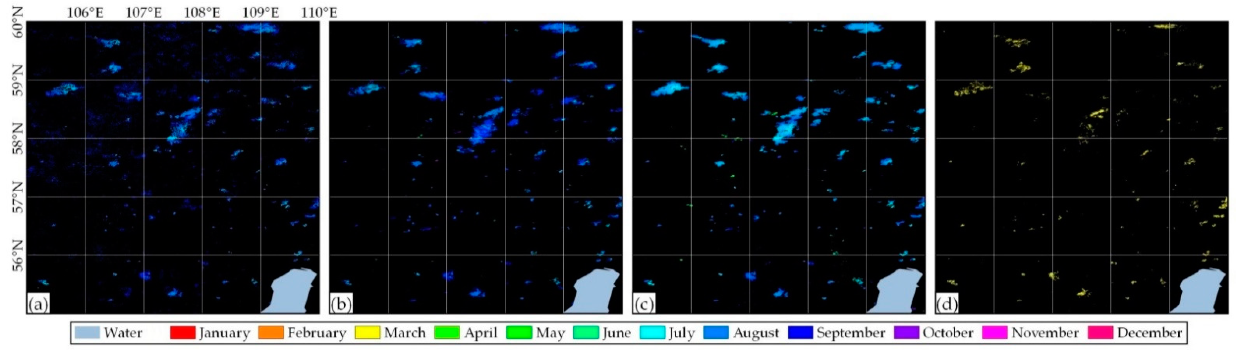
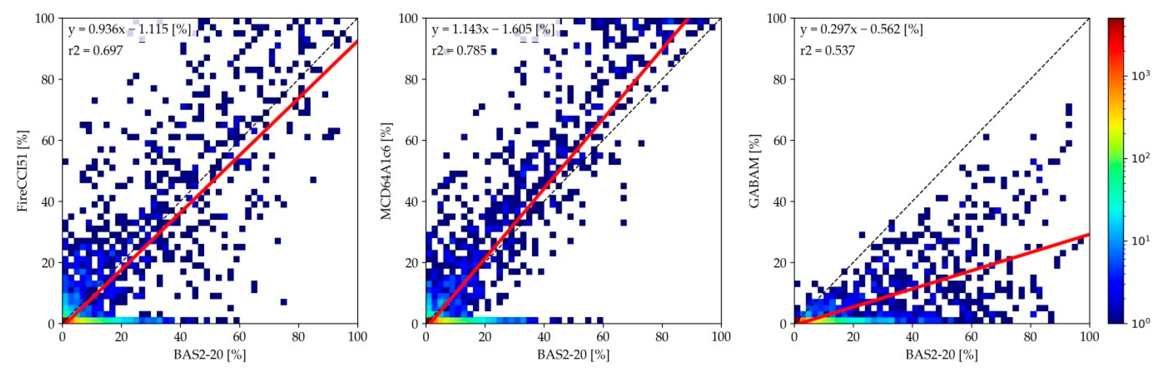
Figure 20 and Figure 21 show the results from the third site in Siberia. Detected burned surfaces by global products at coarse resolution and our algorithm differed less than at other sites, with 6300 km2, 4500 km2, and 5200 km2 found for BAS2-20, FireCCI51, and MCD64A1, respectively; GABAM only detected 1200 km2. Higher correlations with FireCCI51 and MCD64A1 than at the other test sites were found at this one (r2 of 0.697 and 0.785, respectively). The fact of the slope being higher than 1 between BAS2-20 and MCD64A1 indicates an underestimation of BA by our algorithm in boreal forests. The largest differences between BAS2-20 and coarse-resolution products were observed in the northwestern quarter of the site, where BAS2-20 incorrectly detected the decline of reflectance as having been burned at the end of summer in August and September.
4. Discussion
This paper presents a preliminary global automatic algorithm for BA detection at medium resolution, based on the MODIS active fire product MCD14DL and primarily on either Sentinel-2 (S2) or Landsat data. This is the only global BA algorithm based on S2 images so far, since only Landsat imagery has been used globally before [22], and algorithms with S2 data have been limited to national or continental scales [18,29,30,31]. Moreover, BA can be detected at both 20 and 10 m when using this dataset, even though the latter resolution has not proven to be more accurate. The algorithm is completely flexible when selecting the S2 or Landsat dataset and resolution, making it possible to produce BA in any year at the desired resolution, if S2 or Landsat datasets are available. BA from 2000 onwards can be processed with Landsat data at 30 m; previous years cannot be processed by this algorithm, despite Landsat images being available, because of the lack of MODIS hotspots for those dates. BA from 2016 onwards can also be processed at 10 or 20 m using S2 data; processing year 2015 with S2 data is possible but discouraged, because of the low number of available scenes (Figure 1).
The algorithm’s main process involves sampling some burned candidate pixels (BC) around MODIS hotspots, and then classifying the image series in burn probabilities based on spectral characteristics of these candidate pixels and detecting burned areas and dates by analyzing their temporal trend. Using an active fire product to identify some BC pixels and using these to classify images is not a novel feature, since this is already done by most global or continental BA algorithms [11,13,15,16,18,32], even though many other studies do not use hotspots to identify burned areas [10,22], especially at regional scales [25,26,27,28,29,31]. However, this is one of the first studies at non-coarse resolution that analyze the temporal evolution of spectral signals in a time series in order to establish the earliest possible detection date, as well as requiring that a burned spectral signal continue on post-fire dates [27,29,31]; the temporal consistency requirement of unburned and burned signals before and after the fire improves BA detection by avoiding possible commissions unrelated to fires, such as clouds, cloud shadows, or flooding. This approach is similar to the way some global algorithms at coarse resolution perform [10,11]. On the other hand, most BA algorithms at medium resolution either detect burned pixels on one post-fire date [63], analyze spectral changes between two single dates [18,30], search for anomalies in comparison with a multi-annual average [28], or classify every image in the time series but then just select the date with the highest probability [22,25,26], but none of them verify whether the burned signal remains after the fire.
Unburned and burned pixels at medium resolution are usually classified either by a machine-learning approach [22,26,27,31,39], decision trees [32], thresholding [29], or by logistic regression [18]. Since a machine-learning approach in a time series focus was too memory-consuming in GEE, logistic functions were used instead by this algorithm, which allowed there to be a continuous transition between unburned and burned categories. This is often followed by a two-phase strategy to balance commissions and omissions at the end of the algorithm, first identifying burned seeds and then growing regions around them. However, the process was too heavy and exceeded GEE’s user memory limits, even though several approaches were tested. Finally, an object-oriented image analysis focus was implemented using the SNIC algorithm, segmenting the burn probability and retaining the clusters with a mean probability higher than 50%.
The proposed algorithm is highly dependent on active fire products, which are required in the second step of the algorithm to identify BC pixels. Several active fire products have been developed and released in the scientific community, with the most prominent being those obtained from MODIS data at 1000 m, and from the VIIRS sensor at 375 m. Unfortunately, there is only one active fire product loaded in GEE, the near-real-time MCD14DL [52], and not the standard data product, which is internally consistent and well calibrated. FIRMS warns that the dataset is not considered to be of scientific quality [93] and, therefore, only hotspots with a confidence level over 80% are selected to overcome this limitation. Most other global BA algorithms also rely on active fire products but, since they are not limited to the products available in GEE, usually use the standard MCD14ML product processed by the University of Maryland [94,95,96], which is a further-developed and more accurate active fire product than MCD14DL [12,13,16].
Using the near-real-time and non-standard product is a significant limitation of the algorithm. MODIS hotspots have been shown to be reliable in detecting actual BA, although detection of smaller fires is limited, and show low commission errors in all land covers except in urban areas, especially related to industrial heat sources [97]. Although our algorithm masks urban areas before identifying BC pixels, the spatial disagreement between the LC product and S2 or Landsat images generate residual unmasked urban areas where BC pixels can be identified, increasing commission errors. A crucial issue when developing and optimizing our algorithm was defining the limit where small fires were to be detected or BC pixels were considered insufficient, owing to lack of sufficient hotspots. Two empirical thresholds were used for the surface covered by hotspots and by the BC pixels (detailed at the end of Section 2.2.2). However, some tiles may omit all burned areas because the BC pixels were considered to be insufficient, while in some others the algorithm may detect enough BC pixels located in falsely detected hotspots causing significant commissions.
The quality assurance of the algorithm has been divided into three exercises. First, the BA results were compared with reference data derived from Sentinel-2 images at 10 m, by analyzing 369 pairs of images and located at 50 sites selected by stratified random sampling. The sampling process took into account both the predominant biome present in each sampling unit and the fire activity; image availability and cloud presence were also checked to obtain meaningful long-period samples. The preliminary algorithm showed higher omissions (27–35%) than commission errors (9–11%). It should be noted that there is a bias here since both the BA product at 10 and 20 m (BAS2-10 and BAS2-20) and the reference data were derived from the same dataset (S2 images). However, the BA product at 30 m (BAL-30) was generated from a fully independent dataset (Landsat images), and the results suggest the robust performance of the algorithm with omissions and commissions of 35% and 11%, respectively. When processing S2 images from 2016 onwards, the algorithm can detect BA at both 20 and 10 m of spatial resolution. According to QA, the product at 10 m performed only slightly better than the 20 m resolution, with omissions and commissions being only 1.1% and 0.3% lower. This is caused mainly by the way the static probabilities are computed, because it consists of a weighted average comprising four variables where NBR2 and MIRBI (at 20 m) tend to carry more weight than NIR and NBR (at 10 m). Moreover, processing BAS2-10 maps at the 50 QA sites took longer on average than for BAS2-20 maps (5.9 vs. 4.2 min per monthly BA map), which suggests that the 20 m resolution is more suitable when processing BA from S2 data. Accuracy metrics showed much better results for this algorithm than for existing global BA products at coarse resolution, especially in terms of omissions, which were reduced from over 50% to 35% with Landsat data at 30 m, or 27–28% with S2; commissions also decreased, albeit less significantly (Table 5). These results coincide with the trend observed for other global or continental BA products at medium resolution such as FireCCISFD11 and GABAM [18,22], where a greater decrease was found for omissions than for commissions, when compared with products at coarse resolution.
The second exercise computed the reporting accuracy for BA detection. MCD64A1 was the first product when detecting burned pixels after they had actually burned, followed by FireCCI51, BAS2-10 and BAS2-20, and BAL-30 (Figure 15). However, taking into account the revisit time of each satellite, our algorithm detected between 81–84% of the burned areas in the first acquired image after the fire (the first 5 days for BAS2-10 and BAS2-20, or the first 8 days for BAL-30), while products obtained from MODIS data, with an image every day, detected 78% (MCD64A1) or 32% (FireCCI51) after the first day. It should be mentioned that MCD64A1 at 500 m detects 53% of BA the exact same day as the active fire was recorded.
The third exercise was applied to three larger test sites of 5 × 5 degrees (about 550 × 550 km2), where our BA results were compared with existing global BA products to assess the quality of the product. The comparison showed good concordance with FireCCI51 and MCD64A1, especially at the test site in boreal forests, Siberia, where highest values for r2 and slopes closest to 1 were obtained. In Africa and Central America our BAS2-20 detected a larger burned surface, since both products at coarse resolution failed to identify small fires; however, they managed to detect larger BA. GABAM, in contrast, showed significant omissions when compared to other products at all three test sites, despite its medium spatial resolution at 30 m. This may have been caused by the way its algorithm works, since it is based on a comparison between two consecutive years, selecting the date with the strongest burned signal from each year [22] and may also omit burned pixels that had already burned the previous year. The total burned surface in 2019 was 163,000 km2 at these sites, according to BAS2-20; this means an increase in BA of 35% when compared with FireCCI51 (121,000 km2), or up to 65% if compared with MCD64A1 (99,000 km2).
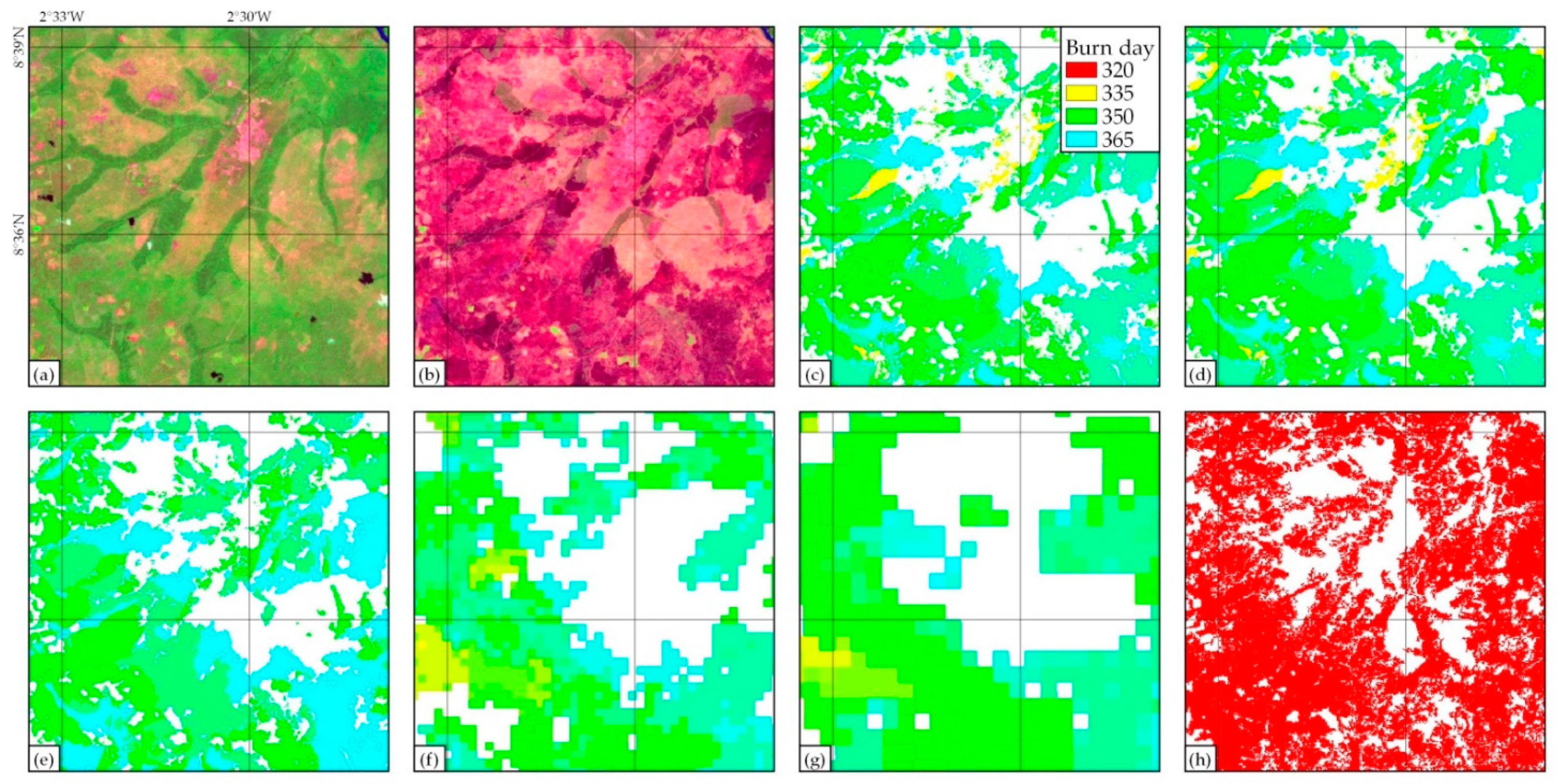
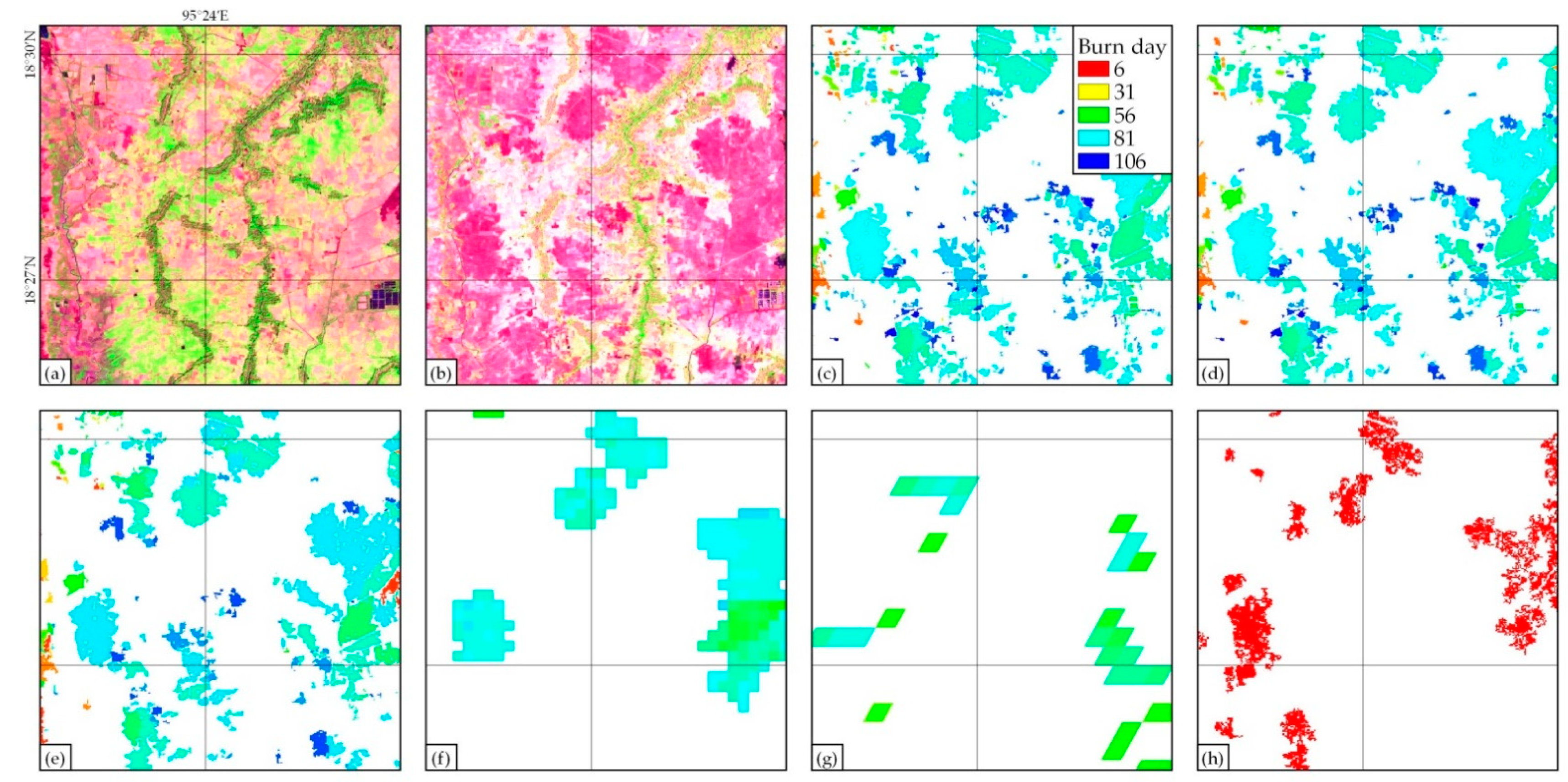
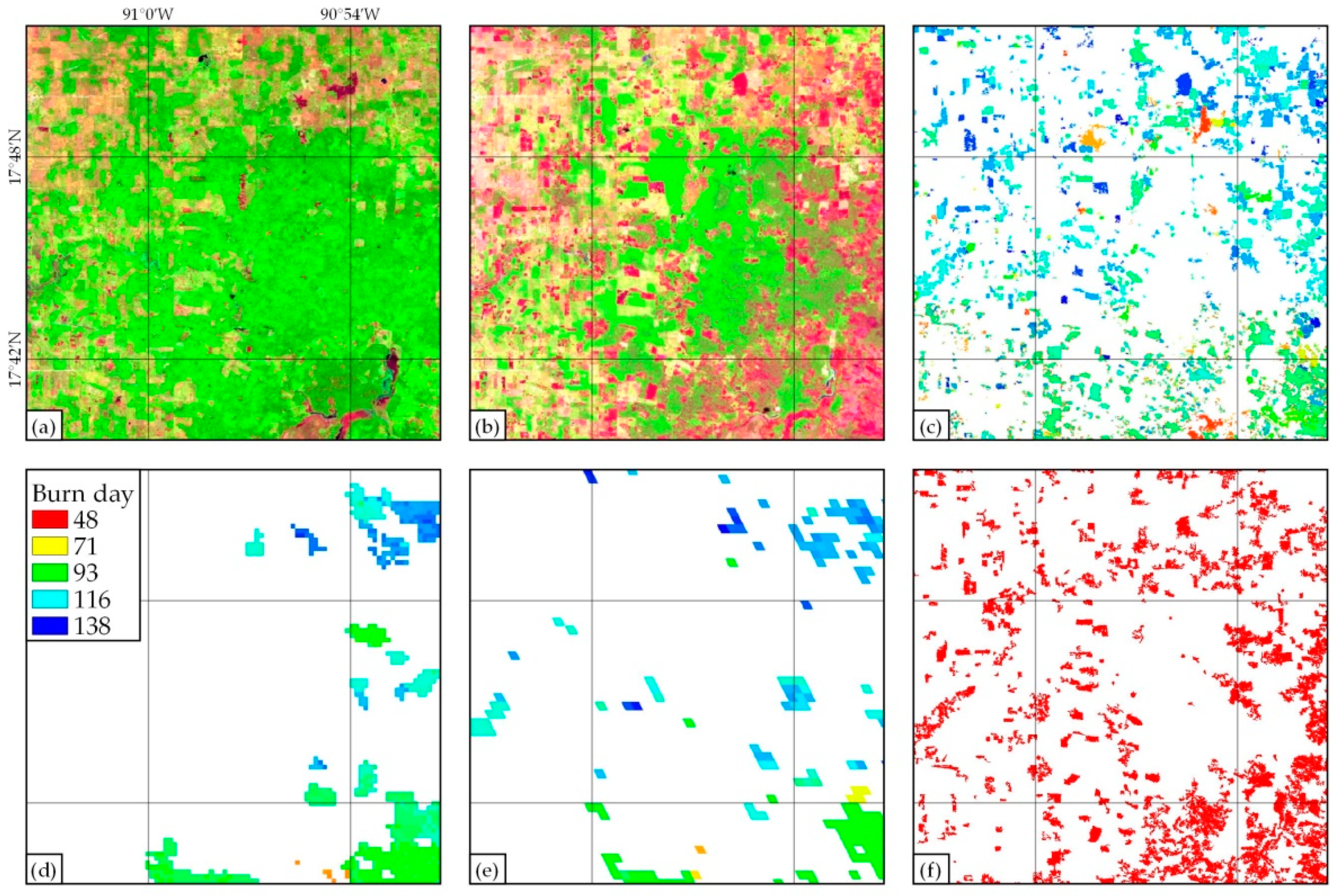
The performance of each product is illustrated in three representative sample areas located at QA site 30PWQ between Ghana and the Ivory Coast (Figure 22), QA site 46QGF in Myanmar (Figure 23) and the test site from Central America (Figure 24). BAS2-10, BAS2-20, and BAL-30 maps (in QA areas 30PWQ and 46QGF) detected practically the same BA, with very few differences, despite being at three different spatial resolutions and being derived from two independent datasets. However, products at coarser resolution omitted most small fires in all three sample areas, especially in 46QGF and Central America where most BA are small and dispersed. GABAM seems to have detected as much burned area as our algorithm in 30PWQ and Central America, but omitted a significant amount of BA in 46QGF, with similar results to those obtained by MODIS BA products despite its higher spatial resolution. There are also some BA in QA area 30PWQ that were only detected by GABAM, which may not actually be errors, but rather areas that had burned at another time of the year, since the burning date is unknown in GABAM and BA from the whole year 2019 are shown. The dates when BA were detected are also very similar, with coarse-resolution products generally identifying burned pixels some days earlier, although a few areas seem to have been detected first by BAS2-10 and BAS2-20 in tile 30PWQ.
According to the exercises for quality assurance, three main sources were found for commissions. One was partially caused by misclassifications in the land-cover map derived from MODIS data at 500 m (the IGBP classification from product MCD12Q1). The proposed BA algorithm applies many restrictions in croplands to avoid commissions, although not all croplands are correctly identified on the LC map. Many agricultural fields were found to be classified as grasslands, so they did not receive the restrictions that needed to be applied on croplands and therefore recently harvested fields were mapped as having burned. This is the reason most commissions in the QA are in grasslands, as shown in Figure 14—they actually belong to croplands. This issue could be solved if a more accurate and higher-resolution LC map were used, such as the Copernicus Land-Cover map [54], which is already available in GEE but not used by this algorithm because it does not cover as many years as the MCD12Q1 product. The second main source for the detected commissions is related to reporting accuracy. Especially in the case of BAL-30 maps obtained from Landsat data, acquisition dates did not coincide exactly with the RD period, and areas already burned on the first date, which were not part of the BA in the reference data, might be observed later in Landsat data. Since these areas appear as unburned in the RD but burned in BAL-30, they were labeled as commissions. To a lesser extent, BAS2-10 and BAS2-20 maps obtained from S2 data also displayed this type of commission, albeit in this case caused by a delay in the detection of the algorithm: around 15% of the total committed area among the 50 QA sites was detected in just one site (tile 30NYP, located in Ghana), and was caused by this delay in detection dates. The RP tool from BAMT used for reference data creation [41] and the BA algorithm presented here do not use exactly the same approach for cloud masking, and this causes areas to be observed as burned for the first time on different dates. Despite being estimated as commissions in this QA, these areas are actually not committed. A third source of commissions was found at the site from Siberia. Boreal forests were found to suffer a decrease in reflectance at the end of summer in September, and the vegetation spectral signal turned out to be similar to that of BA. If a continuous observation of the ground is possible, then the change would seem to be gradual and not classified as BA, although low observability due to high cloud coverage may result in this change appearing sudden, in which case these areas will be committed as burned.
As for omissions, another three sources were identified, with the first two affecting croplands and forests, respectively. As mentioned previously, several restrictions are applied on croplands to reduce usual commissions, since agricultural fields after harvesting and burned areas evidence similar spectral characteristics and are difficult to discriminate. These restrictions succeeded in reducing commissions considerably in croplands, but at the same time caused an increase in omissions. The second cause for omissions affects forests and is in MGRS tiles where areas were burned in both forests and other land covers. Because most burned forests display several degrees of burn severity, the BC pixels in the sampling step of the algorithm tend to gather in forested areas with high burn severity. Therefore, forests with medium to low burn severity are generally not well represented in the samples, and since these forested areas are closer to the unburned distribution in the samples, they are usually omitted in the final BA map. A third origin for omissions, albeit a less significant one, was found to be related to reporting accuracy, since some BA were detected after the last date in the RD period and labeled as omitted areas. Even though it has not been observed in the QA areas or at test sites, there could also be a fourth type of omission. To detect a burned pixel, the algorithm requires at least one previous and one further subsequent observation of the pixel, although one of these may be missing due to few available images or persistent clouds. In this case, omissions may increase considerably, even in areas that were labeled as having been observed in the exported BA map. This is likeliest to happen in tropical regions, where over 70% of Landsat scenes have been observed to be covered by clouds [98] and vegetation recovers in a few weeks after the fire [71,72]; in boreal regions, on the contrary, fire scars remain for several years [99,100], which makes it easier to detect BA even with persistent clouds.
Finally, the authors would like to note the importance of Google Earth Engine, a cloud-computing platform that enables its data catalogs to be accessed with huge processing capabilities. The use of GEE avoids the need for user technical expertise in information technology, and previously required enormous capacities for data acquisition and storage [35]. In this study, processing dense data series to detect BA proved feasible at high speeds, taking just 4–6 min on average per monthly BA map over 110 × 110 km2 at 10, 20, or 30 m of spatial resolution. However, several limitations were also found when designing and implementing the algorithm on the platform. The most challenging job was finding an efficient approach to compare individual images, since iterating on a list of images was found to be quite memory-consuming for our algorithm implementation. Even though large data series can be handled, iterative analyses slowed down the process considerably—especially when computing Pdy maps, where every date needed to be compared to several previous and following images—and this required a reduction in data. Several filters were applied to the original list of images until no more than 50 images remained, so that our algorithm was able to conclude the BA detection. The platform also proved to be limited for patch and object identification, with the main limitation being a maximum size of 1024 pixels per patch, making it impossible to identify burned areas larger than 10, 41, or 92 ha, depending on spatial resolution (10, 20, or 30 m). This was tried by way of implementation of a two-phase strategy for seed identification and region growing at the end of the algorithm to reduce commissions, but was not achieved; similarly, other approaches such as spatial dilation and cumulative cost maps proved too time-consuming for GEE, as mentioned previously. The last issue was found when computing image statistics such as Otsu thresholds or sampling pixel values, which again requires some processing capacity; this can be solved by working at coarser scales (GEE allows extracting information at different spatial resolutions, despite the native resolution of the image), although some accuracy may be lost.
5. Conclusions
A new automatic global BA detection algorithm based on Landsat or Sentinel-2 reflectance and MODIS active fires is presented in this paper, which may be processed at three different spatial resolutions—10, 20, or 30 m—depending on whether S2 or Landsat data are chosen; this is still a preliminary algorithm, and a rigorous validation with independent data should still be done in order to statistically estimate the algorithm’s accuracy, identify error sources and therefore propose necessary modifications for the algorithm before an operational global BA detection. The new methodology involves detecting some burned candidate pixels around hotspots based on their spectral changes, using these candidate pixels to classify single images from a dense time series with burn probability values, and then analyzing the temporal evolution of these probabilities to detect BA and their dates. The algorithm was implemented in Google Earth Engine, taking advantage of its huge cloud-computing and processing capabilities; since the platform’s datasets are used exclusively, BA mapping can be extended globally to any year from 2000 up to the present.
The algorithm was processed at 50 sites from 2019 selected by a stratified random sampling, where commissions in the range of 9–11% were obtained, and omissions varied between 27–35%, while nearly 20% of commissions and over 50% of omissions were observed for existing products at coarse resolution (FireCCI51 and MCD64A1), respectively. Similarly, the algorithm was processed with Sentinel-2 data at 20 m at three larger sites, where an increase in BA of 65% was found when compared with MCD64A1, or 35% when compared with FireCCI51. This must be researched further to confirm a global trend, as it would impact on current estimations of greenhouse gas emissions into the atmosphere.
Author Contributions
E.R. developed the algorithm and generated the reference data in QA areas. A.B. supervised the process. E.R., A.B., A.I. and E.C. wrote the manuscript. All authors have read and agreed to the published version of the manuscript.
Funding
This research was funded by the Vice-Rectorate for Research of the University of the Basque Country (UPV/EHU) through a doctoral fellowship (contract no. PIF17/96).
Institutional Review Board Statement
Not applicable.
Informed Consent Statement
Not applicable.
Conflicts of Interest
The authors declare no conflict of interest.
Appendix A

Table A1.
50 QA areas selected by the stratified random sampling methodology, and their biomes, first and last dates in YYYYMMDD format (with YYYY, MM, and DD standing for the year, month, and day of month), length in days, low or high fire activity, and number of images.
Table A1.
50 QA areas selected by the stratified random sampling methodology, and their biomes, first and last dates in YYYYMMDD format (with YYYY, MM, and DD standing for the year, month, and day of month), length in days, low or high fire activity, and number of images.
| Biome | Tile | First Date | Last Date | Length (Days) | Fire Activity | Number of Images |
|---|---|---|---|---|---|---|
| Boreal forest | 49WFM | 20190617 | 20190913 | 88 | high | 5 |
| 42VWN | 20190716 | 20191004 | 80 | high | 2 | |
| Mediterranean forest | 31SEA | 20190415 | 20190902 | 140 | high | 9 |
| Others | 38RQU | 20190111 | 20190327 | 75 | high | 2 |
| 42RXT | 20190114 | 20191205 | 325 | high | 24 | |
| 42RXU | 20190114 | 20191205 | 325 | high | 25 | |
| 34JHT | 20190103 | 20191219 | 350 | low | 13 | |
| Temperate forest | 49SFC | 20190630 | 20191028 | 120 | high | 7 |
| 56HLJ | 20190101 | 20191231 | 364 | high | 14 | |
| 16SBF | 20190317 | 20191102 | 230 | high | 6 | |
| Temperate grassland and savanna | 36LVQ | 20190417 | 20191103 | 200 | high | 10 |
| 36PUQ | 20190103 | 20190403 | 90 | high | 6 | |
| 44TPP | 20190515 | 20191029 | 167 | high | 3 | |
| 37UGQ | 20190401 | 20191124 | 237 | low | 12 | |
| Tropical and subtropical savanna | 33LYE | 20190430 | 20191106 | 190 | high | 13 |
| 33LWK | 20190418 | 20190920 | 155 | high | 11 | |
| 35LNF | 20190503 | 20191109 | 190 | high | 12 | |
| 30NYP | 20190102 | 20190313 | 70 | high | 6 | |
| 35LKH | 20190501 | 20191102 | 185 | high | 11 | |
| 34MCV | 20190609 | 20190917 | 100 | high | 7 | |
| 31PCN | 20191016 | 20191230 | 75 | high | 6 | |
| 37LDD | 20190801 | 20191204 | 125 | high | 10 | |
| 36LWH | 20190708 | 20191105 | 120 | high | 8 | |
| 37LDE | 20190523 | 20191119 | 180 | high | 10 | |
| 35NPF | 20190106 | 20190312 | 65 | high | 6 | |
| 36MVS | 20190522 | 20191014 | 145 | high | 10 | |
| 55LBC | 20190507 | 20191213 | 220 | high | 8 | |
| 35NPJ | 20190923 | 20191227 | 95 | high | 5 | |
| 30PWQ | 20191116 | 20191231 | 45 | high | 5 | |
| 34PHR | 20191029 | 20191228 | 60 | high | 6 | |
| 33MXT | 20190607 | 20190831 | 85 | low | 6 | |
| 52LHJ | 20190127 | 20191223 | 330 | low | 8 | |
| 30PWR | 20190110 | 20190420 | 100 | low | 8 | |
| 34KCD | 20190124 | 20191210 | 320 | low | 15 | |
| 21KYR | 20190916 | 20191230 | 105 | low | 4 | |
| 31PBQ | 20190117 | 20190407 | 80 | low | 4 | |
| 34KBC | 20190107 | 20191213 | 340 | low | 10 | |
| 34PCU | 20190113 | 20190428 | 110 | low | 5 | |
| 37PDP | 20190815 | 20191228 | 135 | low | 5 | |
| Tropical forest | 46QFL | 20190101 | 20190531 | 150 | high | 13 |
| 28PGT | 20190102 | 20190527 | 145 | high | 10 | |
| 47QLC | 20190113 | 20190428 | 105 | high | 8 | |
| 46QFG | 20190101 | 20190426 | 115 | high | 9 | |
| 21MZP | 20190701 | 20190830 | 60 | high | 4 | |
| 46QGF | 20190101 | 20190421 | 110 | high | 10 | |
| 48PVU | 20190106 | 20190411 | 95 | high | 6 | |
| 47QRA | 20190117 | 20190422 | 95 | high | 9 | |
| 21LXH | 20190427 | 20191004 | 160 | low | 7 | |
| 23LQF | 20190422 | 20191113 | 205 | low | 4 | |
| 20LKN | 20190509 | 20190916 | 130 | low | 2 |
Table A2.
Accuracy measures for our algorithm at 3 spatial resolutions and for 2 global BA products by QA site: commissions, omissions, and Dice coefficients, all expressed in percentages. A dash in all 3 of the accuracy metrics means that no BA was detected by the algorithm or product, nor in the reference data.
| MGRS Tile | BAS2-10 | BAS2-20 | BAL-30 | FireCCI51 | MCD64A1 | ||||||||||
|---|---|---|---|---|---|---|---|---|---|---|---|---|---|---|---|
| CE | OE | DC | CE | OE | DC | CE | OE | DC | CE | OE | DC | CE | OE | DC | |
| 49WFM | 77.6 | 0.7 | 36.5 | 79.7 | 0.4 | 33.7 | 46.0 | 3.6 | 69.2 | 20.0 | 22.7 | 78.7 | 8.4 | 12.4 | 89.6 |
| 42VWN | 100.0 | 0.0 | 0.0 | 100.0 | 0.0 | 0.0 | - | - | - | - | - | - | - | - | - |
| 31SEA | 2.7 | 30.5 | 81.1 | 2.5 | 30.6 | 81.1 | 3.3 | 36.1 | 77.0 | 41.8 | 36.4 | 60.8 | 32.8 | 49.4 | 57.7 |
| 38RQU | - | - | - | - | - | - | - | - | - | - | - | - | - | - | - |
| 42RXT | 14.2 | 95.4 | 8.8 | 15.8 | 96.3 | 7.1 | 13.6 | 93.4 | 12.2 | 28.2 | 87.0 | 22.0 | 41.9 | 83.7 | 25.4 |
| 42RXU | 6.6 | 99.6 | 0.9 | 2.6 | 99.5 | 0.9 | 2.6 | 100.0 | 0.1 | 12.0 | 85.4 | 25.0 | 6.7 | 96.3 | 7.2 |
| 34JHT | - | - | - | - | - | - | - | - | - | - | - | - | - | - | - |
| 49SFC | 0.0 | 100.0 | 0.0 | 0.0 | 100.0 | 0.0 | 0.0 | 100.0 | 0.0 | 0.0 | 100.0 | 0.0 | 0.0 | 100.0 | 0.0 |
| 56HLJ | 10.5 | 21.3 | 83.7 | 12.2 | 22.1 | 82.6 | 5.2 | 90.5 | 17.3 | 39.1 | 73.9 | 36.5 | 64.3 | 38.6 | 45.2 |
| 16SBF | 34.8 | 90.2 | 17.1 | 28.5 | 86.5 | 22.8 | 79.6 | 95.6 | 7.3 | 39.5 | 74.0 | 36.4 | 93.7 | 55.2 | 11.0 |
| 36LVQ | 6.2 | 14.6 | 89.4 | 6.1 | 16.0 | 88.6 | 6.9 | 23.5 | 84.0 | 8.0 | 61.0 | 54.7 | 6.7 | 71.8 | 43.4 |
| 36PUQ | 0.2 | 2.9 | 98.4 | 0.3 | 2.9 | 98.4 | 1.1 | 3.5 | 97.7 | 3.4 | 15.0 | 90.4 | 8.1 | 6.5 | 92.7 |
| 44TPP | - | - | - | - | - | - | - | - | - | - | - | - | - | - | - |
| 37UGQ | 2.2 | 69.3 | 46.7 | 2.3 | 70.1 | 45.7 | 1.8 | 75.4 | 39.4 | 27.9 | 98.6 | 2.7 | 24.8 | 92.7 | 13.4 |
| 33LYE | 1.5 | 13.9 | 91.9 | 1.7 | 14.5 | 91.4 | 2.4 | 21.0 | 87.3 | 13.9 | 51.6 | 62.0 | 15.9 | 55.9 | 57.9 |
| 33LWK | 3.3 | 1.5 | 97.6 | 3.4 | 1.7 | 97.4 | 4.6 | 3.7 | 95.8 | 8.7 | 3.6 | 93.8 | 7.3 | 23.8 | 83.7 |
| 35LNF | 2.2 | 50.7 | 65.5 | 2.3 | 52.5 | 64.0 | 3.7 | 54.6 | 61.7 | 20.2 | 38.4 | 69.6 | 19.6 | 53.7 | 58.8 |
| 30NYP | 23.8 | 12.0 | 81.7 | 23.3 | 13.9 | 81.1 | 22.9 | 27.4 | 74.7 | 38.9 | 53.5 | 52.8 | 20.2 | 92.6 | 13.6 |
| 35LKH | 2.3 | 15.3 | 90.8 | 2.8 | 16.2 | 90.0 | 6.6 | 22.3 | 84.8 | 18.8 | 37.2 | 70.9 | 16.0 | 53.4 | 59.9 |
| 34MCV | 12.1 | 30.7 | 77.5 | 12.3 | 40.9 | 70.6 | 31.3 | 68.9 | 42.8 | 54.3 | 93.8 | 10.9 | 38.2 | 96.6 | 6.4 |
| 31PCN | 0.5 | 29.6 | 82.5 | 0.6 | 29.6 | 82.4 | 0.9 | 32.0 | 80.7 | 12.5 | 1.1 | 92.9 | 10.8 | 5.2 | 91.9 |
| 37LDD | 6.8 | 37.0 | 75.2 | 7.4 | 39.6 | 73.1 | 14.4 | 60.5 | 54.0 | 25.9 | 70.4 | 42.3 | 27.3 | 68.4 | 44.0 |
| 36LWH | 5.8 | 11.3 | 91.4 | 6.2 | 11.8 | 90.9 | 10.3 | 20.3 | 84.4 | 22.5 | 44.6 | 64.6 | 16.7 | 71.6 | 42.4 |
| 37LDE | 2.8 | 17.8 | 89.1 | 2.8 | 18.5 | 88.6 | 4.8 | 33.3 | 78.4 | 12.5 | 39.7 | 71.4 | 12.3 | 33.9 | 75.4 |
| 35NPF | 11.8 | 35.0 | 74.8 | 12.4 | 36.1 | 73.9 | 22.2 | 31.8 | 72.7 | 46.2 | 56.5 | 48.1 | 32.5 | 88.3 | 20.0 |
| 36MVS | 1.8 | 15.7 | 90.7 | 1.9 | 16.5 | 90.2 | 2.2 | 27.2 | 83.5 | 9.5 | 20.8 | 84.5 | 8.7 | 33.0 | 77.3 |
| 55LBC | 5.6 | 11.7 | 91.2 | 5.6 | 11.7 | 91.2 | 5.9 | 18.7 | 87.2 | 15.3 | 7.0 | 88.6 | 10.3 | 24.6 | 81.9 |
| 35NPJ | 4.2 | 14.3 | 90.5 | 4.6 | 14.2 | 90.4 | 8.2 | 20.9 | 85.0 | 13.1 | 56.3 | 58.1 | 15.0 | 57.7 | 56.5 |
| 30PWQ | 3.8 | 6.1 | 95.0 | 4.2 | 6.0 | 94.9 | 5.7 | 6.9 | 93.7 | 23.1 | 32.0 | 72.2 | 17.6 | 35.0 | 72.7 |
| 34PHR | 10.4 | 27.3 | 80.2 | 11.6 | 23.2 | 82.2 | 24.2 | 22.8 | 76.5 | 46.8 | 72.9 | 35.9 | 41.1 | 91.5 | 14.9 |
| 33MXT | 4.6 | 42.7 | 71.6 | 4.4 | 45.8 | 69.2 | 8.1 | 64.6 | 51.1 | 40.2 | 87.8 | 20.2 | 60.7 | 89.5 | 16.6 |
| 52LHJ | 22.2 | 2.3 | 86.6 | 18.8 | 3.0 | 88.4 | 65.6 | 3.9 | 50.7 | 13.0 | 2.3 | 92.0 | 7.2 | 10.3 | 91.2 |
| 30PWR | 12.2 | 61.5 | 53.5 | 12.8 | 66.6 | 48.3 | 52.8 | 73.0 | 34.3 | 98.2 | 100.0 | 0.1 | 0.0 | 100.0 | 0.0 |
| 34KCD | 4.7 | 11.9 | 91.5 | 5.6 | 12.5 | 90.8 | 9.7 | 20.0 | 84.8 | 0.0 | 100.0 | 0.0 | 20.4 | 69.1 | 44.5 |
| 21KYR | 99.7 | 95.6 | 0.6 | 99.9 | 99.1 | 0.1 | 96.3 | 26.6 | 7.0 | 0.0 | 100.0 | 0.0 | 0.0 | 100.0 | 0.0 |
| 31PBQ | 0.0 | 100.0 | 0.0 | 0.0 | 100.0 | 0.0 | 0.0 | 100.0 | 0.0 | 0.0 | 100.0 | 0.0 | 0.0 | 100.0 | 0.0 |
| 34KBC | - | - | - | - | - | - | - | - | - | - | - | - | - | - | - |
| 34PCU | 4.9 | 32.0 | 79.3 | 6.0 | 34.5 | 77.2 | 8.5 | 41.4 | 71.4 | 0.0 | 100.0 | 0.0 | 0.0 | 100.0 | 0.0 |
| 37PDP | 0.0 | 100.0 | 0.0 | 0.0 | 100.0 | 0.0 | 0.0 | 100.0 | 0.0 | 0.0 | 100.0 | 0.0 | 0.0 | 100.0 | 0.0 |
| 46QFL | 10.8 | 44.3 | 68.6 | 11.0 | 45.5 | 67.6 | 12.7 | 53.0 | 61.1 | 0.0 | 100.0 | 0.0 | 24.9 | 68.4 | 44.5 |
| 28PGT | 4.9 | 33.0 | 78.6 | 5.1 | 34.8 | 77.3 | 9.0 | 44.7 | 68.8 | 24.5 | 65.0 | 47.8 | 31.0 | 55.1 | 54.4 |
| 47QLC | 10.2 | 51.8 | 62.8 | 9.9 | 57.4 | 57.9 | 9.8 | 71.1 | 43.8 | 0.0 | 100.0 | 0.0 | 31.9 | 91.7 | 14.7 |
| 46QFG | 8.5 | 58.5 | 57.1 | 7.7 | 61.6 | 54.2 | 8.9 | 70.2 | 45.0 | 33.5 | 89.1 | 18.7 | 48.4 | 68.6 | 39.1 |
| 21MZP | 5.9 | 49.6 | 65.6 | 6.2 | 50.3 | 65.0 | 13.1 | 23.8 | 81.2 | 37.0 | 23.4 | 69.1 | 34.3 | 39.7 | 62.9 |
| 46QGF | 4.3 | 22.6 | 85.6 | 4.7 | 27.6 | 82.3 | 15.5 | 33.1 | 74.7 | 40.1 | 70.4 | 39.7 | 41.2 | 88.0 | 20.0 |
| 48PVU | 22.1 | 42.4 | 66.2 | 22.2 | 45.4 | 64.2 | 28.3 | 57.0 | 53.8 | 36.1 | 95.0 | 9.3 | 38.7 | 96.1 | 7.3 |
| 47QRA | 33.1 | 41.5 | 62.4 | 31.9 | 56.0 | 53.5 | 26.4 | 76.3 | 35.9 | 0.0 | 100.0 | 0.0 | 0.0 | 100.0 | 0.0 |
| 21LXH | 82.3 | 31.5 | 28.2 | 80.7 | 32.8 | 30.0 | 89.7 | 38.9 | 17.6 | 0.0 | 100.0 | 0.0 | 0.0 | 100.0 | 0.0 |
| 23LQF | 98.9 | 50.2 | 2.2 | 99.2 | 59.6 | 1.6 | 99.4 | 68.9 | 1.3 | 0.0 | 100.0 | 0.0 | 0.0 | 100.0 | 0.0 |
| 20LKN | 100.0 | 0.0 | 0.0 | 100.0 | 0.0 | 0.0 | 100.0 | 0.0 | 0.0 | - | - | - | - | - | - |
References
- GCOS. The Global Observing System For Climate: Implementation Needs GCOS-200 (GOOS-214). Available online: https://library.wmo.int/doc_num.php?explnum_id=3417 (accessed on 25 October 2021).
- Bowman, D.M.J.S.; Balch, J.K.; Artaxo, P.; Bond, W.J.; Carlson, J.M.; Cochrane, M.A.; D’Antonio, C.M.; DeFries, R.S.; Doyle, J.C.; Harrison, S.P.; et al. Fire in the Earth System. Science 2009, 324, 481–484. [Google Scholar] [CrossRef]
- Van Der Werf, G.R.; Randerson, J.T.; Giglio, L.; Van Leeuwen, T.T.; Chen, Y.; Rogers, B.M.; Mu, M.; Van Marle, M.J.E.; Morton, D.C.; Collatz, G.J.; et al. Global fire emissions estimates during 1997–2016. Earth Syst. Sci. Data 2017, 9, 697–720. [Google Scholar] [CrossRef] [Green Version]
- Roos, C.I.; Scott, A.C.; Belcher, C.M.; Chaloner, W.G.; Aylen, J.; Bird, R.B.; Coughlan, M.R.; Johnson, B.R.; Johnston, F.H.; McMorrow, J.; et al. Living on a flammable planet: Interdisciplinary, cross-scalar and varied cultural lessons, prospects and challenges. Philos. Trans. R. Soc. B Biol. Sci. 2016, 371, 20150469. [Google Scholar] [CrossRef] [PubMed] [Green Version]
- Forkel, M.; Dorigo, W.; Lasslop, G.; Teubner, I.; Chuvieco, E.; Thonicke, K. A data-driven approach to identify controls on global fire activity from satellite and climate observations (SOFIA V1). Geosci. Model Dev. 2017, 10, 4443–4476. [Google Scholar] [CrossRef] [Green Version]
- Tansey, K.; Grégoire, J.; Stroppiana, D.; Sousa, A.; Silva, J.; Pereira, J.M.C.; Boschetti, L.; Maggi, M.; Brivio, P.A.; Fraser, R.; et al. Vegetation burning in the year 2000: Global burned area estimates from SPOT VEGETATION data. J. Geophys. Res. 2004, 109, D14S03. [Google Scholar] [CrossRef] [Green Version]
- Simon, M.; Plummer, S.; Fierens, F.; Hoelzemann, J.J.; Arino, O. Burnt area detection at global scale using ATSR-2: The GLOBSCAR products and their qualification. J. Geophys. Res. 2004, 109, D14S02. [Google Scholar] [CrossRef]
- Tansey, K.; Grégoire, J.; Defourny, P.; Leigh, R.; Pekel, J.; Van Bogaert, E.; Bartholomé, E. A new, global, multi-annual (2000–2007) burnt area product at 1 km resolution. Geophys. Res. Lett. 2008, 35. [Google Scholar] [CrossRef]
- Tansey, K.; Bradley, A.; Smets, B.; van Best, C.; Lacaze, R. The Geoland2 BioPar burned area product. In Proceedings of the EGU General Assembly Conference Abstracts, Viena, Austria, 22–27 April 2012; p. 4727. [Google Scholar]
- Roy, D.P.; Jin, Y.; Lewis, P.E.; Justice, C.O. Prototyping a global algorithm for systematic fire-affected area mapping using MODIS time series data. Remote Sens. Environ. 2005, 97, 137–162. [Google Scholar] [CrossRef]
- Giglio, L.; Loboda, T.; Roy, D.P.; Quayle, B.; Justice, C.O. An active-fire based burned area mapping algorithm for the MODIS sensor. Remote Sens. Environ. 2009, 113, 408–420. [Google Scholar] [CrossRef]
- Giglio, L.; Boschetti, L.; Roy, D.P.; Humber, M.L.; Justice, C.O. The Collection 6 MODIS burned area mapping algorithm and product. Remote Sens. Environ. 2018, 217, 72–85. [Google Scholar] [CrossRef]
- Alonso-Canas, I.; Chuvieco, E. Global burned area mapping from ENVISAT-MERIS and MODIS active fire data. Remote Sens. Environ. 2015, 163, 140–152. [Google Scholar] [CrossRef]
- Chuvieco, E.; Yue, C.; Heil, A.; Mouillot, F.; Alonso-Canas, I.; Padilla, M.; Pereira, J.M.; Oom, D.; Tansey, K. A new global burned area product for climate assessment of fire impacts. Glob. Ecol. Biogeogr. 2016, 25, 619–629. [Google Scholar] [CrossRef] [Green Version]
- Chuvieco, E.; Lizundia-Loiola, J.; Lucrecia Pettinari, M.; Ramo, R.; Padilla, M.; Tansey, K.; Mouillot, F.; Laurent, P.; Storm, T.; Heil, A.; et al. Generation and analysis of a new global burned area product based on MODIS 250 m reflectance bands and thermal anomalies. Earth Syst. Sci. Data 2018, 10, 2015–2031. [Google Scholar] [CrossRef] [Green Version]
- Lizundia-Loiola, J.; Otón, G.; Ramo, R.; Chuvieco, E. A spatio-temporal active-fire clustering approach for global burned area mapping at 250 m from MODIS data. Remote Sens. Environ. 2020, 236, 111493. [Google Scholar] [CrossRef]
- Randerson, J.T.; Chen, Y.; van der Werf, G.R.; Rogers, B.M.; Morton, D.C. Global burned area and biomass burning emissions from small fires. J. Geophys. Res. Biogeosci. 2012, 117. [Google Scholar] [CrossRef]
- Roteta, E.; Bastarrika, A.; Padilla, M.; Storm, T.; Chuvieco, E. Development of a Sentinel-2 burned area algorithm: Generation of a small fire database for sub-Saharan Africa. Remote Sens. Environ. 2019, 222, 1–17. [Google Scholar] [CrossRef]
- Ramo, R.; Roteta, E.; Bistinas, I.; van Wees, D.; Bastarrika, A.; Chuvieco, E.; van der Werf, G.R. African burned area and fire carbon emissions are strongly impacted by small fires undetected by coarse resolution satellite data. Proc. Natl. Acad. Sci. USA 2021, 118, e2011160118. [Google Scholar] [CrossRef]
- Padilla, M.; Stehman, S.V.; Ramo, R.; Corti, D.; Hantson, S.; Oliva, P.; Alonso-Canas, I.; Bradley, A.V.; Tansey, K.; Mota, B.; et al. Comparing the accuracies of remote sensing global burned area products using stratified random sampling and estimation. Remote Sens. Environ. 2015, 160, 114–121. [Google Scholar] [CrossRef] [Green Version]
- Boschetti, L.; Roy, D.P.; Giglio, L.; Huang, H.; Zubkova, M.; Humber, M.L. Global validation of the collection 6 MODIS burned area product. Remote Sens. Environ. 2019, 235, 111490. [Google Scholar] [CrossRef] [PubMed]
- Long, T.; Zhang, Z.; He, G.; Jiao, W.; Tang, C.; Wu, B.; Zhang, X.; Wang, G.; Yin, R. 30m resolution Global Annual Burned Area Mapping based on Landsat images and Google Earth Engine. Remote Sens. 2019, 11, 489. [Google Scholar] [CrossRef] [Green Version]
- Updated 30 m Resolution Global Annual Burned Area Map—Remote Sensing of Global Change. Available online: https://vapd.gitlab.io/post/gabam/ (accessed on 11 February 2021).
- Wei, M.; Zhang, Z.; Long, T.; He, G.; Wang, G. Monitoring Landsat Based Burned Area as an Indicator of Sustainable Development Goals. Earth’s Future 2021, 9, e2020EF001960. [Google Scholar] [CrossRef]
- Hawbaker, T.J.; Vanderhoof, M.K.; Beal, Y.-J.; Takacs, J.D.; Schmidt, G.L.; Falgout, J.T.; Williams, B.; Fairaux, N.M.; Caldwell, M.K.; Picotte, J.J.; et al. Mapping burned areas using dense time-series of Landsat data. Remote Sens. Environ. 2017, 198, 504–522. [Google Scholar] [CrossRef]
- Hawbaker, T.J.; Vanderhoof, M.K.; Schmidt, G.L.; Beal, Y.J.; Picotte, J.J.; Takacs, J.D.; Falgout, J.T.; Dwyer, J.L. The Landsat Burned Area algorithm and products for the conterminous United States. Remote Sens. Environ. 2020, 244, 111801. [Google Scholar] [CrossRef]
- Goodwin, N.R.; Collett, L.J. Development of an automated method for mapping fire history captured in Landsat TM and ETM+ time series across Queensland, Australia. Remote Sens. Environ. 2014, 148, 206–221. [Google Scholar] [CrossRef]
- Liu, J.; Heiskanen, J.; Maeda, E.E.; Pellikka, P.K.E. Burned area detection based on Landsat time series in savannas of southern Burkina Faso. Int. J. Appl. Earth Obs. Geoinf. 2018, 64, 210–220. [Google Scholar] [CrossRef] [Green Version]
- Filipponi, F. Exploitation of sentinel-2 time series to map burned areas at the national level: A case study on the 2017 Italy wildfires. Remote Sens. 2019, 11, 622. [Google Scholar] [CrossRef] [Green Version]
- Llorens, R.; Sobrino, J.A.; Fernández, C.; Fernández-Alonso, J.M.; Vega, J.A. A methodology to estimate forest fires burned areas and burn severity degrees using Sentinel-2 data. Application to the October 2017 fires in the Iberian Peninsula. Int. J. Appl. Earth Obs. Geoinf. 2021, 95, 102243. [Google Scholar] [CrossRef]
- Roy, D.P.; Huang, H.; Boschetti, L.; Giglio, L.; Yan, L.; Zhang, H.H.; Li, Z. Landsat-8 and Sentinel-2 burned area mapping—A combined sensor multi-temporal change detection approach. Remote Sens. Environ. 2019, 231, 111254. [Google Scholar] [CrossRef]
- Boschetti, L.; Roy, D.P.; Justice, C.O.; Humber, M.L. MODIS–Landsat fusion for large area 30m burned area mapping. Remote Sens. Environ. 2015, 161, 27–42. [Google Scholar] [CrossRef]
- Belenguer-Plomer, M.A.; Tanase, M.A.; Chuvieco, E.; Bovolo, F. CNN-based burned area mapping using radar and optical data. Remote Sens. Environ. 2021, 260, 112468. [Google Scholar] [CrossRef]
- Stroppiana, D.; Azar, R.; Calò, F.; Pepe, A.; Imperatore, P.; Boschetti, M.; Silva, J.M.N.; Brivio, P.A.; Lanari, R. Integration of optical and SAR data for burned area mapping in Mediterranean regions. Remote Sens. 2015, 7, 1320–1345. [Google Scholar] [CrossRef] [Green Version]
- Gorelick, N.; Hancher, M.; Dixon, M.; Ilyushchenko, S.; Thau, D.; Moore, R. Google Earth Engine: Planetary-scale geospatial analysis for everyone. Remote Sens. Environ. 2017, 202, 18–27. [Google Scholar] [CrossRef]
- Hansen, M.C.; Potapov, P.V.; Moore, R.; Hancher, M.; Turubanova, S.A.; Tyukavina, A.; Thau, D.; Stehman, S.V.; Goetz, S.J.; Loveland, T.R.; et al. High-resolution global maps of 21st-century forest cover change. Science 2013, 342, 850–853. [Google Scholar] [CrossRef] [Green Version]
- Wang, L.; Diao, C.; Xian, G.; Yin, D.; Lu, Y.; Zou, S.; Erickson, T.A. A summary of the special issue on remote sensing of land change science with Google earth engine. Remote Sens. Environ. 2020, 248, 112002. [Google Scholar] [CrossRef]
- Daldegan, G.A.; Roberts, D.A.; Ribeiro, F.d.F. Spectral mixture analysis in Google Earth Engine to model and delineate fire scars over a large extent and a long time-series in a rainforest-savanna transition zone. Remote Sens. Environ. 2019, 232, 111340. [Google Scholar] [CrossRef]
- Roteta, E.; Oliva, P. Optimization of A Random Forest Classifier for Burned Area Detection in Chile Using Sentinel-2 Data. In Proceedings of the 2020 IEEE Latin American GRSS & ISPRS Remote Sensing Conference (LAGIRS), Santiago, Chile, 22–26 March 2020. [Google Scholar]
- Seydi, S.T.; Akhoondzadeh, M.; Amani, M.; Mahdavi, S. Wildfire Damage Assessment over Australia Using Sentinel-2 Imagery and MODIS Land Cover Product within the Google Earth Engine Cloud Platform. Remote Sens. 2021, 13, 220. [Google Scholar] [CrossRef]
- Roteta, E.; Bastarrika, A.; Franquesa, M.; Chuvieco, E. Landsat and Sentinel-2 Based Burned Area Mapping Tools in Google Earth Engine. Remote Sens. 2021, 13, 816. [Google Scholar] [CrossRef]
- Verhegghen, A.; Eva, H.; Ceccherini, G.; Achard, F.; Gond, V.; Gourlet-Fleury, S.; Cerutti, P. The Potential of Sentinel Satellites for Burnt Area Mapping and Monitoring in the Congo Basin Forests. Remote Sens. 2016, 8, 986. [Google Scholar] [CrossRef] [Green Version]
- Landsat Missions. Available online: https://www.usgs.gov/core-science-systems/nli/landsat (accessed on 24 January 2021).
- The Worldwide Reference System|Landsat Science. Available online: https://landsat.gsfc.nasa.gov/about/worldwide-reference-system (accessed on 13 July 2021).
- Arvidson, T.; Goward, S.; Gasch, J.; Williams, D. Landsat-7 long-term acquisition plan: Development and validation. Photogramm. Eng. Remote Sens. 2006, 72, 1137–1146. [Google Scholar] [CrossRef]
- Masek, J.G.; Vermote, E.F.; Saleous, N.E.; Wolfe, R.; Hall, F.G.; Huemmrich, K.F.; Gao, F.; Kutler, J.; Lim, T.K. A landsat surface reflectance dataset for North America, 1990–2000. IEEE Geosci. Remote Sens. Lett. 2006, 3, 68–72. [Google Scholar] [CrossRef]
- Vermote, E.; Justice, C.; Claverie, M.; Franch, B. Preliminary analysis of the performance of the Landsat 8/OLI land surface reflectance product. Remote Sens. Environ. 2016, 185, 46–56. [Google Scholar] [CrossRef] [PubMed]
- ESA. Sentinel-2. Available online: http://www.esa.int/Applications/Observing_the_Earth/Copernicus/Sentinel-2 (accessed on 24 January 2021).
- NGA. Geomatics—Coordinate Systems. Available online: https://earth-info.nga.mil/index.php?dir=coordsys&action=coordsys#tab_mgrs (accessed on 26 March 2021).
- Gascon, F.; Bouzinac, C.; Thépaut, O.; Jung, M.; Francesconi, B.; Louis, J.; Lonjou, V.; Lafrance, B.; Massera, S.; Gaudel-Vacaresse, A.; et al. Copernicus Sentinel-2A calibration and products validation status. Remote Sens. 2017, 9, 584. [Google Scholar] [CrossRef] [Green Version]
- Roy, D.P.; Boschetti, L.; Justice, C.O.; Ju, J. The collection 5 MODIS burned area product—Global evaluation by comparison with the MODIS active fire product. Remote Sens. Environ. 2008, 112, 3690–3707. [Google Scholar] [CrossRef]
- MCD14DL|Earthdata. Available online: https://earthdata.nasa.gov/earth-observation-data/near-real-time/firms/c6-mcd14dl (accessed on 24 March 2021).
- Sulla-Menashe, D.; Friedl, M. MCD12Q1 MODIS/Terra+Aqua Land Cover Type Yearly L3 Global 500 m SIN Grid V006. 2019. Available online: https://ladsweb.modaps.eosdis.nasa.gov/missions-and-measurements/products/MCD12Q1 (accessed on 25 October 2021).
- Buchhorn, M.; Lesiv, M.; Tsendbazar, N.E.; Herold, M.; Bertels, L.; Smets, B. Copernicus global land cover layers-collection 2. Remote Sens. 2020, 12, 1044. [Google Scholar] [CrossRef] [Green Version]
- Pekel, J.F.; Cottam, A.; Gorelick, N.; Belward, A.S. High-resolution mapping of global surface water and its long-term changes. Nature 2016, 540, 418–422. [Google Scholar] [CrossRef]
- Key, C.H.; Benson, N. The Normalized Burn Ratio (NBR): A Landsat TM Radiometric Measure of Burn Severity; US Geological Survey, Northern Rocky Mountain Science Center: Bozeman, MT, USA, 1999.
- García, M.J.L.; Caselles, V. Mapping burns and natural reforestation using thematic Mapper data. Geocarto Int. 1991, 6, 31–37. [Google Scholar] [CrossRef]
- Trigg, S.; Flasse, S. An evaluation of different bi-spectral spaces for discriminating burned shrub-savannah. Int. J. Remote Sens. 2001, 22, 2641–2647. [Google Scholar] [CrossRef]
- Huang, H.; Roy, D.P.; Boschetti, L.; Zhang, H.K.; Yan, L.; Kumar, S.S.; Gomez-Dans, J.; Li, J. Separability analysis of Sentinel-2A Multi-Spectral Instrument (MSI) data for burned area discrimination. Remote Sens. 2016, 8, 873. [Google Scholar] [CrossRef] [Green Version]
- van Dijk, D.; Shoaie, S.; van Leeuwen, T.; Veraverbeke, S. Spectral signature analysis of false positive burned area detection from agricultural harvests using Sentinel-2 data. Int. J. Appl. Earth Obs. Geoinf. 2021, 97, 102296. [Google Scholar] [CrossRef]
- Stroppiana, D.; Bordogna, G.; Carrara, P.; Boschetti, M.; Boschetti, L.; Brivio, P.A. A method for extracting burned areas from Landsat TM/ETM+ images by soft aggregation of multiple Spectral Indices and a region growing algorithm. ISPRS J. Photogramm. Remote Sens. 2012, 69, 88–102. [Google Scholar] [CrossRef]
- Otsu, N. A Threshold Selection Method from Gray-Level Histograms. IEEE Trans. Syst. Man Cybern. 1979, 9, 62–66. [Google Scholar] [CrossRef] [Green Version]
- Koutsias, N.; Karteris, M. Burned area mapping using logistic regression modeling of a single post-fire Landsat-5 Thematic Mapper image. Int. J. Remote Sens. 2000, 21, 673–687. [Google Scholar] [CrossRef]
- Fraser, R.H.; Fernandes, R.; Latifovic, R. Multi-temporal burned area mapping using logistic regression analysis and change metrics. In Proceedings of the IEEE International Geoscience and Remote Sensing Symposium, Toronto, ON, Canada, 24–28 June 2002; Volume 3, pp. 1486–1488. [Google Scholar]
- Pu, R.; Gong, P. Determination of burnt scars using logistic regression and neural network techniques from a single post-fire Landsat 7 ETM+ image. Photogramm. Eng. Remote Sens. 2004, 70, 841–850. [Google Scholar] [CrossRef]
- Bastarrika, A.; Chuvieco, E.; Martín, M.P. Mapping burned areas from Landsat TM/ETM+ data with a two-phase algorithm: Balancing omission and commission errors. Remote Sens. Environ. 2011, 115, 1003–1012. [Google Scholar] [CrossRef]
- Kaufman, Y.J.; Remer, L.A. Detection of Forests Using Mid-IR Reflectance: An Application for Aerosol Studies. IEEE Trans. Geosci. Remote Sens. 1994, 32, 672–683. [Google Scholar] [CrossRef]
- Chuvieco, E.; Ventura, G.; Martín, M.P.; Gómez, I. Assessment of multitemporal compositing techniques of MODIS and AVHRR images for burned land mapping. Remote Sens. Environ. 2005, 94, 450–462. [Google Scholar] [CrossRef]
- Lasaponara, R. Estimating spectral separability of satellite derived parameters for burned areas mapping in the Calabria region by using SPOT-Vegetation data. Ecol. Model. 2006, 196, 265–270. [Google Scholar] [CrossRef]
- Smith, A.M.S.; Drake, N.A.; Wooster, M.J.; Hudak, A.T.; Holden, Z.A.; Gibbons, C.J. Production of Landsat ETM+ reference imagery of burned areas within Southern African savannahs: Comparison of methods and application to MODIS. Int. J. Remote Sens. 2007, 28, 2753–2775. [Google Scholar] [CrossRef]
- Sader, S.A.; Stone, T.A.; Joyce, A.T. Remote sensing of tropical forests: An overview of research and applications using non-photographic sensors. Photogramm. Eng. Remote Sens. 1990, 56, 1343–1351. [Google Scholar]
- Trigg, S.; Flasse, S. Characterizing the spectral-temporal response of burned savannah using in situ spectroradiometry and infrared thermometry. Int. J. Remote Sens. 2000, 21, 3161–3168. [Google Scholar] [CrossRef]
- Chuvieco, E.; Mouillot, F.; van der Werf, G.R.; San Miguel, J.; Tanase, M.; Koutsias, N.; Garcia, M.; Yebra, M.; Padilla, M.; Gitas, I.; et al. Historical background and current developments for mapping burned area from satellite Earth observation. Remote Sens. Environ. 2019, 225, 45–64. [Google Scholar] [CrossRef]
- Achanta, R.; Süsstrunk, S. Superpixels and polygons using simple non-iterative clustering. In Proceedings of the IEEE Conference on Computer Vision and Pattern Recognition (CPVR), Honolulu, HI, USA, 21–26 July 2017. [Google Scholar]
- Yang, L.; Wang, L.; Abubakar, G.A.; Huang, J. High-resolution rice mapping based on snic segmentation and multi-source remote sensing images. Remote Sens. 2021, 13, 1148. [Google Scholar] [CrossRef]
- Justice, C.; Belward, A.; Morisette, J.; Lewis, P.; Privette, J.; Baret, F. Developments in the “validation” of satellite sensor products for the study of the land surface. Int. J. Remote Sens. 2000, 21, 3383–3390. [Google Scholar] [CrossRef]
- Padilla, M.; Stehman, S.V.; Chuvieco, E. Validation of the 2008 MODIS-MCD45 global burned area product using stratified random sampling. Remote Sens. Environ. 2014, 144, 187–196. [Google Scholar] [CrossRef]
- Vanderhoof, M.K.; Fairaux, N.; Beal, Y.-J.G.J.G.; Hawbaker, T.J. Validation of the USGS Landsat Burned Area Essential Climate Variable (BAECV) across the conterminous United States. Remote Sens. Environ. 2017, 198, 393–406. [Google Scholar] [CrossRef]
- CEOS. Land Product Validation Subgroup. Available online: https://lpvs.gsfc.nasa.gov/index.html (accessed on 15 July 2021).
- Boschetti, L.; Stehman, S.V.; Roy, D.P. A stratified random sampling design in space and time for regional to global scale burned area product validation. Remote Sens. Environ. 2016, 186, 465–478. [Google Scholar] [CrossRef] [PubMed]
- Padilla, M.; Olofsson, P.; Stehman, S.V.; Tansey, K.; Chuvieco, E. Stratification and sample allocation for reference burned area data. Remote Sens. Environ. 2017, 203, 240–255. [Google Scholar] [CrossRef]
- Boschetti, L.; Roy, D.P.; Justice, C.O. International Global Burned Area Satellite Product Validation Protocol Part I-Production and Standardization of Validation Reference Data (to Be Followed by Part II-Accuracy Reporting); Committee on Earth Observation Satellites: Silver Spring, MD, USA, 2009.
- Franquesa, M.; Vanderhoof, M.K.; Stavrakoudis, D.; Gitas, I.Z.; Roteta, E.; Padilla, M.; Chuvieco, E. Development of a standard database of reference sites for validating global burned area products. Earth Syst. Sci. Data 2020, 12, 3229–3246. [Google Scholar] [CrossRef]
- Padilla, M.; Wheeler, J.; Tansey, K. ESA Climate Change Initiative-Fire_cci D4.1.1 Product Validation Report (PVR); Universidad de Alcala: Madrid, Spain, 2018. [Google Scholar]
- Olson, D.M.; Dinerstein, E.; Wikramanayake, E.D.; Burgess, N.D.; Powell, G.V.N.; Underwood, E.C.; D’amico, J.A.; Itoua, I.; Strand, H.E.; Morrison, J.C.; et al. Terrestrial Ecoregions of the World: A New Map of Life on Earth. Bioscience 2001, 51, 933. [Google Scholar] [CrossRef]
- Schroeder, W.; Oliva, P.; Giglio, L.; Csiszar, I.A. The New VIIRS 375m active fire detection data product: Algorithm description and initial assessment. Remote Sens. Environ. 2014, 143, 85–96. [Google Scholar] [CrossRef]
- Oliva, P.; Schroeder, W. Assessment of VIIRS 375m active fire detection product for direct burned area mapping. Remote Sens. Environ. 2015, 160, 144–155. [Google Scholar] [CrossRef]
- Congalton, R.G.; Green, K. Assessing the Accuracy of Remotely Sensed Data: Principles and Practives; CRC Press: Boca Raton, FL, USA, 2008; ISBN 9780429143977. [Google Scholar]
- Stehman, S.V.; Foody, G.M. Key issues in rigorous accuracy assessment of land cover products. Remote Sens. Environ. 2019, 231, 111199. [Google Scholar] [CrossRef]
- Dice, L.R. Measures of the Amount of Ecologic Association Between Species. Ecology 1945, 26, 297–302. [Google Scholar] [CrossRef]
- Fleiss, J.L. Statistical Methods for Rates and Proportions; Wiley: Hoboken, NJ, USA, 1981; ISBN 0471064289. [Google Scholar]
- Boschetti, L.; Roy, D.P.; Justice, C.O.; Giglio, L. Global assessment of the temporal reporting accuracy and precision of the MODIS burned area product. Int. J. Wildl. Fire 2010, 19, 705–709. [Google Scholar] [CrossRef]
- FIRMS. Fire Information for Resource Management System. Available online: https://developers.google.com/earth-engine/datasets/catalog/FIRMS#description (accessed on 21 June 2021).
- MCD14ML|Earthdata. Available online: https://earthdata.nasa.gov/earth-observation-data/near-real-time/firms/mcd14ml (accessed on 21 June 2021).
- Giglio, L.; Descloitres, J.; Justice, C.O.; Kaufman, Y.J. An enhanced contextual fire detection algorithm for MODIS. Remote Sens. Environ. 2003, 87, 273–282. [Google Scholar] [CrossRef]
- Giglio, L.; Schroeder, W.; Justice, C.O. The collection 6 MODIS active fire detection algorithm and fire products. Remote Sens. Environ. 2016, 178, 31–41. [Google Scholar] [CrossRef] [Green Version]
- Hantson, S.; Padilla, M.; Corti, D.; Chuvieco, E. Strengths and weaknesses of MODIS hotspots to characterize global fire occurrence. Remote Sens. Environ. 2013, 131, 152–159. [Google Scholar] [CrossRef]
- Ju, J.; Roy, D.P. The availability of cloud-free Landsat ETM+ data over the conterminous United States and globally. Remote Sens. Environ. 2008, 112, 1196–1211. [Google Scholar] [CrossRef]
- Cuevas-González, M.; Gerard, F.; Balzter, H.; Riaño, D. Analysing forest recovery after wildfire disturbance in boreal Siberia using remotely sensed vegetation indices. Glob. Chang. Biol. 2009, 15, 561–577. [Google Scholar] [CrossRef]
- Chu, T.; Guo, X.; Takeda, K. Remote sensing approach to detect post-fire vegetation regrowth in Siberian boreal larch forest. Ecol. Indic. 2016, 62, 32–46. [Google Scholar] [CrossRef]
Figure 1.
Number of L1C and L2A scenes available globally in GEE, for every year, as of September 2021.
Figure 1.
Number of L1C and L2A scenes available globally in GEE, for every year, as of September 2021.

Figure 2.
Flowchart of the BA algorithm applied to each monthly BA map.

Figure 3.
The temporal location of different periods, in relation to the sample processing month in June. All three periods may ultimately be shorter than indicated here, depending on the filters applied in the pre-processing to reduce the data series.
Figure 3.
The temporal location of different periods, in relation to the sample processing month in June. All three periods may ultimately be shorter than indicated here, depending on the filters applied in the pre-processing to reduce the data series.

Figure 4.
The NBR temporal evolution in a sample pixel at 20 m (S2 data) located in southern France, tile 30TXN, at 43°7′17.5″N 1°19′19.1″W, burned on 28 February 2019, and the four measurements computed for that pixel. Vertical red strips represent active fires; the dates around the second hotspot were chosen in this case due to the larger NBR decrease. The Otsu threshold for the NBR temporal change (OtsudNBR) was −0.25 in this case.

Figure 5.
Resulting composites and selected BC pixels, in the same sample area where the pixel from Figure 4 was located. (a) shows the composite image with values from the tpre dates, with the LongSWIR/NIR/Red color composition; (b) composite image from tpost dates, with the same color composition; (c) dt, temporal change between tpre and tpost dates; and (d) BC pixels in red. Black areas correspond to pixels for which no corresponding MODIS hotspot was found in the processing month.

Figure 6.
Distribution of burned and unburned samples and the probability function between both categories in each band, in the monthly product from July 2018 in tile 53LME (S2 data).
Figure 6.
Distribution of burned and unburned samples and the probability function between both categories in each band, in the monthly product from July 2018 in tile 53LME (S2 data).

Figure 7.
The probability of burn in a sample area from 13th July 2018, in tile 53LME, at 20 m (S2 data), according to: (a) the NIR reflectance band; (b) the NBR spectral index; (c) the NBR2 index; (d) the MIRBI index; and (e) the aggregated result (weighted average), Pst. The image in (f) is a LongSWIR/NIR/Red color composition. The M separability indices for NIR, NBR, NBR2, and MIRBI were 1.0, 1.8, 2.7 and 2.3, respectively.

Figure 8.
Weight of every date when computing Ppre and Ppost, depending on the distance from the central day for which the Pdy is estimated.
Figure 8.
Weight of every date when computing Ppre and Ppost, depending on the distance from the central day for which the Pdy is estimated.

Figure 9.
Temporal evolution of different probabilities throughout the processing period, in three sample pixels. (a) A pixel located in Australia, tile 53LME, at 13°41′38.3″S 134°46′24.8″E, in the same area as in Figure 7, which burned on 18 July 2018; (b) in South Sudan, tile 36NVP, at 8°6′35.1″N 32°7′43.3″E, burned on December 14th, 2018; and (c) in Brazil, tile 21KVV, at 18°55′7.0″S 57°18′0.8″W, on 2 January 2019. All three pixels were detected from S2 data at 20 m. Grey stripes indicate dates with cloud shadows unmasked in the pre-processing.

Figure 10.
Evolution of the static and dynamic probabilities in the same sample area as in Figure 7. (a–d) LongSWIR/NIR/Red color compositions from the 8th, 13th, 18th and 23rd July 2018; (e–h) static probabilities for the same dates; and (i–l) dynamic probabilities.
Figure 10.
Evolution of the static and dynamic probabilities in the same sample area as in Figure 7. (a–d) LongSWIR/NIR/Red color compositions from the 8th, 13th, 18th and 23rd July 2018; (e–h) static probabilities for the same dates; and (i–l) dynamic probabilities.

Figure 11.
(a) Result by maximizing Pdy from the data series; (b) previous result after removing low probability clusters; (c) final BA map with dynamic probabilities after removing areas not burned in the processing month; and (d) day of the month on which the pixel was burned.
Figure 11.
(a) Result by maximizing Pdy from the data series; (b) previous result after removing low probability clusters; (c) final BA map with dynamic probabilities after removing areas not burned in the processing month; and (d) day of the month on which the pixel was burned.

Figure 12.
The location of the 50 QA areas selected by stratified random sampling, and their predominant Olson biomes.
Figure 12.
The location of the 50 QA areas selected by stratified random sampling, and their predominant Olson biomes.

Figure 13.
Location of the three 5 × 5-degree test sites and major Olson biomes.

Figure 14.
Accuracy measures for our algorithm at 3 spatial resolutions and for 2 global BA products, depending on the LC class: commissions, omissions, and Dice coefficients.
Figure 14.
Accuracy measures for our algorithm at 3 spatial resolutions and for 2 global BA products, depending on the LC class: commissions, omissions, and Dice coefficients.

Figure 15.
Reporting accuracy of our algorithm at 3 spatial resolutions and 2 global BA products, by comparing them with VIIRS hotspots.
Figure 15.
Reporting accuracy of our algorithm at 3 spatial resolutions and 2 global BA products, by comparing them with VIIRS hotspots.

Figure 16.
Comparison of different BA products at the test site from Africa. All areas burned in 2019 are shown, according to: (a) BAS2-20 map, (b) FireCCI51 product, (c) MCD64A1, and (d) GABAM (burning date unknown).
Figure 16.
Comparison of different BA products at the test site from Africa. All areas burned in 2019 are shown, according to: (a) BAS2-20 map, (b) FireCCI51 product, (c) MCD64A1, and (d) GABAM (burning date unknown).

Figure 17.
Scatter plots colored by density and linear regressions between BAS2-20 and global products, based on the BA fraction in each 0.05 × 0.05-degree cell, at the test site from Africa.
Figure 17.
Scatter plots colored by density and linear regressions between BAS2-20 and global products, based on the BA fraction in each 0.05 × 0.05-degree cell, at the test site from Africa.

Figure 18.
Comparison of different BA products at the test site from Central America. All areas burned in 2019 are shown, according to: (a) BAS2-20 map, (b) FireCCI51 product, (c) MCD64A1, and (d) GABAM (burning date unknown).
Figure 18.
Comparison of different BA products at the test site from Central America. All areas burned in 2019 are shown, according to: (a) BAS2-20 map, (b) FireCCI51 product, (c) MCD64A1, and (d) GABAM (burning date unknown).

Figure 19.
Scatter plots colored by density and linear regressions between BAS2-20 and global products, based on the BA fraction in each 0.05 × 0.05-degree cell, at the test site from Central Africa.
Figure 19.
Scatter plots colored by density and linear regressions between BAS2-20 and global products, based on the BA fraction in each 0.05 × 0.05-degree cell, at the test site from Central Africa.

Figure 20.
Comparison of different BA products at the test site from Siberia. All areas burned in 2019 are shown, according to: (a) BAS2-20 map, (b) FireCCI51 product, (c) MCD64A1, and (d) GABAM (burning date unknown).
Figure 20.
Comparison of different BA products at the test site from Siberia. All areas burned in 2019 are shown, according to: (a) BAS2-20 map, (b) FireCCI51 product, (c) MCD64A1, and (d) GABAM (burning date unknown).

Figure 21.
Scatter plots colored by density and linear regressions between BAS2-20 and global products, based on the BA fraction in each 0.05 × 0.05-degree cell, at the test site from Siberia.
Figure 21.
Scatter plots colored by density and linear regressions between BAS2-20 and global products, based on the BA fraction in each 0.05 × 0.05-degree cell, at the test site from Siberia.

Figure 22.
Different results in a sample area located at the QA site 30PWQ, between Ghana and Ivory Coast, the main LC classes being savannas and grasslands. (a) S2 image from the 320th day of 2019 (November 16th), with a LongSWIR/NIR/Red color composition; (b) S2 image from the 365th day of the same year (December 31st), with the same color; (c–g) areas burned between these images according to BAS2-10, BAS2-20, and BAL-30 maps and FireCCI51 and MCD64A1 global products, respectively; and (h) GABAM product from 2019, where the burning day is unknown.

Figure 23.
Different results in a sample area located at the QA site 46QGF, in Myanmar, the main LC class being croplands. (a) S2 image from the 6th day of 2019 (6th January), with a LongSWIR/NIR/Red color composition; (b) S2 image from the 106th day of the same year (16th April), with the same color; (c–g) areas burned between these images according to BAS2-10, BAS2-20, and BAL-30 maps and FireCCI51 and MCD64A1 global products, respectively; and (h) GABAM product from 2019, where the burning day is unknown.

Figure 24.
Different results in a sample area located at the test site from Central America, at the border between Mexico and Guatemala, the main LC class being woody savannas. (a) S2 image from the 48th day of 2019 (17th February), with a LongSWIR/NIR/Red color composition; (b) S2 image from the 138th day of the same year (18th May), with the same color; (c–e) areas burned between these images according to BAS2-20 maps and FireCCI51 and MCD64A1 global products, respectively; and (f) GABAM product from 2019, where the burning day is unknown.

Table 1.
Bands and approximate wavelengths used by the algorithm.
| Band | Landsat-5 TM | Landsat-7 ETM+ | Landsat-8 OLI | Sentinel-2A&B MSI | Approximate Wavelength (μm) |
|---|---|---|---|---|---|
| Blue | B1 | B1 | B2 | B2 | 0.45–0.52 |
| Red | B3 | B3 | B4 | B4 | 0.64–0.68 |
| NIR | B4 | B4 | B5 | B8A (20m)/B8 (10m) | 0.80–0.89 |
| Short SWIR | B5 | B5 | B6 | B11 | 1.55–1.70 |
| Long SWIR | B7 | B7 | B7 | B12 | 2.10–2.30 |
| Quality band | pixel_qa | pixel_qa | pixel_qa | QA60 (L1C)/SCL (L2A) | - |
Table 2.
Values from the quality bands masked as clouds and cloud shadows, depending on the dataset.
Table 2.
Values from the quality bands masked as clouds and cloud shadows, depending on the dataset.
| Landsat-5 to 8 pixel_qa | S2 L1C QA60 | S2 L2A SCL |
|---|---|---|
| 3rd bit (cloud shadow) 5th bit (cloud) | 10th bit (cloud) 11th bit (cirrus) | 1 (saturated or defective) 3 (cloud shadows) 6 (water) 8 (medium prob. clouds) 9 (high prob. clouds) 10 (thin cirrus) 11 (snow) |
Table 3.
Bands and possible values of exported BA maps.
| Confidence Level (%) | Day of Burn | Meaning |
|---|---|---|
| 50–100 | 1–365 | Burned |
| 0 | 0 | Unburned |
| −1 | −1 | Unobserved |
Table 4.
Reclassification of the 17 original categories from the IGBP classification in MCD12Q1.
| New Categories | Original LC Categories |
|---|---|
| Forests | Evergreen needleleaf forests Evergreen broadleaf forests Deciduous needleleaf forests Deciduous broadleaf forests Mixed forests |
| Shrublands | Closed shrublands Open shrublands |
| Savannas | Woody savannas Savannas |
| Grasslands | Grasslands |
| Wetlands | Permanent wetlands |
| Croplands | Croplands Cropland/Natural vegetation mosaics |
| Urban areas | Urban and built-up lands |
| Snow, ice, and water bodies | Permanent snow and ice Water bodies |
| Barren | Barren |
Table 5.
Accuracy measures for our algorithm at 3 spatial resolutions and for 2 global BA products: commissions, omissions, and Dice coefficients, all expressed in percentages. Total burned area among all 50 sites is also shown.
Table 5.
Accuracy measures for our algorithm at 3 spatial resolutions and for 2 global BA products: commissions, omissions, and Dice coefficients, all expressed in percentages. Total burned area among all 50 sites is also shown.
| Algorithm/Product | CE | OE | DC | BA (km2) |
|---|---|---|---|---|
| BAS2-10 | 9.0 | 26.8 | 81.1 | 4359 |
| BAS2-20 | 9.3 | 27.9 | 80.3 | 4309 |
| BAL-30 | 11.2 | 34.8 | 75.2 | 3979 |
| FireCCI51 | 19.1 | 50.0 | 61.8 | 3355 |
| MCD64A1 | 18.3 | 57.4 | 56.0 | 2824 |
Publisher’s Note: MDPI stays neutral with regard to jurisdictional claims in published maps and institutional affiliations. |
© 2021 by the authors. Licensee MDPI, Basel, Switzerland. This article is an open access article distributed under the terms and conditions of the Creative Commons Attribution (CC BY) license (https://creativecommons.org/licenses/by/4.0/).
Share and Cite
MDPI and ACS Style
Roteta, E.; Bastarrika, A.; Ibisate, A.; Chuvieco, E. A Preliminary Global Automatic Burned-Area Algorithm at Medium Resolution in Google Earth Engine. Remote Sens. 2021, 13, 4298. https://0-doi-org.brum.beds.ac.uk/10.3390/rs13214298
AMA Style
Roteta E, Bastarrika A, Ibisate A, Chuvieco E. A Preliminary Global Automatic Burned-Area Algorithm at Medium Resolution in Google Earth Engine. Remote Sensing. 2021; 13(21):4298. https://0-doi-org.brum.beds.ac.uk/10.3390/rs13214298
Chicago/Turabian StyleRoteta, Ekhi, Aitor Bastarrika, Askoa Ibisate, and Emilio Chuvieco. 2021. "A Preliminary Global Automatic Burned-Area Algorithm at Medium Resolution in Google Earth Engine" Remote Sensing 13, no. 21: 4298. https://0-doi-org.brum.beds.ac.uk/10.3390/rs13214298
Note that from the first issue of 2016, this journal uses article numbers instead of page numbers. See further details here.