Research of the Dual-Band Log-Linear Analysis Model Based on Physics for Bathymetry without In-Situ Depth Data in the South China Sea

Abstract

The current widely used bathymetric inversion model based on multispectral satellite imagery mostly relies on in-situ depth data for establishing a liner/non-linear relationship between water depth and pixel reflectance. This paper evaluates the performance of a dual-band log-linear analysis model based on physics (P-DLA) for bathymetry without in-situ depth data. This is done using WorldView-2 images of blue and green bands. Further, the pixel sampling principles for solving the four key parameters of the model are summarized. Firstly, this paper elaborates on the physical mechanism of the P-DLA model. All unknown parameters of the P-DLA model are solved by different types of sampling pixels extracted from multispectral images for bathymetric measurements. Ganquan Island and Zhaoshu Island, where accuracy evaluation is performed for the bathymetric results of the P-DLA model with in-situ depth data, were selected to be processed using the method to evaluate its performance. The root mean square errors (RMSEs) of the Ganquan Island and Zhaoshu Island results are 1.69 m and 1.74 m with the mean relative error (MREs) of 14.8% and 18.3%, respectively. Meanwhile, the bathymetric inversion is performed with in-situ depth data using the traditional dual-band log-linear regression model (DLR). The results show that the accuracy of the P-DLA model bathymetry without in-situ depth data is roughly equal to that of the DLR model water depth inversion based on in-situ depth data. The results indicate that the P-DLA model can still obtain relatively ideal bathymetric results despite not having actual bathymetric data in the model training. It also demonstrates underwater microscopic features and changes in the islands and reefs.

1. Introduction

Shallow water depth is an important hydrologic element that is fundamental to marine science research, ecological protection, resource utilization, military activities, optical sensing, and marine surveying [1,2]. Compared with common ship-borne and airborne bathymetry, satellite remote sensing observation requires continuous monitoring with higher spatial coverage. Indeed, it also acquires data over controversial, hazardous, or remote areas. As the most widespread source of remote sensing images, multispectral remote sensing is suitable for bathymetric remote sensing for complete data records and high spatial resolution [3,4].

At present, the shallow water bathymetry methods by multispectral satellite remote sensing can be generally classified into two categories according to whether the in-situ depth data is involved in the training and calibration of the model. These categories are the traditional semi-theoretical and semi-empirical models and the semi-analytical optimization algorithm, both of which have comparable estimation accuracies in optically shallow water. The half-theory half-experience bathymetric inversion model uses a certain amount of actual bathymetric data (ship-borne multi-beam/single-beam acoustic measurements, airborne laser radar bathymetry, and electronic charts) as input values to solve the model parameters and applies the parametric model in the bathymetric inversion of the research regions. However, this model cannot perform remote sensing bathymetric inversions in areas without in-situ depth data. The most widely studied and applied shallow water bathymetry model without in-situ depth data is the hyperspectral optimization process exemplar (HOPE), proposed by Lee et al. [5,6] in 1998. This algorithm takes advantage of the narrow and continuous spectra of hyperspectral remote sensing to invert the bathymetry and inherent optical parameters of seawater using non-linear optimization. In recent years, the algorithm has been used to study the applicability of the HOPE model to limited multispectral bands and its improved algorithms for multispectral remote sensing bathymetry [3,7,8,9]. The WorldView-2 image is an example. Lee et al. [10] introduced the HOPE model into multispectral satellite remote sensing images for bathymetry without in-situ depth data and discussed the impact of the number of limited bands and bandwidth range in the images on bathymetry. Liu Yongming et al. [7] proposed an unmixing-based multispectral optimization process exemplar method (UMOPE) for precise bathymetric surveying through a linear combination of variable endmembers with three fixed endmembers. Xia Haoyang et al. [3] proposed a comprehensive approach combined with the logarithmic ratio model and semi-analytic model (L-S), and the relatively ideal bathymetric inversion results based on the data of four bands in different multispectral images were obtained. With remote sensing images of multiple satellites, Wei Jianwei et al. [11] utilized the HOPE model for bathymetric inversion in several shallow water areas with different types of sediments in the Bahamas, Florida, and Hawaii.

Even though significant research has been done on the HOPE model in multispectral bathymetry, the model requires many optical parameters. Further, its precision is directly affected by the settings of initial parameters and iterative steps. In addition, the measurement results of this model are somewhat uncertain due to the underestimation of the water depth in deep waters. The P-DLA model is rarely studied, as proposed by Chen Benqing et al. [12]. Based on the radiative transfer mechanism, this algorithm first analyzes and formulates a dual-band log-linear analysis model. Following this, it uses different types of sampling pixels directly extracted from multispectral images to solve all unknown model parameters for bathymetric measurements. With a perfect physical mechanism, this algorithm has the advantage of an accurate water depth still being obtained without in-situ depth data participating in model training and fitting.

In this paper, the physical mechanism of the P-DLA model and the principles for estimating key parameters are first described in detail. Then, two regions in the South China Sea are selected for the shallow water-sounding experiments with the P-DLA model, and the accuracy is verified by the in-situ depth dataset. At the same time, the DLR model based on the semi-theoretical and semi-empirical algorithm is used for the water depth inversion in the same areas. Further, the performance and applicability of the shallow water bathymetry with or without in-situ depth data are evaluated and compared. Finally, this paper summarizes the pixel sampling principles for solving the four key parameters of the P-DLA model to reduce the uncertainty of the sampling process.

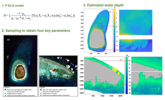
2. Dual-Band Log-Linear Analysis Model Based on Physics (P-DLA)

2.1. Formula Deduction

According to the single and quasi-single scattering theories and the single radiative transfer process in optically shallow water, the subsurface remote sensing reflectance ($r_{rs}$) can be expressed as follows [5,13,14]:

$$r_{rs}=r_{rs}^{dp}\left[1-exp\left(-gH\right)\right]+\frac{\rho }{\pi }exp\left(-gH\right)$$

(1)

where $r_{rs}^{dp}$ is the subsurface remote sensing reflectance in optical deep waters, $H$ is the water depth, and $\rho$ is the bottom reflectance modified by air-sea transmittance. Further, $g$ is the sum of the diffuse attenuation coefficients, which is approximated as $g=k_d+\left(k_u^C+k_u^B\right)/2$. Additionally, $k_d$ is the averaged diffuse attenuation coefficient of the perpendicular downwelling irradiance, $k_u^B$ is the averaged diffuse attenuation coefficient of perpendicular upwelling irradiance from sediments reflectance, and $k_u^C$ is the averaged diffuse attenuation coefficient of the averaged perpendicular upwelling irradiance from the water column.

A single-band log-linear model is obtained as follows by the logarithmic calculation and simplification of Equation (1) [15,16]:

$$X=\mathit{\text{-g}}H+ln{r}_b^{*}$$

(2)

where $X=ln\left(r_{rs}{\mathit{\text{-r}}}_{rs}^{dp}\right), ln\left(r_b^{*}\right)=ln\left(r_b{\mathrm{\text{-r}}}_{rs}^{dp}\right)$.

Considering that the blue and green bands are highly water permeable in visible light, these two bands are introduced into the model. The DLR model is conveyed as the following generalized vector equation [17]:

$$\stackrel{\rightharpoonup }{\alpha }\cdot \stackrel{\rightharpoonup }{X}=\stackrel{\rightharpoonup }{\alpha }\cdot {\stackrel{\rightharpoonup }{lnr}}_b-\left(\stackrel{\rightharpoonup }{\alpha }\cdot \stackrel{\rightharpoonup }{g}\right)H$$

(3)

where $\stackrel{\rightharpoonup }{X}=\left[X_1,X_2\right]$, $ln\left({\stackrel{\rightharpoonup }{r}}_b\right)=\left[ln{r}_{b1}^{*},ln{r}_{b2}^{*}\right]$, $\stackrel{\rightharpoonup }{g}=\left[g_1,g_2\right]$, $\stackrel{\rightharpoonup }{\alpha }=\left[{\alpha }_1,{\alpha }_2\right].$ These are the optimal band rotation coefficient unit vectors in the blue and green bands, and $\left|\stackrel{\rightharpoonup }{\alpha }\right|=1$. By analyzing the formula, the P-DLA model without the in-situ depth data is obtained as follows for the bathymetric estimation:

$$\left[{\alpha }_1,{\alpha }_2]\ast [X_1,X_2]=[{\alpha }_1,{\alpha }_2]\ast [{\mathrm{lnr}}_{b1}^{*},{\mathrm{lnr}}_{b2}^{*}\right]-\left\{\left[{\alpha }_1,{\alpha }_2]\ast [g_1,g_2\right]\right\}\ast H$$

(4)

$${\alpha }_1{\mathrm{lnr}}_{b1}^{*}+{\alpha }_2{\mathrm{lnr}}_{b2}^{*}=\left({\alpha }_1{\mathrm{lnr}}_{b1}^{*}+{\alpha }_2{\mathrm{lnr}}_{b2}^{*}\right)-\left({\alpha }_1{g}_1+{\alpha }_2{g}_2\right)\ast H$$

(5)

$$H=[\frac{-1/g_2}{g_1/g_2\ast {\alpha }_1+{\alpha }_2}]\ast [{\alpha }_1{X}_1+{\alpha }_2{X}_2-\left({\alpha }_1{\mathrm{lnr}}_{b1}^{*}+{\alpha }_2{\mathrm{lnr}}_{b2}^{*}\right)]$$

(6)

where (${\alpha }_1,{\alpha }_2$) is the weighted eigenvector of the blue and green bands, (${\alpha }_{1}ln\left(r_{b1}^{*}\right)+{\alpha }_{2}ln\left(r_{b2}^{*}\right)$) is the bottom parameters, ($g_1/g_2$) is the ratio of the attenuation coefficients in the blue and green bands, and ($g_2$) is the sum of the green band diffuse attenuation coefficients.

In the dual-band coordinate space, the optimal band rotation coefficient unit vector (${\alpha }_1,{\alpha }_2$) is linearly transformed for the spectral reflectance of the blue and green bands in the dataset ($X_1~X_2$), which are sampled for different types of sediments. This is done to obtain the new variable ($Y$), which is not affected by the change of the sediment type and has the greatest linear correlation with the water depth. Based on this, ${\alpha }_{1}ln\left(r_{b1}^{*}\right)+{\alpha }_{2}ln\left(r_{b2}^{*}\right)$ equals the origin parameter of $Y$ at a water depth of zero (on water boundaries). Finally, $Y$ is scaled to the water depth H through the parametric factor ($\frac{-1/g_2}{g_1/g_2\ast {\alpha }_1+{\alpha }_2}$), which is related to the inherent optical properties of $g_1/g_2$ and $g_2$ of the blue and green wavebands. Based on this, the shallow water depth is measured through all aforementioned parametric factors estimated by the multispectral remote sensing images.

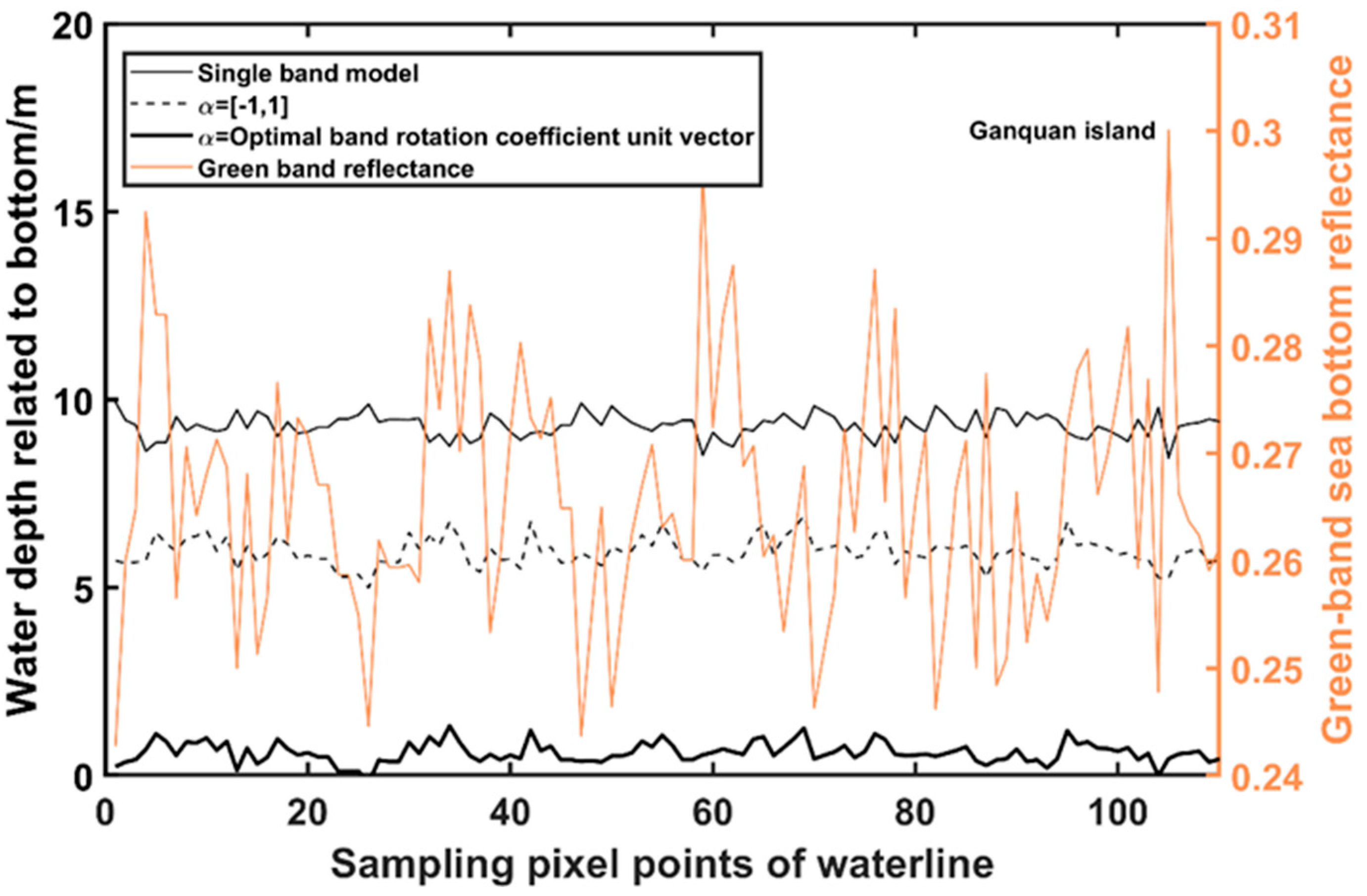
2.2. Optimal Band Rotation Coefficient Unit Vector

${\alpha }_1,{\alpha }_2$ are the weighted eigenvectors of the blue and green bands, and $Y$ is the scalar variable related to water depth. When the rotation coefficients of the two bands are optimal, the optimal band rotation coefficient unit vector ($\left[{\alpha }_1,{\alpha }_2\right]$) causes the $Y$-value to be linearly related to the water depth and unaffected by the change of the bottom sediment types. Assuming that water properties are spatially uniform, the optimal band rotation coefficient unit vector should be perpendicular to the line connecting all data points of the vector $X$ for all types of sediments at the same depth, which is analyzed from the perspective of geometric relationships [17]. Therefore, the estimation of the optimal band rotation coefficient of the unit vector with the pixels at the same depth of shallow water is a key step for the P-DLA model. Nonetheless, without relying on the prior data on the in-situ field measurements or laser radar detection, it is challenging to acquire spectral information about pixels at the same depth as the research regions. Regardless of the drastic changes in the submarine topography, when the spatial resolution of the multispectral remote sensing images is high enough (2 m in this paper), the water depth of the two adjacent pixels parallel with the coastlines may be deemed approximate. In the P-DLA model, a method based on adjacent pixel pairs is adopted. More specifically, a dataset of a group of adjacent pixel pairs ${(A,B)}_i$ is uniformly extracted at random from high-resolution remote sensing images of various sediments at different depths. By minimizing the adjacent pixel pairs ${(A,B)}_i$ corresponding to the optimal band rotation coefficient unit vector, the final optimal band rotation coefficient unit vector $\left[{\alpha }_1,{\alpha }_2\right]$ is calculated.

For any adjacent pixel pair ${(A,B)}_i$, the difference between $Y_A$ and $Y_B$ (defined as $\mathsf{\Delta }S{H}_i$) after applying the optimal band rotation coefficient unit vector, can be expressed as follows:

$$\Delta S{H}_i={\left|Y_A-Y_B\right|}_i$$

(7)

$$\Delta S{H}_i={\left|\left({\alpha }_1{X}_1^A+{\alpha }_2{X}_2^A\right)-\left({\alpha }_1{X}_1^B+{\alpha }_2{X}_2^B\right)\right|}_i$$

(8)

where $i$ is an adjacent pixel pair, and $A$ and $B$ correspond to two different types of sediments, respectively. After permutation, the formula is transformed as follows:

$$\Delta S{H}_i={\left|{\alpha }_1(X_1^A-X_1^B)+{\alpha }_2\left(X_2^A-X_2^B\right)\right|}_i$$

(9)

where $\mathsf{\Delta }S{H}_i$ is the $Y$-value pair of the optimal band rotation coefficient unit vector for the $X_1$ difference (conveyed as $\mathsf{\Delta }{X}_1$) and $X_2$ (conveyed as $\mathsf{\Delta }{X}_2$) difference in the spectral reflectance of the blue and green bands of any adjacent pixel pair.

Once the optimal band rotation coefficient unit vector is estimated, and the water depth is equal for each adjacent pixel pair, the differences in any $Y$-value pair and the sum of such differences are, theoretically, zero. However, under the actual conditions of the water environment, the water properties and reflectance of sediments exhibit variability that cannot be fully manually eliminated in adjacent pixel pairs of different spaces. The optimal band rotation coefficient unit vector cannot ensure that the sum of the differences in the $Y$-value pair of all sampled adjacent pixel pairs is zero. Therefore, the formula is solved as follows based on the minimum function ($argmin$):

$$f\left({\alpha }_1,{\alpha }_2\right)=argmin\left[{\displaystyle \sum }_{i=1}^n{(\mathsf{\Delta }S{H}_i)}^2\right]$$

(10)

where $f$ is the minimum function, n is the number of adjacent pixel pairs, and $\left|\stackrel{\rightharpoonup }{\alpha }\right|=1$. Notably, $\alpha =\left[-1,1\right]$ is the value when the blue and green bands are not rotated and do not represent the optimal solution.

2.3. Bottom Parameters

If $ln\left(r_b^{*}\right)$ of the two bands for a given sediment layer are known, ${\alpha }_{1}ln\left(r_{b1}^{*}\right)+{\alpha }_{2}ln\left(r_{b2}^{*}\right)$ is calculated based on the optimal band rotation coefficient unit vector ($\left[{\alpha }_1,{\alpha }_2\right]$). Nonetheless, there are multiple types of sediments mixed in actual water environments. Minor differences generally exist in albedo among different types of sediments and cannot be fully eliminated. Hence, in actual calculations, the albedo of the different sediments should be fully considered and used.

In general, there are one or more types of sediments, such as coral reefs, coral reef sand, algae, and other sediments that the naked eye cannot recognize on the waterline. These sediments are the same as those mixed in shallow water areas. Suppose the spatial resolution of remote sensing images is quite high (2 m for the $WorldView-2$ remote sensing images used in this paper). In that case, the water depth should be approximately zero for most pixels near the instantaneous coastlines [18]. Assuming that the water depth on the waterline is zero, then ${\alpha }_1{X}_1+{\alpha }_2{X}_2$ may be approximated as ${\alpha }_{1}ln\left(r_{b1}^{*}\right)+{\alpha }_{2}ln\left(r_{b2}^{*}\right)$. As mentioned above, when $\left[{\alpha }_1,{\alpha }_2\right]$ is optimal, ${\alpha }_1{X}_1+{\alpha }_2{X}_2$ is approximate among different types of sediments. Therefore, in this paper, a certain number of pixels from various sediments are sampled near the waterline, and data on the reflectance of sediments is extracted. From this, the sediment parameters of the research regions are calculated based on the mean ${\alpha }_{1}ln\left(r_{b1}^{*}\right)+{\alpha }_{2}ln\left(r_{b2}^{*}\right)$ of various sediments. In the near-infrared bands, the images of the water bodies appear black since the water is highly absorptive. Therefore, the waterline is directly recognized through near-infrared images.

Pixels were gathered from different types of sediments near the waterline of Ganquan Island. Further, the relationship between the sediment parameters and the sediment-related reference water depth obtained by three different methods was calculated. The three methods used are (i) the single-band water depth inversion model (see Formula (2)), (ii) the dual-band log-linear analysis model when $\alpha =\left[-1,1\right]$, and (iii) the dual-band log-linear analysis model when $\alpha$ is the optimal band rotation coefficient unit vector. Meanwhile, the reflectance of the green band is shown in Figure 1. Figure 1 shows that the change of water depth caused by different sediments was less than that of the other two methods when $\alpha$ is optimal. Furthermore, the computed reference water depth related to the bottom is generally 0–1 m. This indicates that the estimation of the bottom parameters via the waterline significantly alleviates the effects of the changes in the type of sediments upon the water depth.

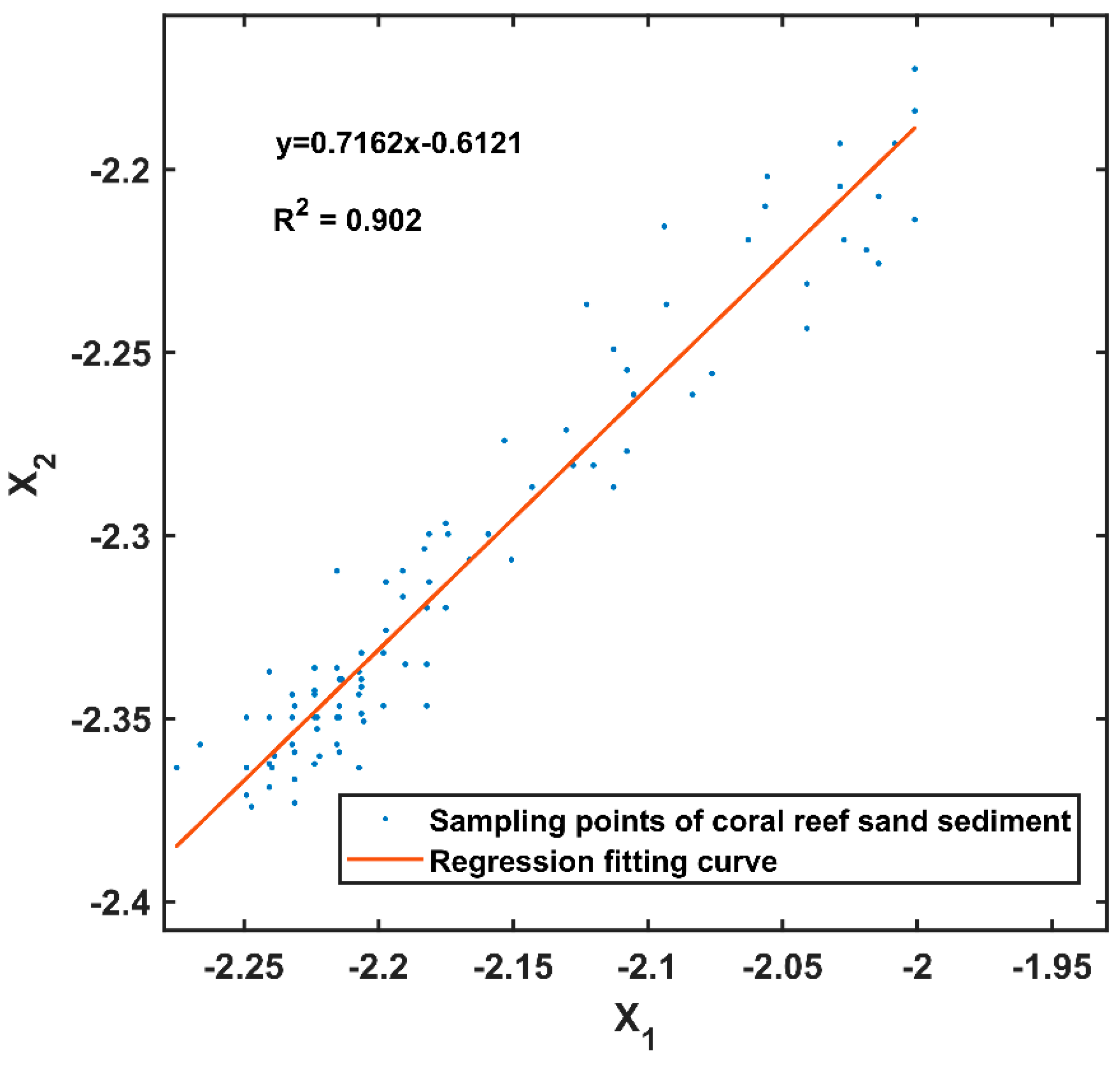
2.4. Ratio between Diffuse Attenuation Coefficients of the Blue and Green Bands

$g_1/g_2$ can be obtained from the linear regression equation constructed by the $X_1~X_2$ dataset. The following formula can be deduced by applying Formula (2) to the blue and green bands of remote sensing images, respectively, and eliminating the water depth variable ($H$):

$$X_1=\left(g_1/g_2\right)\ast X_2+\left(ln{r}_{b1}^{*}-\left(g_1/g_2\right)\ast ln{r}_{b2}^{*}\right)$$

(11)

$$X_1=\left(g_1/g_2\right)\ast X_2+\beta$$

(12)

where $ln{r}_{b1}^{*}-\left(g_1/g_2\right)\ast ln{r}_{b2}^{*}$ is the characteristic exponent of the sediment type (defined as $\beta$), which varies among the different types of sediments:

$$\beta =ln{r}_{b1}^{*}-\left(g_1/g_2\right)\ast ln{r}_{b2}^{*}$$

(13)

Assuming that shallow water properties are uniform in nature, the ratio of the attenuation coefficients between the blue and green bands is conveyed as $g_1/g_2$ and remains spatially unchanged. Therefore, $g_1/g_2$ is deemed as the slope of the regression equation established with the dataset $X_1~X_2$. By collecting the dataset, $X_1~X_2$ on the same type of submarine sediments at varying water depths (coral reef sand) from multispectral remote sensing images with high spatial resolution, a unitary linear regression equation is created. Specifically, the ratio of the attenuation coefficients between the blue and green bands ($g_1/g_2$) is determined, as shown in Figure 2. The determination coefficient ($R^2$) of the fitting equation is 0.902, close to 1. Therefore, it is well-fitted. It is reasonable to assume that the shallow water properties are uniform in this method. However, the water body itself is still affected by chlorophyll-a, suspended solids, and bottom sediments.

2.5. Diffuse Attenuation Coefficients of the Green Band Estimated by QAA

$QAA$ (quasi-analytical algorithm [QAA]) was proposed and constantly updated by Lee et al. [19]. Based on the radiative transfer principles, it can determine the absorption coefficient ($a$), backscattering coefficient ($b_b$), and other inherent optical properties of water. This is done by analyzing data on remote sensing reflectance and inverting the corresponding water quality parameters depending on the inherent optical properties of water [10,19,20,21,22,23,24,25]. From the above, it is known that $g_2=k_d+(k_u^B+k_U^C)/2$, where $k_d$, $k_u^B$, and $k_u^C$ are closely related to the solar zenith angle, the satellite zenith angle, and the inherent optical properties (IOPs) of seawater. This is especially true for the absorption coefficient ($a$) and the backscattering coefficient ($b_b$) [6,25]. In this paper, QAA_v6, the latest version of $QAA$ is used [26], and its calculation process is as follows:

$$r_{rs}^{dp}\left(\lambda \right)=\left[p_0+p_{1}u\right]u\left(\lambda \right)$$

(14)

$$u\left(\lambda \right)=\frac{-p_0+\sqrt{{(p_0)}^2+4p_1\ast r_{rs}^{dp}\left(\lambda \right)}}{2p_1}$$

(15)

$$r_{rs}\left(\lambda \right)=\frac{R_{rs}\left(\lambda \right)}{0.52+1.7R_{rs}\left(\lambda \right)}$$

(16)

$$u=b_b/\left(a+b_b\right)$$

(17)

where $R_{rs}$ is the remote sensing reflectance of the surface water received by the satellite sensor, $\lambda$ is the representative wavelength of the images, $u$ is a $G\mathrm{or}don$ parameter [27], and $p_0$ and $p_1$ are constants of the water model. These are taken as $0.0895$ and $0.1247$, respectively, in type I marine water in high scattering regions [19].

The absorption coefficient of the green band of multispectral remote sensing images ($a_{green}$) is calculated using the $QAA-555$ algorithm, as shown in Equation (16) [19,25], where the central wavelength of the red and green bands are 640 nm and 555 nm, respectively.

$$a_{green}=a_w^{green}+0.56\left\{{\left[\frac{r_{rs\_red}^{dp}}{r_{rs\_green}^{dp}}\right]}^{1.7}-0.03\right\}$$

(18)

where $r_{rs\_\mathrm{green}}^{dp}$ and $r_{rs\_red}^{dp}$ are the optical deep subsurface remote sensing reflectance’s of the green and red bands, respectively, and $a_w^{green}$ is the averaged pure water absorption coefficient of the green band [25].

$$A_w^{green}=\frac{{{\displaystyle \int }}_{{\lambda }_1}^{{\lambda }_2}RS{R}_i\left(1/a_w\left(\lambda \right)\right)d\lambda }{{{\displaystyle \int }}_{{\lambda }_1}^{{\lambda }_2}RS{R}_i\left(\lambda \right)d\lambda }$$

(19)

$$a_w^{green}=1/A_w^{green}$$

(20)

where ${\lambda }_1$ and ${\lambda }_2$ are the spectral wavelength ranges of the green and red bands of the satellite images, $RS{R}_i\left(\lambda \right)$ is the spectral response function of a certain band, and $a_w\left(\lambda \right)$ is the average absorption coefficient of the pure water at a certain wavelength [28].

If $a_{green}$ is known, $b_b^{green}$ is calculated as follows:

$$b_b^{green}=\frac{u_{green}\ast a_{green}}{1-u_{green}}$$

(21)

Once $a_{green}$ and $b_b^{green}$ are known, $k_d$ is determined as follows:

$$k_d=\left(1+m_0\ast {\theta }_s\right)a_{green}+\left(1-\gamma \frac{b_{bw}^{green}}{b_b^{green}}\right)\ast m_1\ast \left(1-m_2{e}^{-m_3\ast a_{green}}\right)b_b^{green}$$

(22)

$$b_{bw}^{green}=\frac{{{\displaystyle \int }}_{{\lambda }_1}^{{\lambda }_2}RS{R}_i\left(\lambda \right)b_{bw}\left(\lambda \right)d\lambda }{{{\displaystyle \int }}_{{\lambda }_1}^{{\lambda }_2}RS{R}_i\left(\lambda \right)d\lambda }$$

(23)

$$b_{bw}\left(\lambda \right)=0.00144{(\lambda /500)}^{-4.32}$$

(24)

where $m_0-m_3$ and $\gamma$ are model constants independent of different properties and the spectral wavelength of the water column. These are taken as 0.005, 4.26, 0.52, 10.8, and 0.265, respectively [25]. Further, ${\theta }_s$ is the solar zenith angle, and $b_{bw}\left(\lambda \right)$ is the backscattering coefficient of the pure water at a certain wavelength.

$$k_u^C=\frac{1}{\cos ({\theta }_v)}\left(a_{green}+b_b^{green}\right)\ast D_u^C$$

(25)

$$D_u^C=1.03{(1+2.4u)}^{0.5}$$

(26)

$$k_u^B=\frac{1}{\cos ({\theta }_v)}\left(a_{green}+b_b^{green}\right)\ast D_u^B$$

(27)

$$D_u^B=1.04{(1+5.4u)}^{0.5}$$

(28)

$$g_2=k_d+\left(k_u^B+k_u^C\right)/2$$

(29)

where ${\theta }_v$ is the satellite zenith angle, $D_u^C$ and $D_u^B$ are the optical amplification coefficients of the increased scattering from the water column and water bottom, respectively. When $u$ is less than 0.6, $D_u^C$ and $D_u^B$ are generally in the range of 1.2–1.7 and 1.1–2.2, respectively [5,29].

3. Study Areas and Data Processing

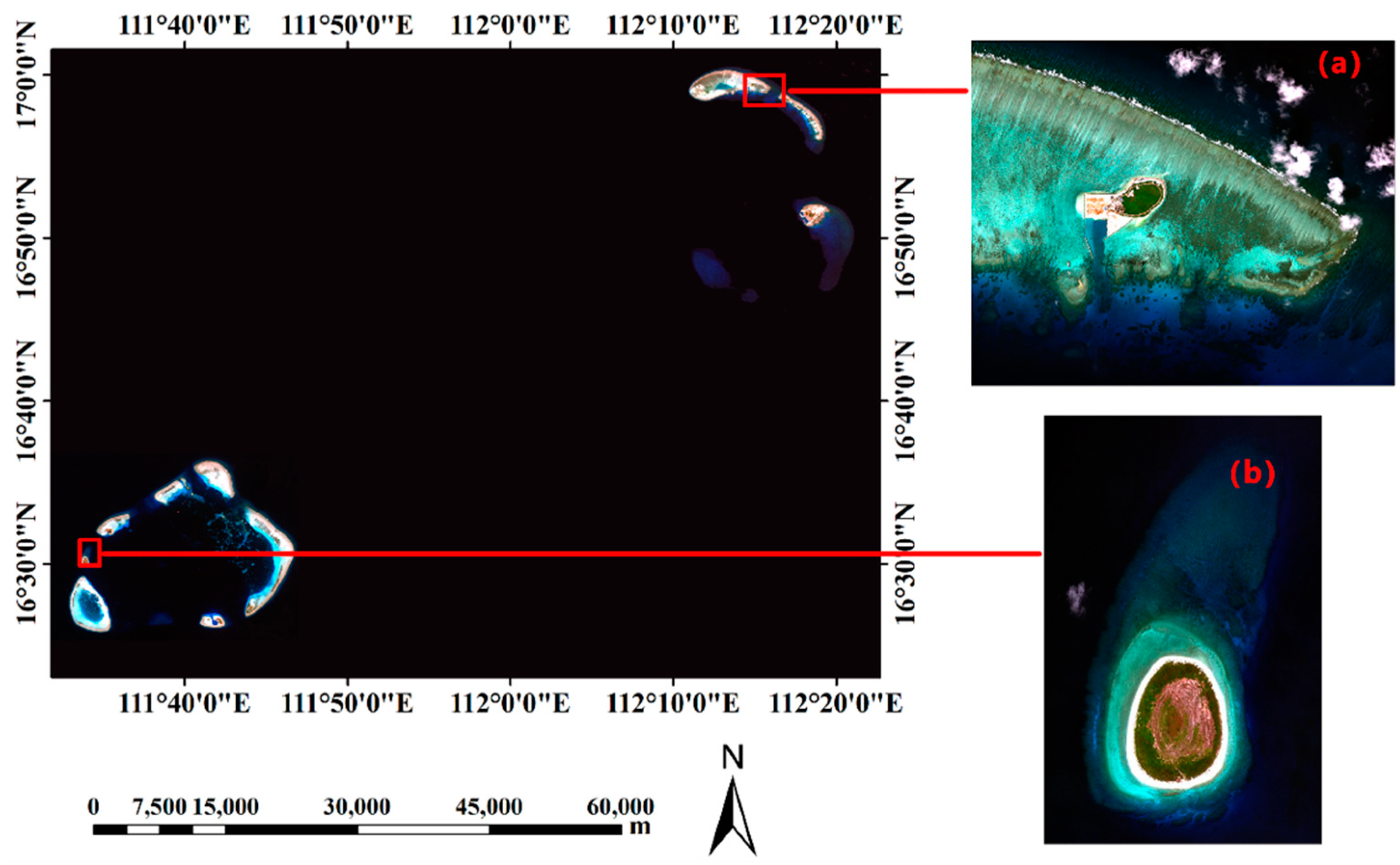
3.1. The Study Areas and Datasets

The shallow water (0–20 m) around Ganquan Island and Zhaoshu Island in the South China Sea is used for the bathymetry experiment, which belongs to Case I marine water (Figure 3). Ganquan Island is located in Yongle Atoll of the Xisha Islands, with a central longitude and latitude of $\left(16°30\prime \hspace{0.17em}\mathrm{N},\hspace{0.17em}111°35\prime \hspace{0.17em}\mathrm{E}\right)$. The terrestrial area of the Ganquan Island is oval, where the pilot zone is approximately 2 km long from the north to the south and nearly 1 km wide from the east to the west. This terrestrial area is composed of land with an approximate area of 0.6 km², and the waters nearly cover an area of 1.1 km². The mean water depth is 8.9 m, and the water depth changes slowly and relatively hierarchically.

Zhaoshu Island is north of Qilian Island in the Xuande Islands at a central longitude and latitude of $\left(16°59\prime \hspace{0.17em}\mathrm{N},\hspace{0.17em}112°16\prime \hspace{0.17em}\mathrm{E}\right)$. It extends from the northwest to the southeast, including land that approximately covers an area of 6.7 km² and pilot waters with an area of 5.6 km². In this area, the mean water depth is 7.5 m. Spurs and grooves are widely distributed on reef slopes northeast and west of the island. The variations in the water depth are drastic, somewhat impacting the precision of the water depth inversion.

The water is limpid in both research regions, where the underwater sediments are mainly coral reef sand, coral reefs, algae, and so on [3,30,31]. With striking differences in the water depth, they have visibly limpid shallow sea areas and deep-water areas, where the bottom cannot be seen. These water bodies are suitable for conducting multispectral remote sensing water depth inversion.

All satellite remote sensing images in these two study areas are collected from the $WorldView-2$ standard multispectral images of four bands (blue, green, red, and near-infrared 1), with a spatial resolution of 2 m. The spectral bandwidth ranges are as follows: 450–510 nm in the blue band, 510–580 nm in the green band, 630–690 nm in the red band, and 770–895 nm in the near-infrared 1 band. The $WorldView-2$ satellite remote sensing images of Ganquan Island and Zhaoshu Island were generated on 2 April 2014, and 11 March 2017, respectively (

Table 1. Parameter information of WorldView-2 images in two regions.

Research Regions	Acquisition Date	Cloud Fraction	Solar Zenith Angle	Satellite Zenith Angle	Tidal Height/m
Ganquan Island	2 April 2014	0.1%	19.4°	36.3°	0.78
Zhaoshu Island	11 March 2017	0.6%	31.6°	27.6°	0.21

). Two remote sensing images are pre-processed by radiometric calibration, atmospheric correction, geometric correction, and land-water separation. Among them, radiation calibration converts dimensionless digital values in remote sensing images into relative physical values (apparent radiance).

$$L_{\lambda }=\frac{DN\ast absCalFactor}{effectiveBandwidth}$$

(30)

where, $L_{\lambda }$ is the radiance value received by the sensor, and the unit is $W/\left({\mathrm{m}}^2\cdot \mathsf{\mu }\mathrm{m}\cdot \mathrm{sr}\right)$. Further, $absCalFactor$ is the absolute scaling factor, and the unit of $effectiveBandwidth$ is in μm. The metadata information is stored in the *.IMD file.

In the study of ocean optical remote sensing, only about 10% of the energy received by satellite sensors is radiated from the water body. Therefore, it is necessary to carry out the atmospheric correction to remove the scattering and reflection effects from atmospheric molecules and aerosols [30,32,33]. The FLAASH atmospheric correction model developed by the Air Force Research Laboratory, Hanscom AFB, and Spectral Sciences, Inc. is based on the MODTRAN (MODerate resolution atmospheric TRANsmission) [34]. In this paper, the FLAASH module integrated into the environment for visualizing images (ENVI) was used for atmospheric correction of the images. For Zhaoshu Island, the cloud fraction of $WorldView-2$ images was 0.6%. Some cloud-containing areas of Zhaoshu Island were masked to reduce the impacts of cloud-borne areas upon the precision of this experiment.

The ground truth depth data was selected to evaluate the precision of the water depth estimation results for the research regions to quantitatively evaluate the effectiveness of this bathymetric inversion algorithm without in-situ depth data (Figure 4). The data on the in-situ depths of Ganquan Island was acquired on 9 January 2013, from the lidar point cloud data gathered by the $SHOAL-3000$ airborne lidar bathymetry system of the Optech firm. The horizontal precision of lidar depths was 2.5 m, and the bathymetric precision was 0.15 m. The in-situ depth data of Zhaoshu Island was acquired on 2 March 2014 by a Chinese research institute in combination with single-beam and manual measurements. The overall bathymetric precision was better than 1% of the water depth (

Table 2. Information on the actual water depth of the two research regions.

Research Regions	Data Source	Acquisition Date	Data Precision	Number of Points with In-Situ Depth Data	Mean Water Depth
Ganquan Island	$SHOAL-3000$ Airborne Lidar detection system	9 January 2013	0.15 m	437	−8.95 m
Zhaoshu Island	Combination of single-beam and manual measurements	2 March 2014	1% above the Precision of Water Depth	1900	−7.45 m

). This paper’s in-situ water depth data is the steady-state water depth based on the theoretical depth datum. Meanwhile, the water depth ($H$) extracted by the bathymetric inversion model was the instantaneous depth of the sea level calculated at the time of the image transit. Thus, the tidal correction was completed with the following formula:

$$H=Z-tide$$

(31)

where $H$ is the instantaneous water depth of the images when the remote satellite transits, $Z$ is the seawater depth measured under the steady-state, and $tide$ is the instantaneous tidal level measured when the satellite transits. The global tidal model was used to obtain the tidal values in the study areas.

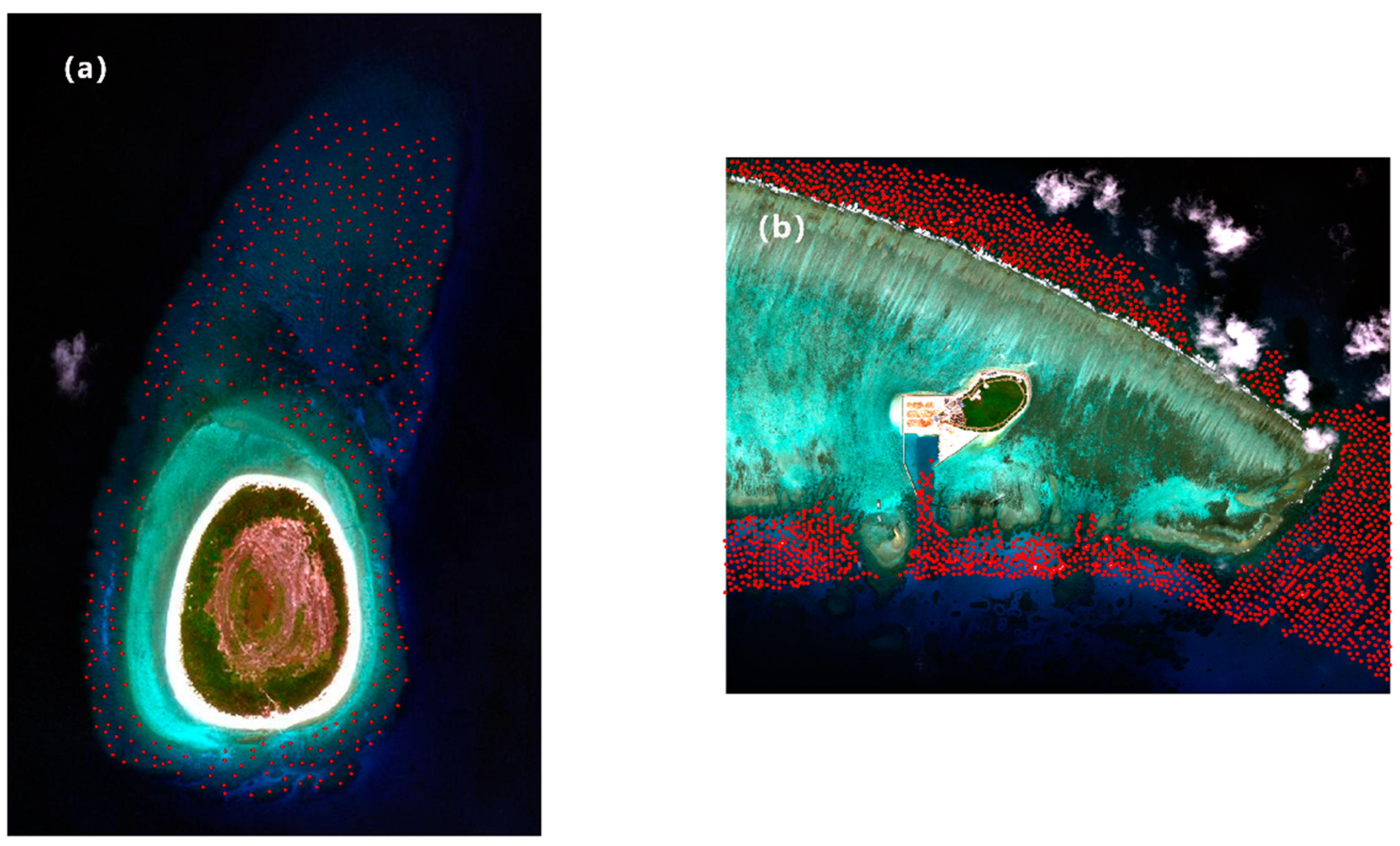
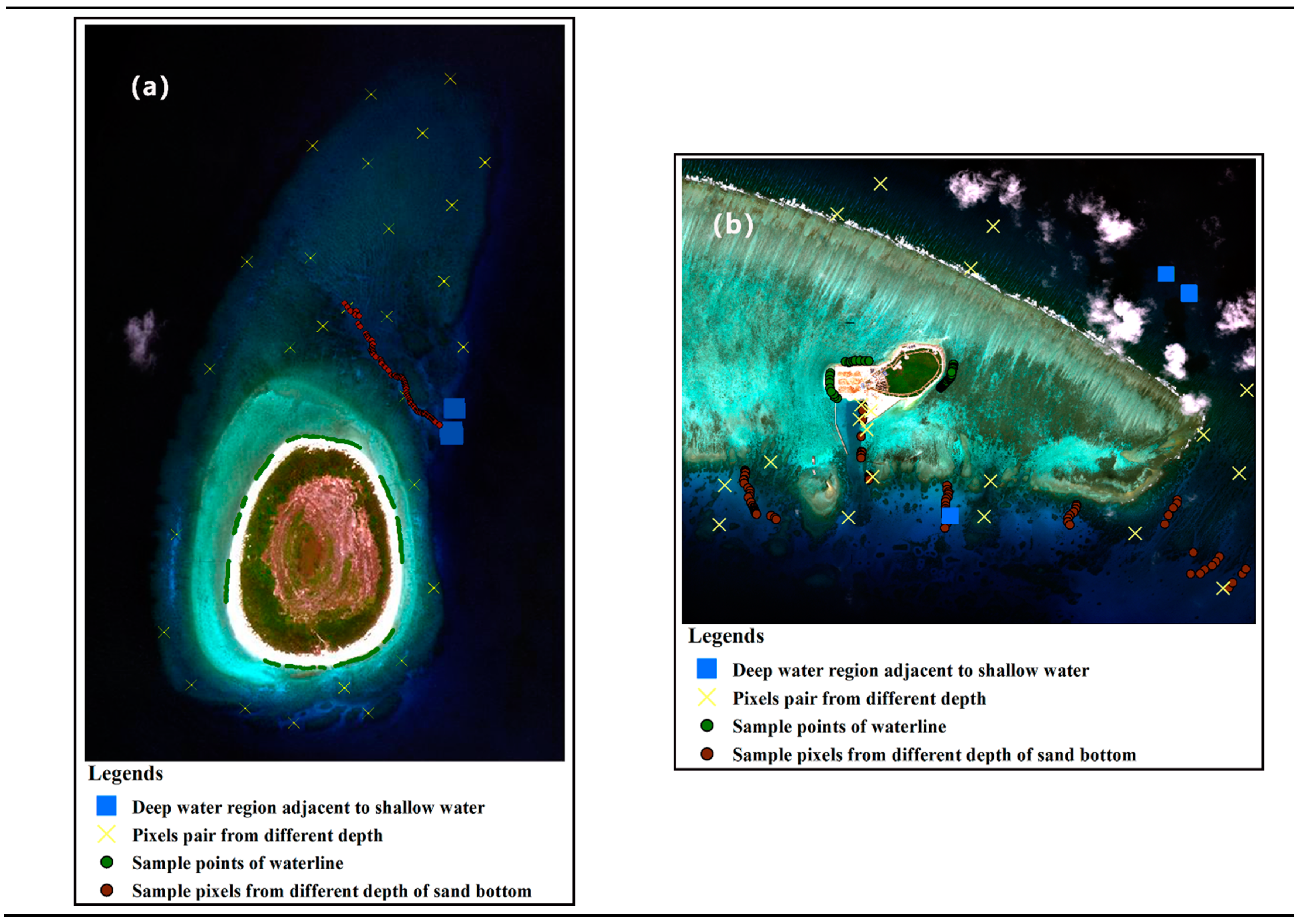
3.2. Collection of Sample Pixels

After the pre-processing of the $WorldView-2$ images, four different types of sample pixels were collected from the two regions, and the spectral information on the remote sensing reflectance of each sample was directly extracted. The four types of sample pixels correspond to the unknown parameters of the P-DLA model without in-situ depth data. This includes adjacent pixel pairs with different depths, typical sediment pixels near the waterline, pixels of the same sediment from different water depths (sandy sediments are adopted in this paper), and the deep-water pixels of adjacent shallow water areas. The specific distribution of the sampling points is shown in Figure 5.

3.3. Evaluation

Multiple types of indicators for the evaluation can quantitatively evaluate the bathymetric estimation results of the P-DLA model without in-situ depth data. In this paper, the root mean square error ($RMSE$), the mean absolute error ($MAE$), the mean relative error ($MRE$), and the correlation coefficient ($r$) were used as the main indicators for the evaluation. $RMSE$ and $MRE$ are expressed as follows:

$$RMSE=\sqrt{\frac{{{\displaystyle \sum }}_{i=1}^n{(x_i-y_i)}^2}{n}}$$

(32)

$$MRE=\frac{1}{n}{\displaystyle \sum }_{i=1}^n\frac{\left|x_i-y_i\right|}{y_i}$$

(33)

4. Results

4.1. Estimated Parameters

First, the spectral information on the geographic coordinates and pixels is extracted from different sampling points. Next, the parameters necessary for the model are respectively calculated according to the above formulas (

Table 3. Estimated Parameters of Two Regions.

	${\mathit{\alpha }}_1$	${\mathit{\alpha }}_2$	${\mathit{\alpha }}_1\mathbf{ln}{\mathit{r}}_{\mathit{b}1}^{*}+{\mathit{\alpha }}_2\mathbf{ln}{\mathit{r}}_{\mathit{b}2}^{*}$	${\mathit{g}}_1/{\mathit{g}}_2$	${\mathit{g}}_2$
Ganquan Island	−0.755	0.655	0.329	0.716	0.143
Zhaoshu Island	−0.674	0.738	−0.043	0.894	0.178

). Finally, the model-determined parameters are applied in the formulas to estimate the water depth of the whole remote sensing image by inversion.

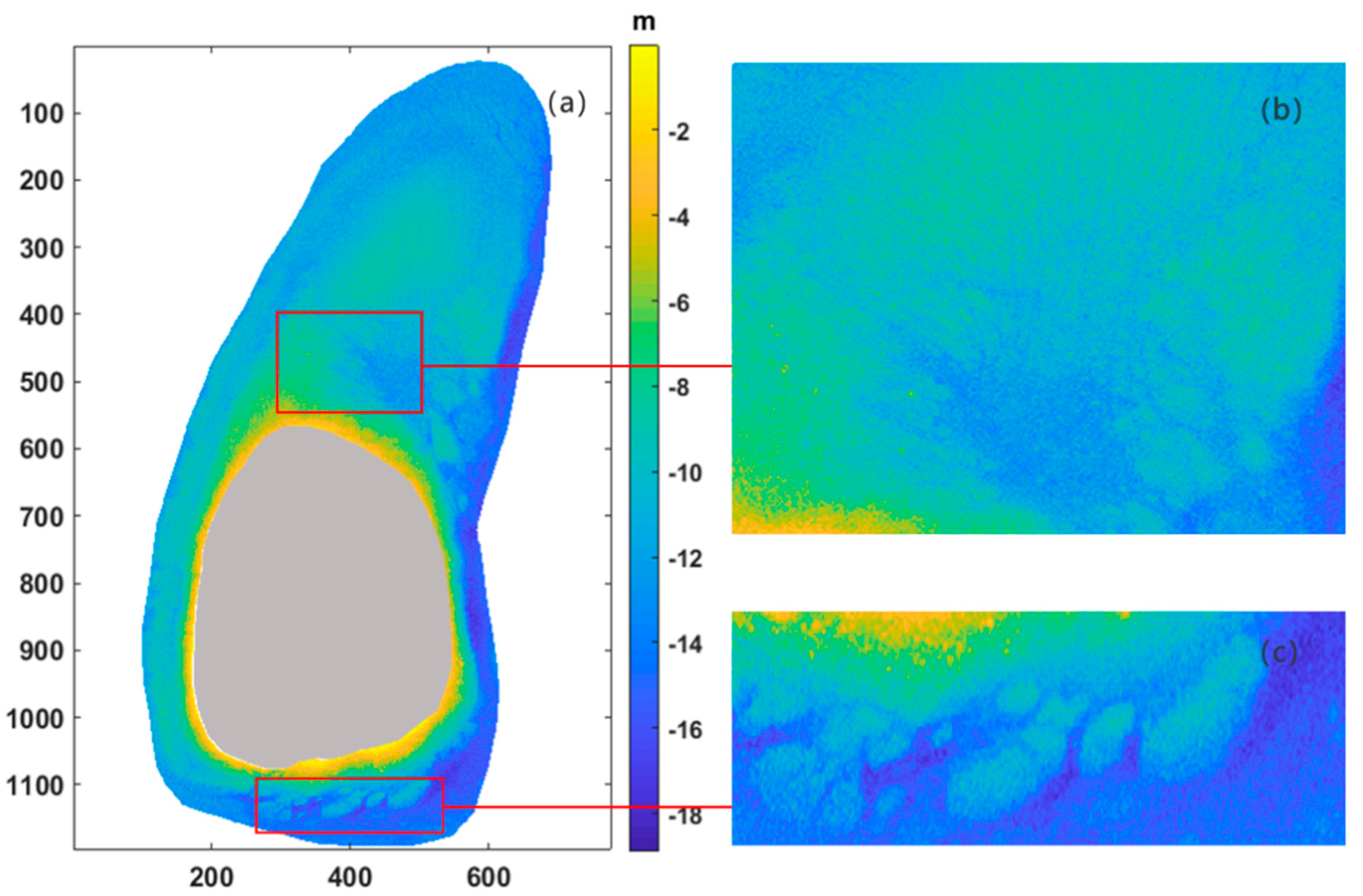
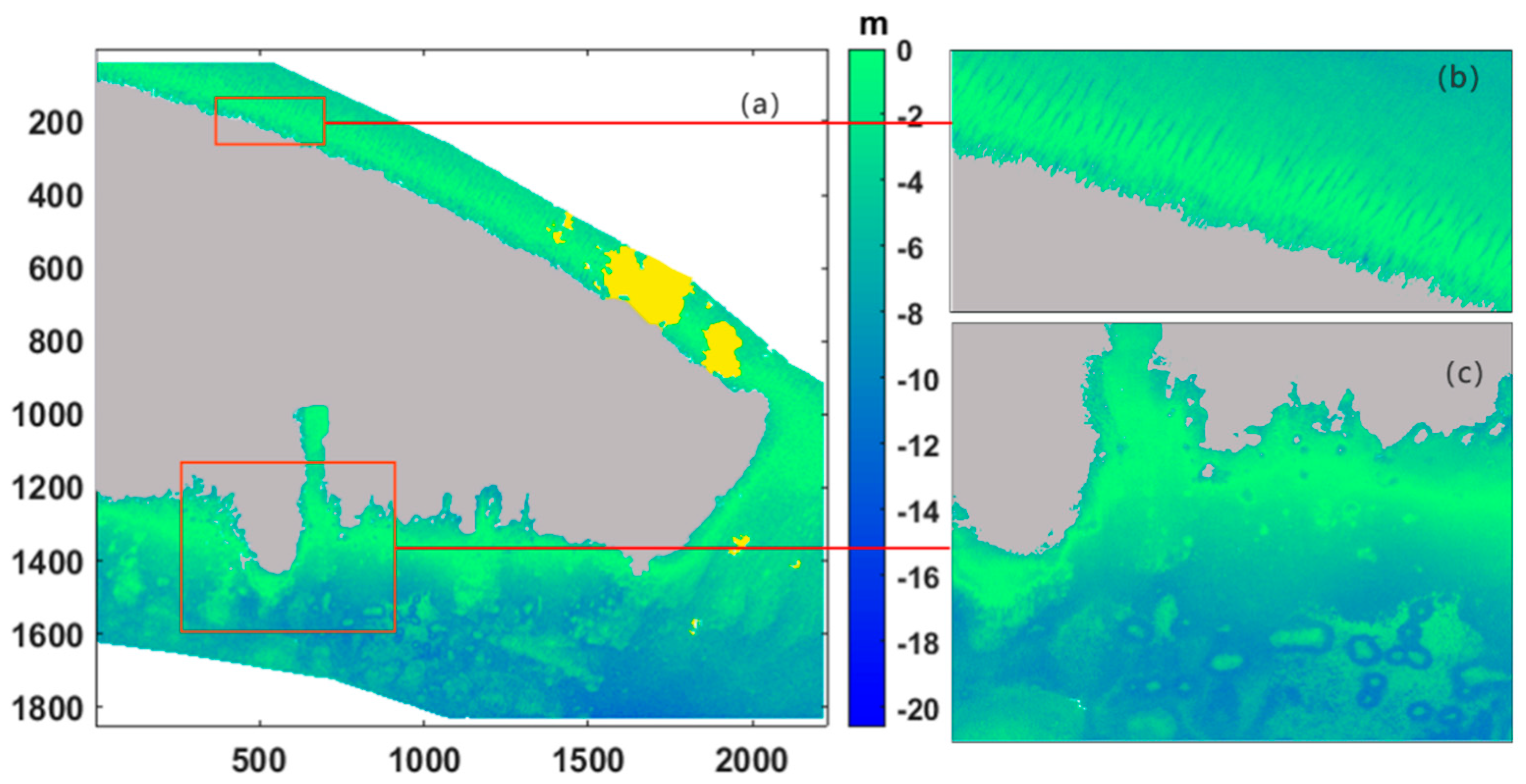
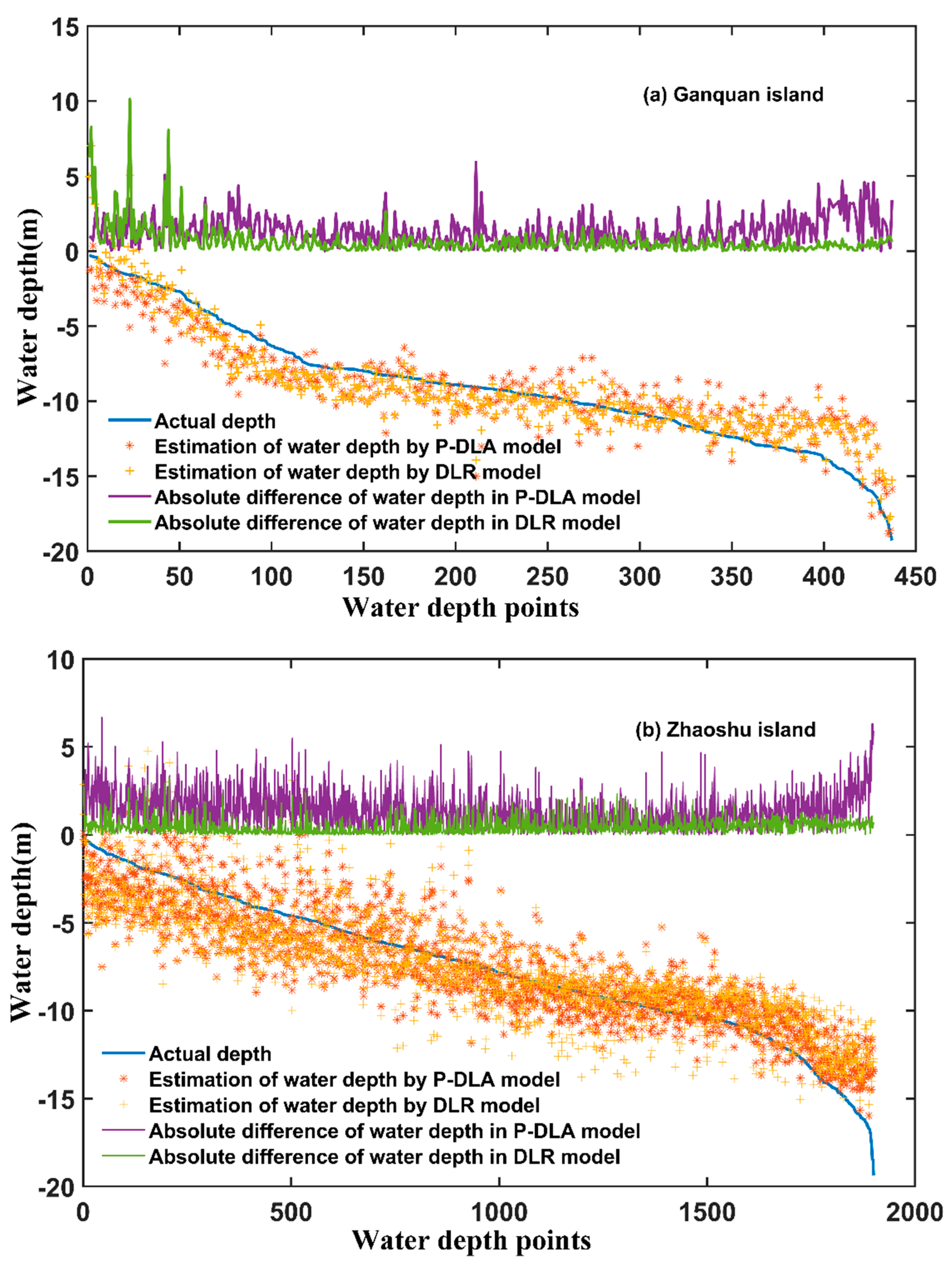
4.2. Bathymetric Estimated Results

The bathymetric results estimated by the P-DLA model without in-situ depth data are shown in Figure 6 and Figure 7, respectively. As shown, the grey zone in the middle denotes the land above sea level. The peripheral white zone is the deep-water optical zone to which bathymetric inversion does not apply. Further, the yellow zone of Zhaoshu Island is shrouded with a thin cloud. The P-DLA model estimates the underwater depth pixel by pixel. Therefore, the resolution of the digital elevation model (DEM) and remote sensing images from the inversion results are the same height of 2 m. Figure 6 and Figure 7’s inversion results show that the water depth ranged from 0–20 m, and the water depth variation trend is consistent with the actual water depth materials and previous literature [3,8]. From the local details of the figures, this method inverts detailed underwater topographic features of Ganquan Island and Zhaoshu Island. An example is the bathymetric estimated results of the northwest reef front slope of Zhaoshu Island (Figure 7b). The landform of the underwater reef ridge trough in the northeast-southwest direction is displayed. Because these slopes are windward, where the oxygen content is high in the seawater, coral reefs grow relatively well, and spurs and grooves arise from perennial seawater erosion.

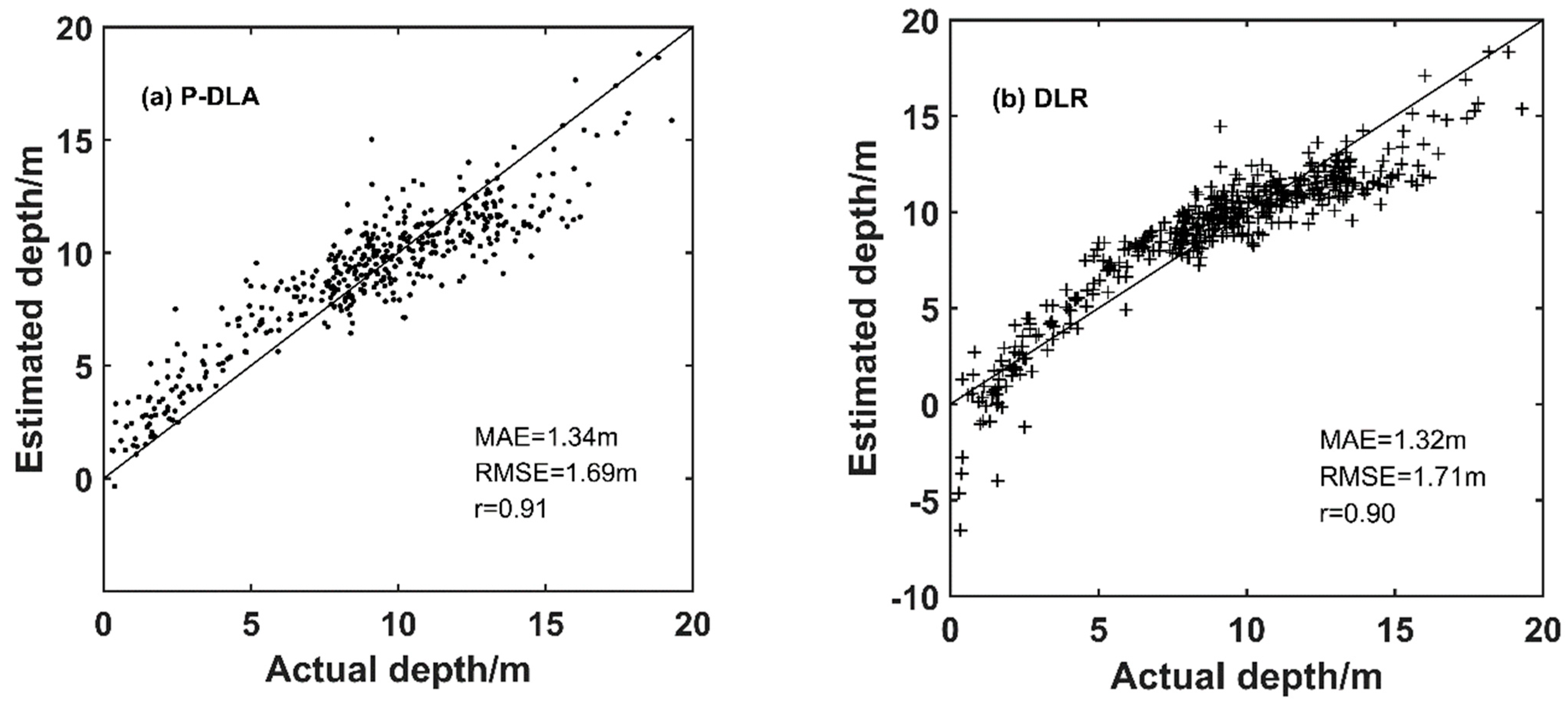
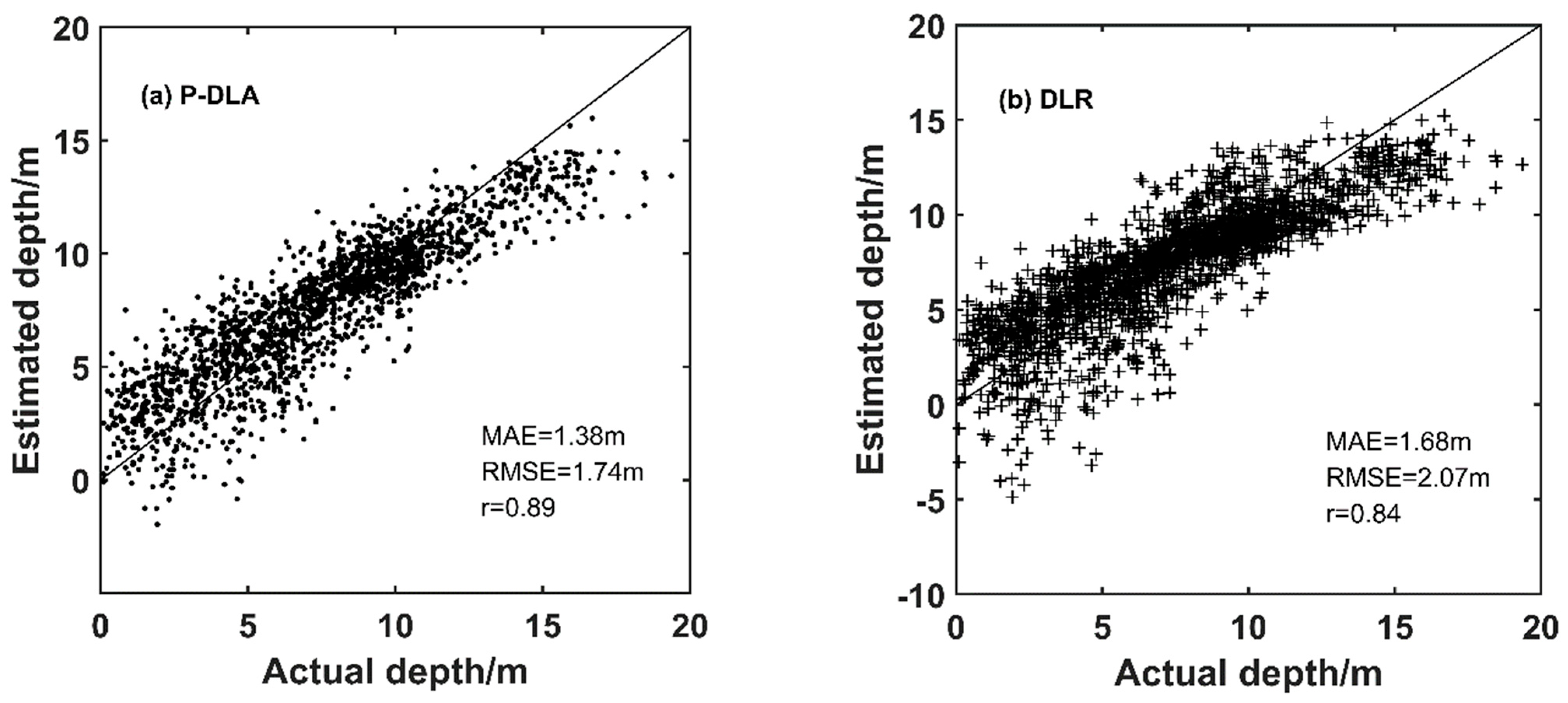
4.3. Accuracy Evaluation

The mean absolute error, mean relative error, root mean square error, and correlation coefficient between the water depth of the two research regions measured by the P-DLA model and the actual water depth were calculated. Related indicators for evaluation are listed in

Table 4. Precision evaluation for the overall water depth estimation.

	RMSE/m	MAE/m	MRE	r
Ganquan Island	1.692	1.348	0.148	0.914
Zhaoshu Island	1.744	1.385	0.183	0.895

. For Ganquan Island and Zhaoshu Island, the $RMSE$ values were 1.69 m and 1.74 m, the $MRE$ values were 14.8% and 18.3%, and the r values were 0.914 and 0.895, respectively. This demonstrates that using the P-DLA model for bathymetry can produce a reasonable estimation of shallow water depth. However, the overall bathymetric results of Ganquan Island outperform those of Zhaoshu Island due to its steadier changes in submarine sediments. Furthermore, there is less in-situ depth data for the precision validation in Ganquan Island than in Zhaoshu Island.

This paper measured water depth every 5 m and obtained the precision evaluation results of four different water depth ranges to better evaluate the bathymetric estimation results of the two regions obtained from the P-DLA model. As shown in

Table 5. Precision evaluation for varying water depths.

Research Regions	Indicators for Evaluation	0–5 m	5–10 m	10–15 m	15–20 m
Ganquan Island	RMSE/m	1.805	1.456	1.708	2.674
	MAE/m	1.493	1.165	1.362	2.238
	MRE	0.375	0.129	0.123	0.154
Zhaoshu Island	RMSE/m	2.084	1.416	1.477	3.230
	MAE/m	1.755	1.098	1.204	2.962
	MRE	0.426	0.141	0.113	0.225

, the $RMSE$ was close to 2 m, and the $MRE$ was about 40% at water depths between 0 m and 5 m for both islands. In these areas, the inversion precision was relatively poor. This can be explained by the multiple types of sediments being mixed in the near-coastal areas of the two regions. Consequently, the water properties change significantly, the sea surface is easily affected by the scattering of natural phenomena (e.g., beachcomber, whitecap), and the apparent optical properties change significantly. At the water depth of the two regions ranging from 5–15 m, the RMSE was better than 1.5 m, and the $MRE$ was below 15%. The inversion precision of the model was high. At the water depths ranging between 15 m and 20 m, the $RMSE$ was 2.67 m and 3.23 m, and the $MRE$ was 15.4% and 22.5% for Ganquan Island and Zhaoshu Island, respectively. The $RMSE$ and $MRE$ increased in the shallow seawater depth, demonstrating that this model exhibits weaker inversion capacity in optically deep-water zones.

5. Discussion

5.1. Comparison of Water Depth Inversion with and without In-Situ Depth Data

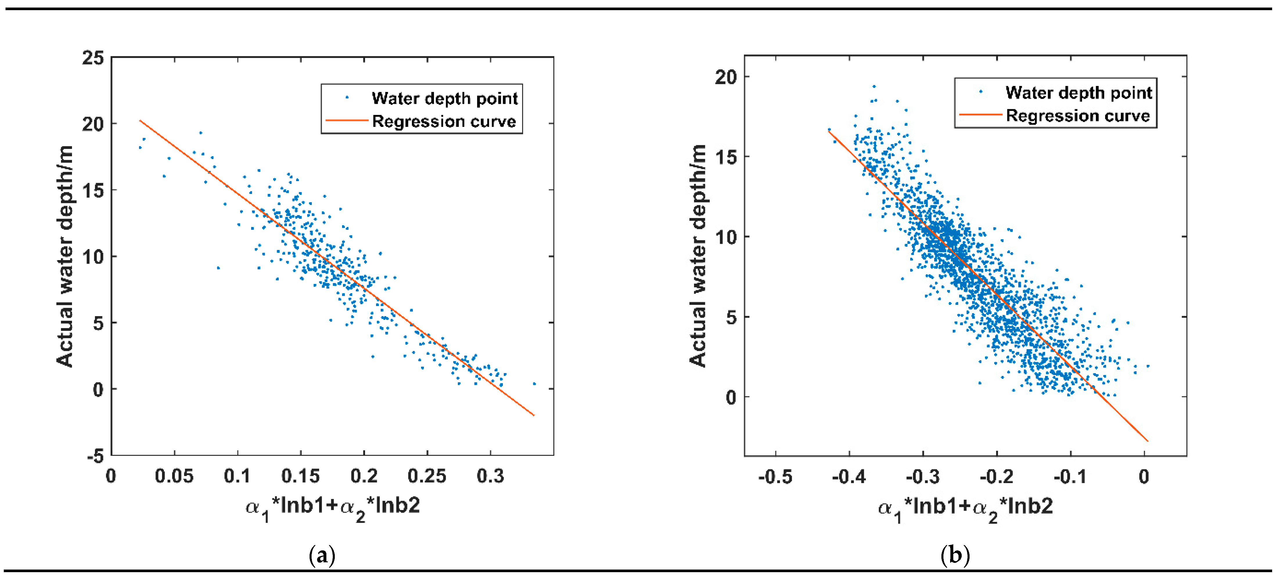
The DLR model is a common semi-theoretical and semi-empirical bathymetric inversion model. It solves unknown parameters based on in-situ depth data and band reflectivity for passive optical remote sensing bathymetric inversion. The applicability and inversion precision of this model have been fully studied and verified. According to previous research findings, under different water qualities and bottom conditions, the overall $RMSE$ and $MRE$ of the bathymetric inversion using the DLR model were 1–3 m and 15–30%, respectively [30,35,36,37]. In this experiment, the in-situ bathymetric samples of the two regions were divided into training and validation samples at a ratio of 7:3. From them, the training samples were used to establish linear model relationships between the multi-band reflectivity of multispectral remote sensing images and in-situ depth data. The validation samples were utilized to evaluate the precision of the linear water inversion model. For details of the DLR model, refer to

Table 6. Information of the DLR model.

Research Regions	Number of Training Samples	Number of Validation Samples	Bathymetric Inversion Model	r
Ganquan Island	305	132	−10.84 + 366.53 * log(B1) + 410.87 * log(B2)	0.900
Zhaoshu Island	1330	570	−8.9 + (−276.18) * log(B1) + (322.21) * log(B2)	0.843

. In the formula, B1 represents the blue band. Meanwhile, B2 denotes the green band.

Figure 8 and Figure 9 show the scatter plots of the actual and estimated depth on Ganquan Island and Zhaoshu Island. The closer the scatter points of water depth are to the 1:1 standard line, the smaller the deviation between the estimated and actual water depth at each validation point, and the higher the inversion precision. For the two regions, the bathymetric results and scatter plots of the P-DLA model, and the DLR model are similar. Both models cohere well with the 1:1 standard line, with their $RMSE$ values within 1.5–2 m, and their bathymetry precisions were comparable. In estimating the water depth of Ganquan Island with the P-DLA model, the $RMSE$ was 1.69 m, and the r was 0.91, which are 1.3% and 1.5% higher than those of the DLR model. The bathymetric estimation of Zhaoshu Island by the P-DLA model suggests that the RMSE was 1.74 m and the r was 0.89, which are 18.9% and 5.8% higher than those of DLR. This demonstrates that the P-DLA model is useful for an accurate bathymetric inversion without in-situ depth data and a training model on actual water depth. By comparing the scatter plots of the two models, it was found that the scatter points of the DLR model are more discrete in the two regions. In particular, in waters where the water depth is 0–5 m, the estimated depth is significantly lower than the actual depth and tends to be negative. This suggests that the P-DLA model is more applicable to shallow waters with complex water quality. However, it is undeniable that the bathymetric estimation accuracy of both models is lower in waters where water quality is more complicated. This phenomenon is inseparably associated with the distribution of complex coral reef sediments and natural spurs and grooves with dramatic changes in water depths in the two regions.

The trend chart on the water depth changes intuitively represents underwater topographic changes and the difference between the estimated and actual water depth. Based on the above inversion results, this paper compares the trends of water depth changes between the P-DLA and DLR models for Ganquan Island and Zhaoshu Island (see Figure 10). The bathymetric measurements and change trends of the actual water depth were the same in both models. As water depth gradually increased, it better reflected the underwater topographic changes. However, the absolute difference between the water depth estimated by the DLR model with in-situ depth data and the actual water depth exhibits steadier changes than the P-DLA model without in-situ depth data.

For Ganquan Island, the absolute difference between the inverted water depth of the DLR model with in-situ depth data and the real water depth is mostly controlled within 1 m. However, the difference reaches 4–5 m in the range of 0–5 m in water depth. One of the reasons is that the small number of sample points in the nearshore area decreases the training fit. In the P-DLA model without in-situ depth data, the absolute difference between the inverted and actual water depth was mostly controlled around 2 m. As the water depth increased from 15 m to 20 m, the curve of the P-DLA model on the water depth differences fluctuated relatively significantly. For Zhaoshu Island, the difference curve between the bathymetric measurement results of the two models and the real water depth showed similar fluctuations. More specifically, the water depth on the curve of the DLR model with in-situ depth data fluctuated less than the P-DLA model without in-situ depth data between 0 m and 2 m. On the difference curve of the P-DLA model without in-situ depth data, the water depth fluctuated more significantly over 3 m to 4 m. Nevertheless, at the water depth of 10–15 m, the absolute difference of the bathymetry was lower than in other water depth ranges, and the difference curve changes smoothly.

The difference between the estimated and actual water depth in Zhaoshu Island varied more significantly than that in Ganquan Island, which is related to the natural conditions of the research regions. On the one hand, it is because the sediments are more complicated in the spurs and grooves of Zhaoshu Island. Mixed sediments in a single pixel are unfavorable for solving model parameters. Conversely, Zhaoshu Island has a large research area (five times bigger than Ganquan Island). Consequently, the estimated parameters of the P-DLA model cannot be fully applied to all cases of water depth points in Zhaoshu Island.

5.2. Relationships between ${\alpha }_1{X}_1+{\alpha }_2{X}_2$ and Actual Water Depth

The optimal band rotation coefficient unit vector, $\left[{\alpha }_1,{\alpha }_2\right]$, is a critical parameter of the P-DLA model. This is calculated by extracting adjacent pixels from different types of sediments of multispectral remote sensing images at varying depths. By a linear combination of the unit vector $\left[{\alpha }_1,{\alpha }_2\right]$ and the spectral dataset $X_1~X_2$, ${\alpha }_1{X}_1+{\alpha }_2{X}_2$ is found to be strongly correlated to water depth changes without being affected by variations in sediment types. Hence, in sampling adjacent pixels in the experiment, the sample pixels covering different types of sediments in the research regions should be as many as possible. Scatter plots of ${\alpha }_1{X}_1+{\alpha }_2{X}_2$ versus the actual water depth of Ganquan Island and Zhaoshu Island are shown in Figure 11 to present this. In addition, the unary regression fitting curves were created for the two regions. As seen on these plots and curves, most scatter points of ${\alpha }_1{X}_1+{\alpha }_2{X}_2$ are uniformly distributed on the regression line and highly fitted. By comparing Figure 11 with Figure 8 and Figure 9, the distribution of scatter points is fairly similar. This demonstrates the strong correlation between ${\alpha }_1{X}_1+{\alpha }_2{X}_2$ and the estimated water depth. In Figure 11, the discreet scatter points on the regression line are primarily impacted by slight changes in the water properties (known as mean diffuse attenuation coefficients of bands) and ${\alpha }_1{X}_1+{\alpha }_2{X}_2$ of different sample pixel pairs. Theoretically, these discrete scatter points are expected to fall on the regression line when the natures of water bodies and ${\alpha }_1{X}_1+{\alpha }_2{X}_2$ are kept unchanged.

Corresponding data on ${\alpha }_1{X}_1+{\alpha }_2{X}_2$ was obtained by the linear combination of $\left[{\alpha }_1,{\alpha }_2\right]$ (the unit vector of a different angle of rotations) and $X_1~X_2$ (the spectral dataset) to calculate the correlations between ${\alpha }_1{X}_1+{\alpha }_2{X}_2$ and the actual water depth at varying angles (Figure 12). The rotation angles (0–90 degrees) are separated by 1°. The results suggest that when $\left[{\alpha }_1,{\alpha }_2\right]$ (the optimal band rotation coefficient unit vector) corresponds to the angle of rotations around 42° and 43°, the maximum coefficient of determination, R², between ${\alpha }_1{X}_1+{\alpha }_2{X}_2$ and the water depth was 0.893 for Ganquan Island and 0.803 for Zhaoshu Island. Under the ideal state, the R² between ${\alpha }_1{X}_1+{\alpha }_2{X}_2$ and water depth should be approximately one after applying the optimal band rotation coefficient unit vector.

5.3. Principles of Sample Collection

Collecting different types of samples is a critical step for correctly estimating the model parameters. The P-DLA model estimates its parameters (namely ${\alpha }_1$, ${\alpha }_2$, ${\alpha }_{1}ln\left(r_{b1}^{*}\right)+{\alpha }_{2}ln\left(r_{b2}^{*}\right)$, $g_1/g_2,$ and $g_2$) by collecting different types of samples and directly extracting pixel data from high-resolution multispectral images. Based on the theory of water radiation transmission, this approach introduces blue-green bands, which simplifies the optical measurements and water parameters necessary for the model. It makes calculations simpler and obtains better bathymetric measurement results. Nevertheless, the selection of different sampling points directly affects the parameters of the P-DLA model. Hence, the following principles of sample collection are hereby summarized.

(1) Adjacent pixels collected should be parallel as much as possible to the waterline and, one should avoid collecting adjacent pixels that are not from the same type of sediments. Meanwhile, selecting “bright” and “dark” adjacent pixel pairs from the remote sensing images is necessary.

(2) In the near-infrared and short-wave bands, water bodies absorb a significant amount of energy from light radiation. This allows shorelines to be directly recognized through near-infrared bands. In the sampling pixels from waterlines, different sediments near the water-bearing body (including coral reef sand and coral reefs) are preferred to avoid the neighboring land effect and collecting pixels with significantly high reflectance.

(3) It is necessary to collect pixel data from representative sediments (such as coral reefs) of a research region at varying water depths to achieve better data fitting results of the diffuse attenuation coefficient ratio in blue-green bands in collecting samples from the same type of pixels.

(4) In the optical deep waters studied in this paper, the maximum water depth is around 20 m, and the images show the dark blue zone where the naked eye could not see the bottom of the seabed. Sampling should be performed on the distinct boundary between optical deep and shallow waters. In addition, the sampling points should be uniformly distributed inside the research regions as far as possible in collecting each type of sample.

6. Conclusions

This study selected $WorldView-2$ multispectral images of Ganquan Island and Zhaoshu Island to carry out the water depth measurement experiments. Compared with the traditional DLR model, the bathymetry performance and applicability based on the P-DLA model without in-situ depth data are evaluated and verified. The following conclusions are reached:

(1) The P-DLA model is used to measure the shallow seawater depth of the two regions without in-situ depth data. At a seawater depth below 20 m, the $RMSE$, $MRE$, and $r$ are 1.69 m, 14.8%, and 0.94, respectively, for Ganquan Island. Meanwhile, the $RMSE$, $MRE,$ and $r$ are 1.74 m, 18.3 m, and 0.89, respectively, for Zhaoshu Island. The results suggest that the precision of the depth measurement without in-situ depth data for the two regions was almost the same as that of the DLR model with in-situ depth data. This demonstrates that the P-DLA model is useful for an effective bathymetric estimation without employing the training model for data on the actual water depth.

(2) Without in-situ depth data, the P-DLA model can estimate the water depth of the experimental regions using high-resolution multispectral satellite images. Following this, the underwater DEM graphs can be drawn to intuitively and colorfully reflect the underground topographic features of coral reef plates. Even extremely tiny topographic features can be presented clearly. For instance, the waterways around island reefs, underwater submerged reefs, spurs, and grooves can be clearly recognized and discriminated against.

(3) Collecting different types of sample pixels is an important step for correctly estimating model parameters. In this paper, the principles for sampling four types of pixels are summarized, effectively reducing the influence of errors on the experiment in the sampling process of random samples.

(4) Areas at depths of 0–20 m in Ganquan Island and Zhaoshu Island, South China Sea, are the research regions of this paper, belonging to Case I water of the ocean. The water quality is superior to the visible bottom in these research regions. Furthermore, the concentration of chlorophyll and suspended solids is relatively low. The shortcoming of this paper is that different water qualities and sediments were not studied concerning other inshore regions. In the follow-up research work, efforts may be made to explore the applicability of the P-DLA model for the bathymetric estimation of inshore regions. In addition, remote sensing images with different spatial resolutions can be used to test the robustness and bathymetry accuracy of this model, obtaining more reliable and accurate conclusions.

References

1. Garcia, R.A.; Lee, Z.; Hochberg, E.J. Hyperspectral Shallow-Water Remote Sensing with an Enhanced Benthic Classifier. Remote Sens. 2018, 10, 147. [Google Scholar] [CrossRef] [Green Version]
2. Traganos, D.; Reinartz, P. Machine learning-based retrieval of benthic reflectance and Posidonia oceanica seagrass extent using a semi-analytical inversion of Sentinel-2 satellite data. Int. J. Remote Sens. 2018, 39, 9428–9452. [Google Scholar] [CrossRef]
3. Xia, H.; Li, X.; Zhang, H.; Wang, J.; Lou, X.; Fan, K.; Shi, A.; Li, D. A Bathymetry Mapping Approach Combining Log-Ratio and Semianalytical Models Using Four-Band Multispectral Imagery Without Ground Data. IEEE Trans. Geosci. Remote Sens. 2020, 58, 2695–2709. [Google Scholar] [CrossRef]
4. Lee, Z.; Shangguan, M.; Garcia, R.A.; Lai, W.; Lu, X.; Wang, J.; Yan, X. Confidence Measure of the Shallow-Water Bathymetry Map Obtained through the Fusion of Lidar and Multiband Image Data. J. Remote Sens. 2021, 2021, 9841804. [Google Scholar] [CrossRef]
5. Lee, Z.; Carder, K.L.; Mobley, C.D.; Steward, R.G.; Patch, J.S. Hyperspectral remote sensing for shallow waters. I. A semianalytical model. Appl. Optics 1998, 37, 6329–6338. [Google Scholar] [CrossRef]
6. Lee, Z.; Carder, K.L.; Mobley, C.D.; Steward, R.G.; Patch, J.S. Hyperspectral remote sensing for shallow waters: 2. Deriving bottom depths and water properties by optimization. Appl. Optics 1999, 38, 3831–3843. [Google Scholar] [CrossRef] [Green Version]
7. Liu, Y.; Deng, R.; Li, J.; Qin, Y.; Xiong, L.; Chen, Q.; Liu, X. Multispectral Bathymetry via Linear Unmixing of the Benthic Reflectance. IEEE J. Sel. Top. Appl. Earth Obs. Remote Sens. 2018, 11, 4349–4363. [Google Scholar] [CrossRef]
8. Liu, Y.; Deng, R.; Qin, Y.; Cao, B.; Liang, Y.; Liu, Y.; Tian, J.; Wang, S. Rapid estimation of bathymetry from multispectral imagery without in situ bathymetry data. Appl. Optics 2019, 58, 7538–7551. [Google Scholar] [CrossRef]
9. Ma, Y.; Zhang, H.; Li, X.; Wang, J.; Cao, W.; Li, D.; Lou, X.; Fan, K. An Exponential Algorithm for Bottom Reflectance Retrieval in Clear Optically Shallow Waters from Multispectral Imagery without Ground Data. Remote Sens. 2021, 13, 1169. [Google Scholar] [CrossRef]
10. Lee, Z.; Weidemann, A.; Arnone, R. Combined Effect of Reduced Band Number and Increased Bandwidth on Shallow Water Remote Sensing: The Case of WorldView 2. IEEE Trans. Geosci. Remote Sens. 2013, 51, 2577–2586. [Google Scholar] [CrossRef]
11. Wei, J.; Wang, M.; Lee, Z.; Briceñod, H.O.; Yu, X.; Jiang, L.; Garcia, R.; Wang, J.; Luis, K. Shallow water bathymetry with multi-spectral satellite ocean color sensors: Leveraging temporal variation in image data. Remote Sens. Environ. 2020, 250, 112035. [Google Scholar] [CrossRef]
12. Chen, B.; Yang, Y.; Xu, D.; Huang, E. A dual band algorithm for shallow water depth retrieval from high spatial resolution imagery with no ground truth. ISPRS J. Photogramm. Remote Sens. 2019, 151, 1–13. [Google Scholar] [CrossRef]
13. Maritorena, S.; Morel, A.; Gentili, B. Diffuse reflectance of oceanic shallow waters: Influence of water depth and bottom albedo. Limnol. Oceanogr. 1994, 39, 1689–1703. [Google Scholar] [CrossRef]
14. Albert, A.; Mobley, C.D. An analytical model for subsurface irradiance and remote sensing reflectance in deep and shallow case-2 waters. Opt. Express. 2003, 11, 2873–2890. [Google Scholar] [CrossRef] [PubMed]
15. Lyzenga, D.R. Passive remote sensing techniques for mapping water depth and bottom features. Appl. Opt. 1978, 17, 379–383. [Google Scholar] [CrossRef]
16. Lyzenga, D.R. Shallow-water bathymetry using combined lidar and passive multispectral scanner data. Int. J. Remote Sens. 1985, 6, 115–125. [Google Scholar] [CrossRef]
17. Philpot, W. Bathymetric mapping with passive multispectral imagery. Appl. Opt. 1989, 28, 1569–1578. [Google Scholar] [CrossRef]
18. Huang, R.; Yu, K.; Wang, Y.; Wang, J.; Mu, L.; Wang, W. Bathymetry of the Coral Reefs of Weizhou Island Based on Multispectral Satellite Images. Remote Sens. 2017, 9, 750. [Google Scholar] [CrossRef] [Green Version]
19. Lee, Z.; Carder, K.L.; Arnone, R.A. Deriving inherent optical properties from water color: A multiband quasi-analytical algorithm for optically deep waters. Appl. Opt. 2002, 41, 5755–5772. [Google Scholar] [CrossRef]
20. Li, S.; Song, K.; Mu, G.; Zhao, Y.; Ma, J.; Ren, J. Evaluation of the Quasi-Analytical Algorithm (QAA) for Estimating Total Absorption Coefficient of Turbid Inland Waters in Northeast China. IEEE J. Sel. Top. Appl. Earth Obs. Remote Sens. 2016, 9, 4022–4036. [Google Scholar] [CrossRef]
21. Garcia, R.A.; Lee, Z.; Barnes, B.B.; Hu, C.; Dierssen, H.M.; Hochberg, E.J. Benthic classification and IOP retrievals in shallow water environments using MERIS imagery. Remote Sens. Environ. 2020, 249, 112015. [Google Scholar] [CrossRef]
22. Lee, Z.; Shang, S.; Hu, C.; Zibordi, G. Spectral interdependence of remote-sensing reflectance and its implications on the design of ocean color satellite sensors. Appl. Opt. 2014, 53, 3301–3310. [Google Scholar] [CrossRef]
23. Eugenio, F.; Marcello, J.; Martin, J. High-Resolution Maps of Bathymetry and Benthic Habitats in Shallow-Water Environments Using Multispectral Remote Sensing Imagery. IEEE Trans. Geosci. Remote Sens. 2015, 53, 3539–3549. [Google Scholar] [CrossRef]
24. Lee, Z.; Wei, J.; Voss, K.; Lewis, M.; Bricaud, A.; Huot, Y. Hyperspectral absorption coefficient of “pure” seawater in the range of 350–550 nm inverted from remote sensing reflectance. Appl. Opt. 2015, 54, 546–558. [Google Scholar] [CrossRef]
25. Lee, Z.; Shang, S.; Qi, L.; Yan, J.; Lin, G. A semi-analytical scheme to estimate Secchi-disk depth from Landsat-8 measurements. Remote Sens. Environ. 2016, 177, 101–106. [Google Scholar] [CrossRef]
26. Lee, Z.; Lubac, B.; Werdell, J.; Arnone, R.A. Update of the Quasi-Analytical Algorithm (QAA_v6). Int. Ocean Color Group Softw. Rep. Available online: https://www.ioccg.org/groups/Software_OCA/QAA_v6_2014209.pdf (accessed on 3 April 2013).
27. Howard, R.G.; Otis, B.B.; Robert, H.E.; James, W.B.; Raymond, C.S.; Karen, S.B.; Dennis, K.C. A Semianalytic Radiance Model of Ocean Color. J. Geophys. Res. 1988, 93, 10909–10924. [Google Scholar]
28. Pope, R.M.; Fry, E.S. Absorption spectrum (380–700 nm) of pure water. II. Integrating cavity measurements. Appl. Optics 1997, 36, 8710–8723. [Google Scholar] [CrossRef] [PubMed]
29. Howard, R.G.; Otis, B.B.; Michael, M.J. Remote sensing of ocean color: A methodology for dealing with broad spectral bands and significant out-of-band response. Appl. Optics 1995, 34, 8363–8374. [Google Scholar]
30. Zhang, X.; Ma, Y.; Zhang, J. Shallow Water Bathymetry Based on Inherent Optical Properties Using High Spatial Resolution Multispectral Imagery. Remote Sens. 2020, 12, 3027. [Google Scholar] [CrossRef]
31. Zhao, N.; Shen, D.; Shen, J. Formation Mechanism of Beach Rocks and Its Controlling Factors in Coral Reef Area, Qilian Islets and Cays, Xisha Islands, China. J. Earth Sci. 2019, 30, 728–738. [Google Scholar] [CrossRef]
32. Bi, S.; Li, Y.; Wang, Q.; Lyu, H.; Liu, G.; Zheng, Z.; Du, C.; Mu, M.; Xu, J.; Lei, S.; et al. Inland Water Atmospheric Correction Based on Turbidity Classification Using OLCI and SLSTR Synergistic Observations. Remote Sens. 2018, 10, 1002. [Google Scholar] [CrossRef] [Green Version]
33. Wang, M. Atmospheric Correction for Remotely-Sensed Ocean-Colour Products. Reports and Monographs of the International Ocean-Colour Coordinating Group. Available online: https://www.ioccg.org/reports/report10.pdf (accessed on 25 October 2021).
34. Wang, D.; Ma, R.; Xue, K.; Loiselle, S.A. The Assessment of Landsat-8 OLI Atmospheric Correction Algorithms for Inland Waters. Remote Sens. 2019, 11, 169. [Google Scholar] [CrossRef] [Green Version]
35. Stumpf, R.P.; Holderied, K.; Sinclair, M. Determination of water depth with high-resolution satellite imagery over variable bottom types. Limnol. Oceanogr. 2003, 48, 547–556. [Google Scholar] [CrossRef]
36. Lyzenga, D.R.; Malinas, N.P.; Tanis, F.J. Multispectral bathymetry using a simple physically based algorithm. IEEE Trans. Geosci. Remote Sens. 2006, 44, 2251–2259. [Google Scholar] [CrossRef]
37. Li, J.; Knapp, D.E.; Schill, S.R.; Roelfsema, C.; Phinn, S.; Silman, M.; Mascaro, J.; Asner, G.P. Adaptive bathymetry estimation for shallow coastal waters using Planet Dove satellites. Remote Sens. Environ. 2019, 232, 111302. [Google Scholar] [CrossRef]
Figure 1. The reference water depth values along the waterline were obtained from three different bottom parameters and green band reflectance (Ganquan Island).
Remotesensing 13 04331 g001
Figure 2. X1~X2 sampling points of the same sediment at varying water depths (Ganquan Island).
Remotesensing 13 04331 g002
Figure 3. Geographic locations of the experimental regions—Zhaoshu Island (a) and Ganquan Island (b).
Remotesensing 13 04331 g003
Figure 4. Distribution of in-situ depth data in (a) Ganquan Island and (b) Zhaoshu Island.
Remotesensing 13 04331 g004
Figure 5. Distribution of the sampling points in (a) Ganquan Island and (b) Zhaoshu Island.
Remotesensing 13 04331 g005
Figure 6. Bathymetric map of (a) Ganquan Island and (b,c) local details.
Remotesensing 13 04331 g006
Figure 7. Bathymetric inversion of (a) Zhaoshu Island and (b,c)local details.
Remotesensing 13 04331 g007
Figure 8. Scatter plots on the actual and inverted water depth of Ganquan Island: (a) P-DLA, (b) DLR.
Remotesensing 13 04331 g008
Figure 9. Scatter plots on the actual and inverted water depth of Zhaoshu Island: (a) P-DLA, (b) DLR.
Remotesensing 13 04331 g009
Figure 10. Change trends of the actual and inverted water depths: (a) Ganquan Island, (b) Zhaoshu Island.
Remotesensing 13 04331 g010
Figure 11. Scatter plots of α 1 X 1 + α 2 X 2 and the actual water depth: (a) Ganquan Island, (b) Zhaoshu Island.
Remotesensing 13 04331 g011
Figure 12. Correlations between α 1 X 1 + α 2 X 2 of [ α 1 , α 2 ] and the actual water depth at varying angles of rotation.
Remotesensing 13 04331 g012