Evaluating the Hyperspectral Sensitivity of the Differenced Normalized Burn Ratio for Assessing Fire Severity

Abstract

Fire severity represents fire-induced environmental changes and is an important variable for modeling fire emissions and planning post-fire rehabilitation. Remotely sensed fire severity is traditionally evaluated using the differenced normalized burn ratio (dNBR) derived from multispectral imagery. This spectral index is based on bi-temporal differenced reflectance changes caused by fires in the near-infrared (NIR) and short-wave infrared (SWIR) spectral regions. Our study aims to evaluate the spectral sensitivity of the dNBR using hyperspectral imagery by identifying the optimal bi-spectral NIR SWIR combination. This assessment made use of a rare opportunity arising from the pre- and post-fire airborne image acquisitions over the 2013 Rim and 2014 King fires in California with the Airborne Visible/Infrared Imaging Spectrometer (AVIRIS) sensor. The 224 contiguous bands of this sensor allow for 5760 unique combinations of the dNBR at a high spatial resolution of approximately 15 m. The performance of the hyperspectral dNBR was assessed by comparison against field data and the spectral optimality statistic. The field data is composed of 83 in situ measurements of fire severity using the Geometrically structured Composite Burn Index (GeoCBI) protocol. The optimality statistic ranges between zero and one, with one denoting an optimal measurement of the fire-induced spectral change. We also combined the field and optimality assessments into a combined score. The hyperspectral dNBR combinations demonstrated strong relationships with GeoCBI field data. The best performance of the dNBR combination was derived from bands 63, centered at 0.962 µm, and 218, centered at 2.382 µm. This bi-spectral combination yielded a strong relationship with GeoCBI field data of R² = 0.70 based on a saturated growth model and a median spectral index optimality statistic of 0.31. Our hyperspectral sensitivity analysis revealed optimal NIR and SWIR bands for the composition of the dNBR that are outside the ranges of the NIR and SWIR bands of the Landsat 8 and Sentinel-2 sensors. With the launch of the Precursore Iperspettrale Della Missione Applicativa (PRISMA) in 2019 and several planned spaceborne hyperspectral missions, such as the Environmental Mapping and Analysis Program (EnMAP) and Surface Biology and Geology (SBG), our study provides a timely assessment of the potential and sensitivity of hyperspectral data for assessing fire severity.

1. Introduction

Post-fire effects assessments are crucial for the evaluation of fire-induced alterations within ecosystems [1]. Fire severity and burn severity are broadly defined as the amount of physical, chemical, and biological damage or the degree of fire-induced alterations to an ecosystem [2,3,4,5,6,7]. Here, we adopted the fire disturbance continuum framework by Jain [8] to separate the term fire severity from burn severity. Fire severity quantifies immediate changes in the post-fire ecosystem and, as such, identifies fuel consumption, charcoal production, and soil alterations [9,10,11]. In contrast, burn severity incorporates first- and second-order effects and thus addresses longer-term ecosystem trajectories including delayed tree mortality and vegetation recovery [9,12,13]. Therefore, burn severity differs from fire severity because it adds a longer term component of fire dynamics in ecosystems [12,13,14]. Fire severity includes effects on vegetation and soil; hence, assessments may also be of interest for wildfire emissions modeling [10,15,16].

The differenced normalized burn ratio (dNBR) has become the standard for quantifying and mapping fire severity using remote sensing data from Landsat or Sentinel-2 satellite sensors [15,16,17,18,19]. The dNBR takes advantage of fire-induces alterations to vegetation and soils using the bi-temporal differenced reflectance from the near infrared (NIR, 0.7–1.2 µm) and short-wave infrared (SWIR, 1.2–2.5 µm) spectral regions [17]. Fire alters the spectral reflectance signatures, and SWIR spectral bands often display an increase in reflectance after fire, whereas the reflectance of the NIR spectral bands usually drops after fire. Although the dNBR has proven to be successful in previous studies, it remains prone to some shortcomings and has been criticized [15,20,21,22,23]. For example, the dNBR remains sensitive to spectral changes that are not related to fire [10,12]. Additionally, the relationship between the observed fire severity in the field and the dNBR saturates for high-severity plots. Lastly, another drawback of the dNBR approach is that fire severity is ecosystem-specific, and without field calibration, it lacks bio-physical meaning [16,20].

The dNBR approach has been calculated primarily from multispectral broadband remote sensing imagery. Broadband multispectral imagers acquire calibrated radiance over a limited number of non-contiguous spectral bands, often covering a spectral range wider than 20 µm. This allows for a limited number of dNBR indices per sensors. In contrast, hyperspectral imagery, also referred to as imaging spectroscopy or imaging spectrometry, is the simultaneous acquisition of remotely sensed images in many narrow, spectrally contiguous bands [17,24,25]. Consequently, the imaging spectrometer data collection method facilitates quantitative and qualitative characterization of the Earth’s surface and atmosphere using geometrically coherent spectral measurements [26,27,28]. Hyperspectral imagery allows for several band combinations, resulting in many slightly different definitions of the dNBR. Until today, limited acquisitions of hyperspectral imagery over fires have hampered the analysis of the hyperspectral sensitivity of the dNBR [27].

Prior airborne hyperspectral studies have provided promising results in various other Earth science investigations [23,24,25]. The higher dimensionality created by a detailed spectral signature and the ability to capture narrow spectral features may be beneficial for fire severity assessments [13], and the well-established concept of the dNBR is easily transferable to hyperspectral data due to its straightforward approach and computational simplicity. For the calculation of the dNBR, pre- and post-fire hyperspectral paired images are required. The majority of studies have relied on airborne imagers such as the Airborne Visible/Infrared Imaging Spectrometer (AVIRIS) [29] and thus have been limited in spatial and temporal continuity [26]; as a result, there have been limited chances to examine the sensitivity of hyperspectral dNBR combinations [27,30]. Other studies have used imagery from the hyperspectral Hyperion spaceborne imager on Earth Observing One between 2000 and 2017 [31]. Hyperion was part of a sampling mission with a narrow swath width of 7.7 km, thereby limiting the spatial coverage of its images [32]. In 2019, the Precursore Iperspettrale Della Missione Applicativa (PRISMA) [33] and the Hyperspectral Imager Suite (HISUI) [34] were launched. PRISMA and HISUI are also hyperspectral sampling missions with limited spatial coverage. More spaceborne hyperspectral missions are expected to be launched in the next few years, such as the Environmental Mapping And Analysis Program (EnMAP) [35], Surface Biology and Geology (SBG) [36], and the Spaceborne Hyperspectral Applicative Land and Ocean Mission (SHALOM) [37]. Thus, current and upcoming hyperspectral missions will considerably increase the availability of hyperspectral imagery [27].

With this upcoming increase in hyperspectral imagery, our study aims to assess the spectral sensitivity of the hyperspectral dNBR. Our study used pre- and post-fire hyperspectral paired datasets acquired by the AVIRIS sensor as part of the Hyperspectral Infrared Imager (HyspIRI, now renamed to SBG) preparatory airborne campaigns over two fires in California [29,33,34]. We tested all available hyperspectral dNBR combinations. The dNBR combinations were evaluated based on a comparison with 83 Geometrically structured Composite Burn Index (GeoCBI) field measurements of fire severity and an optimality statistic calculated for fire-induced spectral displacements [12,38,39,40,41].

2. Materials and Methods

We used field measurements of fire severity and a spectral optimality metric to assess the hyperspectral dNBR. We evaluated 5760 different spectral index combinations capitalizing upon the hyperspectral imagery acquisition over two Californian fires. Here, we summarize the collection of fire severity field data measured in 85 plots over two field campaigns (Section 2.3) and briefly describe the spectral optimality concept (Section 2.4). More details can be found in van Gerrevink and Veraverbeke [42].

2.1. Study Areas

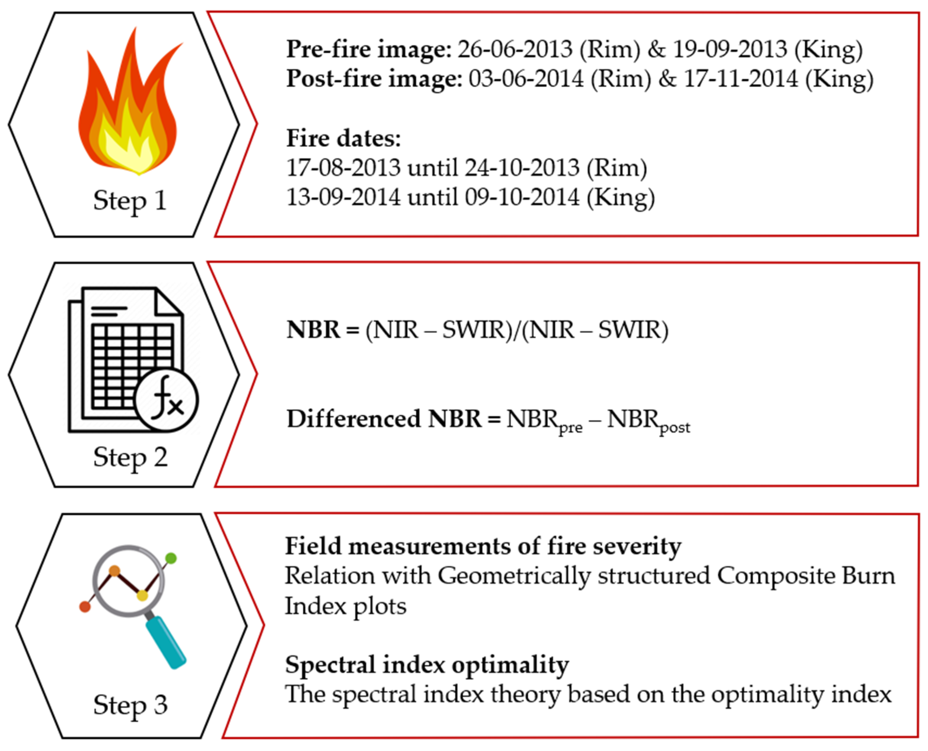
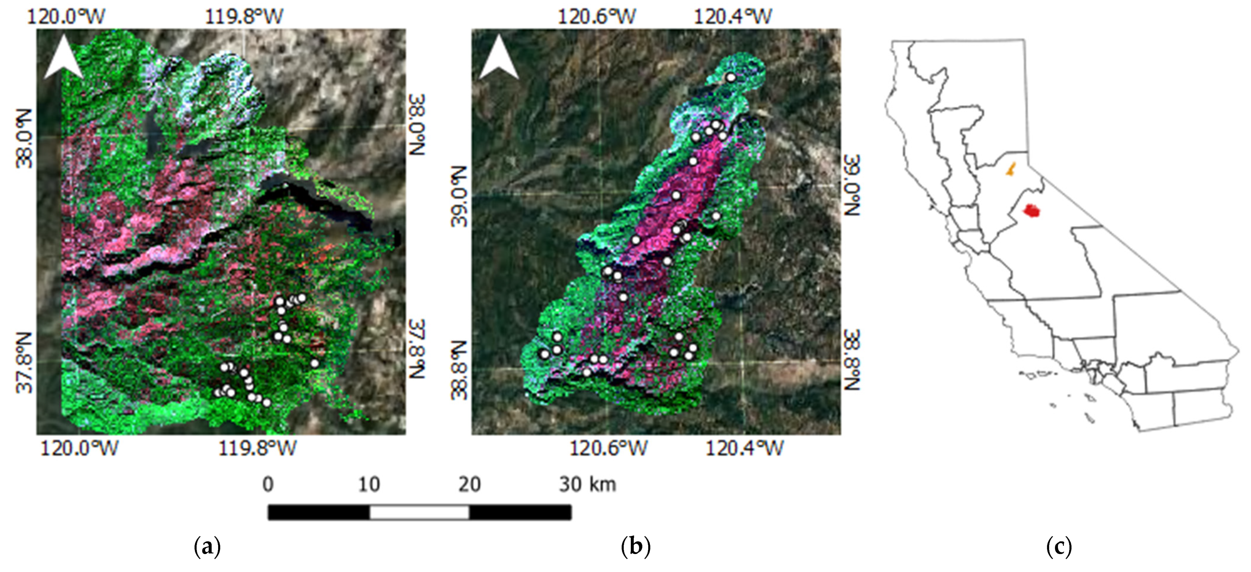
Our study included the 2013 Rim and 2014 King fires in California’s Sierra Nevada Mountain range (Appendix A, Figure A1). The Rim fire burned ~104,000 ha across Yosemite National Park and the Stanislaus National Forest (Appendix A, Figure A1a, Step 1 Figure 1). The King fire burned ~40,000 ha in the Eldorado National Forest (Appendix A, Figure A1b, Step 1 Figure 1). The fires burned through patchy vegetation dominated by dense mature forests of ponderosa pine (Pinus ponderosa), Douglas fir (Pseudotsuga menziesii), and incense cedar (Calocedrus decurrens) [28,42,43,44].

2.2. Airborne Visible/Infrared Imaging Spectrometer Imagery

The sensitivity of the hyperspectral dNBR to assess fire severity was evaluated using airborne imagery from the AVIRIS sensor. The AVIRIS sensor acquires narrowband data in 224 contiguous spectral channels that span the 0.4 μm to 2.5 μm spectral range [29]. The bandwidth of the AVIRIS sensor within the NIR spectral region is 9.4 nm, and within the SWIR spectral region, the bandwidth is 9.7 nm. Over the Rim fire, spectral imagery was acquired with a spatial resolution of 14.6 m. For the King fire, the spatial resolution was 14.8 m [29,32,45]. We calculated all unique hyperspectral dNBR combinations using the AVIRIS bands in the NIR and SWIR spectral regions. We excluded bands in the main water vapor absorption regions. This resulted in the exclusion of bands 33 to 36, 103 to 114, 142 to 143, and 153 to 168. In total, 156 bands were retained in this study, of which 60 were NIR bands and 96 were SWIR bands [28]. This allowed for 5760 unique dNBR combinations. We used Level 2 surface reflectance data [46]. The AVIRIS spectral channels were atmospherically corrected using the Atmosphere Removal Algorithm (ATREM) [47]. All surface reflectance bands were further topographically corrected using 1 m digital orthophoto images resampled to the AVIRIS resolution [46]. Prior to mosaicking, images were normalized to reduce discrepancies in bi-directional reflectance distribution functions using a modified version of the Canty normalization algorithm [45]. The images were acquired at near anniversary dates for both fires; thus, phenological differences between images were minimal (Step 1 Figure 1). The June 2013 AVIRIS acquisition over the Rim fire (pre-fire) covered roughly 64% of the fire perimeter with a two km buffer in the months preceding ignition. Post-fire coverage of the AVIRIS sensor approximates 96% of the fire perimeter, including the buffer. For the King fire, both pre- and post-fire flight lines fully covered the fire perimeter, including a two km buffer [46].

2.3. Field Measurements of Fire Severity

To assess in situ fire severity, we used the Geometrically structured Composite Burn Index (GeoCBI) protocol [40,41]. GeoCBI divides the ecosystem into five different strata using one substrate and four vegetation strata [10]. In each stratum, different fire severity characteristics, such as char height, percentage altered foliage, and soil and rock cover and color changes are rated. Fire severity is scored on a continuous scale between zero and three based on semi-quantitative expert judgement approach. Scores of zero represent unburned field plots, while a score of three marks a high fire severity plot. Based on the stratum averages and corresponding fractions of cover, plot-level fire severity is expressed by the strata weighted average. In total 85 plots were sampled across the Rim (n = 33) and King (n = 52) fires [42]. Two field data plots of the Rim fire campaign were excluded from our assessment, as they were outside the extent of the AVIRIS images. Field plot locations were chosen to represent the observed range of fire severity in mixed conifer forests. Furthermore, plots were selected in homogeneous areas with regards to pre-fire vegetation and fire severity; because of accessibility, plots were often sampled in vicinity of roads and trails but at least 100 m away from those.

2.4. Spectral Index Optimality

Spectral index optimality quantifies the index’s sensitivity to monitor a change of interest, in this case, fire-induced ecosystem changes [10,12]. The spectral optimality is thereby defined by the direction and magnitude of pixel displacements that form an unburned to a burned pixel, in reference to what an optimal pixel displacement in the bi-spectral space [38]. An optimal pixel displacement is perpendicular to the index isolines, while displacements along index isolines represent noise. Based on these pixel displacements, a spectral index optimality metric has been defined [14,42,44]. An optimality value of one denotes an optimally sensed bi-temporal pixel displacement, whereas an optimality value of zero means that the spectral index is insensitive to the bi-temporal pixel displacement.

2.5. Statistical Analysis

We retrieved the average surface reflectance over the field plots using three-by-three-pixel windows for which the coordinates of the centers of the field plots were located within the center pixels of the three-by-three windows. The center of each pixel window intersects with the recorded centroids of the GeoCBI 30 by 30 m field plot location. This approach reduces the effects of potential satellite misregistration [48].

Furthermore, to describe the relationship between the field measurements and remotely sensed dNBR we employed a non-linear saturated growth model [49]. Regression results were evaluated using the coefficient of determination R² and the root mean squared error (RMSE) as goodness-of-fit parameters. The optimality statistics of all burned pixels were evaluated for each index combination using the median statistic [42].

Ideally, the overall best-performing bi-spectral combination has a high correlation with field data and monitors the change of interest well. Both the regression R² and the median optimality strength tests in our assessment resulted in scores between zero and one. Hence, we used the mean scores across both strength tests to identify the overall ideal NIR–SWIR combination. Therefore, the overall performance of each index is a dimensionless score between zero and one. A performance score of one indicates a perfect relationship with field data and perfect monitoring of the change of interest. A score of zero means that there is no relationship with field data and complete insensitivity to fire-induced spectral changes.

3. Results

3.1. Relationships between Field and Airborne Data

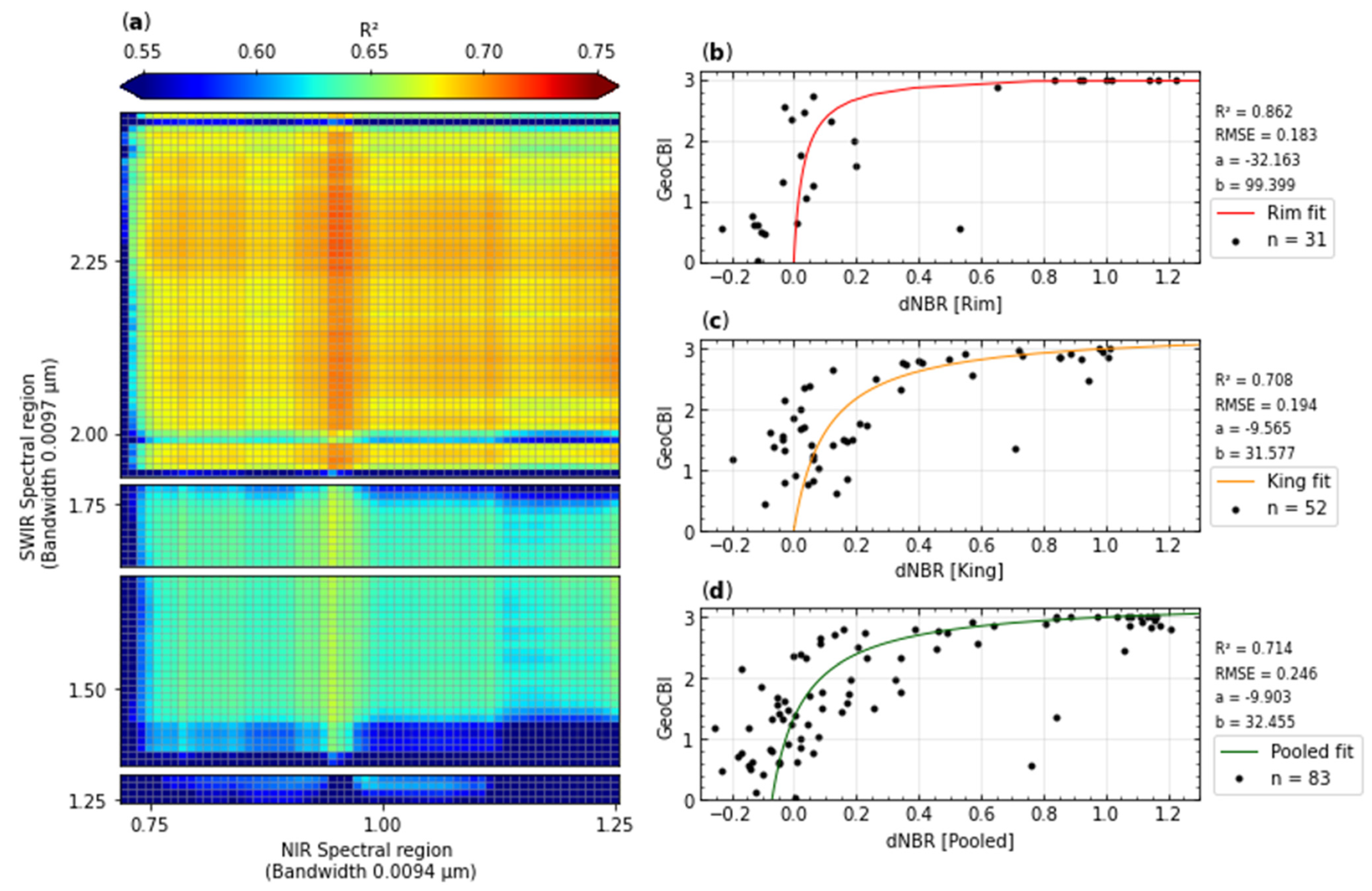
The best-performing dNBR index resulted in an R² of 0.71 (Figure 2). The optimal AVIRIS based index was constructed using band 63 (0.962 µm) and band 203 (2.246 µm) of the AVIRIS sensor (Figure 2a,d). Figure 2b,c show the strongest spectral index relationships with the GeoCBI for the individual fire scars. The Rim (n = 31) and King (n = 52) fires demonstrated reasonably strong (0.50 < R² < 0.80) to very strong (R² ≥ 0.80) relationships with the GeoCBI field data throughout the entire NIR–SWIR bi-spectral space (Appendix B, Figure A2). However, significant differences in the form of the relationships were observed between the two fire scars. There were differences in the location of the most optimal NIR and SWIR. The dNBR combination with the strongest relationship with field data for the Rim fire was constructed with bands 62 (NIR = 0.953 µm) and 224 (SWIR = 2.45 µm). This combination demonstrated a very strong relationship with GeoCBI, as it yielded an R² score of 0.86 (Figure 2b). The King fire’s best fitting dNBR returned a R² score of 0.71, using bands 96 (NIR = 1.25 µm) and 152 (SWIR = 1.774 µm).

3.2. dNBR Optimality

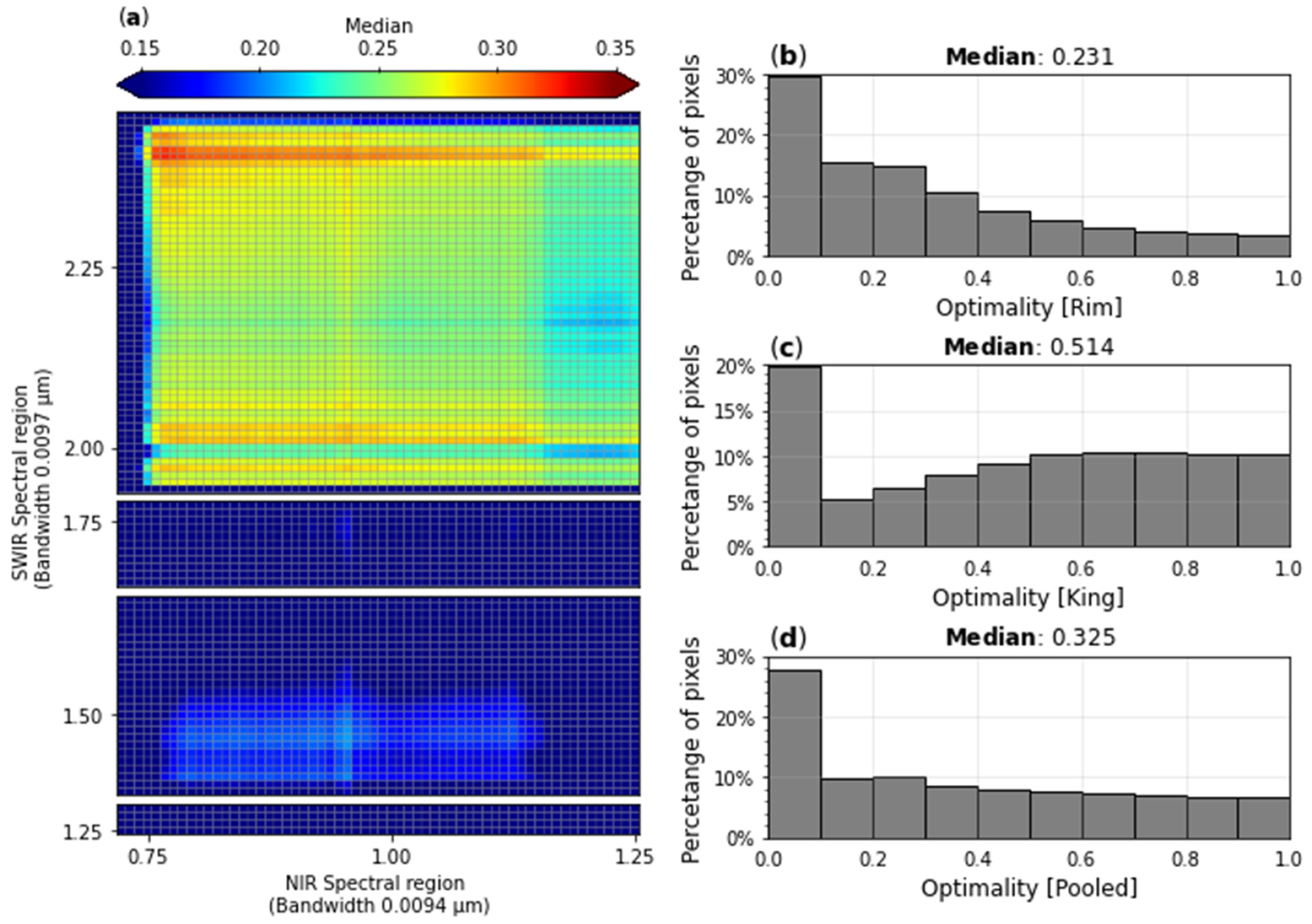
The median optimality of the best-performing dNBR was 0.23 over the Rim fire (NIR = 0.962 µm, SWIR = 2.004 µm) and 0.51 over the King fire (NIR = 0.765 µm, SWIR = 2.169 µm) (Figure 3b,c). Using data from both fires, the highest median optimality was 0.33 for the dNBR combination of the NIR band centered at 0.765 µm and the SWIR band centered at 2.382 µm (Figure 3a,d). Figure 3b–d show the histograms with the optimality values for the best-performing dNBR for the Rim fire, King fire, and both fires. Both datasets recorded many pixels with optimality values lower than 0.1. Moreover, the Rim and King fires display opposite trends with relationship to pixels optimality values higher than 0.1. The Rim fire showed a declining trend, where an inclining trend was recorded for the King fire toward more pixels with higher optimality values. Combining data from the Rim and King fires resulted in a slight declining trend for pixels with optimality values higher than 0.1.

3.3. Overall Performance

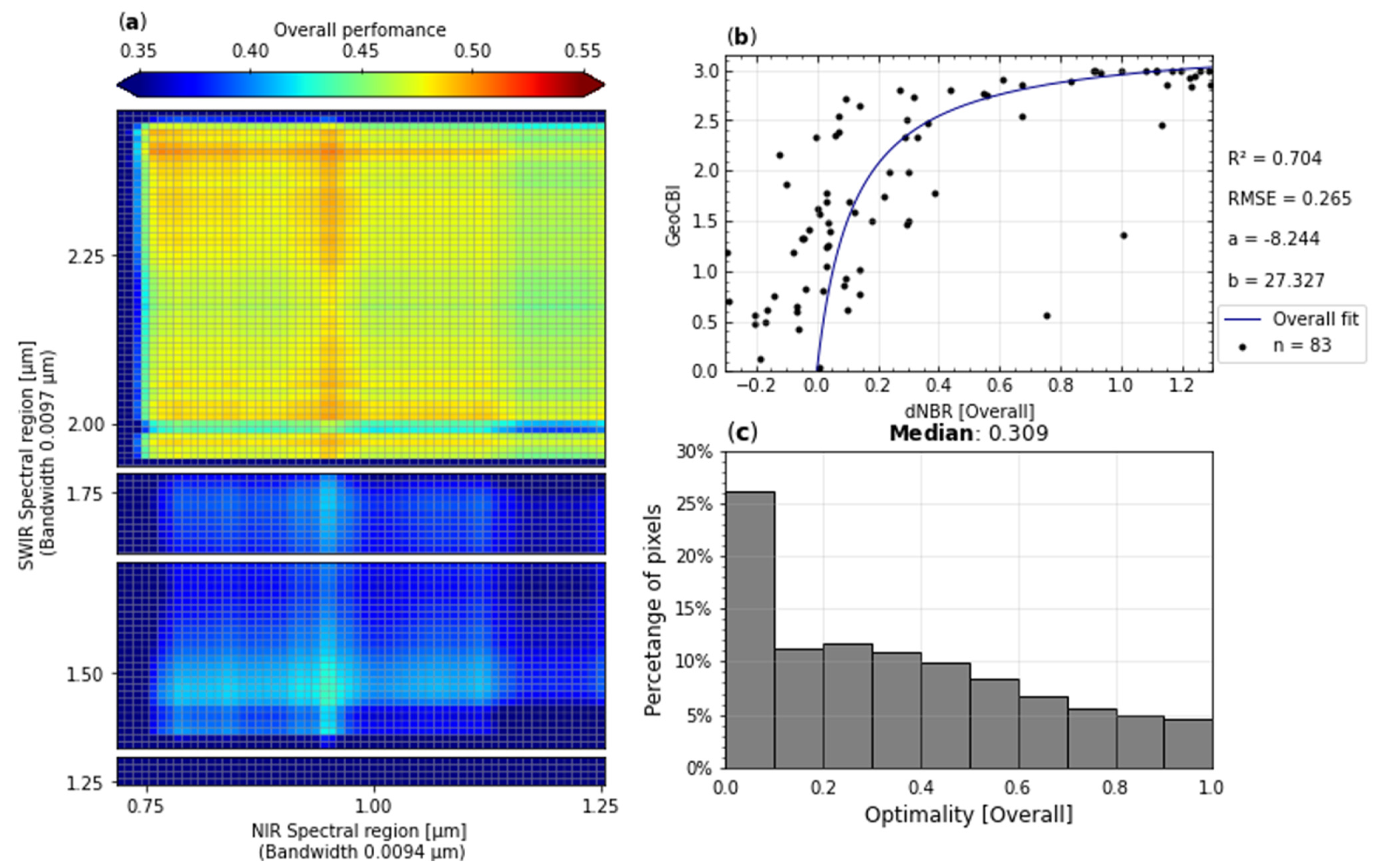
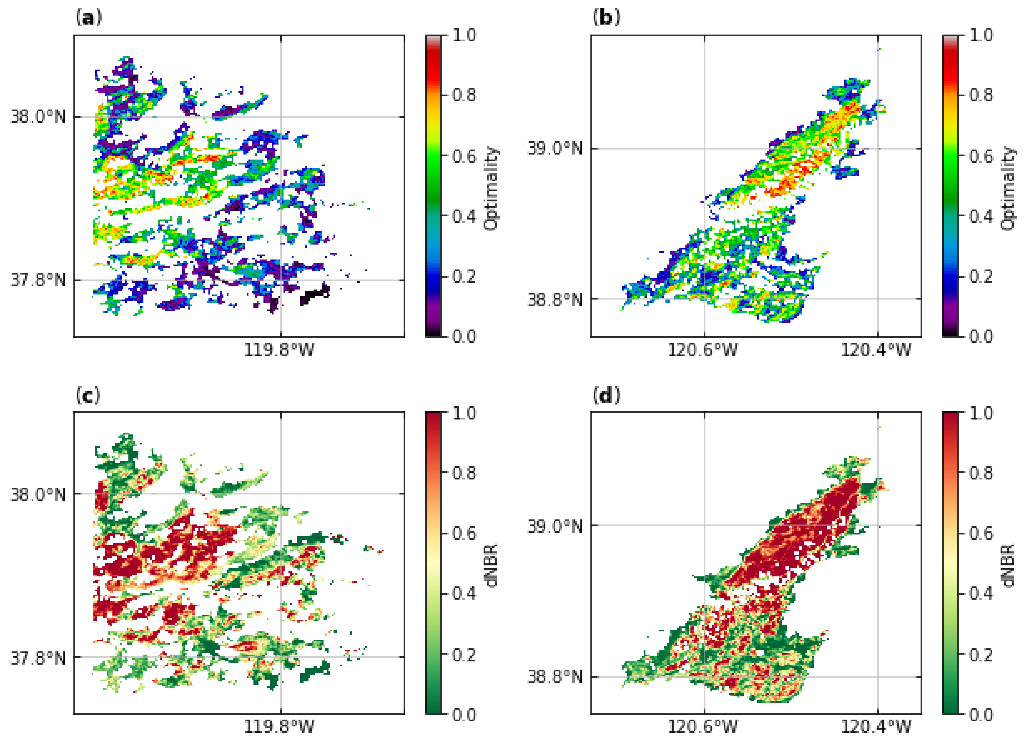
The hyperspectral dNBR that performed best in our analysis, considering both the relationship with field data and the spectral optimality of the index, was constructed with band 63 (NIR, centered at 0.962 µm) and band 218 (SWIR, centered at 2.382 µm) (Figure 4a). The dNBR yielded an R² score of 0.70 (Figure 4b). The median spectral optimality was 0.31 (Figure 4c). The field data exhibited dNBR values ranging from −0.318 to 1.335. Our model predictions encounter an RMSE of 0.27, which is roughly one-seventh of the total GeoCBI variation in our field data. The predicted GeoCBI values thus substantially diverged from the observations. The optimality maps of the best-performing hyperspectral dNBR are displayed in Figure 5a,b. The median optimality of the dNBR was 0.20 for the Rim fire (Figure 5a) and 0.46 for the King fire (Figure 5b).

The hyperspectral dNBR values were bi-temporally differenced (Step 2 Figure 1). These differenced maps are shown in Figure 5c,d. Furthermore, it is apparent that a significant number of pixels with a recorded optimality values lower than 0.2 correspond to unburned areas within the fire scar, as can be seen in the dNBR maps.

4. Discussion

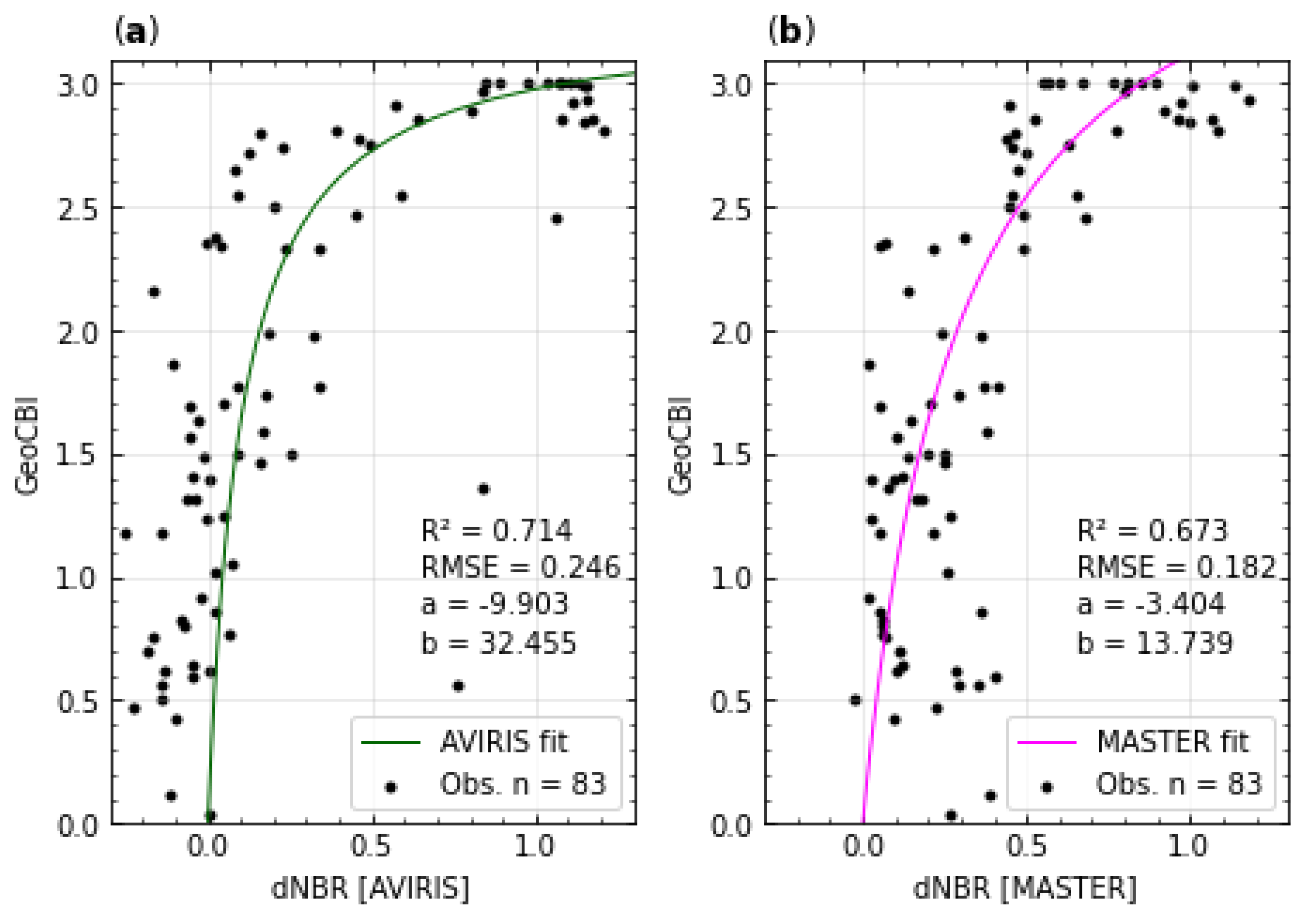
The results of the hyperspectral dNBR display strong relationships with GeoCBI field data for a temperate environment, such as California, USA. Depending on the studied datasets and fires, the best hyperspectral dNBR relationships with GeoCBI field resulted in R² of 0.70 (Figure 4). The model results fall within the ranges observed in previous GeoCBI–dNBR studies based on multispectral data [20,26,28]. The inter-comparison across different fires shows the same large variability in the form of relationships as confirmed in previous crossfire field data and airborne relationship studies [19,26,44,50]. Van Gerrevink and Veraverbeke (2021) [42] assessed the GeoCBI–dNBR relation over the same fires with multispectral data from MODIS/ASTER (Moderate Resolution Imaging Spectrometer/Advanced Spaceborne Thermal Emission and Reflection Radiometer) Airborne Simulator (MASTER) instrument. The hyperspectral dNBR (R² of 0.71) (Figure 2d) reported in this study slightly outperformed van Gerrevink and Veraverbeke’s multispectral dNBR (R² of 0.67) (Appendix C, Figure A3). The improved overall dNBR–GeoCBI form of relationship can be partly explained by the improvements across the Rim fire. Multispectral data yielded an R² of 0.52, whereas hyperspectral data results demonstrated an R² of 0.86 for the Rim fire. However, significant residual variability among the fitted models, as shown in Figure 4b,c, suggests relatively high uncertainty in estimated fire severity similar to earlier studies with multispectral data [26,28,46]. The uncertainty arises from several shortcomings inherent to the dNBR. For example, the dNBR is sensitive to non-fire induced spectral alterations [10,12]. Additionally, GeoCBI–dNBR models demonstrate asymptotic behavior. This demonstrates difficulties of the dNBR to differentiate between high severity plots [49].

In addition, our optimality results across the Rim and King fires re-affirm a large variability in dNBR optimality across fires [12,43]. The combined dataset recorded a median statistic of 0.33 for the best NIR–SWIR combination. The optimality results are highly comparable with the results presented by Roy et al. [12] and Escuin et al. [21]. Roy et al. [12] assessed the optimality of the dNBR from MODIS images over fires across different biomes; however, this analysis included unburned pixels. Their mean optimality result fell within the range of 0.24 to 0.33. Escuin et al. [21] conducted an optimality assessment of fire severity using the dNBR from Landsat imagery. Including unburned pixels resulted in a decrease in median optimality scores between 0.09 and 0.49 [21]. Both Roy et al. [12] and Escuin et al. [21] reported a significant percentage of pixels with an optimality score lower than 0.1, when unburned pixels were incorporated into their optimality assessments. Our hyperspectral dNBR optimality analysis reported similar percentages of pixels with an optimality score lower than 0.1. The dNBR maps in Figure 5c,d show many pixels with low dNBR values that approach zero. These low dNBR pixels were enclosed in the fire perimeter, and this suggests that unburned pixels with consequent low optimality were included in our analysis. The low performance of wavebands located between 1.25 µm and 1.78 µm is consistent with the pre- and post-fire differenced AVIRIS spectral reflectance across all fire severity categories from van Wagtendonk et al. (2004) [23].

Van Gerrevink and Veraverbeke [42] conducted an optimality assessment using the dNBR from multispectral MASTER imagery over the same fires. They also found a comparably high percentage of pixels with optimality scores lower than 0.1; however, the median optimality values exceeded the values of our current hyperspectral study. The median spectral optimality was 0.56 for the Rim fire and 0.60 for the King fire [42]. The difference in optimality distributions may be caused by a proportional difference in cloud cover between the MASTER and AVIRIS imagery. Cloud cover can significantly affect the optimality performance. Large cloudy areas constrained our optimality analysis, because of which several patches of pixels were excluded from the optimality analysis. Inaccuracies in the cloud cover map that we used may have resulted in the inclusion of cloud-affected pixels in our analysis. This seems especially apparent for the Rim fire, where many cloud-affected areas were present (Figure 5a,b). The number of cloud-affected pixels partly explains the significant discrepancy in the median statistic between the two fires. Moreover, hyperspectral imagery is inherently more sensitive to noise due to its narrow bandwidth [50,51]. This lower signal-to-noise ratio with hyperspectral imagery may have further deteriorated optimality performances.

Van Wagtendonk et al. [23] provided a rare example that capitalized upon earlier pre- and post-fire hyperspectral airborne image acquisitions for fire severity assessments. They compared AVIRIS and Landsat detection capabilities over the 2001 Hoover fire in California, USA. The hyperspectral results agreed well with fire severity detections using multispectral sensors but unveiled no increased sensitivity of the hyperspectral assessment compared to the multispectral assessment [23,27]. To derive the hyperspectral dNBR, van Wagtendonk et al. [23] investigated one hyperspectral band combination. This selection was based on the maximum bi-temporal response in spectral reflectance regions. The AVIRIS bands 47 (NIR, centered at 0.788 µm) and 210 (SWIR, centered at 2.370 µm) were selected for their hyperspectral dNBR [23]. Additionally, they conclude that the NIR and SWIR Landsat ETM+ bands were not optimally located for fire severity assessments as other spectral regions sampled by AVIRIS demonstrated great potential for fire severity quantifications. Our study extends the work of van Wagtendonk et al. [23], as it assesses the full potential of all possible hyperspectral NIR–SWIR bi-spectral combinations. Landsat 8 and Sentinel-2 are currently the most commonly used broadband sensors for fire severity assessments [16,18]. For Landsat 8, the dNBR is calculated using band 5 (NIR, between 0.85 and 0.88 µm) and band 7 (NIR, between 2.11 and 2.29 µm). For Sentinel-2, the equivalent bands are band 8A (NIR, between 0.855 µm and 0.875 µm) and band 12 (SWIR, between 2.100 µm and 2.280 µm). Our hyperspectral analysis revealed other responsive portions within the NIR–SWIR bi-spectral space, which are not sampled by current broadband sensors like Landsat 8 and Sentinel-2. The hyperspectral dNBR with the best performance was constructed with longer NIR (centered at 0.962 µm) and SWIR (centered at 2.382 µm) wavelengths than those available from Landsat 8 and Sentinel-2 (Figure 4a). The spectral location of the SWIR band from our best-performing index is remarkably close to the SWIR band location identified by van Wagtendonk et al. [23] using the maximum bi-temporal response signatures. The spectral locations of the best-performing NIR band is more different between our study and that of van Wagtendonk et al. [23]. However, the bi-temporal response signature of AVIRIS sensor demonstrates the potential for sampling NIR spectral bands in vicinity of 0.912 µm [13,23]. Van Wagtendonk et al. [23] did not evaluate the use of NIR bands at these longer wavelengths in the context of change detection. Therefore, our study re-affirms the findings of van Wagtendonk et al. [23] that hyperspectral sensors that image outside the broadband ranges may outperform fire severity assessments from multispectral broadband sensors.

Despite the relative success of the dNBR approach in fire severity mapping, our analyses of the hyperspectral dNBR showed large variability in the form of relationships with field data between fires (Figure 2) [19,20,26,50]. The spectral sensitivity of the SWIR region to difference in soil brightness and moisture conditions partly explains the spatial and temporal variability in the dNBR response [12,52]. While the dNBR is a powerful proxy that captures the bio-physical properties of fire-induced change to the landscape, it only uses spectral information from two bands [10,19,24]. By doing so, dNBR fire severity studies do not capitalize on the advantage of the wealth of available spectral information. Spectral mixture analysis (SMA) has been applied in multispectral post-fire fire severity studies; however, some studies have capitalized upon hyperspectral data [27,28,53,54,55,56,57,58,59,60]. The main advantage of SMA in fire severity assessments is that it does not require field data calibrations as it quantifies the abundance of ground cover classes. The estimates of green vegetation and charcoal fractions correlate significantly with ground measurements of fire severity, providing a valuable alternative in the absence of pre- and post-fire hyperspectral pairs [17,24,29]. Tane et al. [28] mapped the fire severity over the Rim fire from hyperspectral image using Multiple Endmember Spectral Mixture Analysis (MESMA), which is a SMA technique that accounts for end-member variability. The fractional cover maps derived from MESMA were validated with high-resolution WorldView-2 imagery. A comparison with the high-resolution fire severity estimates from Worldview-2 resulted in reasonably strong relationships with the MESMA-derived ash cover (R² of 0.741). This performance is similar to our relationship between the hyperspectral dNBR and the GeoCBI. Furthermore, light detection and ranging (LiDAR) imagery can be used to derive the waveform area relative change (WARC) metric [61]. This newly developed fire severity assessment technique capitalizes upon changes in vegetation structure among changes in leaf and soil colors. The WARC metric has successfully been validated over the King fire. Synergistic use of spectral indices and LiDAR could improve the assessment of post-fire damages and contribute to a more detailed long-term fire severity evaluation [61].

Potential inaccuracies that hampered our analysis may emerge from both field and remotely sensed observations [42]. GeoCBI field data analysis preferentially requires a stratified sampling approach. Therefore, the number of plots per fuel type should be closely correlated with the proportion of the total burned area for each fuel type. Due to accessibility limitations, we were unable to fulfill this criterion. Secondly, the divergence of remotely sensed estimates and in situ field measurements of fire severity is partially because both observation methods are imperfect proxies of fire severity. Field data observations of GeoCBI are based on semi-quantitative judgements approaches, thus inherently prone to some degree of subjectivity, specifically with assessments by different field teams, as was the case in our study. Our optimality results revealed a substantial amount of noise within the spectral indices, as the median statistics of both fires were substantially lower than the optimal score of one. The occurrence of noise in remotely sensed change detection can result from minor differences in phenology between image acquisitions, and imperfections raised in the pre-processing of images, including identifying and removing clouds from the analysis. Hyperspectral imagery in multi-temporal differenced fire severity assessments has long been limited by complexities of airborne data acquisition. As such, pre- and post-fire hyperspectral imagery over ground-truthed fires have remained rare [24,27,33]. Our study is therefore timely, as it identifies opportunities that may arise from hyperspectral fire severity mapping now that more frequent pre- and post-fire imagery will become available from ongoing (PRISMA, HISUI) and upcoming (EnMAP, SBG, SHALOM) spaceborne hyperspectral missions.

5. Conclusions

Based on relationships with field measurements and optimality of spectral index optimality, our study is one of the first to assess the hyperspectral sensitivity of the dNBR for assessing fire severity. Broadly, our results re-affirm the strength of the dNBR for capturing large parts of the variability observed in field observation of fire severity, as demonstrated earlier with multispectral assessments. However, we also found that the spectral locations of the NIR and SWIR bands of the best-performing hyperspectral dNBR combination are positioned outside the wavelength range of the bands that constitute the dNBR from spaceborne multispectral missions such as Landsat 8 and Sentinel-2. We therefore tested 5760 dNBR combinations in total, using 60 unique NIR and 96 SWIR spectral bands. The overall best-performing hyperspectral dNBR was based on band 63 (NIR, centered at 0.962 µm) and band 218 (SWIR, centered at 2.382 µm). Our study made use of pre- and post-fire airborne acquisitions over the Rim and King fires in California from the AVIRIS sensor. By doing so, this study is the first to evaluate full potential of the NIR–SWIR bi-spectral space with hyperspectral data for assessing fire severity. With the increasing availability of hyperspectral data from recently launched and upcoming spaceborne imaging spectroradiometers, the calculation of the hyperspectral dNBR will become more widespread. We provided a first assessment of the hyperspectral dNBR over two fires in temperate forest ecosystems, and further analysis should evaluate whether hyperspectral sensitivity may be different across ecosystems.

References

- Harris, S.; Veraverbeke, S.; Hook, S. Evaluating spectral indices for assessing fire severity in chaparral ecosystems (Southern California) using modis/aster (MASTER) airborne simulator data. Remote Sens. 2011, 3, 2403–2419. [Google Scholar] [CrossRef] [Green Version]
- Hammill, K.A.; Bradstock, R.A. Remote sensing of fire severity in the Blue Mountains: Influence of vegetation type and inferring fire intensity. Int. J. Wildland Fire 2006, 15, 213–226. [Google Scholar] [CrossRef]
- Chafer, C.J. A comparison of fire severity measures: An Australian example and implications for predicting major areas of soil erosion. Catena 2008, 74, 235–245. [Google Scholar] [CrossRef]
- Chafer, C.J.; Noonan, M.; Macnaught, E. The post-fire measurement of fire severity and intensity in the Christmas 2001 Sydney wildfires. Int. J. Wildland Fire 2004, 13, 227–240. [Google Scholar] [CrossRef]
- González-Alonso, F.; Merino-De-Miguel, S.; Roldán-Zamarrón, A.; García-Gigorro, S.; Cuevas, J.M. MERIS full resolution data for mapping level-of-damage caused by forest fires: The Valencia de Alcántara event in August 2003. Int. J. Remote Sens. 2007, 28, 797–809. [Google Scholar] [CrossRef]
- Keeley, J.E. Fire intensity, fire severity and burn severity: A brief review and suggested usage. Int. J. Wildland Fire 2009, 18, 116–126. [Google Scholar] [CrossRef]
- Brewer, C.K.; Winne, J.C.; Redmond, R.L.; Opitz, D.W.; Mangrich, M.V. Classifying and mapping wildfire severity. Photogramm. Eng. Remote Sens. 2005, 71, 1311–1320. [Google Scholar] [CrossRef] [Green Version]
- Jain, T.B. Tongue-Tied: Confused meanings for common fire terminology can lead to fuels mismanagement. Wildfire 2004, July/August, 22–26. [Google Scholar]
- Lentile, L.B.; Holden, Z.A.; Smith, A.M.S.; Falkowski, M.J.; Hudak, A.T.; Morgan, P.; Lewis, S.A.; Gessler, P.E.; Benson, N.C. Remote sensing techniques to assess active fire characteristics and post-fire effects. Int. J. Wildland Fire 2006, 15, 319–345. [Google Scholar] [CrossRef]
- Veraverbeke, S.S.N.; Verstraeten, W.W.; Lhermitte, S.; Goossens, R. Evaluating Landsat Thematic Mapper spectral indices for estimating burn severity of the 2007 Peloponnese wildfires in Greece. Int. J. Wildland Fire 2010, 19, 558–569. [Google Scholar] [CrossRef] [Green Version]
- Morgan, P.; Keane, R.E.; Dillon, G.K.; Jain, T.B.; Hudak, A.T.; Karau, E.C.; Sikkink, P.G.; Holden, Z.A.; Strand, E.K. Challenges of assessing fire and burn severity using field measures, remote sensing and modelling. Int. J. Wildland Fire 2014, 23, 1045–1060. [Google Scholar] [CrossRef] [Green Version]
- Roy, D.P.; Boschetti, L.; Trigg, S.N. Remote sensing of fire severity: Assessing the performance of the normalized burn ratio. IEEE Geosci. Remote Sens. Lett. 2006, 3, 112–116. [Google Scholar] [CrossRef] [Green Version]
- Veraverbeke, S.S.N.; Stavros, E.N.; Hook, S.J. Assessing fire severity using imaging spectroscopy data from the Airborne Visible/Infrared Imaging Spectrometer (AVIRIS) and comparison with multispectral capabilities. Remote Sens. Environ. 2014, 154, 153–163. [Google Scholar] [CrossRef]
- Eidenshink, J.; Schwind, B.; Brewer, K.; Zhu, Z.-L.; Quayle, B.; Howard, S. A project for monitoring trends in burn severity. Fire Ecol. 2007, 3, 3–21. [Google Scholar] [CrossRef]
- Epting, J.; Verbyla, D.; Sorbel, B. Evaluation of remotely sensed indices for assessing burn severity in interior Alaska using Landsat TM and ETM+. Remote Sens. Environ. 2005, 96, 328–339. [Google Scholar] [CrossRef]
- French, N.H.F.; Kasischke, E.S.; Hall, R.J.; Murphy, K.A.; Verbyla, D.L.; Hoy, E.E.; Allen, J.L. Using Landsat data to assess fire and burn severity in the North American boreal forest region: An overview and summary of results. Int. J. Wildland Fire 2008, 17, 443–462. [Google Scholar] [CrossRef]
- García, M.J.L.; Caselles, V. Mapping burns and natural reforestation using thematic mapper data. Geocarto Int. 1991, 6, 31–37. [Google Scholar] [CrossRef]
- Delcourt, C.J.F.; Combee, A.; Izbicki, B.; Mack, M.C.; Maximov, T.; Petrov, R.; Rogers, B.M.; Scholten, R.C.; Shestakova, T.A.; Van Wees, D.; et al. Evaluating the Differenced Normalized Burn Ratio for Assessing Fire Severity Using Sentinel-2 Imagery in Northeast Siberian Larch Forests. Remote Sens. 2021, 13, 2311. [Google Scholar] [CrossRef]
- Saulino, L.; Rita, A.; Migliozzi, A.; Maffei, C.; Allevato, E.; Garonna, A.P.; Saracino, A. Detecting Burn Severity across Mediterranean Forest Types by Coupling Medium-Spatial Resolution Satellite Imagery and Field Data. Remote Sens. 2020, 12, 741. [Google Scholar] [CrossRef] [Green Version]
- De Santis, A.; Chuvieco, E. Burn severity estimation from remotely sensed data: Performance of simulation versus empirical models. Remote Sens. Environ. 2007, 108, 422–435. [Google Scholar] [CrossRef]
- Escuin, S.; Navarro, R.; Fernández, P. Fire severity assessment by using NBR (Normalized Burn Ratio) and NDVI (Normalized Difference Vegetation Index) derived from LANDSAT TM/ETM images. Int. J. Remote Sens. 2008, 29, 1053–1073. [Google Scholar] [CrossRef]
- Murphy, K.A.; Reynolds, J.H.; Koltun, J.M. Evaluating the ability of the differenced Normalized Burn Ratio (dNBR) to predict ecologically significant burn severity in Alaskan boreal forests. Int. J. Wildland Fire 2008, 17, 490–499. [Google Scholar] [CrossRef]
- Van Wagtendonk, J.W.; Root, R.R.; Key, C.H. Comparison of AVIRIS and Landsat ETM+ detection capabilities for burn severity. Remote Sens. Environ. 2004, 92, 397–408. [Google Scholar] [CrossRef]
- Lu, P.; Wang, L.; Niu, Z.; Li, L.; Zhang, W. Prediction of soil properties using laboratory VIS—NIR spectroscopy and Hyperion imagery. J. Geochem. Explor. 2013, 132, 26–33. [Google Scholar] [CrossRef]
- Wang, J.; He, T.; Lv, C.; Chen, Y.; Jian, W. International Journal of Applied Earth Observation and Geoinformation Mapping soil organic matter based on land degradation spectral response units using Hyperion images. Int. J. Appl. Earth Obs. Geoinf. 2010, 12, S171–S180. [Google Scholar] [CrossRef]
- Schaepman, M.E.; Ustin, S.L.; Plaza, A.J.; Painter, T.H.; Verrelst, J.; Liang, S. Earth system science related imaging spectroscopy-An assessment. Remote Sens. Environ. 2009, 113, S123–S137. [Google Scholar] [CrossRef]
- Veraverbeke, S.S.N.; Dennison, P.; Gitas, I.; Hulley, G.; Kalashnikova, O.; Katagis, T.; Kuai, L.; Meng, R.; Roberts, D.; Stavros, N. Hyperspectral remote sensing of fire: State-of-the-art and future perspectives. Remote Sens. Environ. 2018, 216, 105–121. [Google Scholar] [CrossRef]
- Tane, Z.; Roberts, D.; Veraverbeke, S.; Casas, Á.; Ramirez, C.; Ustin, S. Evaluating endmember and band selection techniques for multiple endmember spectral mixture analysis using post-fire imaging spectroscopy. Remote Sens. 2018, 10, 389. [Google Scholar] [CrossRef] [Green Version]
- Green, R.O.; Eastwood, M.L.; Sarture, C.M.; Chrien, T.G.; Aronsson, M.; Chippendale, B.J.; Faust, J.A.; Pavri, B.E.; Chovit, C.J.; Solis, M. Imaging spectroscopy and the airborne visible/infrared imaging spectrometer (AVIRIS). Remote Sens. Environ. 1998, 65, 227–248. [Google Scholar] [CrossRef]
- Stavros, E.N.; Tane, Z.; Kane, V.R.; Veraverbeke, S.; McGaughey, R.J.; Lutz, J.A.; Ramirez, C.; Schimel, D. Unprecedented remote sensing data over King and Rim megafires in the Sierra Nevada Mountains of California. Ecology 2016, 97, 3244. [Google Scholar] [CrossRef]
- Pearlman, J.S.; Member, S.; Barry, P.S.; Segal, C.C.; Shepanski, J.; Beiso, D.; Carman, S.L. Hyperion, a Space-Based Imaging Spectrometer. IEEE Trans. Geosci. Remote Sens. 2003, 41, 1160–1173. [Google Scholar] [CrossRef]
- Middleton, E.M.; Ungar, S.G.; Mandl, D.J.; Ong, L.; Frye, S.W.; Campbell, P.E.; Landis, D.R.; Young, J.P.; Pollack, N.H. The earth observing one (EO-1) satellite mission: Over a decade in space. IEEE J. Sel. Top. Appl. Earth Obs. Remote Sens. 2013, 6, 243–256. [Google Scholar] [CrossRef]
- Labate, D.; Ceccherini, M.; Cisbani, A.; De Cosmo, V.; Galeazzi, C.; Giunti, L.; Melozzi, M.; Pieraccini, S.; Stagi, M. The PRISMA payload optomechanical design, a high performance instrument for a new hyperspectral mission. Acta Astronaut. 2009, 65, 1429–1436. [Google Scholar] [CrossRef]
- Iwasaki, A.; Ohgi, N.; Tanii, J.; Kawashima, T.; Inada, H. Hyperspectral Imager Suite (HISUI) -Japanese hyper-multi spectral radiometer. In Proceedings of the 2011 IEEE International Geoscience and Remote Sensing Symposium, Vancouver, BC, Canada, 24–29 July 2011; pp. 1025–1028. [Google Scholar] [CrossRef]
- Stuffler, T.; Kaufmann, C.; Hofer, S.; Förster, K.P.; Schreier, G.; Mueller, A.; Eckardt, A.; Bach, H.; Penné, B.; Benz, U.; et al. The EnMAP hyperspectral imager-An advanced optical payload for future applications in Earth observation programmes. Acta Astronaut. 2007, 61, 115–120. [Google Scholar] [CrossRef]
- Cawse-Nicholson, K.; Townsend, P.A.; Schimel, D.; Assiri, A.M.; Blake, P.L.; Buongiorno, M.F.; Campbell, P.; Carmon, N.; Casey, K.A.; Correa-Pabón, R.E.; et al. NASA’s surface biology and geology designated observable: A perspective on surface imaging algorithms. Remote Sens. Environ. 2021, 257, 112349. [Google Scholar] [CrossRef]
- Feingersh, T.; Ben Dor, E. SHALOM—A Commercial Hyperspectral Space Mission. Opt. Payloads Space Mission. 2015, 247–263. [Google Scholar] [CrossRef]
- Verstraete, M.M.; Pinty, B. Designing optimal spectral indexes for remote sensing applications. IEEE Trans. Geosci. Remote Sens. 1996, 34, 1254–1265. [Google Scholar] [CrossRef]
- Thenkabail, P.S.; Smith, R.B.; De Pauw, E. Evaluation of narrowband and broadband vegetation indices for determining optimal hyperspectral wavebands for agricultural crop characterization. Photogramm. Eng. Remote Sens. 2002, 68, 607–621. [Google Scholar]
- De Santis, A.; Chuvieco, E. GeoCBI: A modified version of the Composite Burn Index for the initial assessment of the short-term burn severity from remotely sensed data. Remote Sens. Environ. 2009, 113, 554–562. [Google Scholar] [CrossRef]
- Key, C.H.; Benson, N.C. Landscape Assessment (LA) sampling and analysis methods. In USDA Forest Service—General Technical Report RMRS-GTR; USDA Forest Service, Rocky Mountain Research Station: Fort Collins, CO, USA, 2006. [Google Scholar]
- van Gerrevink, M.J.; Veraverbeke, S. Evaluating the near and mid infrared bi-spectral space for assessing fire severity and comparison with the differenced normalized burn ratio. Remote Sens. 2021, 13, 695. [Google Scholar] [CrossRef]
- Stavros, E.N.; Coen, J.; Peterson, B.; Singh, H.; Kennedy, K.; Ramirez, C.; Schimel, D. Use of imaging spectroscopy and LIDAR to characterize fuels for fire behavior prediction. Remote Sens. Appl. Soc. Environ. 2018, 11, 41–50. [Google Scholar] [CrossRef]
- Casas, Á.; García, M.; Siegel, R.B.; Koltunov, A.; Ramírez, C.; Ustin, S. Burned forest characterization at single-tree level with airborne laser scanning for assessing wildlife habitat. Remote Sens. Environ. 2016, 175, 231–241. [Google Scholar] [CrossRef] [Green Version]
- Canty, M.J.; Nielsen, A.A. Automatic radiometric normalization of multitemporal satellite imagery with the iteratively re-weighted MAD transformation. Remote Sens. Environ. 2008, 112, 1025–1036. [Google Scholar] [CrossRef] [Green Version]
- Stavros, E.N.; Tane, Z.; Kane, V.R.; Veraverbeke, S.S.N.; McGaughey, R.; Lutz, J.A.; Ramirez, C.; Schimel, D.S. Remote Sensing Data Before and After California Rim and King Forest Fires, 2010–2015; ORNL DAAC: Oak Ridge, TN, USA, 2016. [Google Scholar] [CrossRef]
- Gao, B.; Goetz, A.F.H. Column atmospheric water vapor and vegetation liquid water retrievals from airborne imaging spectrometer data. J. Geophys. Res. 1990, 95, 3549–3564. [Google Scholar] [CrossRef]
- Ahern, F.J.; Erdle, T.; Maclean, D.A.; Kneppeck, I.D. A quantitative relationship between forest growth rates and Thematic Mapper reflectance measurements. Int. J. Remote Sens. 1991, 12, 387–400. [Google Scholar] [CrossRef]
- Hall, R.J.; Freeburn, J.T.; De Groot, W.J.; Pritchard, J.M.; Lynham, T.J.; Landry, R. Remote sensing of burn severity: Experience from western Canada boreal fires. Int. J. Wildland Fire 2008, 17, 476–489. [Google Scholar] [CrossRef]
- Plaza, A.; Plaza, J.; Paz, A.; Sánchez, S. Parallel Hyperspectral Image and Signal Processing [Applications Corner]. IEEE Signal Process. Mag. 2011, 28, 119–126. [Google Scholar] [CrossRef]
- Landgrebe, D.A. Hyperspectral data analysis procedures with reduced sensitivity to noise. In Proceedings of the Atmospheric Correction of Landsat Imagery, Torrance, CA, USA, 29 June–1 July 1993. NASA Contractor Report. [Google Scholar]
- Smith, A.M.S.; Eitel, J.U.H.; Hudak, A.T. Spectral analysis of charcoal on soils implications. Int. J. Wildland Fire 2010, 19, 976–983. [Google Scholar] [CrossRef]
- Veraverbeke, S.; Hook, S.J. Evaluating spectral indices and spectral mixture analysis for assessing fire severity, combustion completeness and carbon emissions. Int. J. Wildland Fire 2013, 22, 707–720. [Google Scholar] [CrossRef]
- Quintano, C.; Fernández-Manso, A.; Roberts, D.A. Multiple Endmember Spectral Mixture Analysis (MESMA) to map burn severity levels from Landsat images in Mediterranean countries. Remote Sens. Environ. 2013, 136, 76–88. [Google Scholar] [CrossRef]
- Lewis, S.A.; Hudak, A.T.; Ottmar, R.D.; Robichaud, P.R.; Lentile, L.B.; Hood, S.M.; Cronan, J.B.; Morgan, P. Using hyperspectral imagery to estimate forest floor consumption from wildfire in boreal forests of Alaska, USA. Int. J. Wildland Fire 2011, 20, 255–271. [Google Scholar] [CrossRef] [Green Version]
- Kokaly, R.F.; Rockwell, B.W.; Haire, S.L.; King, T.V.V. Characterization of post-fire surface cover, soils, and burn severity at the Cerro Grande Fire, New Mexico, using hyperspectral and multispectral remote sensing. Remote Sens. Environ. 2007, 106, 305–325. [Google Scholar] [CrossRef]
- Lewis, S.A.; Lentile, L.B.; Hudak, A.T.; Robichaud, P.R.; Morgan, P.; Bobbitt, M.J. Mapping Ground Cover Using Hyperspectral Remote Sensing after the 2003 Simi and Old Wildfires in Southern California. Fire Ecol. 2007, 3, 109–128. [Google Scholar] [CrossRef]
- Lewis, S.A.; Wu, J.Q.; Robichaud, P.R. Assessing burn severity and comparing soil water repellency, Hayman Fire, Colorado. Hydrol. Process. 2006, 20, 1–16. [Google Scholar] [CrossRef]
- Lewis, S.A.; Hudak, A.T.; Robichaud, P.R.; Morgan, P.; Satterberg, K.L.; Strand, E.K.; Smith, A.M.S.; Zamudio, J.A.; Lentile, L.B. Indicators of burn severity at extended temporal scales: A decade of ecosystem response in mixed-conifer forests of western Montana. Int. J. Wildland Fire 2017, 26, 755–771. [Google Scholar] [CrossRef] [Green Version]
- Robichaud, P.R.; Lewis, S.A.; Laes, D.Y.M.; Hudak, A.T.; Kokaly, R.F.; Zamudio, J.A. Postfire soil burn severity mapping with hyperspectral image unmixing. Remote Sens. Environ. 2007, 108, 467–480. [Google Scholar] [CrossRef] [Green Version]
- García, M.J.L.; North, P.; Viana-Soto, A.; Stavros, N.E.; Rosette, J.; Martín, M.P.; Franquesa, M.; González-Cascón, R.; Riaño, D.; Becerra, J.; et al. Evaluating the potential of LiDAR data for fire damage assessment: A radiative transfer model approach. Remote Sens. Environ. 2020, 247. [Google Scholar] [CrossRef]
Figure 1.
Methodological workflow. The components highlight three different phases of this study: Step 1 includes the data retrieval and pre-processing, Step 2 represents the spectral band selections and index construction, and Step 3 describes the index evaluation approaches using field measurements of fire severity and the spectral index optimality theory.
Figure 2.
Regression results of the saturated growth model for GeoCBI field data in relation to spectral indices. (a) Matrix of the coefficient of determination results R2 of all hyperspectral dNBR combinations. (b) Scatter plot and regression line between the GeoCBI field data and the best-performing dNBR index for the Rim fire (NIR = 0.953 µm, SWIR = 2.45 µm). (c) Scatter plot and regression line between the GeoCBI field data and the best-performing dNBR index for the King fire (NIR = 1.25 µm, SWIR = 1.774 µm). (d) Scatter plot and regression line between the GeoCBI field data and the best-performing dNBR index across the pooled data set (NIR = 0.962 µm, SWIR = 2.246 µm). The white spaces in panel (a) represents the wavelength at which bands were excluded. (NIR: near infrared, SWIR: short-wave infrared, dNBR: differenced normalized burn ratio, GeoCBI: geometrically structured composite burn index).
Figure 3.
Optimality results of the hyperspectral differenced normalized burn ratio (dNBR). Color scale refers to the median optimality. (a) Matrix of the median optimality of all dNBR combinations. (b) Histogram of the highest dNBR optimality over the Rim fire (NIR = 0.962 µm, SWIR = 2.004 µm). (c) Histogram of the highest dNBR optimality over the King fire (NIR = 0.765 µm, SWIR = 2.169 µm). (d) Histogram of the highest dNBR (optimality over both fire scars) (NIR = 0.765 µm, SWIR = 2.382 µm). The white spaces in panel (a) represent the wavelength at which bands were excluded. (NIR: near infrared, SWIR: short-wave infrared).
Figure 4.
Overall performance of the hyperspectral differenced Normalized Burn Ratio (dNBR) over the pooled data set. The color scale refers to the mean value of the coefficient of determination R2 and median optimality. (a) Matrix of the overall performance scores (unitless) of all hyperspectral dNBR based indices relationship. (b) Scatter plot of the GeoCBI field data with the best-performing dNBR index (Overall) (NIR = 0.962 µm, SWIR = 2.382 µm). (c) Histogram of the best-performing dNBR (Overall) (NIR = 0.962 µm, SWIR = 2.382 µm). The white spaces in panel (a) represent the wavelength at which bands were excluded. (NIR: near infrared, SWIR: short-wave infrared, GeoCBI: geometrically structured composite burn index).
Figure 5.
Spectral index optimality and pre- and post-fire differenced maps of both the Rim and King fire with the overall best-performing NIR–SWIR combination (excluding the 2 km buffer zone). The color display of the hyperspectral differenced normalized burn ratio (dNBR) maps visualizes the differenced value of each pixel; the darker red colors denote pixels with high fire severity values, whereas darker green colors represent unburned pixels. (a) Optimality Rim fire; (b) Optimality map King fire; (c) Hyperspectral dNBR map Rim fire; (d) Hyperspectral dNBR map King fire. (NIR: near infrared, SWIR: short-wave infrared).
Publisher’s Note: MDPI stays neutral with regard to jurisdictional claims in published maps and institutional affiliations. |
© 2021 by the authors. Licensee MDPI, Basel, Switzerland. This article is an open access article distributed under the terms and conditions of the Creative Commons Attribution (CC BY) license (https://creativecommons.org/licenses/by/4.0/).
Share and Cite
MDPI and ACS Style
van Gerrevink, M.J.; Veraverbeke, S. Evaluating the Hyperspectral Sensitivity of the Differenced Normalized Burn Ratio for Assessing Fire Severity. Remote Sens. 2021, 13, 4611. https://0-doi-org.brum.beds.ac.uk/10.3390/rs13224611
AMA Style
van Gerrevink MJ, Veraverbeke S. Evaluating the Hyperspectral Sensitivity of the Differenced Normalized Burn Ratio for Assessing Fire Severity. Remote Sensing. 2021; 13(22):4611. https://0-doi-org.brum.beds.ac.uk/10.3390/rs13224611
Chicago/Turabian Stylevan Gerrevink, Max J., and Sander Veraverbeke. 2021. "Evaluating the Hyperspectral Sensitivity of the Differenced Normalized Burn Ratio for Assessing Fire Severity" Remote Sensing 13, no. 22: 4611. https://0-doi-org.brum.beds.ac.uk/10.3390/rs13224611
Note that from the first issue of 2016, this journal uses article numbers instead of page numbers. See further details here.