
Combinational Fusion and Global Attention of the Single-Shot Method for Synthetic Aperture Radar Ship Detection


1
School of Computing and Data Engineering, Ningbo Institute of Technology, Zhejiang University, Ningbo 315000, China
2
School of Computing and Data Engineering, NingboTech University, Ningbo 315000, China
3
Faculty of Engineering and Information Technology, Griffith University, Brisbane 4215, Australia
*
Author to whom correspondence should be addressed.
Remote Sens. 2021, 13(23), 4781; https://0-doi-org.brum.beds.ac.uk/10.3390/rs13234781
Submission received: 21 October 2021
/
Revised: 20 November 2021
/
Accepted: 22 November 2021
/
Published: 25 November 2021
(This article belongs to the Special Issue Deep Learning for Radar and Sonar Image Processing)
Abstract
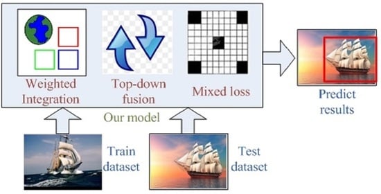
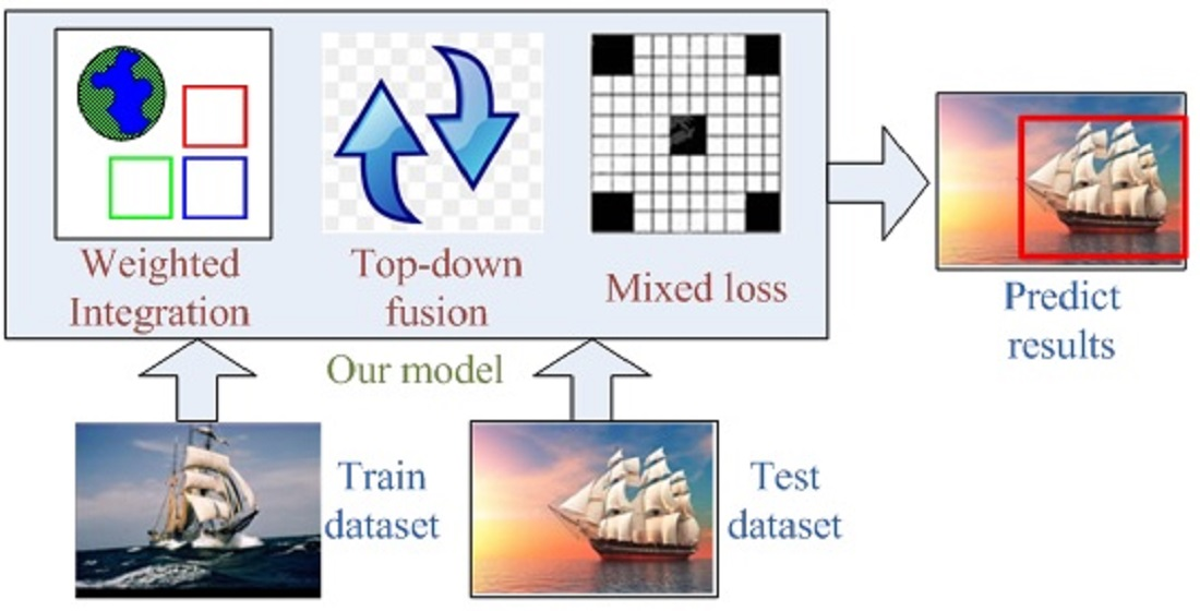
:Synthetic Aperture Radar (SAR), an active remote sensing imaging radar technology, has certain surface penetration ability and can work all day and in all weather conditions. It is widely applied in ship detection to quickly collect ship information on the ocean surface from SAR images. However, the ship SAR images are often blurred, have large noise interference, and contain more small targets, which pose challenges to popular one-stage detectors, such as the single-shot multi-box detector (SSD). We designed a novel network structure, a combinational fusion SSD (CF-SSD), based on the framework of the original SSD, to solve these problems. It mainly includes three blocks, namely a combinational fusion (CF) block, a global attention module (GAM), and a mixed loss function block, to significantly improve the detection accuracy of SAR images and remote sensing images and maintain a fast inference speed. The CF block equips every feature map with the ability to detect objects of all sizes at different levels and forms a consistent and powerful detection structure to learn more useful information for SAR features. The GAM block produces attention weights and considers the channel attention information of various scale feature information or cross-layer maps so that it can obtain better feature representations from the global perspective. The mixed loss function block can better learn the positions of the truth anchor boxes by considering corner and center coordinates simultaneously. CF-SSD can effectively extract and fuse the features, avoid the loss of small or blurred object information, and precisely locate the object position from SAR images. We conducted experiments on the SAR ship dataset SSDD, and achieved a 90.3% mAP and fast inference speed close to that of the original SSD. We also tested our model on the remote sensing dataset NWPU VHR-10 and the common dataset VOC2007. The experimental results indicate that our proposed model simultaneously achieves excellent detection performance and high efficiency.
1. Introduction
As an active remote sensing imaging radar technology, Synthetic Aperture Radar (SAR) remote sensing has a certain surface penetration ability and can work all day and in all weather conditions, which makes up for the shortcomings of optical remote sensing and infrared remote sensing. Therefore, SAR has been widely applied to disaster monitoring, environmental monitoring, resource exploration, mapping, and military fields. In ship detection, this technology can quickly collect ship information on the ocean surface, which is important for marine safety [1].
Popular state-of-the-art object detection algorithms are mainly divided into two categories: one-stage algorithms and two-stage algorithms [2,3,4,5]. At present, one-stage algorithms, such as the You Only Look Once (YOLO) series, fully convolutional one-stage object detection (FCOS), and single-shot multi-box detector (SSD) [6,7,8,9,10], with both efficiency and performance, have gained more favor in several real-world practical applications and industrial fields. However, unlike images in ordinary target detection tasks, the ship’s SAR images often have some special characteristics. The images are blurred, have large noise interference, and contain more small targets. Moreover, the scale of different objectives may vary greatly. The targets have almost no texture features, resulting in high similarity between some background entities and the target. Therefore, it is insufficient to deal with the ship’s SAR images by relying on an object detection structure such as the SSD, which is directly designed for ordinary images. It is generally believed that there are two obvious drawbacks of the original SSD. First, the feature representations are inadequate and rough for final precise locations. Multi-scale features are not fully utilized to generate enough information for blurry or small targets. Actually, the problem usually belongs to feature fusion methods. Second, the prior anchors are usually predefined roughly and do not exactly match those of actual training datasets. In this study, according to the characteristics of the SAR image, we designed a novel network structure named the combinational fusion single-shot multi-box detector (CF-SSD), based on the framework of the original SSD. Our main contributions are summarized as follows:
First, we designed a new feature fusion module named combinational fusion (CF). Unlike feature pyramid networks (FPNs), CF fuses different feature maps by up-sampling and down-sampling operations. It enables every feature map to detect objects of all sizes at different levels. Therefore, the feature maps with CF fusing can complement and support each other for every target size, forming a consistent and powerful detection structure to learn more useful information for SAR features. In addition, the fusion process is concise and efficient.
Second, we designed a cross-layer global attention module (GAM). Unlike other attention mechanisms, which consider a single layer or a feature map, it considers the channel attention information of different scale feature information or cross-layer maps. It can reinforce important information in a single feature map, distinguish the importance between feature maps at different scales, be performed before the existing feature fusion modules (e.g., FPN), and be executed independently.
Third, we designed a new loss function called mixed loss that considers the corner and center coordinates simultaneously. Compared with the original SSD, the new loss function can more accurately learn the positions of the truth anchor boxes with almost no additional computing consumption.
The rest of this paper is organized as follows. Section 2 introduces the related work. Section 3 introduces the structure details and the key parts of the CF-SSD. Section 4 describes the experiment and settings and provides different comparative results on ship detection experiments by using the CF-SSD and other models, and some resulting examples are analyzed. Section 5 summarizes the full text.
2. Related Work
Traditional SAR ship detection methods include constant false alarm rate (CFAR) and its varieties, which detect ship targets by modeling the statistical distribution of background clutter information [11]. This kind of method is prone to make false detections and miss true targets in some complex environments, and cannot ensure stable detection performance. Recently, the convolutional neural network has gradually become the mainstream method for object detection owing to its excellent ability to extract the texture and contour features of the original image. It has better adaptability and higher accuracy than those traditional object detection methods. Deep learning technology is also applied widely in remote sensing image processing [12,13].
In terms of popular one-stage object detection technology, the earliest detector was YOLO, which is based on the regression problem; since then, several improved versions, including YOLO2, YOLO3, and YOLO4, have been put forward. YOLO3 further integrates many successful tricks of other detectors, including multi-scale feature fusion and the residual block. The SSD is another influential and fast one-stage detector, which generates prediction boxes of different feature maps and finally merges these predictions. The deconvolutional single-shot detector (DSSD) [14], an improved variant of SSD, obtains a new feature map through the deconvolution operation on the original feature map, making full use of the shallow features and replacing the backbone network with the Resnet-101 [15]. It obtained better accuracy than SSD in the VOC2007 dataset [16] but lower frames per second (FPS), which is one of the most important evaluation indicators for the speed of the detector. Further, the rainbow single-shot detector (RSSD) [17] fuses the initial features by pooling and deconvolution operations, which have forward and reverse information at the same time. Its FPS is much higher than that of DSSD. RetinaNet [18] adopts FPN in its network structure and introduces a new loss function, Focal Loss, to solve the problem of imbalance in the positive and negative sample proportions. RefineDet [19] refines twice for anchors and combines the advantages of one-stage and two-stage detectors. Bidirectional pyramid networks (BPNs) [20] propose a bidirectional FPN structure to obtain a high-quality detector. There are several other interesting works based on SSD, such as feature fusion single-shot multi-box detector (FSSD) [21], RFBNet [22], SSADet [23], and F_SE_SSD [24]. Most of them utilize the careful design of feature information fusion modules.
There has also been a lot of research on ship detection in SAR images through deep learning technology. Chang [25] proposed an improved YOLOv2 for ship SAR image processing by merging some of the convolution layers to achieve faster detection. Jin [26] proposed a lightweight patch-to-pixel convolutional neural network for ship detection via PolSAR images. It utilized contextual semantic information at all scales, and all feature maps from the top down are combined to improve the final result. Wei [27] used the high-resolution detection network HR-SDNET to reduce the loss of ship feature information and improve the detection performance. Tang [28] introduced a noise-level classifier to derive and classify the noise level of SAR images and designed a target potential area extraction module to extract the complete region of potential objects. Chen [29] combined the separation attention module into YOLOv3 to improve the detection effect of remote sensing images. Cui [13] proposed the dense attention pyramid network to replace the traditional pyramid for SAR images. Zhao [30] proposed an attention receptive pyramid to enhance the relationships among nonlocal features and adjust the information of different feature maps. Finally, Yu [31] used a two-way convolution method to learn more feature information through fewer convolution layers and designed a multi-scale mapping output structure to make more effective use of feature information.
3. Approach
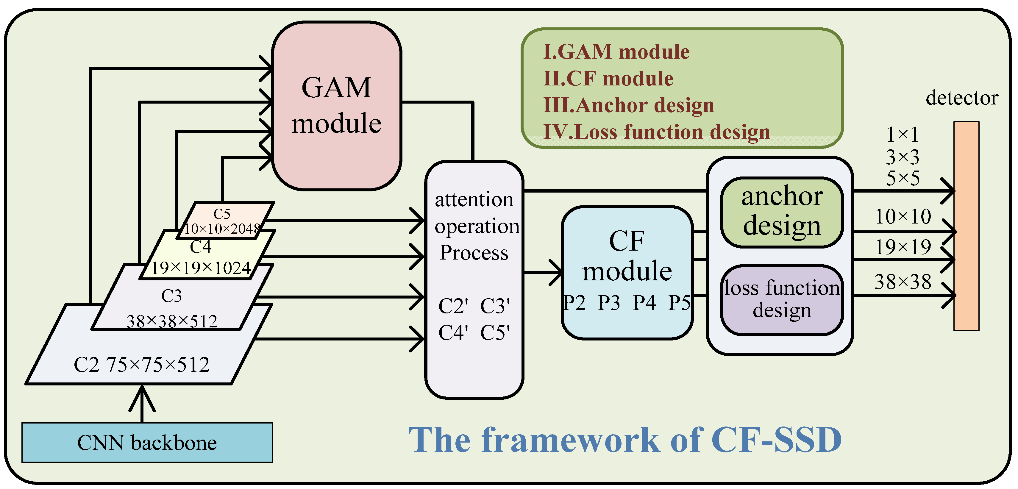
We propose a series of measures to solve the above problem of inadequate feature fusion of SSD-style one-stage object detectors. To verify the effectiveness of our proposed methods, we built a new detection model based on the SSD framework. Figure 1 shows an overview of our model, where the backbone network can be any deep neural network, such as VGG [32], ResNet, EfficientNet [33], MobileNet [34], CBResNet [35], or DenseNet [36]. In order to ensure fairness and impartiality in the comparison with other algorithms, we only used ResNet50 as the backbone network. As shown in Figure 1, after the proposed normalization preprocessing, input images are fed into the backbone network to generate four feature maps, C2, C3, C4, and C5. Then, the proposed GAM is plugged into the SSD framework. GAM takes C2, C3, C4, and C5 as input data and generates global channel weights for them. After integrating the four original feature maps with their own channel weights, new feature maps, C2’, C3’, C4’, and C5’, are obtained. Then, the CF process is triggered to merge multi-scale feature information and produce fused features P2, P3, P4, and P5. Finally, P5 creates four final feature maps with the sizes of 1 × 1, 3 × 3, 5 × 5, and 10 × 10 by continuous convolution operations. P2, P3, and P4 generate two final big feature maps with the scales 19 × 19 and 38 × 38, respectively. The model would be performed under the appropriate anchor design and loss function design. To show this more clearly, our works are illustrated in Figure 1, which shows four parts: the GAM, CF module, anchor design, and loss function design.
3.1. Global Attention Module
Many types of multi-scale feature fusion, such as FPN, realize the feature fusing layer-by-layer from the shallowest layer to the deepest layer of the CNN backbone. Many studies have enabled various improvements of feature fusion in object detection to further promote detection performance, including EFPN [37], DyFPN [38], and BPN [20]. Unlike those works, we were interested not in feature fusion but in the step before or after it. Therefore, we proposed a small block called GAM, containing the fusing channel information of all the feature maps. It can be plugged before any multi-scale feature fusion module.
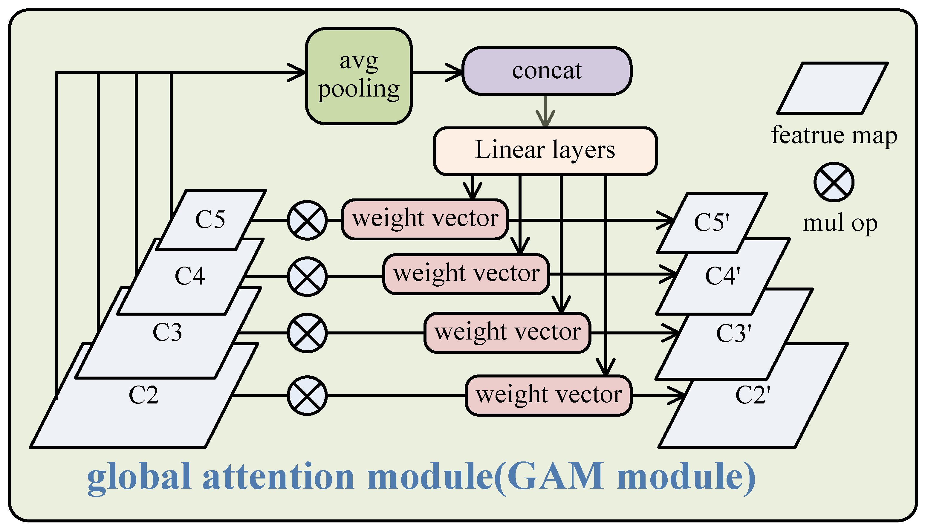
Typically, GAM takes a series of features generated from the backbone network {C2, C3, C4, C5} as input and then outputs the integrated features {C2′, C3′, C4′, and C5′}. The process is as follows, and is also shown in Figure 2:
where avgpool denotes the global average pooling operation, concat denotes the concatenation operation for multiple vectors, fc is the full connection layer, with sigmoid as its activation operator, ReLU is the rectified linear unit, and is the element-wise multiple operation on channel dimension. Traditionally, the channel attention mechanism is only implemented on each feature map, just as in SENet [39] or CBAM [40]. It obtains new feature maps with a stronger feature description by weighting the channels. The proposed GAM is different from these channel attention processes. GAM takes all the features into the full connection layer and outputs the weights of the channels of all the features. Therefore, the process is global-oriental, and the output weights can carry potential global information. In other words, these weights contain not only the important information of channels of individual maps but also the importance ratio between different feature maps. The reason for doing this is to make the next step, FPN or another multi-scale feature fusing module, more effective. By ignoring GAM, we need to perform feature fusion operations such as FPN directly on the multi-scale features {C2, C3, C4, C5} generated from the backbone network. For example, we will achieve new features {P2, P3, P4, P5} after FPN, and P2 can be seen as the fusion of multiple features:
Here, the multiple features are seen as equally weighted. Therefore, P2 cannot reflect the difference of importance between different feature maps. When GAM is added, the output features {C2′, C3′, C4′, C5′} carry the potential weights for different features. Therefore, P2 can be approximated as follows:
We consider that fusion feature P2 in Equation (6) should be better than that in Equation (5) for its additional information on the weights of different features. Through the GAM, both the channel attention and the feature attention are retained. By attaching the attention weights of multi-scale features, we think that the important detailed features from shallow layers are not easy to be covered by semantic information from deeper layers in the subsequent fusing process.
3.2. Combinational Fusion
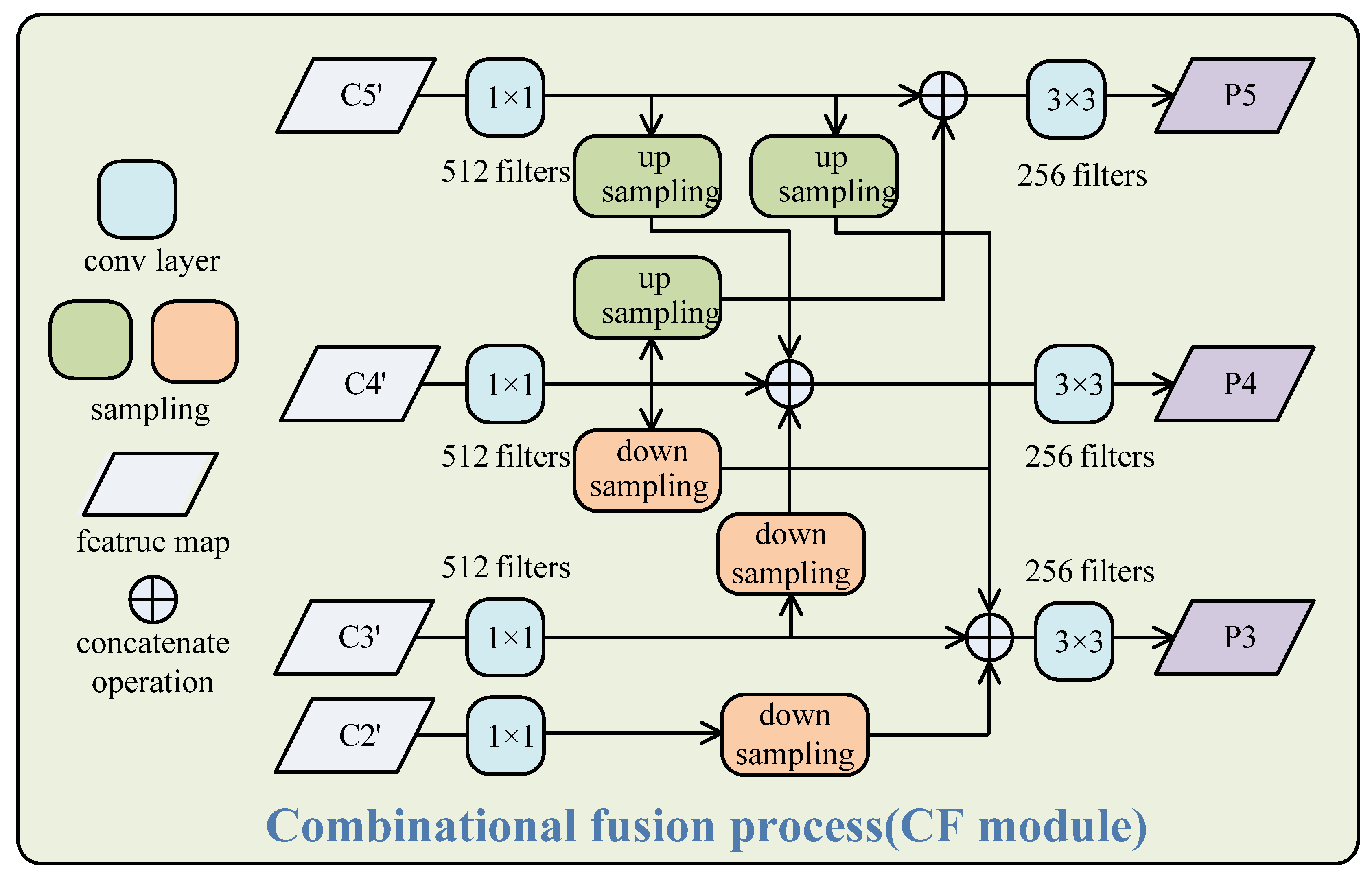
Here, we suggested a new feature fusion process called CF, as shown in Figure 3. It is unlike existing feature fusion methods, such as FPN, which walks a top-down fusion path from the deep layer to the shallow layer, or BiFPN [41], which contains two fusion steps with a top-down path and a bottom-up path, separately. The CF module also focuses on bi-directional fusion of feature maps from different layers, but it performs them at the same time. The features {C2′, C3′, C4′, C5′} from the GAM are taken as inputs of the CF module. They are first transformed into the same dimensions of 512 by 1 × 1 convolutional operations. Then, new features {P2, P3, P4, P5} are obtained through a series of sampling and combinational fusion processes, as in Equations (8)–(10). Here, the up-sampling and down-sampling processes adopt an interpolate operator with a ‘bilinear’ and 3 × 3 convolution operator with stride = 2, respectively. Finally, conv3 × 3 operations are performed for smoothing the fusion results.
The big maps from the shallow layers can locate the object well and preserve more details of targets, whereas the small maps from the deeper layers have a larger receptive field and can detect large and medium objects well. Therefore, P3 can recognize various targets better than C3′ and can detect small targets better than C4′ and C5′, the same as in FPN. However, it is not enough to rely on a single feature map, P3, for detecting small and occluded targets. Through combinational fusion, these feature maps can assist each other to detect targets of different scales. For example, P5 is mainly used to detect medium and large targets, but it can also provide some useful information for detecting small and occluded targets as a result of fusing C4′. P3 is mainly used to detect small and occluded targets, but it can also help detect large, fuzzy, and medium targets as a result of fusing C5′ and C4′. Note that the CF is performed in one step, which is different from the other bi-directional fusion methods with multi-step fusion, such as BiFPN and PAnet [42]; therefore, it is much more efficient and concise.
3.3. Reducing Convolution Computation
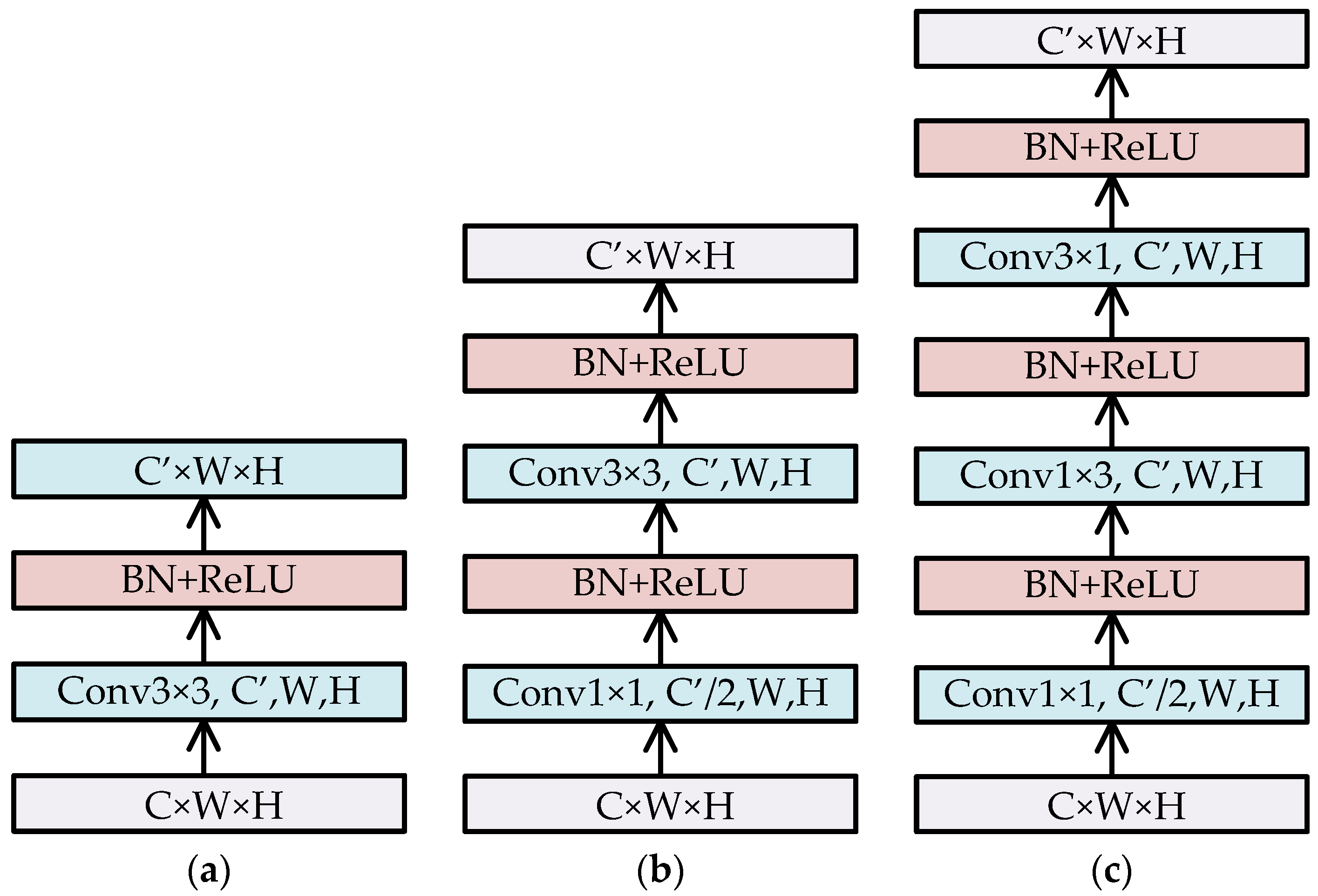
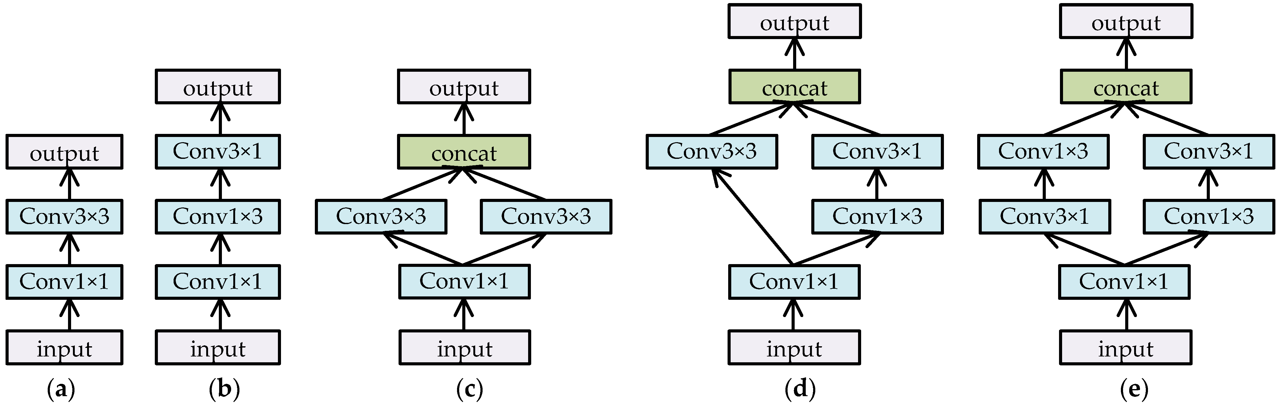
In the CF-SSD structure, it is inevitable to add several convolution operations, such as 3 × 3 convolution. These convolution operations will greatly increase the amount of computation and significantly reduce the inference speed. Therefore, we adopted bottleneck blocks similar to InceptionV2 [43] to modify some convolution operations. Figure 4 shows that how to transform feature maps with C × W × H into C′ × W × H by convolution operations. Scheme (a) uses the conv3 × 3 convolution operation directly, which produces about 9 × C × C′ × W × H multiplication operations. Scheme (b) first uses conv1 × 1 to reduce channels to half, and then uses conv3 × 3, which makes about 0.5 × C × C′ × W × H + 4.5 × C′ × C′ × W × H multiplication operations. When C ≥ C’, the convolution computation of (b) is less than about 55% of that of (a). Scheme (c) uses two asymmetric conv1 × 3 and conv3 × 1 to replace conv3 × 3 in (b); hence, it can achieve a computation cost that is lower than (b). We applied schemes (b) and (c) into Equation (11) of the CF module and used those convolution operations to produce feature maps with the sizes of 1 × 1, 3 × 3, and 5 × 5.
3.4. Anchor Design
In the original SSD, the size of the prior anchor of the feature map of layer i is defined as:
The default values of Smin and Smax are 0.2 and 0.9, respectively. From Equation (12), Sk ∈ {20, 37, 54, 71, 88}. For 300 × 300 input sizes, the prior anchor sizes of SSD are Sk ∈ {30, 60, 112, 162, 213, 264} and Sk+1 ∈ {60, 111, 162, 213, 264, 315}. The default prior anchor sizes are mainly suitable for some common detection datasets, such as the VOC dataset, but not for all the datasets, and this is because of the great variation in target sizes in different datasets. However, in the SSDD dataset, the small and medium targets account for a large proportion, and more than 70% of the object size is less than 20% of the original image size. The default prior anchors do not cover all the scales, thus making the speed and accuracy of training poorer. To avoid the mismatch between prior anchor sizes and target sizes, we set Smin and Smax as 0.1 and 0.5, respectively. The growth step, δ, of the feature maps is as follows:
Then, according to , Sk ∈ {10, 20, 30, 40, 50}. For 300 × 300 input sizes, the prior anchor sizes are Sk ∈ {15, 30, 60, 90, 120, 150} and Sk+1 ∈ {30, 60, 90, 120, 150, 180}. Table 1 shows that the adjusted prior box sizes will better match the SSDD dataset than the prior anchor of the original SSD. There are no default prior anchors of the original SSD to match those tiny object sizes of less than 1.0% of the scale of the image sizes, which should influence the training convergence speed and effect.
3.5. Normalization Parameter Setting
Usually, before being sent to the training model of detection, the input image needs to undergo normalization preprocessing. The normalization parameters, such as mean and SD, should be set in advance. We randomly sampled a part of images from the training set and then calculated the mean and SD of each channel. The values of mean and SD are used as normalization parameters for data normalization preprocessing. Owing to the randomness of sampling, the values will be slightly different each time, but the differences have little effect on the final result.
3.6. Mixed Loss Function Design
The loss function in this paper is shown in Equation (13). It is divided into three parts: position loss, Lloc, confidence loss, Lconf, and center position loss, Lloc_c. Lloc uses smoothL1 to calculate the error of coordinates between the real anchor and the predicted anchor, as in Equation (14). Lconf uses softmax loss to describe classification accuracy in Equation (16), which is similar to the SSD.
Here, c and p are the target class and the predicted confidence of the target class, respectively. l and g are the predicted position of the prior anchor and the position of ground truth, respectively. is an indicator function for class k, which equals 1 when the prior anchor i matches the ground truth j, and equals 0 otherwise. lx and ly, rx and ry, and cx and cy are the top-left, the bottom-right, and the center coordinates of the anchor, respectively.
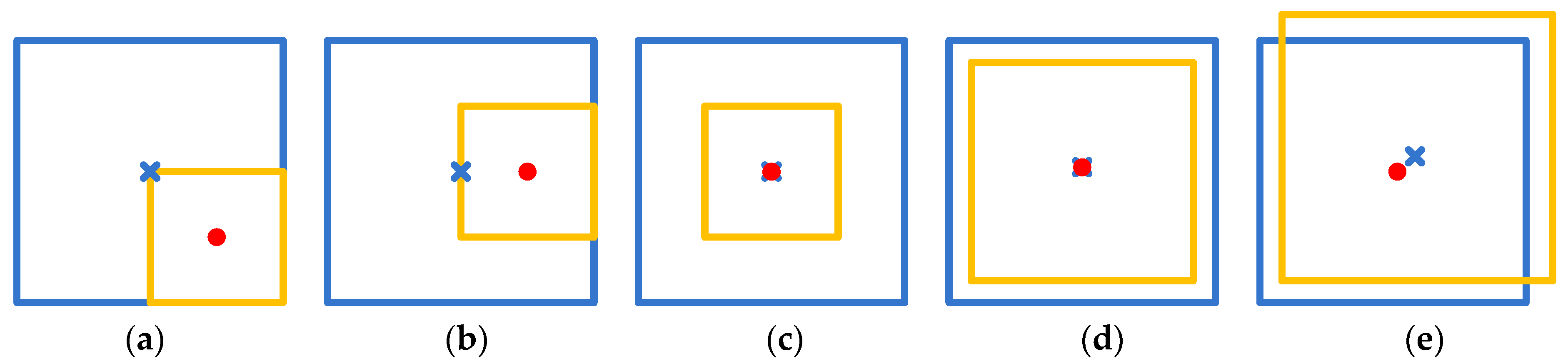
Lloc_c uses L2 loss to describe the error between the center coordinates of the real anchor and the predicted anchor, as in Equation (17). Lloc_c and Lloc together constitute the loss of the position and complement each other. As in Figure 5, the Lloc values of (a), (b), and (c) are probably the same; hence, the model cannot distinguish between them only by Lloc loss. However, their Lloc_c values are different, and the predicted anchor of (c) has the smallest loss by comparison, which is in line with our expectations. The Lloc definition of the original SSD includes the center coordinates and the width and height of the anchor. In Figure 5d,e, there are some deviations in the width and height in (d) and some deviations of the center coordinates in (e) between the real anchor and the predicted anchor. From the Lloc loss of the original SSD, they are probably the same, but (d) is always considered better in most cases. When using the proposed Lloc_c and Lloc definitions, (d) obtains a smaller loss value than that of (e), which is what we expect.
3.7. Training and Inference
Data augmentation: In order to provide our model with stronger generalization ability and to reduce the risk of over-fitting, there are preprocesses for the original training dataset before training, as follows: (1) normalization: this accelerates the convergence speed of gradient descent, (2) random flip: this flips the image randomly by a certain probability, (3) random expansion: this expands the image with the maximum expansion ratio of 4 and the RGB filling value, (4) random crop: this crops the image randomly to a certain size, and (5) random distortion: this performs random distortion on the image for brightness within the range [0.875, 1.125], contrast within the range [−0.5, 0.5], and saturation within the range [−0.5, 0.5].
CNN backbone architecture: We chose ResNet50 pre-trained on ImageNet as the backbone network in our experiments. For ensuring fairness in the experiment comparison, we use original ResNet50 as the backbone network, as in many other detectors. Therefore, in our model, the feature maps from the backbone network are directly generated from the original ResNet50 structure.
Optimization: For the SSDD dataset, we set the optimization parameters for 300 × 300 input size. Some training parameters vary for different datasets, such as max_iter and milestones. The training is completely fine-tuned for 30,000 iterations, with the batch size being 8. The base learning rate is set to 0.001 and then decreased to 0.0001 after 20,000 iterations. We used the stochastic gradient descent (SGD) method to optimize the model, with the value of momentum and weight decay being 0.9 and 0.0005, respectively. All the models were trained and optimized end-to-end. As we can see, these parameters are set with common values adopted in many existing related research works and have no bias against the proposed model.
Sampling balance: After anchor matching, the ratio of positive and negative anchors is imbalanced. The number of negative ones is much greater than that of the positive ones, which causes the effect of positive samples to become small in back propagation. We sampled a subset of negative anchors to keep the ratio of positive and negative ones as 1:3 for training, which is similar to that for the original SSD. The specific method is to select the part of negative anchors with the largest loss, which is three times the number of positive anchors.
Inference: After being obtained through the detector, the predicted boxes with a confidence under the threshold (e.g., 0.5) or belonging to the background are first filtered out. Then, we ranked them in descending order according to their confidence values, and only chose the top-k (e.g., 400) predicted boxes in the NMS step. Inference speed and performance are both our goals. Therefore, we hope that the inference speed of the proposed model is real-time and more than or at least close to the fastest speed of the SSD-style models.
4. Experiments
In our experiments, the performance of the proposed model was tested on two remote sensing object detection benchmarks that have been used in many prior studies: the SAR SSDD dataset [44] and the NWPUVHR-10 dataset [45]. The SSDD dataset contains 1160 SAR images and 2456 ships, with a 1–15 m resolution, as well as a format processed as the Pascal VOC 2007 dataset. There are ship targets in large sea areas and coastal areas, with 2.12 ships per image. NWPUVHR-10 is a 10-class geospatial object detection dataset, which contains 650 high-resolution remote sensing images manually annotated by experts, with each image containing at least one target to be recognized. These images were cropped from Google Earth, with spatial resolutions from 0.5 to 2.0 m, as well as the Vaihingen dataset, with a 0.08 m spatial resolution. For both the datasets, we selected 70% of the original images as the training set and 30% as the testing set. To ensure consistency of comparison, all models in the experiments used uniformly divided training and test sets.
The experiments were performed in a hardware environment with Intel i7 CPU and RTX Titan GPU. CUDA9.0 and cuDNN7.4 were used as the GPU acceleration library. The programming language used was Python3.7. The deep learning framework paddlepaddle (≥1.8 version) and paddleDetection toolboxes were selected to build the model. The original sizes of the image data in the experiment were different, but they were uniformly resized to 300 × 300 or 512 × 512 before being input to the model.
4.1. Evaluation Metrics
Following common practice, the evaluation metric of the experiments was the mean average precision (mAP), as in Equations (20)–(21), which was calculated from precision, p, and recall, r, where p denotes the proportion of positive samples in all the predicted positive ones, and r denotes the proportion of the samples that are both positive and predicted to be positive in all the positive samples. K is the number of categories.
Here, TP is true positive, FP is false positive, and FN is false negative. In this test, if the Intersection Over Union (IOU) between the prediction area and ground truth area was higher than 0.5, it was defined as TP. If the IOU was lower than 0.5, it was defined as FP. The actual target that was not detected was defined as FN.
4.2. Comparative Experiment
4.2.1. Test on VOC2007 Dataset
To verify the validity and generalization of the model, we used the Pascal VOC2007 dataset to validate the model’s ability to detect on common datasets. Table 2 presents the experimental results of classical architectures, some recent state-of-the-art detectors, and our CF-SSD on the VOC2007 test. Under a small input size of 300 × 300, CF-SSD achieved 80.9% mAP, with a ResNet50 backbone and a fast inference speed. It outperformed most one-stage detectors shown in Table 2, such as RSSD300, DSSD320, RefineDet320, BPN320, and RFBNet300. In addition, Table 2 includes some recent two-stage detectors based on the ResNet101 backbone and 600 × 1000 input size, such as R-FCN, R-FCN Cascade, and CoupleNet. Our model obtained excellent Map results under the 300 × 300 input size, exceeding most other models in Table 2. Although a few models such as Cascade R-CNN achieve higher precision than our model, they have larger input size and run slower. Therefore, CF-SSD achieved almost excellent results of accuracy and efficiency, simultaneously.
4.2.2. Test on SSDD Dataset
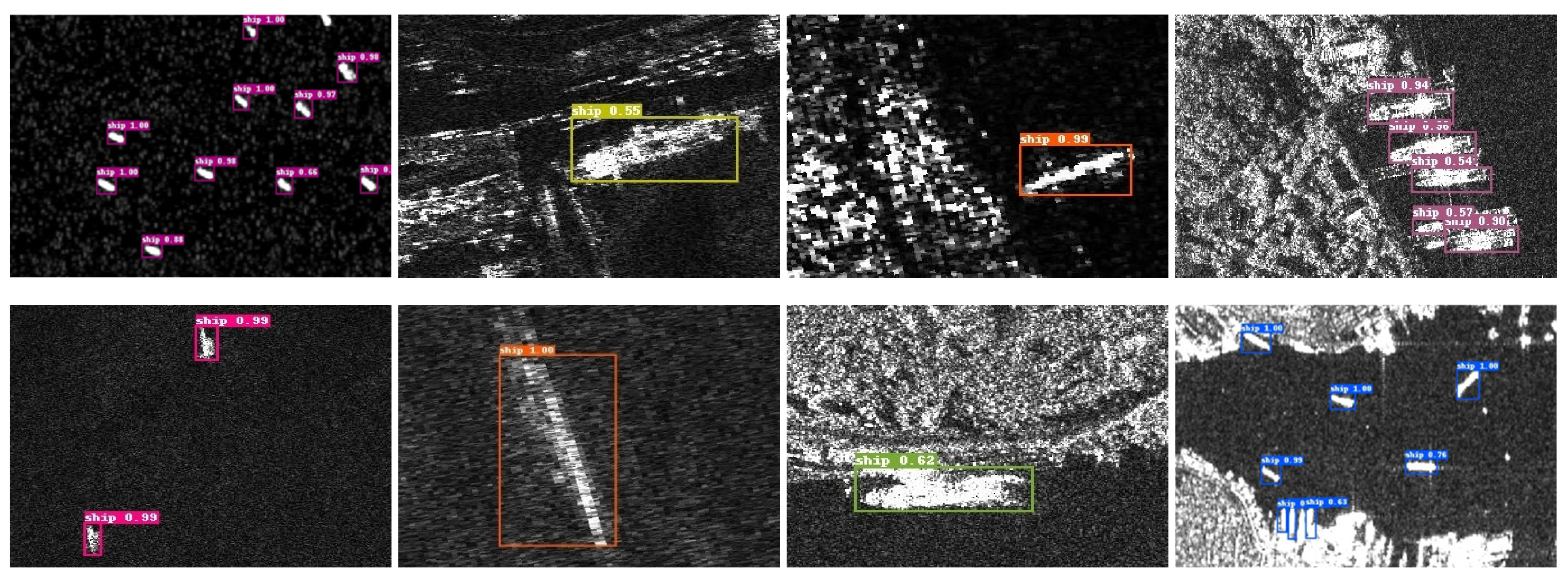
The SSDD dataset is one of the main test datasets. Some data are shown in Figure 6, which shows small ship targets in large sea areas, blurred ship objects, ship targets in coastal areas, and ship targets in some complex background similar to themselves. Detection in these images poses challenges in accurately identifying ship targets.
Ablation study: We performed a series of ablation experiments on the SSDD dataset to observe the effect of different components of CF-SSD, as shown in Table 3. We built the baseline model inspired by the SSD with the pre-trained backbone VGG16. The original SSD in Table 3 denotes the SSD with the default prior anchors, and the SSD denotes the SSD with the revised prior anchors, as in Section 3.4. On adding the CF and adjusting the anchor setting, the SSD + CF model achieved a significant improvement over the baseline SSD. Of course, when combining CF, mixed loss, and GAM, the best result was obtained. In contrast, the contribution of GAM was relatively small. In addition, we replaced GAM with the Squeeze-and-Excitation (SE) [39] block and the Spatial Attention (SA) [40] block to observe the effects of the two blocks. The SE block is a channel attention mechanism for acquiring channel weights, and the SA block is a spatial attention mechanism from CBAM for acquiring pixel weights. The last two rows of Table 3 illustrate that neither of them could effectively improve the model based on CF and mixed loss.
Reducing convolution computationtest: In Section 3.3, we presented a few structures, such as those shown in Figure 4b,c, to replace the conv3 × 3 operations in order to effectively decrease the computational cost. In fact, several other structures were also tested in our experiments to verify their effects and efficiency, as shown in Figure 7. Figure 7c–e shows two branches with convolution operations and concatenates them as outputs so as to extract more meaningful features by multi-way paths. However, through some experiments, we found that there was little difference in their final accuracy results and inference speeds. Figure 7c–e does not show any advantages over Figure 7a,b. Therefore, there is no need to list the comparison results here. It is worth mentioning that compared to the simple scheme shown in Figure 4a, the structures shown in Figure 7 were all obviously superior in inference efficiency.
Comparative experiment: Table 4 presents the experimental results of recent excellent detectors and our CF-SSD on the SSDD dataset, with small input sizes such as 300 × 300 or 384 × 384. The models include some improved detectors based on SSD, such as RetinaNet, anchor-free detectors such as FCOS, and some other famous models. For comparative fairness, these models only use two backbones: ResNet50 or VGG16. Although the experimental results fluctuate slightly, CF-SSD achieved a better mAP result and inference precision than most other detectors. In our experiments, YOLO and FCOS detectors also achieved excellent mAP values. The fourth column of Table 4 shows the inference speeds of CF-SSD and the other detectors. CF-SSD with the ResNet50 backbone also did well to obtain a higher FPS, indicating that it is fully satisfactory for many real-time applications. The CF-SSD was not the fastest detector, but considering the inference accuracy and inference efficiency simultaneously, it achieved excellent tradeoffs. Particularly, compared to the variants of the SSD, CF-SSD was superior.
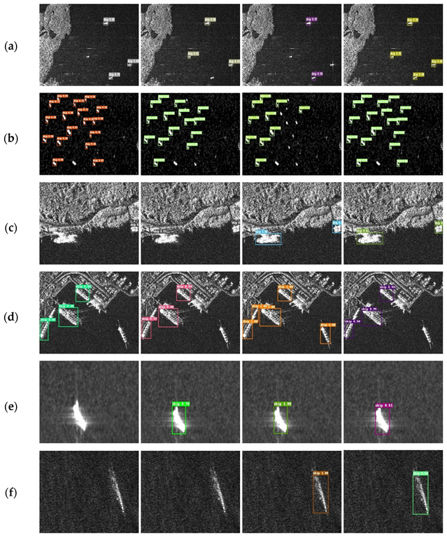
Visualization evaluation: Figure 8 shows the visual detection results of some different detection methods with SSD, SSD+FPN, RetinaNet480, and CF-SSD. It can be seen from the diagram that (a, b) small target in large sea area, (c, d) complex background near the shore, and (e, f) blurred ship target are common samples, which are also difficult points in SAR ship detection. The high noise signals and blurred pixels of SAR images made small target detection more difficult. Near-shore targets are often close to the shore; hence, their detection could easily be disturbed by a complex background. The figure shows that SSD performed poorly in the detection of small targets and near-shore targets, SSD+FPN missed some blurred ship targets, and RetinaNet did not do well enough on small target detection and made some false detection. RetinaNet showed some advantages in some difficult targets, as shown in Figure 8d, and the SSD inferred faster than the others. Considering all the aspects, CF-SSD had a better comprehensive performance.
4.2.3. Test on NWPUVHR-10 Dataset
We also conducted experiments on the NWPUVHR-10 dataset to verify the validity and generalization of CF-SSD. The NWPUVHR-10 dataset contains 10 classes of objects: airplane, ship, ST, BD, TC, BC, GFT, harbor, bridge, and vehicle. The dataset contains many small and medium targets, and shows different scales of objectives. There are similarities between some background units and targets in texture or shape. The most optimization parameters of the experiments for NWPUVHR-10 were in the SSDD dataset. Particularly, the base learning rate was 0.001 for the first 200 epochs, with 300 warmup steps and decays to 0.0001 for the latter 50 epochs.
Comparative experiment: Table 5 presents the experimental results of some recent state-of-the-art detectors and our CF-SSD on the NWPUVHR-10 dataset, with big input sizes such as 512 × 512 or 600 × 1000. Most results are cited from published literature, while the others are our experimental results. The compared models included Faster RCNN, R-FCN, Multi-scale CNN, RetinaNet, and YOLOv3. CF-SSD achieved 90.6% mAP, superior to any detector listed in Table 5, and with a fast inference speed.
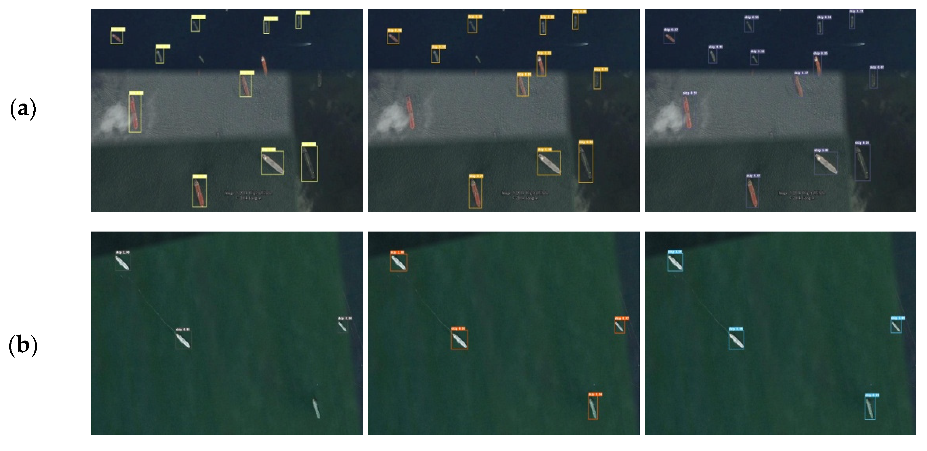
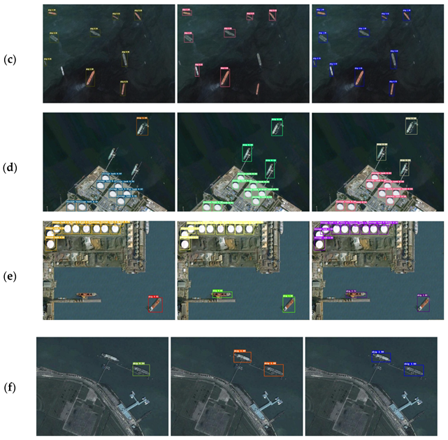
Visualization evaluation: We conducted a qualitative comparison of CF-SSD, SSD+FPN, and SSD with input size 512 × 512 on the ship objects of NWPUVHR-10 dataset. Figure 9 shows some examples of their detection outputs. In Figure 9a–c, it is clear that in the background of the empty ocean, SSD512 and SSD+FPN missed some offshore small ship targets. SSD+FPN sometimes may even miss some not-so-small targets, as shown in Figure 9a, which reflects its instability. Moreover, Figure 9d–f show that with SSD512, it is easy to miss those docked ships due to interference from nearside background units. In contrast, CF-SSD512 may have detected these targets more easily than the others. We think that because different weights for multi-scale features are lacking, some important detailed features are not covered by semantics from deeper layers in FPN fusing. Furthermore, the more detailed information cross-layers in CF also help us to tackle small or fuzzy objects. These factors may make CF-SSD512 more effective and comprehensive, with a stronger interference resistance and higher accuracy.
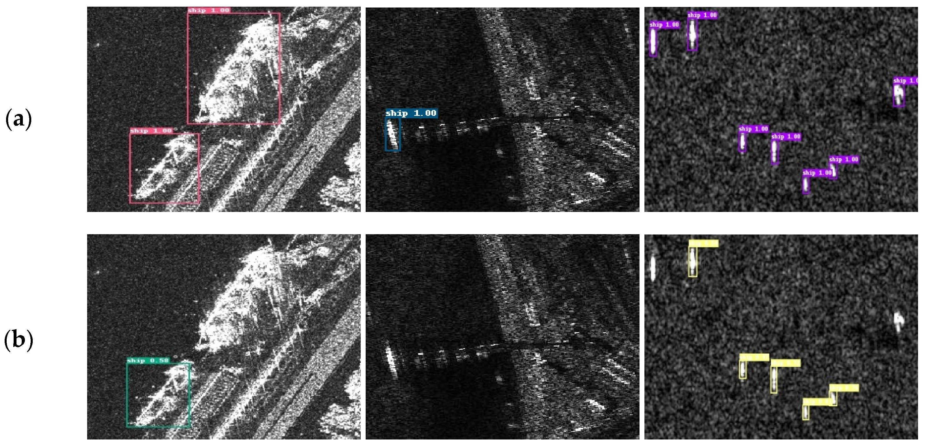
4.3. Error Analysis and Discussion
Although the proposed CF-SSD improved the detection accuracy, it still caused some errors and missing cases. Figure 10 shows some failed detection samples. As shown in the first and second columns of Figure 10, some objects with high noise and complex background were missed. This noise was inherent in SAR itself. In the radar echo signals, the gray values of adjacent pixels would fluctuate randomly within a certain range for their coherence. The noise may make some background units similar to the targets, making the detection even harder. The CF-SSD needs to strengthen its capacity to tackle this problem.
As in the third column of Figure 10, some small or blurry objects were missed. The problems are difficult to solve perfectly owing to the limited resolution of input features. One straightforward and possibly effective approach is to employ larger feature maps with more information to perform detection, as in some recent research. For example, we may add a feature map with 75 × 75 size into SSD300 to improve the capability of small object detection, whereas the largest feature size of the original SSD300 is only 38 × 38. However, this method will significantly increase computational complexity, training cost, and inference cost. In addition, the experimental comparisons were also unfair under different sizes of input features for different algorithms. Therefore, in this paper, we only used the same feature sizes consistent with the original SSD and many other one-stage models. In general, the focus of these difficult cases is still on how to extract more effective features of the limited-resolution inputs and on how to define a more appropriate loss function, which we plan to examine in our future work.
5. Conclusions
Ship detection of SAR images is a challenging task due to fuzzy images, sparse objects, and strong noise interference. In this paper, we presented a novel single-shot one-stage detector, the CF-SSD, for SAR ship detection, which tries to utilize GAM, CF, and mixed loss to achieve better performance. To consider the importance of different feature maps derived from the backbone, which is convenient for subsequent layer fusing, the GAM integrating cross-layer channel attention was proposed. To further improve the fusion effect, we proposed the CF module by fusing the combination and crossover layers to ensure that each feature map has more target information. To more accurately locate the prediction anchor, we proposed the mixed loss instead of the original SSD loss to describe the prediction deviation more comprehensively. The experimental results show that compared with other models, our model achieved better tradeoffs between detection performance and inference speed. In addition, although the three modules are used in the SSD framework in the paper, they can also be embedded in other detection frameworks and can be used individually. The CF module expresses a new way of integrating feature maps. The GAM indicates a modification of the SE module from a global perspective. Mixed loss acts as a supplement to the original SSD loss.
In our future work, our model will include the following aspects for further research and improvement: (1) a special module for anchor refinement, such as the region proposal network (RPN) [4], which can roughly correct the position of the anchor, (2) a better loss function that considers hard examples of mining, and (3) a model structure that can extract more effective features of blurred and tiny objects from SAR images.
Author Contributions
Conceptualization, methodology, formal analysis, L.X. and C.P.; writing—original draft preparation, experiment, project administration, L.X.; validation, writing—review and editing, C.P.; resources, data curation, experiment, supervision, Y.G. and Z.S. All authors have read and agreed to the published version of the manuscript.
Funding
This research was funded by the Science and Technology innovation 2025 major special project of Ningbo of China, grant number 2019B10036, and the Natural Science Foundation of China, grant numbers 61872321 and 62172356.
Data Availability Statement
Publicly available datasets were used in this study. SSDD data can be found at: https://pan.baidu.com/share/init?surl=E8ixqK5AVfXc98UgQmpqaw, accessed on 21 October 2021. The extraction code is trnt, and the decompression password is 12345qwert. NWPUVHR-10 data can be found at: https://pan.baidu.com/s/1Wm73acTD1WfBM_YZlKMjXw, accessed on 21 October 2021. The extraction code is 35wf.
Acknowledgments
The authors would like to thank the editors and the reviewers for their valuable suggestions.
Conflicts of Interest
The authors declare no conflict of interest.
Abbreviations
The following abbreviations are used in this manuscript:
| CF-SSD | Combinational Fusion Shot Multi-box Detector |
| GAM | Global Attention Module |
| CF | Combinational Fusion |
| SAR | Synthetic Aperture Radar |
| FCOS | Fully Convolutional One-Stage Object Detection |
| YOLO | You Only Look Once |
| SSD | Single-Shot Multi-Box Detector |
| CNN | Convolutional Neural Network |
| FPN | Feature Pyramid Network |
| R-CNN | Regions with CNN Features |
| DSSD | Deconvolutional Single-Shot Detector |
| RSSD | Rainbow Single-Shot Detector |
| FSSD | Feature Fusion Single-Shot Multi-box Detector |
| FMSSD | Feature-Merged Single-Shot Detector |
| FCN | Fully Convolution Network |
| ION | Inside-Outside Net |
| PANet | Path Aggregation Network |
| BPN | Bidirectional Pyramid Network |
| BiFPN | Bidirectional Feature Pyramid Network |
| EFPN | Extended Feature Pyramid Network |
| CBAM | Convolutional Block Attention Module |
| SE | Squeeze and Excitation |
| RPN | Region Proposal Network |
| FPS | Frames Per Second |
| ReLU | Rectified Linear Unit |
| BN | Batch Normalization |
| IOU | Intersection Over Union |
| TP | True Positive |
| FP | False Positive |
| FN | False Negative |
| NMS | Non-Maximum Suppression |
| SGD | Stochastic Gradient Descent |
| GPU | Graphics Processing Unit |
| RPN | Region Proposal Network |
References
- Liu, W.; Ma, L.; Chen, H. Arbitrary-Oriented Ship Detection Framework in Optical Remote-Sensing Images. IEEE Geosci. Remote Sens. Lett. 2018, 15, 937–941. [Google Scholar] [CrossRef]
- Cai, Z.; Vasconcelos, N. Cascade r-cnn: Delving into high quality object detection. In Proceedings of the 2018 IEEE/CVF Conference on Computer Vision and Pattern Recognition, Salt Lake City, UT, USA, 18–23 June 2018. [Google Scholar]
- He, K.; Gkioxari, G.; Dollar, P.; Girshick, R. Mask r-cnn. In Proceedings of the 2017 IEEE International conference on Computer vision (ICCV), Venice, Italy, 22–29 October 2017; pp. 2980–2988. [Google Scholar]
- Ren, S.; He, K.; Girshick, R.; Sun, J. Faster r-cnn: Towards realtime object detection with region proposal networks. IEEE Trans. Pattern Anal. Mach. Intell. 2017, 6, 1137–1149. [Google Scholar] [CrossRef] [Green Version]
- Bell, S.; Lawrence, C.Z.; Bala, K.; Girshick, R. Inside-outside net: Detecting objects in context with skip pooling and recurrent neural networks. In Proceedings of the IEEE Conference on Computer Vision and Pattern Recognition, Las Vegas, NV, USA, 26 June–1 July 2016; pp. 2874–2883. [Google Scholar]
- Redmon, J.; Divvala, S.; Girshick, R.; Farhadi, A. You only look once: Unified, real-time object detection. In Proceedings of the IEEE Conference on Computer Vision and Pattern Recognition (CVPR), Las Vegas, NV, USA, 26 June–1 July 2016. [Google Scholar]
- Redmon, J.; Farhadi, A. Yolo9000: Better, faster, stronger. In Proceedings of the 2017 IEEE Conference on Computer Vision and Pattern Recognition (CVPR), Honolulu, HI, USA, 21–26 July 2017. [Google Scholar]
- Redmon, J.; Farhadi, A. Yolov3: An incremental improvement. arXiv 2018, arXiv:1804.02767. [Google Scholar]
- Liu, W.; Anguelov, D.; Erhan, D.; Szegedy, C.; Reed, S.; Fu, C.; Berg, A. SSD: Single shot multibox detector. In Proceedings of the European Conference on Computer Vision, Amsterdam, The Netherlands, 8–16 October 2016. [Google Scholar]
- Tian, Z.; Shen, C.; Chen, H.; He, T. Fcos: Fully convolutional one-stage object detection. In Proceedings of the IEEE International Conference on Computer Vision, Seoul, Korea, 27 October–2 November 2019; pp. 9627–9636. [Google Scholar]
- Xianxiang, Q.; Shilin, Z.; Huanxin, Z.; Gui, G. A CFAR Detection Algorithm for Generalized Gamma Distributed Background in High-Resolution SAR Images. IEEE Geosci. Remote Sens. Lett. 2013, 10, 806–810. [Google Scholar] [CrossRef]
- Yin, W.; Diao, W.; Wang, P.; Gao, X.; Li, Y.; Sun, X. PCAN—Part-Based Context Attention Network for Thermal Power Plant Detection in Remote Sensing Imagery. Remote Sens. 2021, 13, 1243. [Google Scholar] [CrossRef]
- Cui, Z.; Li, Q.; Cao, Z.; Liu, N. Dense Attention Pyramid Networks for Multi-Scale Ship Detection in SAR Images. IEEE Trans. Geosci. Remote Sens. 2019, 57, 8983–8997. [Google Scholar] [CrossRef]
- Fu, C.; Liu, W.; Ranga, A.; Tyagi, A.; Berg, A.C. DSSD: Deconvolutional single shot detector. arXiv 2017, arXiv:1701.06659. [Google Scholar]
- He, K.; Zhang, X.; Ren, S.; Sun, J. Deep residual learning for image recognition. In Proceedings of the IEEE Conference on Computer Vision and Pattern Recognition (CVPR), Las Vegas, NV, USA, 26 June–1 July 2016; pp. 770–778. [Google Scholar]
- Everingham, M.; Van Gool, L.; Williams, C.; Winn, J.; Zisserman, A. The pascal visual object classes (voc) challenge. Int. J. Comput. Vis. 2010, 88, 303–338. [Google Scholar] [CrossRef] [Green Version]
- Jeong, J.; Park, H.; Kwak, N. Enhancement of SSD by concatenating feature maps for object detection. arXiv 2017, arXiv:1705.09587. [Google Scholar]
- Tsung, Y.L.; Goyal, P.; Girshick, R.; He, K.; Dollar, P. Focal Loss for Dense Object Detection. IEEE Trans. Pattern Anal. Mach. Intell. 2017, 99, 2999–3007. [Google Scholar]
- Zhang, S.; Wen, L.; Bian, X.; Lei, Z.; Li, S.Z. Single-shot refinement neural network for object detection. In Proceedings of the IEEE Conference on Computer Vision and Pattern Recognition, Salt Lake City, UT, USA, 18–23 June 2018; pp. 4203–4212. [Google Scholar]
- Wu, X.; Zhang, D.; Zhu, J.; Hoi, S.C.H. Single-Shot Bidirectional Pyramid Networks for High-Quality Object Detection. Neurocomputing 2020, 401, 1–9. [Google Scholar] [CrossRef] [Green Version]
- Li, Z.; Zhou, F. FSSD: Feature Fusion Single Shot Multibox Detector. arXiv 2017, arXiv:1712.00960. [Google Scholar]
- Liu, S.; Di, H.; Wang, Y. Receptive Field Block Net for Accurate and Fast Object Detection. In Proceedings of the IEEE Conference on Computer Vision and Pattern Recognition, Salt Lake City, UT, USA, 18–23 June 2018. [Google Scholar]
- Leng, J.; Liu, Y. Single-shot augmentation detector for object detection. Neural Comput. Appl. 2020, 33, 3583–3596. [Google Scholar] [CrossRef]
- Zheng, P.; Bai, H.Y.; Li, W.; Guo, H.W. Small target detection algorithm in complex background. J. Zhejiang Univ. Eng. Sci. 2020, 54, 1–8. [Google Scholar]
- Chang, Y.-L.; Anagaw, A.; Chang, L.; Wang, Y.; Hsiao, C.-Y.; Lee, W.-H. Ship Detection Based on YOLOv2 for SAR Imagery. Remote Sens. 2019, 11, 786. [Google Scholar] [CrossRef] [Green Version]
- Jin, K.; Chen, Y.; Xu, B.; Yin, J.; Wang, X.; Yang, J. A Patch-to-Pixel Convolutional Neural Network for Small Ship Detection with PolSAR Images. IEEE Trans. Geosci. Remote Sens. 2020, 58, 6623–6638. [Google Scholar] [CrossRef]
- Wei, S.; Su, H.; Ming, J.; Wang, C.; Yan, M.; Kumar, D.; Shi, J.; Zhang, X. Precise and Robust Ship Detection for High-Resolution SAR Imagery Based on HR-SDNet. Remote Sens. 2020, 12, 167. [Google Scholar] [CrossRef] [Green Version]
- Tang, G.; Zhuge, Y.; Claramunt, C.; Men, S. N-YOLO: A SAR Ship Detection Using Noise-Classifying and Complete-Target Extraction. Remote Sens. 2021, 13, 871. [Google Scholar] [CrossRef]
- Chen, L.; Shi, W.; Deng, D. Improved YOLOv3 Based on Attention Mechanism for Fast and Accurate Ship Detection in Optical Remote Sensing Images. Remote Sens. 2021, 13, 660. [Google Scholar] [CrossRef]
- Zhao, Y.; Zhao, L.; Xiong, B.; Kuang, G. Attention Receptive Pyramid Network for Ship Detection in SAR Images. IEEE J. Sel. Top. Appl. Earth Obs. Remote Sens. 2020, 13, 2738–2756. [Google Scholar] [CrossRef]
- Yu, L.; Wu, H.; Zhong, Z.; Zheng, L.; Deng, Q.; Hu, H. TWC-Net: A SAR Ship Detection Using Two-Way Convolution and Multiscale Feature Mapping. Remote Sens. 2021, 13, 2558. [Google Scholar] [CrossRef]
- Simonyan, K.; Zisserman, A. Very deep convolutional networks for large-scale image recognition. arXiv 2014, arXiv:1409.1556. [Google Scholar]
- Tan, M.; Le, Q.V. EfficientNet: Rethinking Model Scaling for Convolutional Neural Networks. In Proceedings of the International Conference on Machine Learning, Long Beach, CA, USA, 10–15 June 2019. [Google Scholar]
- Sandler, M.; Howard, A.; Zhu, M.; Zhmoginov, A.; Chen, L.C. MobileNetV2: Inverted Residuals and Linear Bottlenecks. In Proceedings of the IEEE Conference on Computer Vision and Pattern Recognition (CVPR), Salt Lake City, UT, USA, 18–23 June 2018. [Google Scholar]
- Liu, Y.; Wang, Y.; Wang, S.; Liang, T.; Zhou, Q.; Tang, Z.; Ling, H. CBNet: A Novel Composite Backbone Network Architecture for Object Detection. arXiv 2019, arXiv:1909.03625. [Google Scholar] [CrossRef]
- Iandola, F.; Moskewicz, M.; Karayev, S.; Girshick, R.; Darrell, T.; Keutzer, K. Densenet: Implementing efficient convnet descriptor pyramids. arXiv 2014, arXiv:1404.1869. [Google Scholar]
- Deng, C.; Wang, M.; Liu, L.; Liu, Y. Extended Feature Pyramid Network for Small Object Detection. In Proceedings of the IEEE Conference on Computer Vision and Pattern Recognition (CVPR), Seattle, WA, USA, 14–19 June 2020. [Google Scholar]
- Zhu, M.; Han, K.; Yu, C.; Wang, Y. Dynamic Feature Pyramid Networks for Object Detection. arXiv 2020, arXiv:1612.03144. [Google Scholar]
- Hu, J.; Shen, L.; Albanie, S.; Sun, G.; Wu, E. Squeeze-and-Excitation Networks. In Proceedings of the IEEE Conference on Computer Vision and Pattern Recognition (CVPR), Salt Lake City, UT, USA, 18–23 June 2018; pp. 7132–7141. [Google Scholar]
- Woo, S.; Park, J.; Lee, J.Y.; Kweon, I.S. CBAM: Convolutional Block Attention Module. In Proceedings of the European Conference on Computer Vision, Munich, Germany, 8–14 September 2018. [Google Scholar]
- Tan, M.; Pang, R.; Le, Q.V. EfficientDet: Scalable and Efficient Object Detection. In Proceedings of the IEEE Conference on Computer Vision and Pattern Recognition (CVPR), Seattle, WA, USA, 14–19 June 2020. [Google Scholar]
- Liu, S.; Qi, L.; Qin, H.; Shi, J.; Jia, J. Path Aggregation Network for Instance Segmentation. In Proceedings of the IEEE Conference on Computer Vision and Pattern Recognition (CVPR), Salt Lake City, UT, USA, 18–23 June 2018. [Google Scholar]
- Szegedy, C.; Vanhoucke, V.; Ioffe, S.; Shlens, J.; Wojna, Z. Rethinking the Inception Architecture for Computer Vision. In Proceedings of the 2016 IEEE Conference on Computer Vision and Pattern Recognition (CVPR), Las Vegas, NV, USA, 26 June–1 July 2016; pp. 2818–2826. [Google Scholar]
- Li, J.; Qu, C.; Shao, J. Ship detection in SAR images based on an improved faster R-CNN. In Proceedings of the 2017 SAR in Big Data Era: Models, Methods and Applications (BIGSARDATA), Beijing, China, 13–14 November 2017; pp. 1–6. [Google Scholar]
- NWPU VHR-10 Dataset. Available online: http://www.escience.cn/people/gongcheng/NWPU-VHR-10.html (accessed on 21 October 2021).
- Dai, J.; Li, Y.; He, K.; Sun, J. R-FCN: Object Detection via Region-based Fully Convolutional Networks. In Proceedings of the 30th Conference on Neural Information Processing Systems, Barcelona, Spain, 5–8 December 2016. [Google Scholar]
- Zhu, Y.; Zhao, C.; Wang, J.; Zhao, X.; Wu, Y.; Lu, H. Couplenet: Coupling global structure with local parts for object detection. In Proceedings of the IEEE international conference on computer vision, Venice, Italy, 22–29 October 2017; pp. 4126–4134. [Google Scholar]
- Liu Wang, X.L. Single-stage object detection using filter pyramid and atrous convolution. J. Image Graph. 2020, 25, 0102–0112. [Google Scholar]
- Han, X.; Zhong, Y.; Zhang, L. An efficient and robust integrated geospatial object detection framework for high spatial res-olution remote sensing imagery. Remote Sens. 2017, 9, 666. [Google Scholar] [CrossRef] [Green Version]
- Xu, Z.; Xin, X.; Wang, L.; Yang, R.; Pu, F. Deformable convnet with aspect ratio constrained NMS for object detection in remote sensing imagery. Remote Sens. 2017, 9, 1312. [Google Scholar] [CrossRef] [Green Version]
- Ren, Y.; Zhu, C.; Xiao, S. Deformable faster R-CNN with aggregating multi-layer features for partially occluded object detection in optical remote sensing images. Remote Sens. 2018, 10, 1470. [Google Scholar] [CrossRef] [Green Version]
- Chen, S.; Zhan, R.; Zhang, J. Geospatial object detection in remote sensing imagery based on multiscale single-shot detector with activated semantics. Remote Sens. 2018, 10, 820. [Google Scholar] [CrossRef] [Green Version]
- Guo, W.; Yang, W.; Zhang, H.; Hua, G. Geospatial object detection in high resolution satellite images based on multi-scale convolutional neural network. Remote Sens. 2018, 10, 131. [Google Scholar] [CrossRef] [Green Version]
- Wang, P.; Sun, X.; Diao, W.; Fu, K. FMSSD: Feature-Merged Single-Shot Detection for Multiscale Objects in Large-Scale Remote Sensing Imagery. IEEE Trans. Geosci. Remote Sens. 2020, 58, 3377–3390. [Google Scholar] [CrossRef]
Figure 1.
The proposed framework of the CF-SSD. The input image is normalized first and then sent to the backbone network to produce four basic feature maps. Then, the feature maps are converted into new features by the GAM and CF modules. Our work comprises (I) GAM, (II) CF, (III) anchor design, and (IV) loss function design.

Figure 2.
The structure of GAM. The inputs from the backbone are concatenated into a vector after 1 × 1 convolution operations and average pooling operations. Then, through linear layers, the weight vectors for every channel of every feature map are obtained.
Figure 2.
The structure of GAM. The inputs from the backbone are concatenated into a vector after 1 × 1 convolution operations and average pooling operations. Then, through linear layers, the weight vectors for every channel of every feature map are obtained.

Figure 3.
The structure of the CF module. The feature maps from the GAM pass through 1 × 1 convolution to the same dimension. Then, combinational fusions among them are performed by up-sampling and down-sampling for different scales.
Figure 3.
The structure of the CF module. The feature maps from the GAM pass through 1 × 1 convolution to the same dimension. Then, combinational fusions among them are performed by up-sampling and down-sampling for different scales.

Figure 4.
Transforming the feature map with C × W × H into C′ × W × H by convolution operations. (a) Transformation by 3 × 3 convolution. (b) Transformation by 1 × 1 and 3 × 3 convolutions. (c) Transformation by 1 × 1, 1 × 3, and 3 × 1 convolutions. After every convolution, batch normalization (BN) and ReLU operations are performed.

Figure 5.
The positions of the real anchor and the predicted anchor. Here, the real anchor is the yellow box, and the predicted anchor is the blue box. In (a–e), the predicted boxes and the real boxes all deviate. In (a–c), the Lloc values of Equation (14) are probably the same. In (d,e), the Lloc values of the original SSD loss, which contains the width loss, height loss, and center loss, are probably the same.

Figure 6.
SSDD sample, in which small ship targets in large areas of the sea, blurred ships, ships in offshore areas, and noise background are listed in the first column, second column, third column and fourth column, respectively.
Figure 6.
SSDD sample, in which small ship targets in large areas of the sea, blurred ships, ships in offshore areas, and noise background are listed in the first column, second column, third column and fourth column, respectively.

Figure 7.
Different structures for reducing convolution computation. (a) Transformation by 1 × 1 and 3 × 3 convolution. (b) Transformation by 1 × 1, 1 × 3, and 3 × 1 convolutions. (c) Transformation by parallel two-way convolutions for (a). (d) Transformation by parallel two-way convolutions, one way for (a) and the other for (b). (e) Transformation by parallel two-way convolutions for (b).

Figure 8.
Comparison of the different detectors: from left to right are SSD, SSD+FPN, RetinaNet480, and CF-SSD. (a) inshore ship, (b) small offshore ship, (c) docked ship, (d) inshore and docked ship, (e) blurred offshore ship, (f) blurred offshore ship.
Figure 8.
Comparison of the different detectors: from left to right are SSD, SSD+FPN, RetinaNet480, and CF-SSD. (a) inshore ship, (b) small offshore ship, (c) docked ship, (d) inshore and docked ship, (e) blurred offshore ship, (f) blurred offshore ship.

Figure 9.
Qualitative study example of ships on NWPUVHR-10. For each pair, the left side, middle side, and right side are the results of SSD512, SSD+FPN, and CF-SSD512, respectively. (a) offshore ship, (b) offshore ship, (c) offshore ship, (d) inshore and docked ship, (e) inshore and docked ship, (f) docked ship.


Figure 10.
Failed test examples of CF-SSD on the SSDD dataset, (a) ground truth and (b) detection result.
Figure 10.
Failed test examples of CF-SSD on the SSDD dataset, (a) ground truth and (b) detection result.


Table 1.
The scale matches of prior anchor area and object area of the SSDD dataset.
| Anchor Setting | The Ratio of Object Area to Image Area | |||
|---|---|---|---|---|
| <0.004 | 0.004–0.01 | 0.01–0.05 | ≥0.05 | |
| SSDD dataset | ✓ | ✓ | ✓ | ✓ |
| default prior anchor | ✕ | ✕ | ✓ | ✓ |
| adjusted prior anchor | ✓ | ✓ | ✓ | ✓ |
Table 2.
Comparison of the results of various algorithms on VOC2007.
| Method | Backbone | Input Size | FPS | mAP |
|---|---|---|---|---|
| Faster RCNN [4] | VGG16 | 600 × 1000 | 7 | 0.732 |
| Faster RCNN [4] | ResNet101 | 600 × 1000 | 2.4 | 0.764 |
| ION [5] | VGG16 | 600 × 1000 | 1.25 | 0.765 |
| R-FCN [46] | ResNet101 | 600 × 1000 | 9 | 0.805 |
| R-FCN Cascade [2] | ResNet101 | 600 × 1000 | 7 | 0.810 |
| CoupleNet [47] | ResNet101 | 600 × 1000 | 7 | 0.817 |
| YOLOv2 [7] | Darknet19 | 352 × 352 | 81 | 0.737 |
| YOLOv3 [8] | ResNet34 | 320 × 320 | − | 0.801 |
| SSD300 [9] | VGG16 | 300 × 300 | 46 | 0.772 |
| DSSD320 [14] | ResNet101 | 320 × 320 | 9.5 | 0.786 |
| RSSD300 [17] | VGG16 | 300 × 300 | 35 | 0.785 |
| FSSD300 [21] | VGG16 | 300 × 300 | 36 | 0.788 |
| RefineDet320 [19] | VGG16 | 320 × 320 | 40 | 0.800 |
| RFBNet300 [22] | VGG16 | 300 × 300 | − | 0.807 |
| AFP-SSD [48] | VGG16 | 300 × 300 | 21 | 0.793 |
| F_SE_SSD [24] | VGG16 | 300 × 300 | 35 | 0.804 |
| BPN320 [20] | VGG16 | 320 × 320 | 32 | 0.803 |
| CF-SSD300 | ResNet50 | 300 × 300 | 33 | 0.809 |
Table 3.
Results of different components of CF-SSD on the SSDD dataset.
| Component | mAP |
|---|---|
| Original SSD | 0.8822 |
| SSD | 0.8871 |
| SSD + CF | 0.8994 |
| SSD + CF + Mixed loss | 0.9011 |
| SSD + GAM + CF + Mixed loss | 0.9030 |
| SSD + SE + CF + Mixed loss | 0.9003 |
| SSD + SA + CF + Mixed loss | 0.9002 |
Table 4.
Comparison of the results of various algorithms on the SSDD dataset.
| Method | Input Size | Backbone | FPS | mAP |
|---|---|---|---|---|
| SSD [9] | 300 × 300 | VGG16 | 49 | 0.887 |
| SSD+FPN | 300 × 300 | ResNet50 | 40 | 0.896 |
| FSSD [21] | 300 × 300 | VGG16 | 38 | 0.894 |
| RetinaNet384+FPN [18] | 384 × 384 | ResNet50 | 24 | 0.878 |
| RetinaNet480+FPN [18] | 480 × 480 | ResNet50 | 19 | 0.896 |
| Faster RCNN [4] | 320 × 320 | ResNet50 | 5 | 0.888 |
| FCOS+FPN [10] | 384 × 384 | ResNet50 | 16 | 0.901 |
| CF-SSD | 300 × 300 | ResNet50 | 35 | 0.903 |
Table 5.
Comparison of the results of various algorithms on NWPUVHR-10.
| Method | Input Size | Backbone | Inference Time (s) | mAP |
|---|---|---|---|---|
| R-P-Faster RCNN [49] | 512 × 512 | VGG16 | 0.155 | 0.765 |
| SSD512 [9] | 512 × 512 | VGG16 | 0.061 | 0.784 |
| Deformable R-FCN [50] | 512 × 512 | ResNet101 | 0.201 | 0.791 |
| Faster RCNN [4] | 600 × 1000 | VGG16 | 0.16 | 0.809 |
| Deformable Faster RCNN [51] | 600 × 1000 | VGG16 | − | 0.844 |
| RetinaNet512 [18] | 512 × 512 | ResNet101 | 0.17 | 0.882 |
| RDAS512 [52] | 512 × 512 | VGG16 | 0.057 | 0.895 |
| Multi-scale CNN [53] | 512 × 512 | VGG16 | 0.11 | 0.896 |
| YOLOv3 [8] | 512 × 512 | Darknet53 | 0.047 | 0.896 |
| FMSSD [54] | 512 × 512 | VGG16 | − | 0.904 |
| CF-SSD512 | 512 × 512 | ResNet50 | 0.084 | 0.906 |
Publisher’s Note: MDPI stays neutral with regard to jurisdictional claims in published maps and institutional affiliations. |
© 2021 by the authors. Licensee MDPI, Basel, Switzerland. This article is an open access article distributed under the terms and conditions of the Creative Commons Attribution (CC BY) license (https://creativecommons.org/licenses/by/4.0/).
Share and Cite
MDPI and ACS Style
Xu, L.; Pang, C.; Guo, Y.; Shu, Z. Combinational Fusion and Global Attention of the Single-Shot Method for Synthetic Aperture Radar Ship Detection. Remote Sens. 2021, 13, 4781. https://0-doi-org.brum.beds.ac.uk/10.3390/rs13234781
AMA Style
Xu L, Pang C, Guo Y, Shu Z. Combinational Fusion and Global Attention of the Single-Shot Method for Synthetic Aperture Radar Ship Detection. Remote Sensing. 2021; 13(23):4781. https://0-doi-org.brum.beds.ac.uk/10.3390/rs13234781
Chicago/Turabian StyleXu, Libo, Chaoyi Pang, Yan Guo, and Zhenyu Shu. 2021. "Combinational Fusion and Global Attention of the Single-Shot Method for Synthetic Aperture Radar Ship Detection" Remote Sensing 13, no. 23: 4781. https://0-doi-org.brum.beds.ac.uk/10.3390/rs13234781
Note that from the first issue of 2016, this journal uses article numbers instead of page numbers. See further details here.