
SI-STSAR-7: A Large SAR Images Dataset with Spatial and Temporal Information for Classification of Winter Sea Ice in Hudson Bay


Abstract
:
1. Introduction
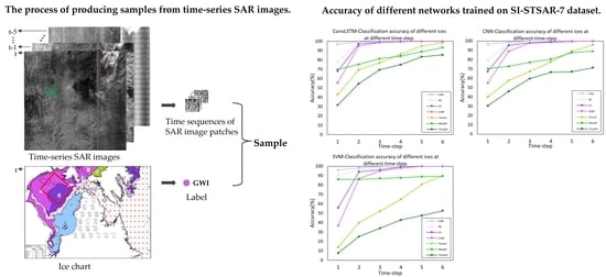
- A complete method for constructing a spatiotemporal dataset for sea ice classification is provided. In sample production, the ice concentration principle, ice development principle, and cross-subswath principle are creatively proposed to improve the quality of the dataset. Among them, the cross-subswath principle can effectively alleviate the impact of Sentinel-1 thermal noise on sea ice classification, especially in the first subswath region, which provides a reference scheme for the region subject to high thermal noise in sea ice research.
- Using the proposed method, we provide a large spatiotemporal dataset for sea ice classification based on Sentinel-1 SAR images. This is the first large labeled sea ice SAR dataset that provides both spatial and temporal information. We also preliminarily studied the impact of time-step (the number of consecutive SAR scenes) on sea ice classification.
- Comprehensive evaluation results of three advanced classification algorithms based on accuracy and kappa coefficient, are presented as the benchmarks of sea ice classification using SI-STSAR-7.
2. Dataset Construction
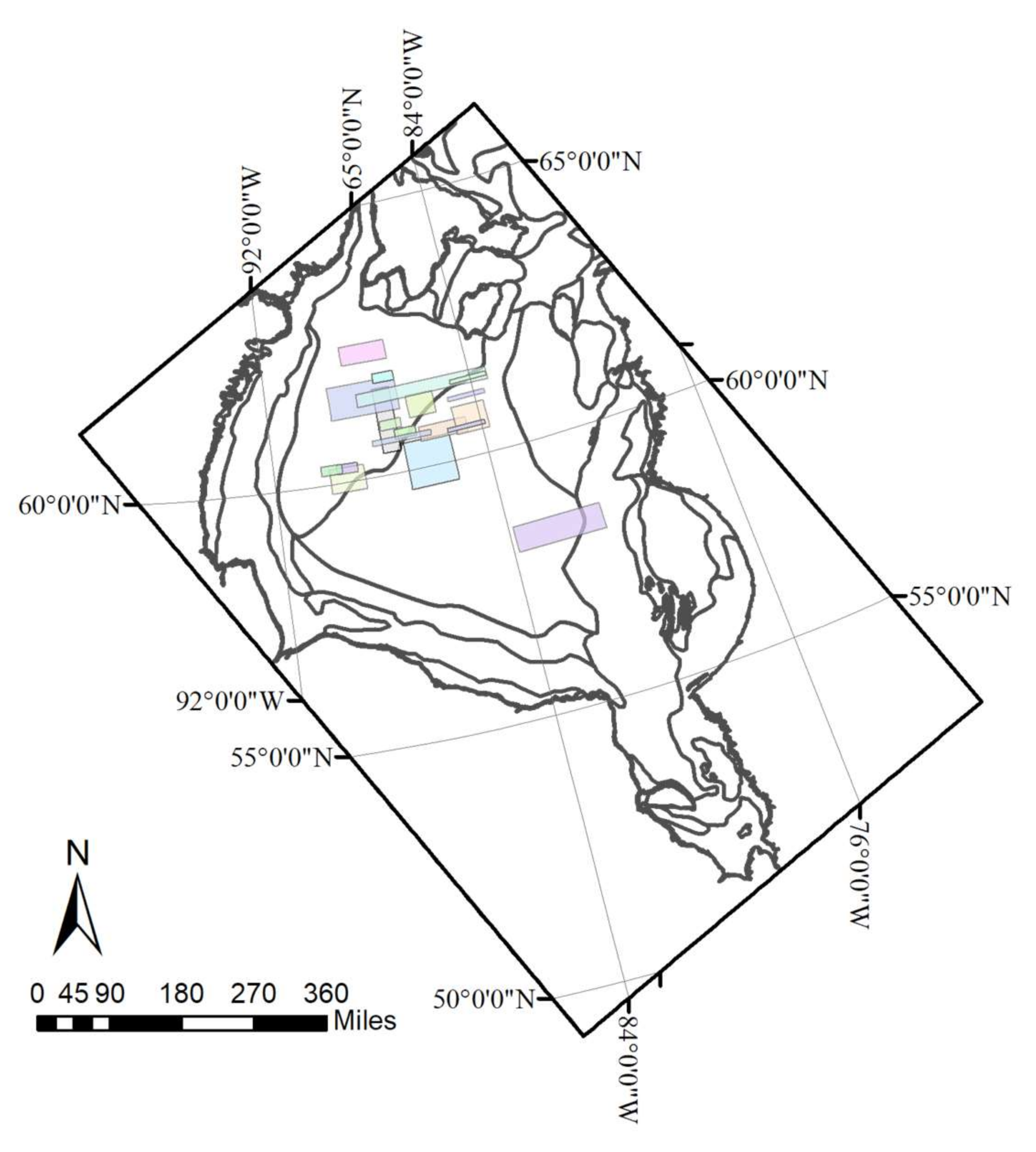
2.1. SAR Source and Study Area
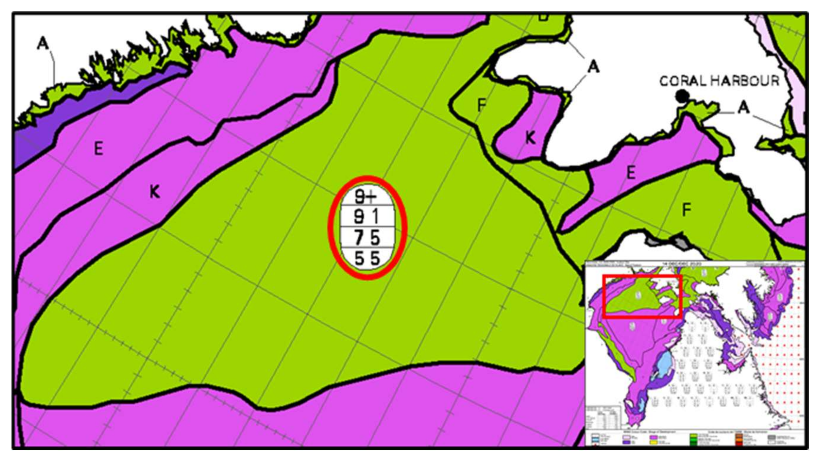
2.2. Reference Data
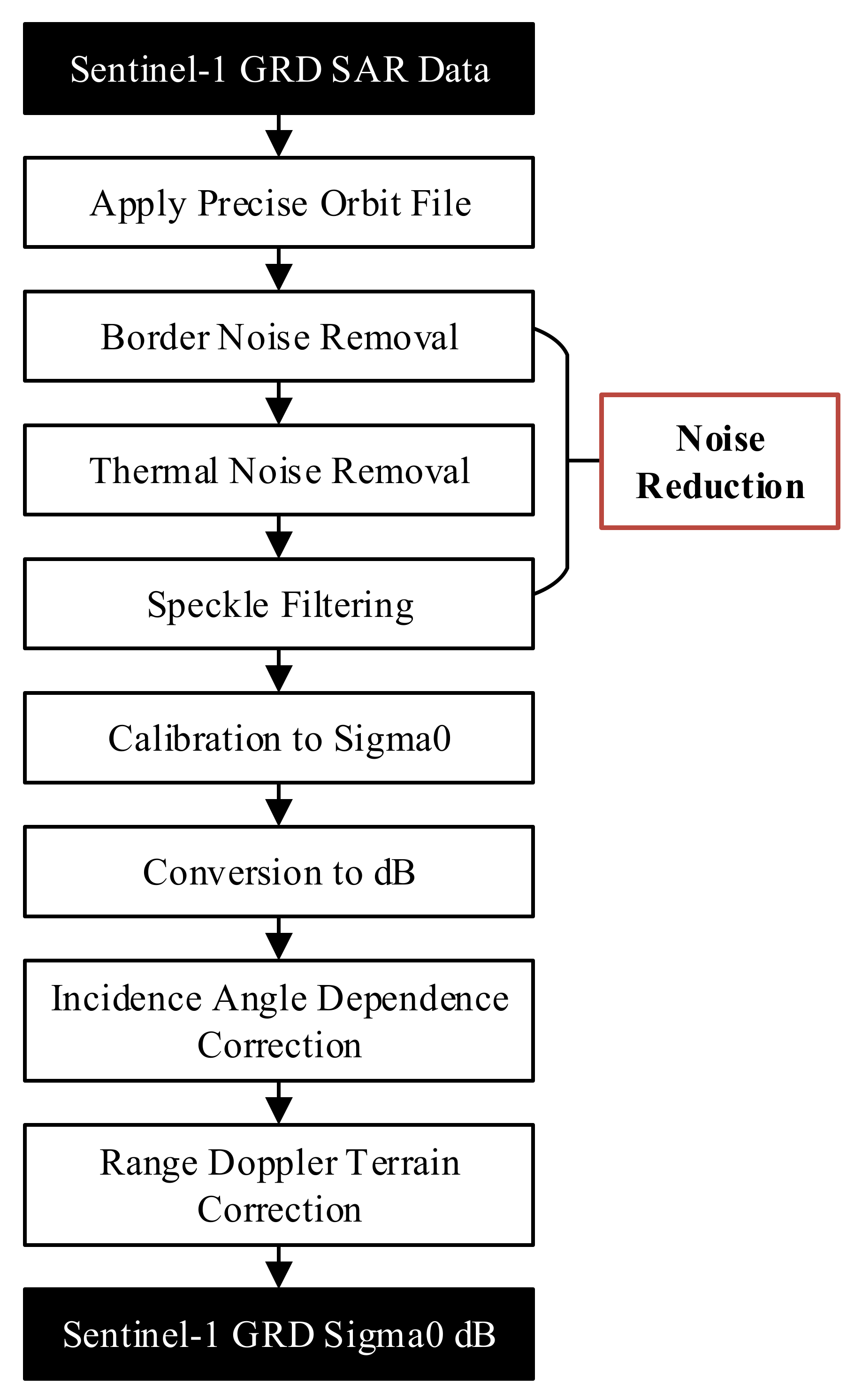
2.3. SAR Image Preprocessing
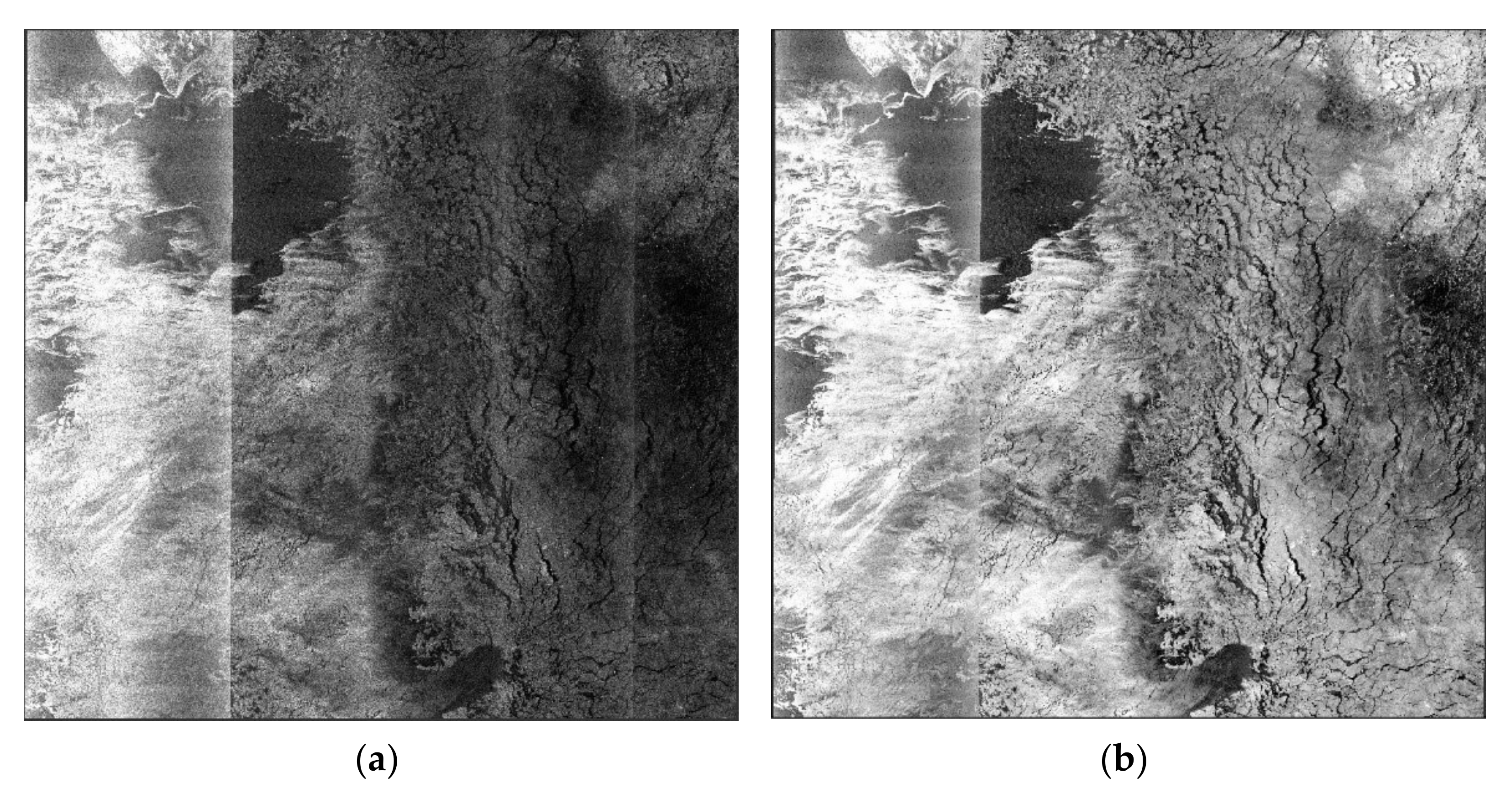
2.3.1. Noise Reduction
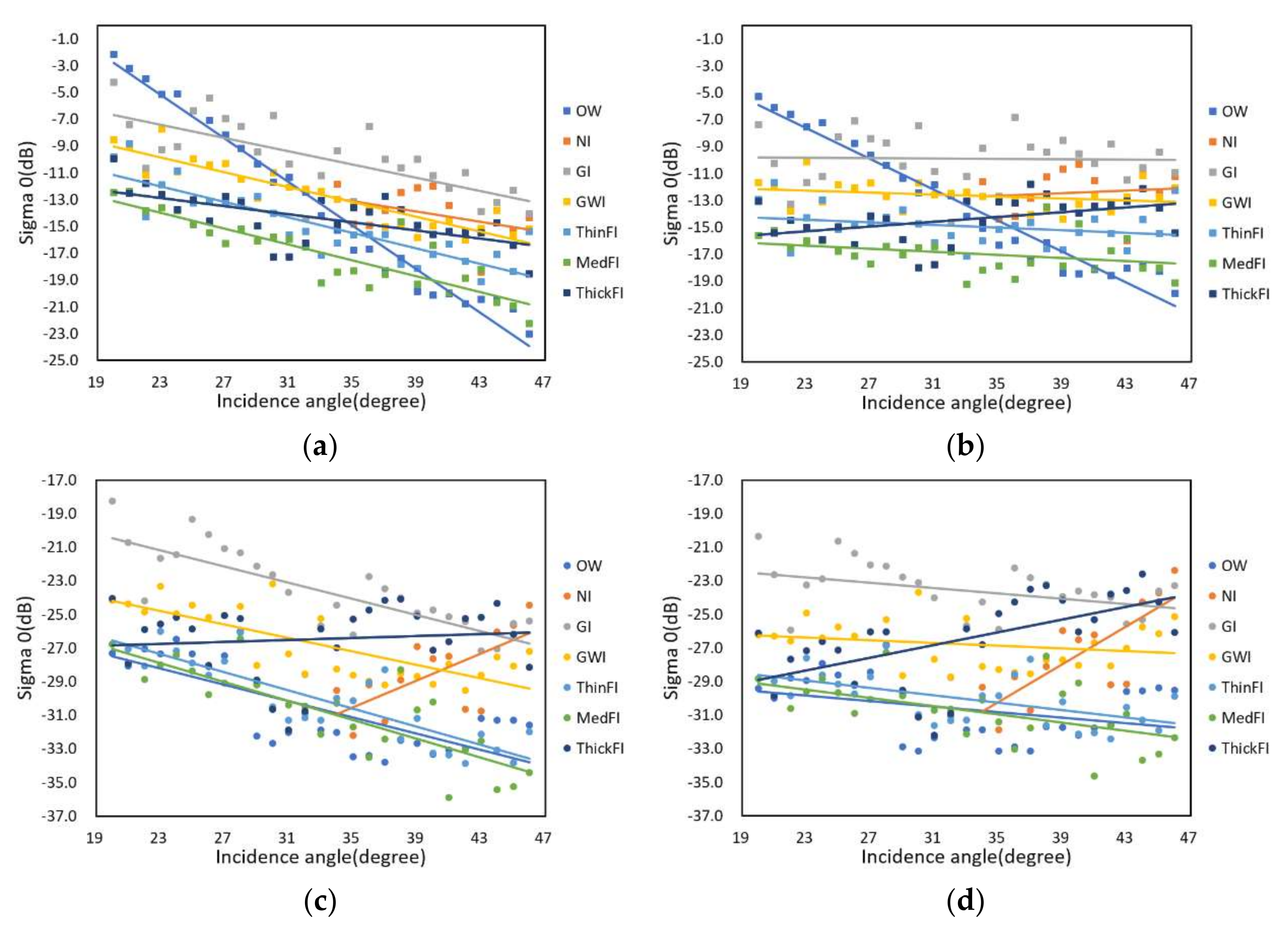
2.3.2. Incidence Angle Dependence Correction
2.4. Sample Production
- Concentration principle
- Ice development principle
- Cross-subswath principle
- Boundary principle
3. Experiments
3.1. Baseline Methods
3.2. Evaluation Metrics
- Accuracy: The proportion of correctly classified samples to total samples.
- Accuracy of each ice class: The proportion of correctly classified samples of a given class to total samples of that class.
- Kappa coefficient: An indicator for measuring the consistency of multi-class models, which is based on the confusion matrix. The formula is as follows.
3.3. Implementation
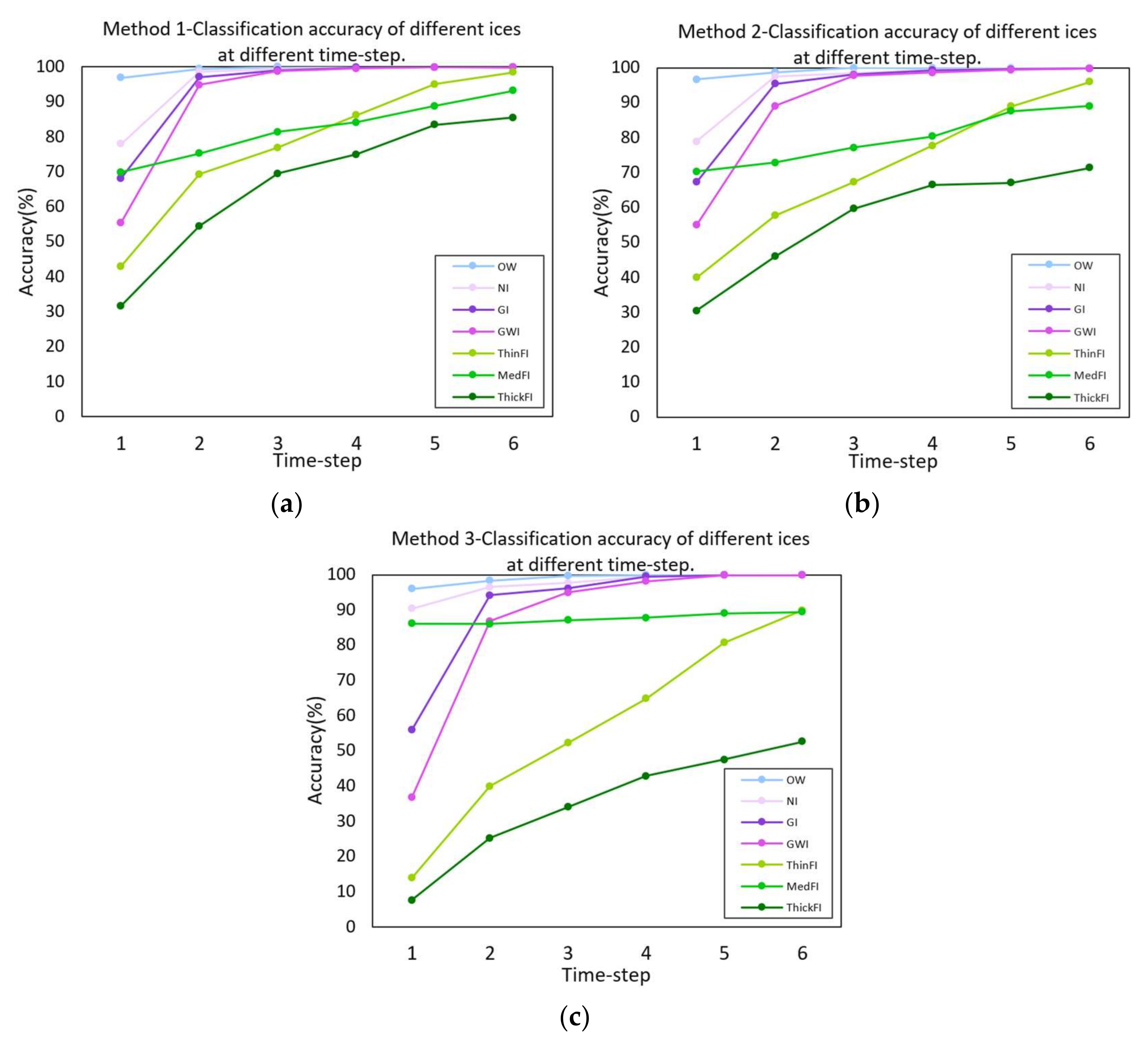
3.4. Sea Ice Classification Performance on SI-STSAR-7
3.5. Sample-Producing Principle Verification
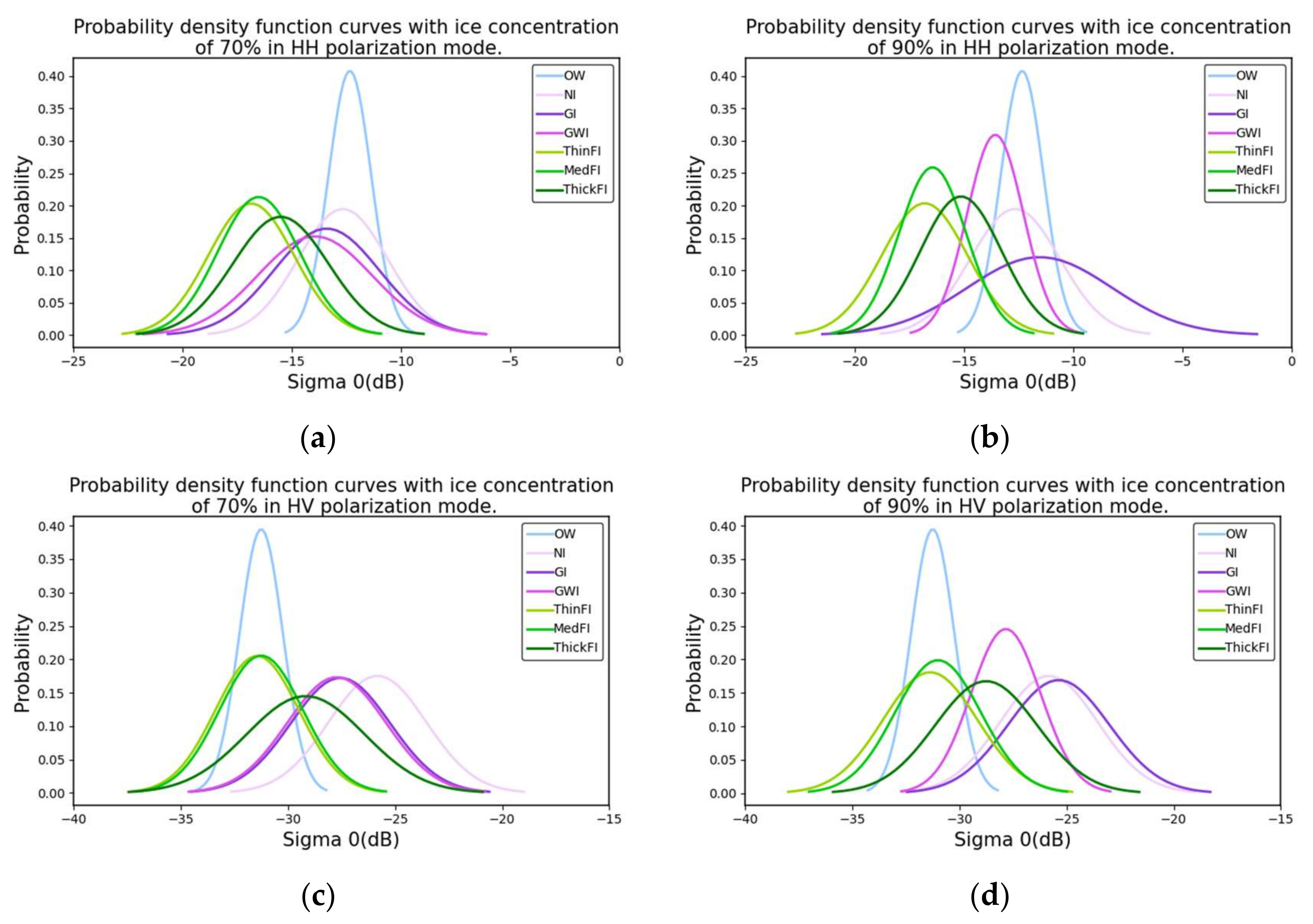
3.5.1. Concentration Principle
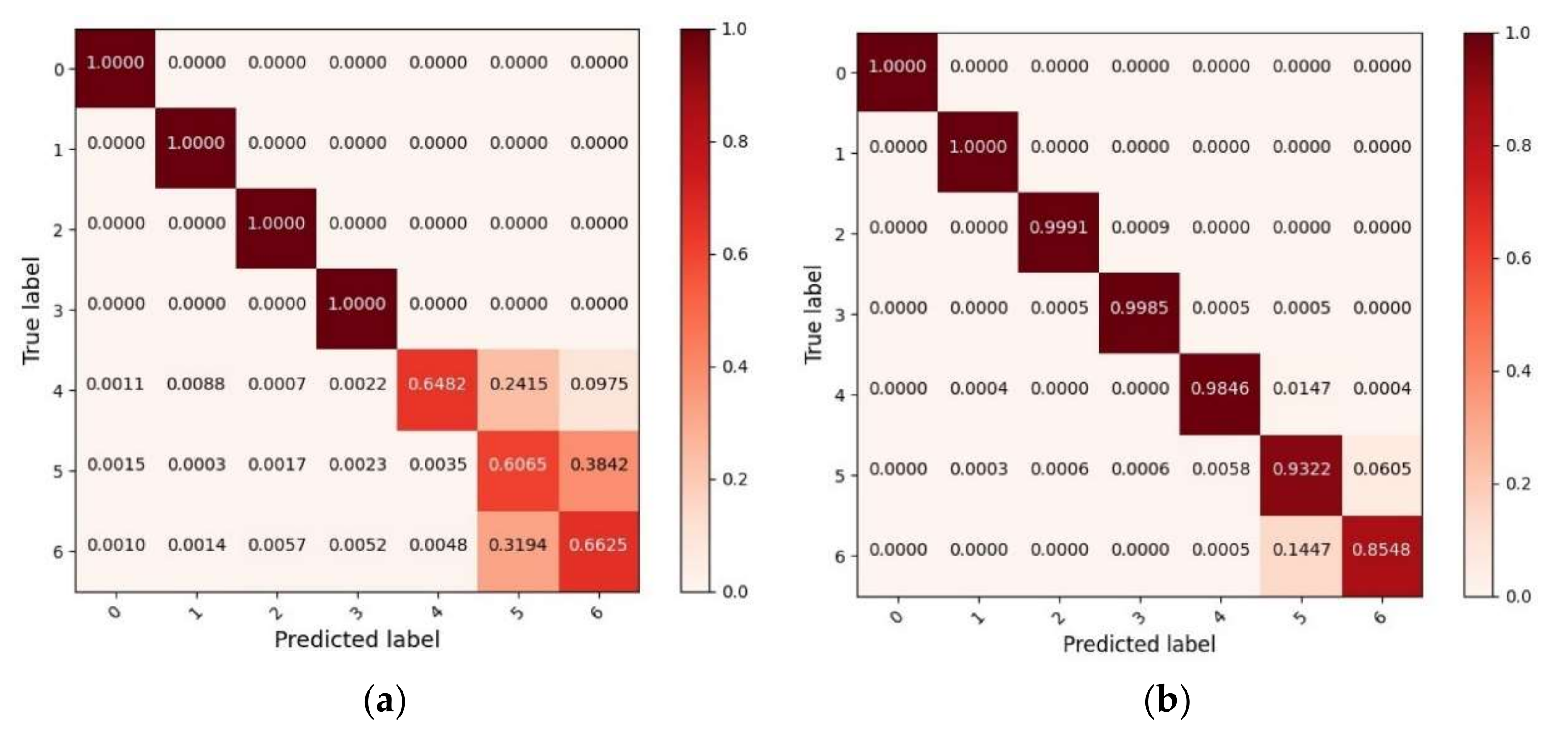
3.5.2. Ice Development Principle
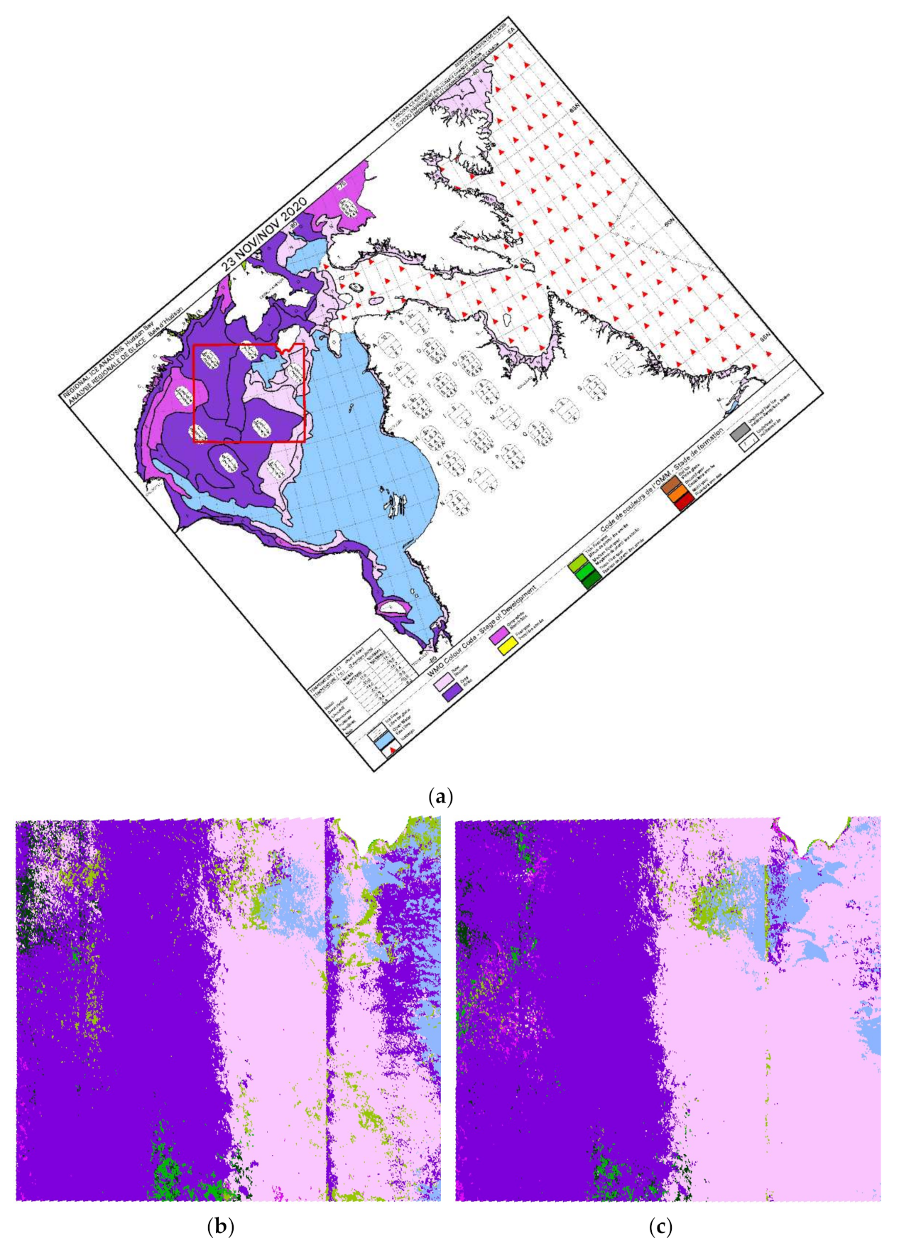
3.5.3. Cross-Subswath Principle
4. Conclusions
Author Contributions
Funding
Data Availability Statement
Acknowledgments
Conflicts of Interest
References
- Vihma, T. Effects of Arctic Sea Ice Decline on Weather and Climate: A Review. Surv. Geophys. 2014, 35, 1175–1214. [Google Scholar] [CrossRef] [Green Version]
- Wilson, K.J.; Falkingham, J.; Melling, H.; Abreu, R.D. Shipping in the Canadian Arctic: Other Possible Climate Change Scenarios. In Proceedings of the IGARSS 2004, 2004 IEEE International Geoscience and Remote Sensing Symposium, Anchorage, AK, USA, 20–24 September 2004; Volume 1853, pp. 1853–1856. [Google Scholar]
- Karvonen, J. Baltic Sea Ice Concentration Estimation Based on C-Band Dual-Polarized SAR Data. IEEE Trans. Geosci. Remote Sens. 2014, 52, 5558–5566. [Google Scholar] [CrossRef]
- Clausi, D.A. An Analysis of Co-occurrence Texture Statistics as a Function of Grey Level Quantization. Can. J. Remote Sens. 2002, 28, 45–62. [Google Scholar] [CrossRef]
- Deng, H.; Clausi, D.A. Unsupervised Segmentation of Synthetic Aperture Radar Sea Ice Imagery Using a Novel Markov Random Field Model. IEEE Trans. Geosci. Remote 2005, 43, 528–538. [Google Scholar] [CrossRef]
- Ochilov, S.; Clausi, D.A. Operational SAR Sea-Ice Image Classification. IEEE Trans. Geosci. Remote 2012, 50, 4397–4408. [Google Scholar] [CrossRef]
- Ressel, R.; Frost, A.; Lehner, S. A Neural Network-Based Classification for Sea Ice Types on X-Band SAR Images. IEEE J. Sel. Top. Appl. Earth Obs. Remote Sens. 2015, 8, 1–9. [Google Scholar] [CrossRef]
- Ressel, R.; Singha, S.; Lehner, S.; Rösel, A.; Spreen, G. Investigation into Different Polarimetric Features for Sea Ice Classification Using X-Band Synthetic Aperture Radar. IEEE J. Sel. Top. Appl. Earth Obs. Remote Sens. 2016, 9, 3131–3143. [Google Scholar] [CrossRef] [Green Version]
- Liu, H.; Guo, H.; Zhang, L. SVM-Based Sea Ice Classification Using Textural Features and Concentration From RADARSAT-2 Dual-Pol ScanSAR Data. IEEE J. Sel. Top. Appl. Earth Obs. Remote Sens. 2015, 8, 1601–1613. [Google Scholar] [CrossRef]
- Zhang, L.; Liu, H.; Gu, X.; Guo, H.; Chen, J.; Liu, G. Sea Ice Classification Using TerraSAR-X ScanSAR Data With Removal of Scalloping and Interscan Banding. IEEE J. Sel. Top. Appl. Earth Obs. Remote Sens. 2019, 12, 589–598. [Google Scholar] [CrossRef]
- Yang, K.-S.; Kiang, J.-F. Comparison of Algorithms and Input Vectors for Sea-Ice Classification with L-Band PolSAR Data. Prog. Electromagn. Res. B 2019, 84, 1–21. [Google Scholar] [CrossRef] [Green Version]
- Boulze, H.; Korosov, A.; Brajard, J. Classification of Sea Ice Types in Sentinel-1 SAR Data Using Convolutional Neural Networks. Remote Sens. 2020, 12, 2165. [Google Scholar] [CrossRef]
- Cheng, G.; Zhou, P.; Han, J. Learning Rotation-Invariant Convolutional Neural Networks for Object Detection in VHR Optical Remote Sensing Images. IEEE Trans. Geosci. Remote 2016, 54, 7405–7415. [Google Scholar] [CrossRef]
- Xia, G.-S.; Bai, X.; Ding, J.; Zhu, Z.; Belongie, S.; Luo, J.; Datcu, M.; Pelillo, M.; Zhang, L. DOTA: A Large-Scale Dataset for Object Detection in Aerial Images. In Proceedings of the 2018 IEEE/CVF Conference on Computer Vision and Pattern Recognition, Salt Lake City, UT, USA, 18–23 June 2018; pp. 3974–3983. [Google Scholar]
- Di, Y.; Jiang, Z.; Zhang, H. A Public Dataset for Fine-Grained Ship Classification in Optical Remote Sensing Images. Remote Sens. 2021, 13, 747. [Google Scholar] [CrossRef]
- Wang, Z.; Bai, L.; Song, G.; Zhang, J.; Tao, J.; Mulvenna, M.; Bond, R.R.; Chen, L. An Oil Well Dataset Derived from Satellite-Based Remote Sensing. Remote Sens. 2021, 13, 1132. [Google Scholar] [CrossRef]
- National Center for Atmospheric Research Staff (Ed.) The Climate Data Guide: Sea Ice Concentration Data: Overview, Comparison Table and Graphs; Last modified 11 September 2017. Available online: https://climatedataguide.ucar.edu/climate-data/sea-ice-concentration-data-overview-comparison-table-and-graphs (accessed on 30 August 2021).
- Khaleghian, S.; Ullah, H.; Kræmer, T.; Hughes, N.; Eltoft, T.; Marinoni, A. Sea Ice Classification of SAR Imagery Based on Convolution Neural Networks. Remote Sens. 2021, 13, 1734. [Google Scholar] [CrossRef]
- Jackson, C. Synthetic Aperture Radar Marine User’s Manual; National Environmental Satellite, Data, and Information Service (NESDIS): Washington, DC, USA, 2004. [Google Scholar]
- Dierking, W. Sea Ice Monitoring by Synthetic Aperture Radar. Oceanography 2013, 26, 100–111. [Google Scholar] [CrossRef]
- Scheuchl, B.; Flett, D.; Caves, R.; Cumming, I. Potential of RADARSAT-2 for Operational Sea Ice Monitoring. Can. J. Remote Sens. 2004, 30, 448–461. [Google Scholar] [CrossRef]
- Horstmann, J.; Falchetti, S.; Wackerman, C.; Maresca, S.; Caruso, M.J.; Graber, H.C. Tropical Cyclone Winds Retrieved From C-Band Cross-Polarized Synthetic Aperture Radar. IEEE Trans. Geosci. Remote 2015, 53, 2887–2898. [Google Scholar] [CrossRef] [Green Version]
- Moen, M.-A.N.; Anfinsen, S.N.; Doulgeris, A.P.; Renner, A.H.H.; Gerland, S. Assessing Polarimetric SAR Sea-ice Classifications Using Consecutive Day Images. Ann. Glaciol. 2015, 56, 285–294. [Google Scholar] [CrossRef] [Green Version]
- Zakhvatkina, N.; Smirnov, V.; Bychkova, I. Satellite SAR Data-based Sea Ice Classification: An Overview. Geosciences 2019, 9, 152. [Google Scholar] [CrossRef] [Green Version]
- Aldenhoff, W.; Heuzé, C.; Eriksson, L.E.B. Comparison of Ice/Water Classification in Fram Strait from C- and L-band SAR imagery. Ann. Glaciol. 2018, 59, 112–123. [Google Scholar] [CrossRef] [Green Version]
- Chen, S.; Shokr, M.; Li, X.; Ye, Y.; Zhang, Z.; Hui, F.; Cheng, X. MYI Floes Identification Based on the Texture and Shape Feature from Dual-Polarized Sentinel-1 Imagery. Remote Sens. 2020, 12, 3221. [Google Scholar] [CrossRef]
- Malmgren-Hansen, D.; Pedersen, L.T.; Nielsen, A.A.; Kreiner, M.B.; Saldo, R.; Skriver, H.; Lavelle, J.; Buus-Hinkler, J.; Krane, K.H. A Convolutional Neural Network Architecture for Sentinel-1 and AMSR2 Data Fusion. IEEE Trans. Geosci. Remote 2021, 59, 1890–1902. [Google Scholar] [CrossRef]
- Joint WMO-IOC Technical Commission for Oceanography and Marine Meteorology. Ice Chart Colour Code Standard; Version 1.0; World Meteorological Organization & Intergovernmental Oceanographic Commission: Geneva, Switzerland, 2014. [Google Scholar]
- Petrou, Z.I.; Tian, Y. Prediction of Sea Ice Motion with Recurrent Neural Networks. In Proceedings of the 2017 IEEE International Geoscience and Remote Sensing Symposium (IGARSS), Fort Worth, TX, USA, 23–28 July 2017; pp. 5422–5425. [Google Scholar]
- Chi, J.; Kim, H.-C. Prediction of Arctic Sea Ice Concentration Using a Fully Data Driven Deep Neural Network. Remote Sens. 2017, 9, 1305. [Google Scholar] [CrossRef] [Green Version]
- Song, W.; Li, M.; Gao, W.; Huang, D.; Ma, Z.; Liotta, A.; Perra, C. Automatic Sea-Ice Classification of SAR Images Based on Spatial and Temporal Features Learning. IEEE Trans. Geosci. Remote 2021, 59, 9887–9901. [Google Scholar] [CrossRef]
- Manual of Ice (MANICE); Government of Canada: Ottawa, ON, Canada. Available online: https://www.canada.ca/en/environment-climate-change/services/weather-manuals-documentation/manice-manual-of-ice.html (accessed on 12 June 2021).
- Lee, J.S.; Jurkevich, L.; Dewaele, P.; Wambacq, P.; Oosterlinck, A. Speckle Filtering of Synthetic Aperture Radar Images: A Review. Remote Sens. Rev. 1994, 8, 313–340. [Google Scholar] [CrossRef]
- Park, J.-W.; Korosov, A.A.; Babiker, M.; Sandven, S.; Won, J.-S. Efficient Thermal Noise Removal for Sentinel-1 TOPSAR Cross-Polarization Channel. IEEE Trans. Geosci. Remote 2018, 56, 1555–1565. [Google Scholar] [CrossRef]
- Hajduch, G.; Miranda, N.; Piantanida, R.; Meadows, P.; Vincent, P.; Franceschi, N. Thermal Denoising of Products Generated by the S-1 IPF; Report number: DI-MPC-TN, MPC-0392; Project: Sentinel-1 Mission Performance Centre. 28 November 2017. Available online: https://sentinel.esa.int/documents/247904/2142675/Thermal-Denoising-of-Products-Generated-by-Sentinel-1-IPF (accessed on 20 May 2021).
- S-1 Mission Performance Center. Sentinel-1 Product Definition; S1-RS-MDA-52-7440, Issue/Revision 2/7; MacDonald Dettwiler: Richmond, BC, USA, 25 March 2016. [Google Scholar]
- The Sentinel-1 Toolbox. Available online: http://step.esa.int/main/download/snap-download/ (accessed on 16 June 2021).
- Filipponi, F. Sentinel-1 GRD Preprocessing Workflow. Proceedings 2019, 18, 6201. [Google Scholar] [CrossRef] [Green Version]
- SNAP Sentinel-1 Toolbox Course. Available online: https://sa.catapult.org.uk/events/snap-sentinel-1-toolbox-course/ (accessed on 13 June 2021).
- Mäkynen, M.; Karvonen, J. Incidence Angle Dependence of First-Year Sea Ice Backscattering Coefficient in Sentinel-1 SAR Imagery Over the Kara Sea. IEEE Trans. Geosci. Remote 2017, 55, 6170–6181. [Google Scholar] [CrossRef]
- Komarov, A.S.; Buehner, M. Detection of First-Year and Multi-Year Sea Ice from Dual-Polarization SAR Images Under Cold Conditions. IEEE Trans. Geosci. Remote 2019, 57, 9109–9123. [Google Scholar] [CrossRef]
- Aldenhoff, W.; Eriksson, L.E.B.; Ye, Y.; Heuzé, C. First-Year and Multiyear Sea Ice Incidence Angle Normalization of Dual-Polarized Sentinel-1 SAR Images in the Beaufort Sea. IEEE J. Sel. Top. Appl. Earth Obs. Remote Sens. 2020, 13, 1540–1550. [Google Scholar] [CrossRef]
- Nghiem, S.V.; Bertoia, C. Study of Multi-Polarization C-Band Backscatter Signatures for Arctic Sea Ice Mapping with Future Satellite SAR. Can. J. Remote Sens. 2001, 27, 387–402. [Google Scholar] [CrossRef]
- Park, J.-W.; Korosov, A.; Babiker, M.; Kim, H.-C. Automated Sea Ice Classification Using Sentinel-1 Imagery. In Proceedings of the IGARSS 2019-2019 IEEE International Geoscience and Remote Sensing Symposium, Yokohama, Japan, 28 July–2 August 2019; pp. 4008–4011. [Google Scholar]
- Shi, X.; Chen, Z.; Wang, H.; Yeung, D.-Y.; Wong, W.-K.; Woo, W.-C. Convolutional LSTM Network: A Machine Learning Approach for Precipitation Nowcasting. Comput. Sci. 2015, 1, 802–810. [Google Scholar]
- Ioffe, S.; Szegedy, C. Batch Normalization: Accelerating Deep Network Training by Reducing Internal Covariate Shift. In Proceedings of the 32nd International Conference on International Conference on Machine Learning, Lille, France, 6–11 July 2015; pp. 448–456. [Google Scholar]
- Zakhvatkina, N.; Korosov, A.; Muckenhuber, S.; Sandven, S.; Babiker, M. Operational Algorithm for Ice/Water Classification on Dual-polarized RADARSAT-2 Images. Cryosphere 2017, 11, 33–46. [Google Scholar] [CrossRef] [Green Version]
- Hong, D.-B.; Yang, C.-S. Automatic Discrimination Approach of Sea Ice in the Arctic Ocean Using Sentinel-1 Extra Wide Swath Dual-polarized SAR Data. Int. J. Remote Sens. 2018, 39, 4469–4483. [Google Scholar] [CrossRef]
- Leigh, S.; Wang, Z.; Clausi, D.A. Automated Ice–Water Classification Using Dual Polarization SAR Satellite Imagery. IEEE Trans. Geosci. Remote 2014, 52, 5529–5539. [Google Scholar] [CrossRef]
- Tan, W.; Li, J.; Xu, L.; Chapman, M.A. Semiautomated Segmentation of Sentinel-1 SAR Imagery for Mapping Sea Ice in Labrador Coast. IEEE J. Sel. Top. Appl. Earth Obs. Remote Sens. 2018, 11, 1419–1432. [Google Scholar] [CrossRef]


| No. | Satellite | Size (Pixels) | Incidence Angle (Degree) | Coordinate |
|---|---|---|---|---|
| 1 | Sentinel-1A | 10,563 × 9998 | 19.23–46.90 | 58.73°N–63.06°N, 81.90°W–91.10°W |
| 2 | Sentinel-1B | 10,642 × 9991 | 19.09–46.94 | 59.09°N–63.43°N, 81.64°W–91.02°W |
| Stage of Development | Thickness (cm) | Code | Color |
|---|---|---|---|
| Open Water (<1/10 Ice) |  | ||
| New Ice | 10 | 1 |  |
| Grey Ice | 10–15 | 4 |  |
| Grey-White Ice | 15–30 | 5 |  |
| Thin First-Year Ice | 30–70 | 7 |  |
| Medium First-Year Ice | 70–120 | 1. |  |
| Thick First-Year Ice | 120 | 4. |  |
| Sample | SAR Date | ||||||||
|---|---|---|---|---|---|---|---|---|---|
| … | 20210117 | 20210123 | 20210129 | 20210204 | 20210210 | 20210216 | 20210222 | … | |
| sample 1 | … | ThinFI, 0.7; MedFI, 0.3 | ThinFI, 0.5; MedFI, 0.5 | ThinFI, 0.3; MedFI, 0.7 | MedFI, 0.9 | … | … | … | … |
| sample 2 | … | … | ThinFI, 0.5; MedFI, 0.5 | ThinFI, 0.3; MedFI, 0.7 | MedFI, 0.9 | MedFI, 0.9+ | … | … | … |
| sample 3 | … | … | … | ThinFI, 0.3; MedFI, 0.7 | MedFI, 0.9 | MedFI, 0.9+ | MedFI, 0.9+ | … | … |
| sample 4 | … | … | … | … | MedFI, 0.9 | MedFI, 0.9+ | MedFI, 0.9+ | MedFI, 0.9+ | … |
| SAR Date | Total Concentration | Main Ice Type, Concentration | SAR Date | Total Concentration | Main Ice Type, Concentration |
|---|---|---|---|---|---|
| OW | MedFI | ||||
| 20191130 | —— | —— | 20200216 | 0.9+ | MedFI, 0.9+ |
| 20201118 | —— | —— | 20200222 | 0.9+ | MedFI, 0.9+ |
| NI | 20200228 | 0.9+ | MedFI, 0.9+ | ||
| 20191209 | 0.9 | NI, 0.5 | 20200305 | 0.9+ | MedFI, 0.9+ |
| 20201124 | 0.9+ | NI, 0.7 | 20200311 | 0.9+ | MedFI, 0.9− |
| GI | 20200317 | 0.9+ | MedFI, 0.9+ | ||
| 20191206 | 0.9− | GI, 0.8 | 20210204 | 0.9+ | MedFI, 0.9 |
| 20201124 | 0.9− | GI, 0.8 | 20210210 | 0.9+ | MedFI, 0.9+ |
| GWI | 20210216 | 0.9+ | MedFI, 0.9+ | ||
| 20191206 | 0.9 | GWI, 0.8 | 20210222 | 0.9+ | MedFI, 0.9+ |
| 20201130 | 0.9+ | GWI, 0.9+ | 20210228 | 0.9+ | MedFI, 0.9− |
| 20201206 | 0.9+ | GWI, 0.8 | 20210306 | 0.9+ | MedFI, 0.9+ |
| ThinFI | 20210312 | 0.9+ | MedFI, 0.9− | ||
| 20191230 | 0.9+ | ThinFI, 0.9+ | ThickFI | ||
| 20200105 | 0.9+ | ThinFI, 0.9+ | 20200410 | 0.9+ | ThickFI, 0.9 |
| 20200111 | 0.9+ | ThinFI, 0.9− | 20200416 | 0.9+ | ThickFI, 0.9 |
| 20200117 | 0.9+ | ThinFI, 0.9− | 20200422 | 0.9+ | ThickFI, 0.9+ |
| 20200123 | 0.9+ | ThinFI, 0.9+ | 20200428 | 0.9+ | ThickFI, 0.9+ |
| 20201212 | 0.9+ | ThinFI, 0.9 | 20200504 | 0.9+ | ThickFI, 0.9+ |
| 20201218 | 0.9+ | ThinFI, 0.9+ | 20200510 | 0.9− | ThickFI, 0.9− |
| 20201224 | 0.9+ | ThinFI, 0.9+ | 20200516 | 0.9− | ThickFI, 0.9− |
| 20201230 | 0.9+ | ThinFI, 0.9+ | 20200522 | 0.9+ | ThickFI, 0.9+ |
| 20210105 | 0.9+ | ThinFI, 0.9 | 20210423 | 0.9+ | ThickFI, 0.9 |
| 20210111 | 0.9+ | ThinFI, 0.9 | 20210429 | 0.9+ | ThickFI, 0.9+ |
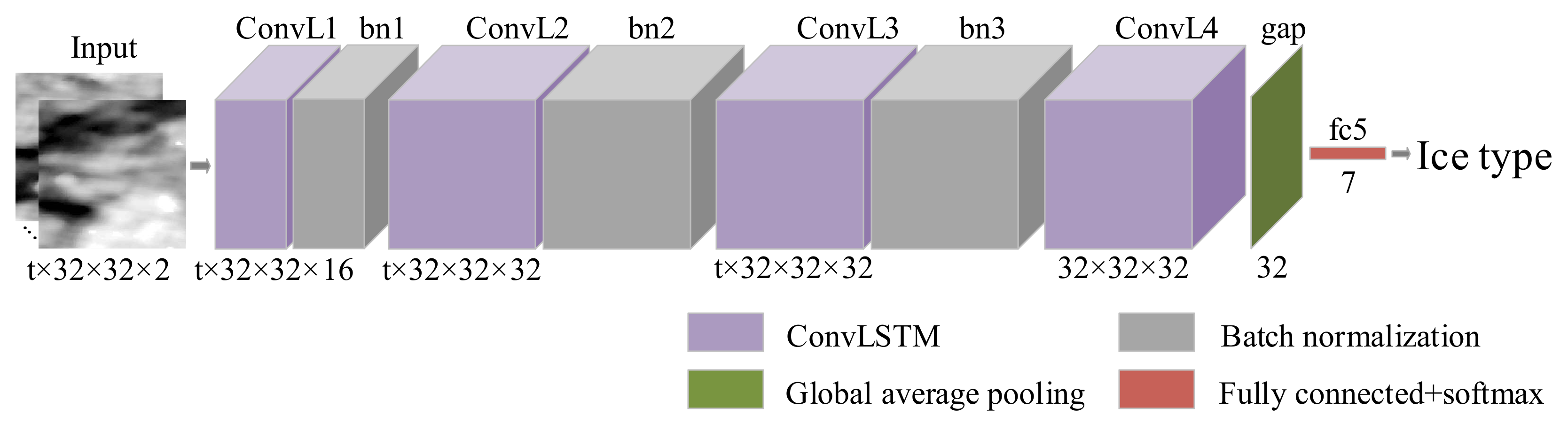
| Layer | Parameter | Activation Function |
|---|---|---|
| Input | 2 | —— |
| ConvLSTM 1 (ConvL1) | 3), padding same, return_sequences true | Sigmoid |
| Batch Normalization 1 (bn1) | —— | —— |
| ConvLSTM 2 (ConvL2) | 323), padding same, return_sequences true | Sigmoid |
| Batch Normalization 2 (bn2) | —— | —— |
| ConvLSTM 3 (ConvL3) | 3), padding same, return_sequences true | Sigmoid |
| Batch Normalization 3 (bn3) | —— | —— |
| ConvLSTM 4 (ConvL4) | 3), padding same, return_sequences false | Sigmoid |
| Global Average Pooling (gap) | —— | —— |
| Fully Connected (fc5) | 7 nodes | Softmax |
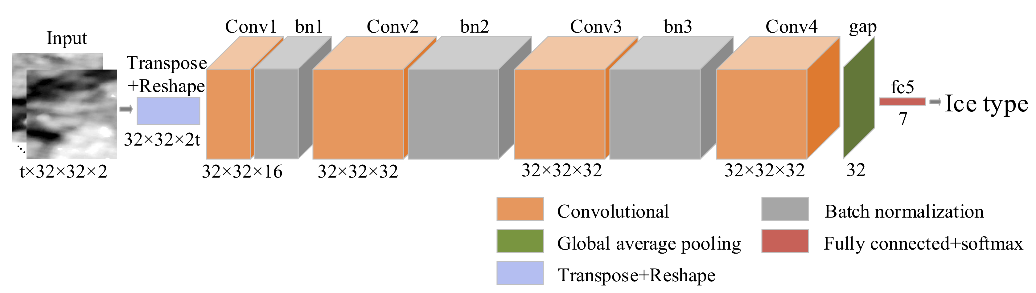
| Layer | Parameter | Activation Function |
|---|---|---|
| Input | 2 | —— |
| Transpose | —— | —— |
| Reshape | —— | —— |
| Convolutional 1 (Conv1) | 3), padding same | Sigmoid |
| Batch Normalization 1 (bn1) | —— | —— |
| Convolutional 2 (Conv2) | 323), padding same | Sigmoid |
| Batch Normalization 2 (bn2) | —— | —— |
| Convolutional 3 (Conv3) | 3), padding same | Sigmoid |
| Batch Normalization 3 (bn3) | —— | —— |
| Convolutional 4 (Conv4) | 3), padding same | Sigmoid |
| Global Average Pooling (gap) | —— | —— |
| Fully Connected (fc5) | 7 nodes | Softmax |
| Baseline Method | Method 1 | Method 2 | Method 3 | |||
|---|---|---|---|---|---|---|
| Time-step | Accuracy (%) | Kappa | Accuracy (%) | Kappa | Accuracy (%) | Kappa |
| 1 | 62.84 | 0.56 | 62.15 | 0.55 | 54.58 | 0.45 |
| 2 | 82.65 | 0.79 | 78.02 | 0.74 | 74.56 | 0.69 |
| 3 | 88.02 | 0.85 | 83.89 | 0.81 | 79.53 | 0.75 |
| 4 | 91.08 | 0.89 | 87.57 | 0.85 | 83.95 | 0.81 |
| 5 | 94.68 | 0.93 | 91.18 | 0.89 | 87.76 | 0.85 |
| 6 | 96.44 | 0.95 | 93.31 | 0.92 | 90.03 | 0.88 |
| Sea Ice Class | Dataset 1 | Dataset 2 |
|---|---|---|
| OW | Meet the ice development principle. | Meet the ice development principle. |
| NI | Meet the ice development principle. | Meet the ice development principle. |
| GI | Meet the ice development principle. | Meet the ice development principle. |
| GWI | Meet the ice development principle. | Meet the ice development principle. |
| ThinFI | The ice concentration has just reached 90%. | Meet the ice development principle. |
| MedFI | The ice concentration has just reached 90%. | Meet the ice development principle. |
| ThickFI | The ice concentration has just reached 90%. | Meet the ice development principle. |
Publisher’s Note: MDPI stays neutral with regard to jurisdictional claims in published maps and institutional affiliations. |
© 2021 by the authors. Licensee MDPI, Basel, Switzerland. This article is an open access article distributed under the terms and conditions of the Creative Commons Attribution (CC BY) license (https://creativecommons.org/licenses/by/4.0/).
Share and Cite
Song, W.; Gao, W.; He, Q.; Liotta, A.; Guo, W. SI-STSAR-7: A Large SAR Images Dataset with Spatial and Temporal Information for Classification of Winter Sea Ice in Hudson Bay. Remote Sens. 2022, 14, 168. https://0-doi-org.brum.beds.ac.uk/10.3390/rs14010168
Song W, Gao W, He Q, Liotta A, Guo W. SI-STSAR-7: A Large SAR Images Dataset with Spatial and Temporal Information for Classification of Winter Sea Ice in Hudson Bay. Remote Sensing. 2022; 14(1):168. https://0-doi-org.brum.beds.ac.uk/10.3390/rs14010168
Chicago/Turabian StyleSong, Wei, Wen Gao, Qi He, Antonio Liotta, and Weiqi Guo. 2022. "SI-STSAR-7: A Large SAR Images Dataset with Spatial and Temporal Information for Classification of Winter Sea Ice in Hudson Bay" Remote Sensing 14, no. 1: 168. https://0-doi-org.brum.beds.ac.uk/10.3390/rs14010168