Article

Attributing the Evapotranspiration Trend in the Upper and Middle Reaches of Yellow River Basin Using Global Evapotranspiration Products

1
Key Laboratory of Soil and Water Conservation on the Loess Plateau of Ministry of Water Resources, Yellow River Institute of Hydraulic Research, Yellow River Conservancy Commission, Zhengzhou 450003, China
2
Henan Key Laboratory of Ecological Environment Protection and Restoration of the Yellow River Basin, Zhengzhou 450003, China
3
School of Water Conservancy Engineering, Zhengzhou University, Zhengzhou 450001, China
4
Institute of Geographic Sciences and Natural Resources Research, Chinese Academy of Sciences, Beijing 100101, China
*
Author to whom correspondence should be addressed.
Submission received: 20 November 2021 / Revised: 27 December 2021 / Accepted: 29 December 2021 / Published: 31 December 2021
(This article belongs to the Special Issue Remote Sensing for Climate Extremes and Water Resources)

Abstract

:
Climate variation and underlying surface dynamics have caused a significant change in the trend of evapotranspiration (ET) in the Yellow River Basin (YRB) over the last two decades. Combined with the measured rainfall, runoff and gravity recovery and climate experiment (GRACE) product, five global ET products were firstly merged using a linear weighting method. Linear slope, “two-step” multiple regression, partial differential, and residual methods were then employed to explore the quantitative impacts of precipitation (PCPN), temperature (Temp), sunshine duration (SD), vapor pressure deficit (VPD), wind speed (WS), leaf area index (LAI), and the residual factors (e.g., microtopography changes, irrigation, etc.) on the ET trend in the YRB. The results show that: (1) The ET estimates were improved by merging five global ET products using the linear weighting method. The sensitivities of climatic factors and LAI on the ET trend can be separately calculated using proposed “two-step” statistical regression method; (2) the overall ET trend in the entire study area during 2000–2018 was 3.82 mm/yr, and the highest ET trend was observed in the Toudaoguai-Longmen subregion. ET trend was dominantly driven by vegetation greening, with an impact of 2.47 mm/yr and a relative impact rate of 51.16%. The results indicated that the relative impact rate of the residual factors (e.g., microtopography, irrigation, etc.) on the ET trend is up to 28.17%. The PCPN and VPD had increasing roles on the ET trend, with impacts of 0.45 mm/yr and 0.05 mm/yr, respectively, whereas the Temp, SD, and WS had decreasing impacts of –0.19 mm/yr, –0.15 mm/yr, and –0.17 mm/yr, respectively. (3) The spatial pattern of impact of specific influencing factor on the ET trend was determined by the spatial pattern of change trend slope of this factor and sensitivity of ET to this factor. ET trends of the source area and the Qingtongxia–Toudaoguai were dominated by the climatic factors, while the residual factors dominated the ET trend in the Tangnaihai–Qingtongxia area. The vegetation restoration was the dominant factor causing the increase in the ET in the middle reaches of the YRB, and the impact rates of the LAI were ranked as follows: Yanhe Rive > Wudinghe River > Fenhe River > Jinghe River > Beiluohe River > Qinhe River > Kuyehe River > Yiluohe River.

1. Introduction

Evapotranspiration (ET) is a key process in the terrestrial water cycle and the surface energy balance [1]. Evapotranspiration is a complex physical process, and the accurate estimation of the actual regional evapotranspiration has always remained difficult in water cycle studies [2]. Due to the influences of global climate change and drastic human activities, accurate simulation of the actual regional evapotranspiration and quantitative attribution of the ET dynamics are of great significance to clarifying regional water cycle processes, efficiently utilizing and optimizing the allocation of water resources, and evaluating the water resources required for ecological construction and sustainable socio-economic development [3,4,5].
The actual ET can be directly measured using measuring instruments, such as evapotranspiration meters, vorticity correlators, and large-aperture scintillators, at different scales from the meter level to the kilometer level [6]. However, the spatio-temporal dynamics of the ET at the regional scale cannot be easily obtained due to the limited number of field observations. As remote sensing techniques, climate models, and land surface models have been gradually integrated into the numerical simulation of the ET, scientists have developed numerous global and regional ET products. These products can be divided into three main categories based on the different estimation methods: (1) products interpolated using field measurements and machine learning methods (e.g., the marginal treatment effects method [7]); (2) products simulated using a remotely sensed evapotranspiration model (e.g., the moderate resolution imaging spectroradiometer [8] and probable maximum loss (PML) [9]); and (3) reanalysis data and products assimilated using different land surface models (e.g., the Japanese 55-year reanalysis [10], global land data assimilation system (GLDAS) [11], and global land evaporation Amsterdam model (GLEAM) [12]). However, there are large inconsistencies in the spatial and temporal distributions of the ET products due to the complex model structures, inaccurate physical parameters, and input datasets with different scales.
The Yellow River Basin (YRB) is an important ecological barrier in China, which feeds 12% of the country’s population with only 2% of the water resources provided by the national river runoff [13]. The average water resources per capita in the YRB is only 27% of the national average level [14]. Since 1999, ecological restoration projects (e.g., the returning farmland to forests and grassland project), have been implemented on the Loess Plateau. Currently, dramatic increases in the evapotranspiration induced by increasing vegetation biomass have led to a significant reduction in the natural runoff in the YRB [15,16,17], and dryness of the deeper soils in some areas of the Loess Plateau [18]. Moreover, the exploitation rate of the water resources in the YRB has been as high as 80%, far exceeding the 40% ecological alert line of the general level [19]. Therefore, attribution analysis of the effects of the climate change and the underlying surface changes on the ET trend in the upper and middle reaches of the YRB has significant implications for the ecological conservation and high-quality development of the YRB.
Recently, numerous studies on the spatio-temporal changes in the ET and its driving factors for the YRB have been conducted, and the results have revealed that climate change and underlying surface change have significantly affected the ET trend in the YRB. It is well known that precipitation is the main source of ET and predominantly control dynamics of hydrological cycle in water-limited regions [20]. Temperature [21], sunshine duration [22] associated with solar radiation, vapor pressure deficit [23], and wind speed [24] also played important roles on influencing evapotranspiration process of land surfaces through changing air dryness and air flow. Vegetation growth affects ET through their regulatory effects on land surface roughness, albedo, and water interception [25]. Therefore, in this study, precipitation (PCPN), temperature (Temp), sunshine duration (SD), vapor pressure deficit (VPD), and wind speed (WS) were selected as the key climatic factors affecting the ET trend, and leaf area index (LAI) was used to characterize the variation in the vegetation structure. The attributing methods mainly included remote sensing models [26,27], hydrological models [28,29], and statistical regression models [30,31,32,33]. Although remote sensing models and hydrological models can depict the physical mechanism of the hydrologic cycle processes, it is very hard to obtain accurate model parameters, which inevitably leads to uncertainties in the attribution analysis of the ET changes [28]. Therefore, statistical regression has become a more widely used method since the quantitative relationships between the ET and the different influencing factors can be directly calculated using simple regressive calculations. According to previous studies [30,31,32,33], the statistical analysis results based on different ET products are significantly divergent. In addition, the correlations between the ET and the influencing factors with obvious trends can be easily overestimated when using statistical regression, which has caused inaccurate sensitivity of ET to its influencing factors. To minimize the uncertainties when calculating theses sensitivities, detrended time-series datasets have been used for statistical regression in previous studies [32,33]. However, this method is only suitable for most of the climatic factors associated with inherent fluctuating characteristics (e.g., precipitation, temperature, radiation, and wind speed). The correlations between the detrended ET and the other influencing factors without fluctuation characteristics, such as the LAI and the CO2 concentration, may be underestimated by the statistical regression method. Therefore, statistical regressions based on detrended time-series still cannot objectively derive the sensitivity of the ET to these specific factors [34]. To solve these problems, the linear weighting method was firstly used to generate ensemble ET to reduce the uncertainty of single ET product, and a “two-step” statistical regression strategy was then proposed to separately derive the sensitivity of ET to climatic factors and vegetation to improve the sensitivity calculated by “one-step” regression. Finally, the quantitative impacts of the climatic factors, vegetation, and residual factors on the ET trend were evaluated throughout the YRB.

2. Materials and Methods
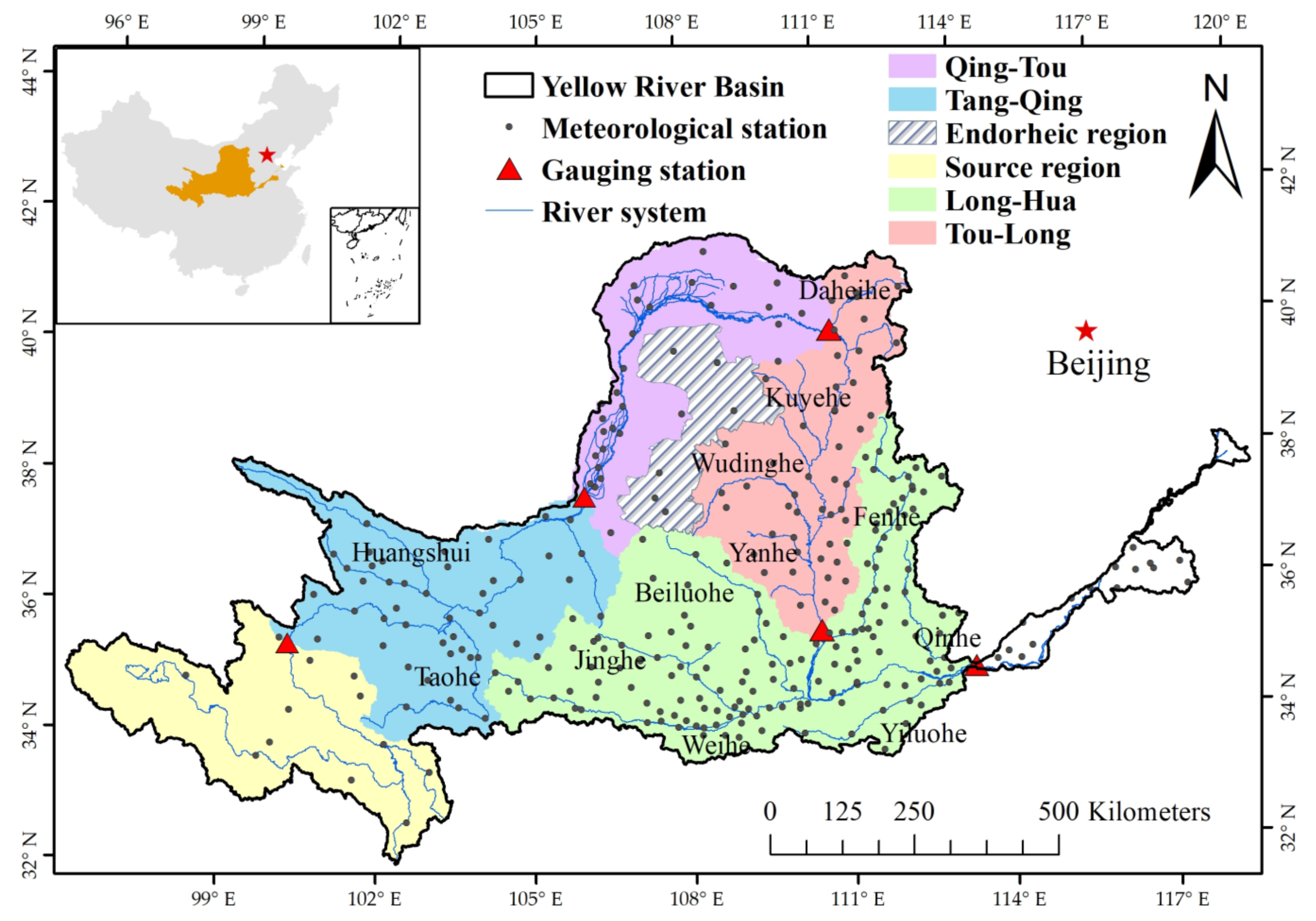
2.1. Study Area

The Yellow River is the second longest river in China, with a total length of 5464 km (Figure 1). Annual precipitation and annual average temperature over the YRB are 460 ± 165 mm and 7.2 ± 3.4 °C. The upper reaches of the YRB are the main source area of the river runoff, and the middle reaches are the main source area of the sediment. The multi-year average runoff volume and sediment discharge in the main river channel are 58 billion m3 and 1.6 billion tons, respectively. Historically, climate change and intense human activities have led to severe degradation of the ecosystem in the YRB. Therefore, major ecological restoration projects have been implemented in this area since 1999. The ecological environment and the capacity of the soil and water conservation have been significantly improved during the last two decades [35].

2.2. Data

In this study, five widely used global ET products were selected, including the GLDAS product, which is driven by three different land surface models (NOAH, VIC, and CLSM), the GLEAM_v3.3a product, and the PML_V2 product. In addition, the terrestrial water storage anomaly (TWSA) was derived from the average of the GRACE Jet Propulsion Laboratory (JPL) RL06_mascon and the Center for Space Research (CSR) RL06_mascon products. The global land surface satellite (GLASS) leaf area index (LAI) product was selected to characterize the vegetation structure parameter. Detailed information about these global products of the ecohydrological parameters is provided in Table 1.
The field observations of the precipitation, temperature, wind speed, sunshine duration, and relative humidity observed at the meteorological stations were obtained from the China Meteorological Data Service Centre (http://data.cma.cn/, accessed on 19 November 2021). The measured annual runoff measured at five major gauging stations (Tangnaihai, Qingtongxia, Toudaoguai, Longmen, and Huayuankou) located along the main river channel were obtained from the Hydrological Bureau of the Yellow River Conservancy Commission. Detailed information about these field measurements is provided in Table 2.
The ET or LAI product was downscaled by averaging the values of all pixels within a 0.25° grid. The GLDAS_VIC and GLDSA_CLSM products were upscaled to 0.25° using the nearest neighbor resampling method. All observations from the meteorological stations were spatially interpolated to a resolution of 0.25° using the AUSPLINE software. The VPD was calculated from the meteorological data using the method of Yuan et al. [36]. Finally, the daily meteorological data was averaged to the value at annual scale.
Table 1. Global products used in this study.
ParametersProductsSpatial ResolutionTemporal ResolutionTime DurationReference
ETGLDAS_NOAH0.25°monthly2000–2018Rodell et al. [11]
GLDAS_VIC2000–2018
GLDAS_CLSM2000–2018
GLEAM_v3.3a0.25°2000–2018Matens et al. [12]
PML_V2500 m8-day2000–2018Zhang et al. [9]
TWSAJPL RL06_mascon0.25°monthly2003–2018Wiese et al. [37]
CSR RL06_mascon0.25°monthly2003–2018Save et al. [38]
LAIGLASS1km8-day2000–2018Xiao et al. [39]
Table 2. Field observation datasets used in this study.
ParametersData SourcesNumber of SitesTemporal ResolutionTime Duration
Precipitation
Temperature
Wind speed
Sunshine duration
Relative humidity
China Meteorological Administration295daily2000–2018
Measured RunoffHydrological Bureau, Yellow River Water Conservancy Commission5yearly2000–2018

2.3. Method

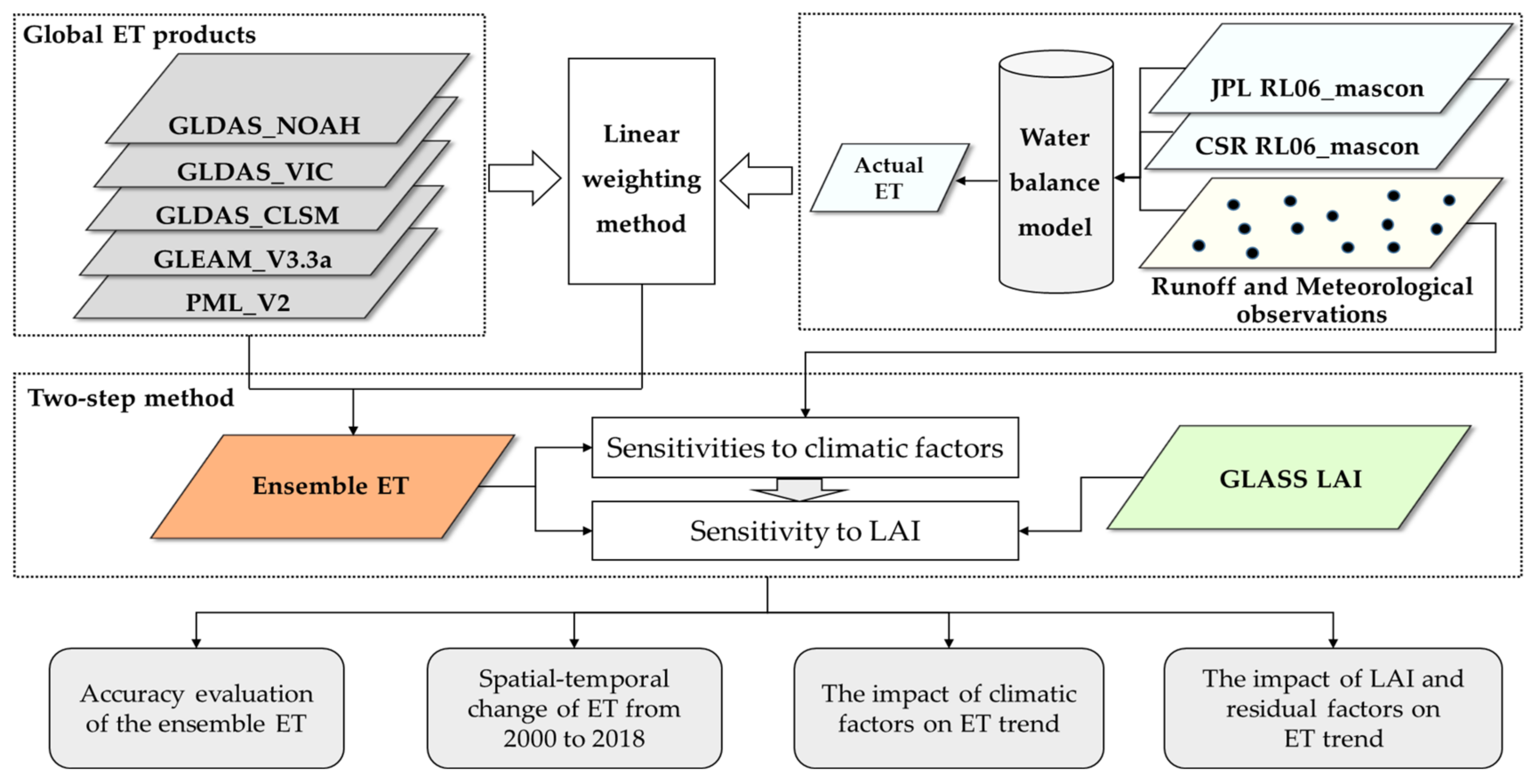
2.3.1. Overall Methodology

The overall flow scheme of attributing the evapotranspiration trend is shown in Figure 2. It includes the following major steps: (1) generate an ensemble ET in the YRB using a linear weighting method based on five global ET products and measured precipitation and runoff observations and GRACE products; (2) validate the ensemble ET with the regional ET calculated from the water balance principle; (3) explore the spatial-temporal change of ET from 2000 to 2018; (4) develop a “two-step” statistical regression strategy to derive sensitivity of the ET to climatic factors and LAI; and (5) evaluate the quantitative impacts of the climatic factors, vegetation, and residual factors on the ET trend.

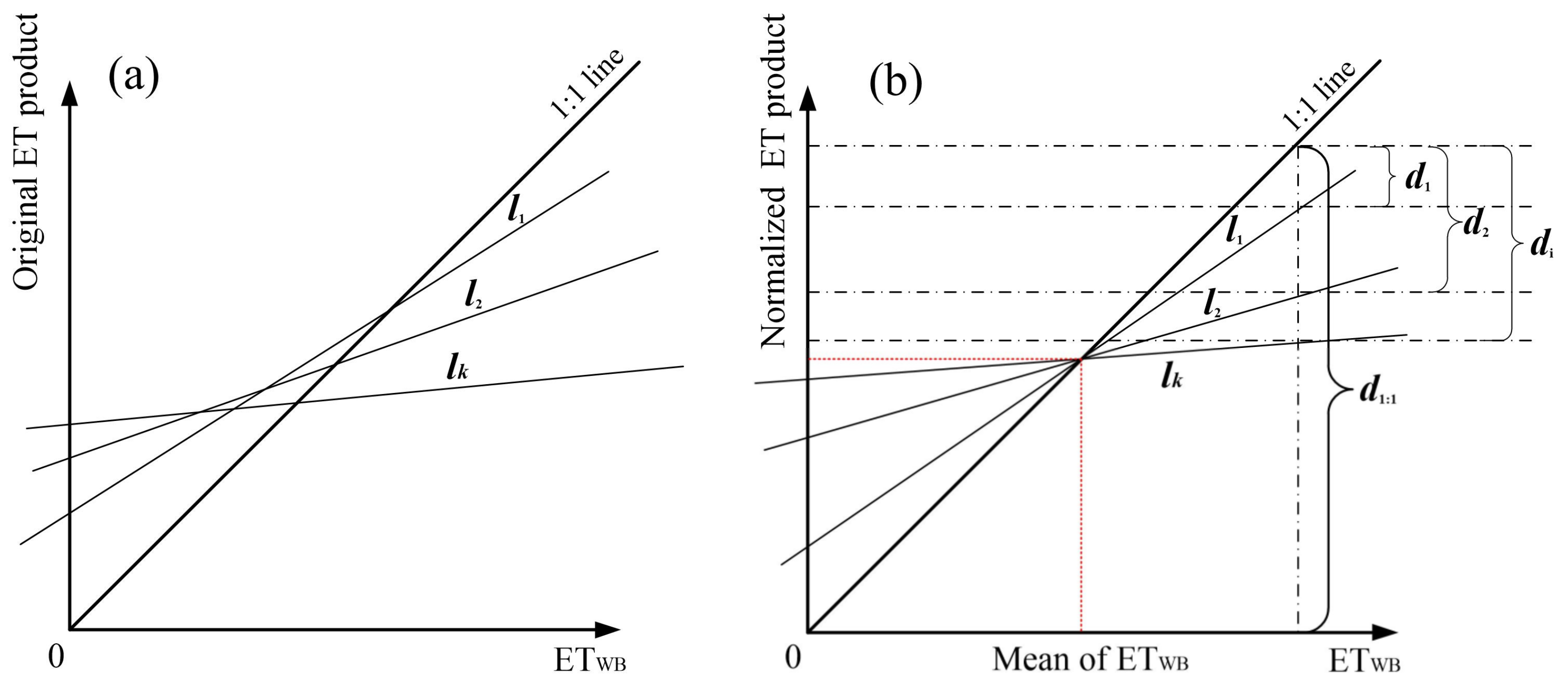
2.3.2. Ensemble ET derived using Linear Weighting Method

Since the shared database of the ET flux data is extremely limited in the YRB, and the effective observation range of the flux towers is much less than the spatial scale (0.25°) of most of the global ET products, it is not practical to assess the accuracies of the ET products in the YRB using the flux data. Therefore, based on previous studies that focused on areas with limited flux sites, the annual ET derived based on the water balance model was used as the field measurement at the regional scale [40].
A practical and easy-to-use linear weighting method [41] was employed to generate the ensemble estimates. The upper and middle reaches of the YRB were divided into five subregions, including the source region, Tangnaihai–Qingtongxia, Qingtongxia–Toudaoguai, Toudaoguai–Longmen, and Longmen–Huayuankou. The governing equation of the water balance model of each subregion is:
E T WB i j = P i j - R i j - Δ S i j
where E T WB i j is the spatially averaged ET of the jth sub-region in the ith year; Pij, Rij, and ΔSij are the measured precipitation (mm), runoff depth (mm), and the terrestrial water storage change (mm) derived from the TWSA in the jth subregion in the ith year, respectively.
ET estimates from each product was firstly normalized for each grid in each year using the following equation:
E T n o r m = E T + E T W B i j ¯ - E T i j ¯
where E T i j is the spatially averaged ET of the jth subregion in the ith year, and E T i j ¯ is the average of E T i j for the all subregions in all years. E T W B i j ¯ is the average of E T W B i j for the subregions in all years. ET represents the original ET product, and E T n o r m is normalized ET, and the average of E T n o r m for the all subregions in all years is equal to the E T W B i j ¯ .
V e n s e m b l e = k = 1 n w k × E T n o r m k
w k = f k / k = 1 n f k
f k = ( 1 - d k / d 1 : 1 ) × R k 2
where V e n s e m b l e is the ensemble ET, w k is the weight of kth normalized ET product, and n is the total number of ET products. Here, d1:1 represents the distance between the x axis ( E T W B ) and the 1:1 line, dk is the distance between line l k and the 1:1 line, and l k refers to the regression line between the E T W B and the E T n o r m k , as illustrated in the Figure 3 [41]. Thus, l k gives the following formula:
E T n o r m i j k = k k E T W B i j + b k
where k k is the regression coefficient, b k is a constant, and R k 2 is the determination coefficient of this regression model for the kth ET product. Thus, we further combine Equations (5) and (6) to obtain the following equations [41]:
f k = k k × R k 2 , 0 < k k 1 , 0 R k 2 1 1 k k × R k 2 , k k > 1 , 0 R k 2 1
In this study, we used the ET from odd-numbered years to calibrate the weight of different product, and the ET from even-numbered years were then used to validate the ensemble ET derived by a linear weighting method using the accuracy metrics of the root mean square error (RMSE), mean relative error (MRE) and relative RMSE (rRMSE).

2.3.3. Linear Slope Calculation

In this study, the slope of the linear regression model was used to characterize the annual rates of change of the different influencing factors and the ET. The slope was calculated as follows:
S l o p = n × i = 1 n i × X i i = 1 n i i = 1 n X i n × i = 1 n i 2 i = 1 n i 2

2.3.4. Quantitative Attribution Analysis Method for the ET Trend

Although commonly used detrended method can reduce the impact of interannual trends on overestimation of correlation between ET and climatic factors, this procedure can also inevitably underestimate the correlation between ET and LAI without obvious fluctuation characteristics. Therefore, a “two-step” scheme was developed to separately derive the sensitivity of ET to influencing factors.
Step 1:
We firstly calculated the sensitivity of ET to climatic factors with inherent fluctuating characteristics using detrended time-series data and multiple linear regression, as illustrated in the Equation (9):
d e _ E T = γ 0 + γ P C P N × d e _ P C P N + γ T e m p × d e _ T e m p + γ S D × d e _ S D + γ V P D × d e _ V P D + γ W S × d e _ W S
where de_ET, de_PCPN, de_Temp, de_SD, de_VPD, and de_WS are the detrended time-series of the PCPN, Temp, SD, VPD, and WS, respectively. γ P r e , γ T e m p , γ S D , γ V P D , and γ W S are the coefficients of regression model, and represent sensitivity of ET to these climatic factors, respectively (e.g., γ T e m p represents the ET change amount (mm) when Temp change per celsius degree).
Step 2:
Consequently, we calculated ET time-series (ETclimate) driven by the climatic factors using sensitivity calculated by Equation (9) and original time-series of climatic factors, as shown in the Equation (10). ET time-series (ETnon_climate) driven by the non-climatic factors was then derived using the Equation (11) and was employed to calculate the sensitivity of ET to LAI based on simple linear regression, as illustrated in the Equation (12).
E T climate = γ P C P N × P C P N + γ T e m p × T e m p + γ S D × S D + γ V P D × V P D + γ W S × W S
E T non _ climate = E T   -   E T climate
where PCPN, Temp, SD, VPD, and WS are the original time-series with trends of each climatic factor, ETclimate is the ET time-series driven by the climatic factors, and ETnon_climate is the ET time-series driven by the non-climatic factors.
E T non _ climate = γ 1 + γ L A I × L A I
where γ L A I is the sensitivity of the ET to the LAI, and LAI is the original time-series with a trend.
In this study, the ET trend was assumed to be the sum of the ET trend driven by the climatic factors (PCPN, Temp, SD, VPD, and WS), the LAI, and the residual factors. The differential form is as follow:
d E T d t = d E T P C P N d t + d E T T e m p d t + d E T S D d t + d E T V P D d t + d E T W S d t + d E T L A I d t + d E T R e s i . d t
where d E T d t   is the slope of the ET variation trend (mm/yr), and d E T P C P N d t ,   d E T T e m p d t ,   d E T S D d t ,   d E T V P D d t ,   d E T W S d t ,   d E T L A I d t , and d E T R e s i . d t are the impacts of PCPN, Temp, SD, VPD, WS, LAI, and the residual factors on the ET trend, respectively.
According to the basic concept of total differentiation, the impacts of the climatic factors and the LAI in Equation (13) can be decomposed via partial differentiation [30,31] as follows:
d E T d t = E T P C P N × d P C P N d t + E T T e m p × d T e m p d t + E T S D × d S D d t + E T V P D × d V P D d t + E T W S × d W S d t + E T L A I × d L A I d t + d E T R e s i . d t
where d P C P N d t , d T e m p d t ,   d S D d t , d V P D d t , d W S d t , and d L A I d t are the annual rates of change of PCPN, Temp, SD, VPD, WS, and LAI, respectively. E T P C P N , E T T e m p ,   E T S D , E T V P D , and E T W S are the sensitivity of ET to PCPN, Temp, SD, VPD, and WS, respectively, and they were calculated using Equation (9). E T L A I is the sensitivity of ET to LAI, which was calculated using Equation (12). d E T R e s i . d t is the residual in Equation (13).
The relative impact rate of each influencing factor on the ET trend was calculated using Equation (15).
C o n t r . X i = d E T X i d t i = 1 n d E T X i d t × 100 %
where C o n t r . X i is the relative impact rate of the ith influencing factor (PCPN, Temp, SD, VPD, WS, LAI, or residual factors) on the ET trend.

3. Results

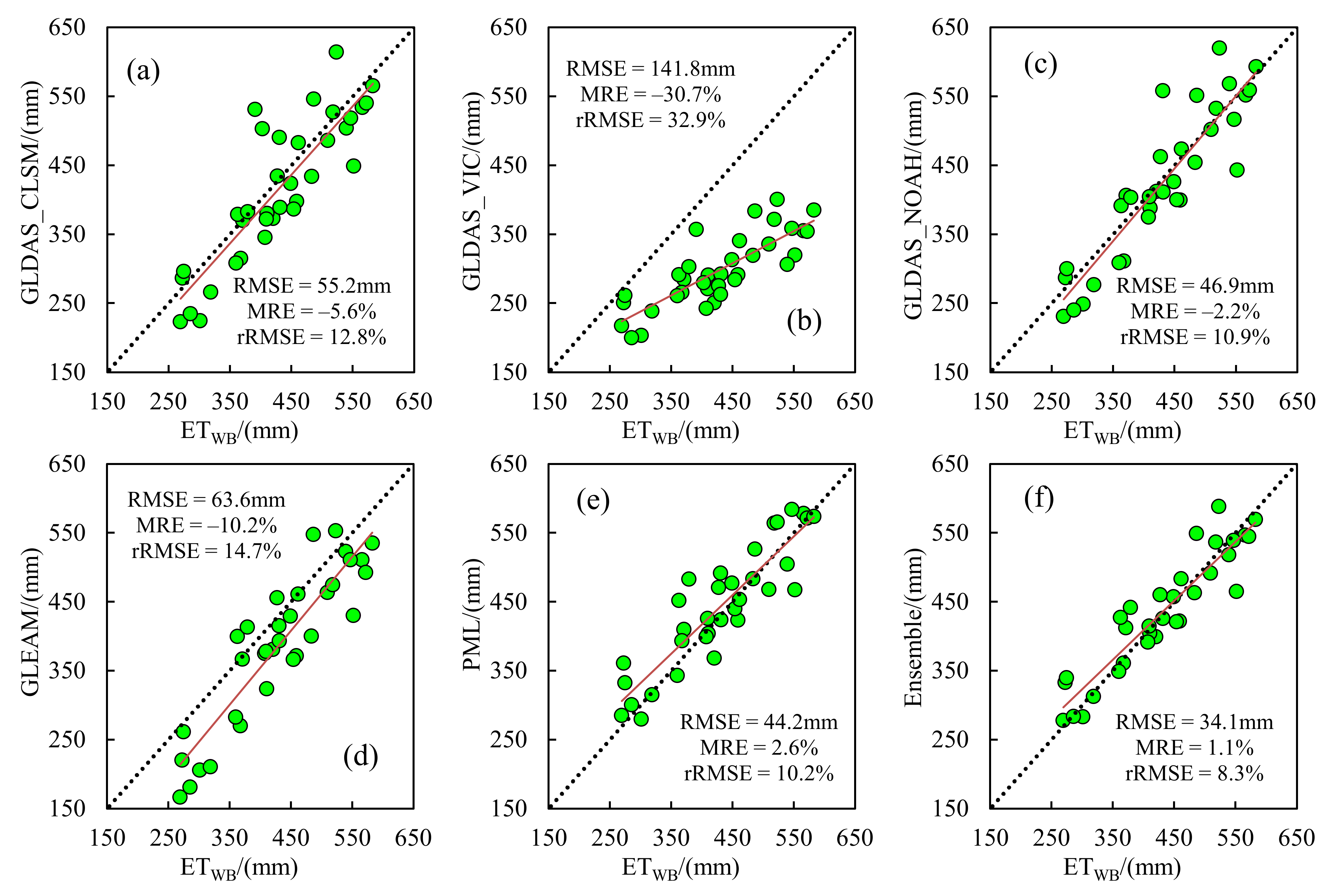
3.1. Accuracy Assessment of the Ensemble ET

The weight of each global ET products (GLDAS_CLSM, GLDAS_VIC, GLDAS_NOAH, GLEAM and PML) was calculated using Eqs.(3–5) respectively, and the ranking of weight of different ET products is PML (22%) > GLDAS_NOAH(22%) > GLDAS_CLSM (20%) > GLEAM (19%) > GLDAS_VIC (17%). This indicated that each selected ET product equally contributed to the merged product during the merging calculations.
The accuracies of the ET in the even-numbered years derived from five global ET products and the merged product were evaluated by E T WB , as illustrated in the Figure 4. The results showed that among the five ET products, the PML product had the highest accuracy (RMSE = 44.2 mm). Compared with the PML product, the accuracy metrics of ensemble ET (RMSE = 34.1mm, MRE = 1.1% and rRMSE = 8.3%) were improved. The results show that the ensemble ET could more accurately capture the spatial-temporal dynamics of ET in the YRB from 2000 to 2018.

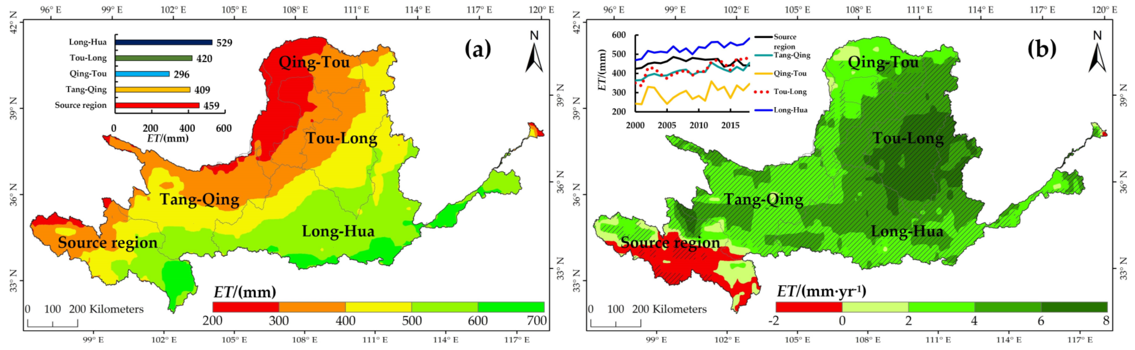
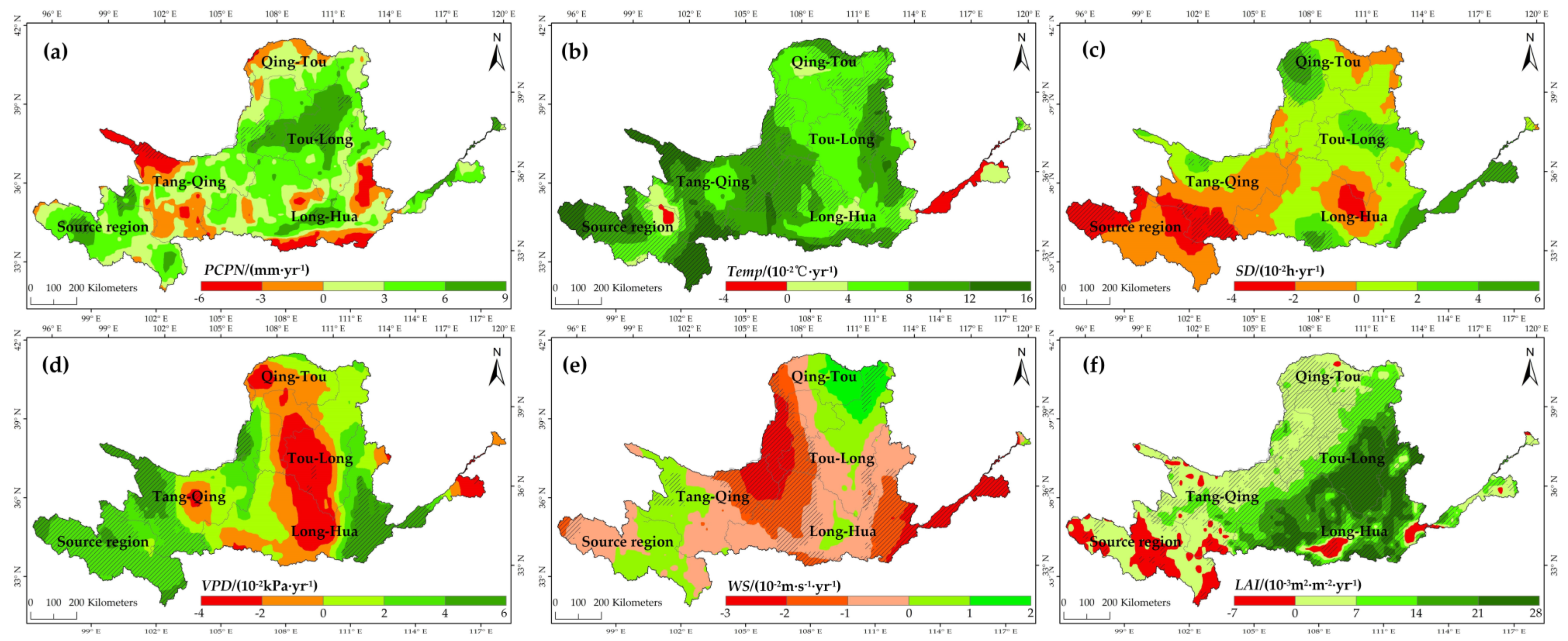
3.2. Spatial-Temporal Variation in ET and the Influencing Factors

Figure 5a illustrates the spatial distribution of the multi-year average ET from 2000 to 2018 in the YRB which yielded an average value 433 mm in the upper and middle regions. The spatial distribution of the ET was characterized by a gradual decrease from southeast to northwest. The Longmen–Huayuankou subregion had the highest multi-year average ET (529 mm), whereas the multi-year average ET of the Qingtongxia–Toudaoguai subregion was the lowest (296 mm).
The spatial distribution pattern of the interannual ET trend in the YRB from 2000 to 2018 is shown in Figure 5b. The overall ET trend in the upper and middle reaches of the YRB was 3.82 mm/yr. ET increased significantly in 77% of the study area, and the increase rate of Toudaoguai–Longmen subregion was >6 mm/yr. While ET decreased in only 7% of the study area, mainly distributed in the source area. It increased significantly from 2000 to 2006 and decreased slightly after 2007. The spatial distributions of the interannual trends of the climatic factors and the LAI in the YRB from 2000 to 2018 are shown in Figure 6.

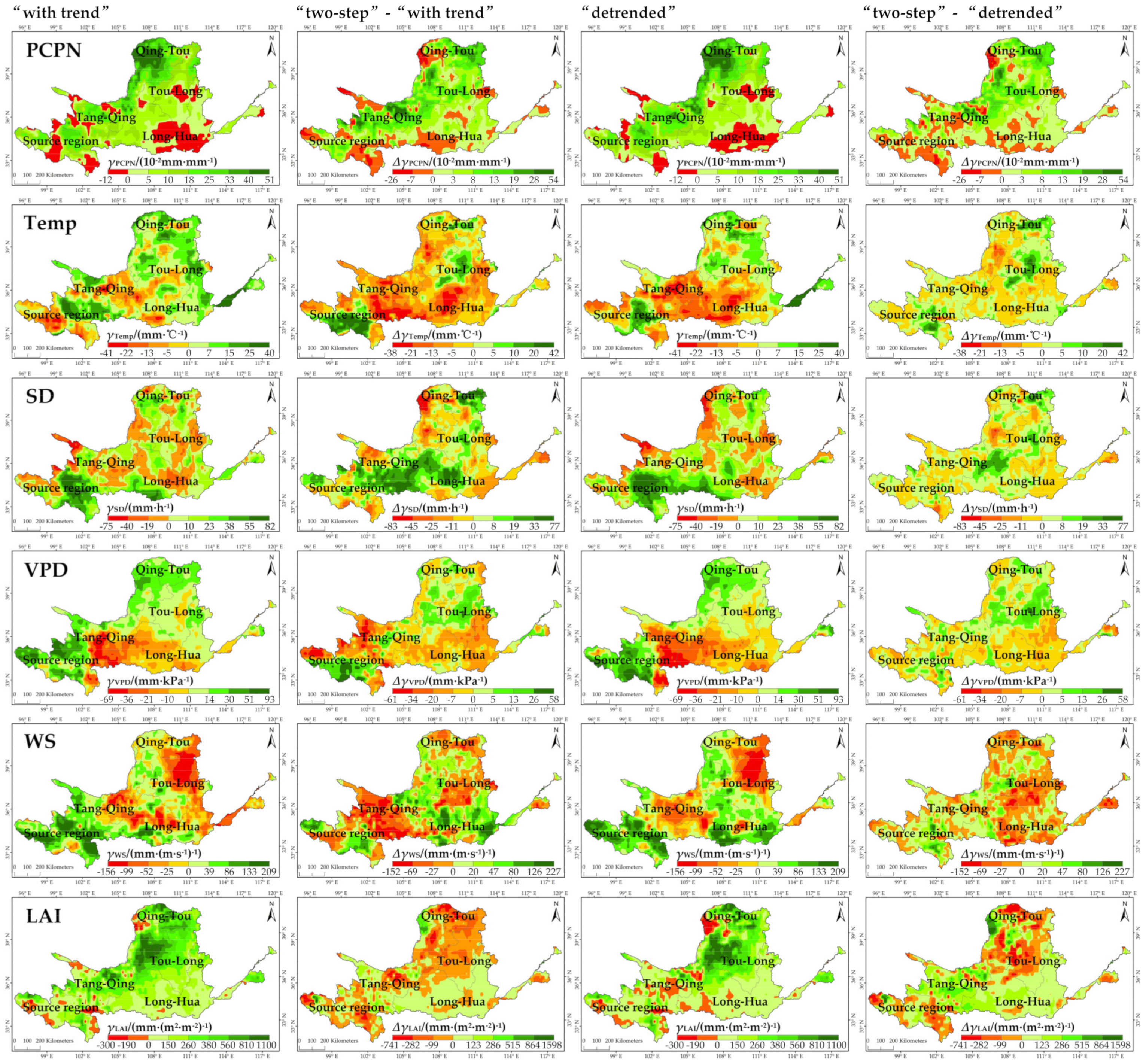
3.3. Spatial Pattern in the Sensitivity of the ET to the Influencing Factors

The spatial distributions of the sensitivity of the ET to climatic factors and the LAI are shown in Figure 7. The sensitivity of the ET to the PCPN ( γ P C P N ) exhibited an obvious spatial distribution, and γ P C P N decreased with increasing precipitation. The sensitivity of the ET to the temperature ( γ T e m p ) exhibited obvious spatial differences, and the regions with negative γ T e m p values were mainly concentrated in the western and southeastern parts of the source aera, the eastern part of the Tangnaihai–Qingtongxia subregion, and the western part of the Longmen–Huayuankou subregion, while the rest of the regions basically had positive γ T e m p . values. In most of the areas of the upper and middle reaches of the YRB, the sensitivity of the ET to the SD ( γ S D ) was positive, and the areas with negative γ S D values were mainly concentrated in the Huangshui River, Yiluohe River, and Fenhe River areas. The sensitivity of the ET to the VPD ( γ V P D ) had a spatial distribution similar to that of the γ T e m p , and the regions with positive γ V P D were mainly concentrated in the source area, the Qingtongxia–Toudaoguai subregion, and the Toudaoguai–Longmen subregion; while the rest of the regions had negative γ V P D . The negative sensitivity of the ET to the WS ( γ W S ) was mainly concentrated in the Tangnaihai–Qingtongxia subregion and the Toudaoguai–Longmen subregion, while the rest of the areas basically had positive γ W S values. The sensitivity of the ET to the LAI ( γ L A I ) was significantly higher in the arid areas than in wet areas, and γ L A I decreased with increasing precipitation.

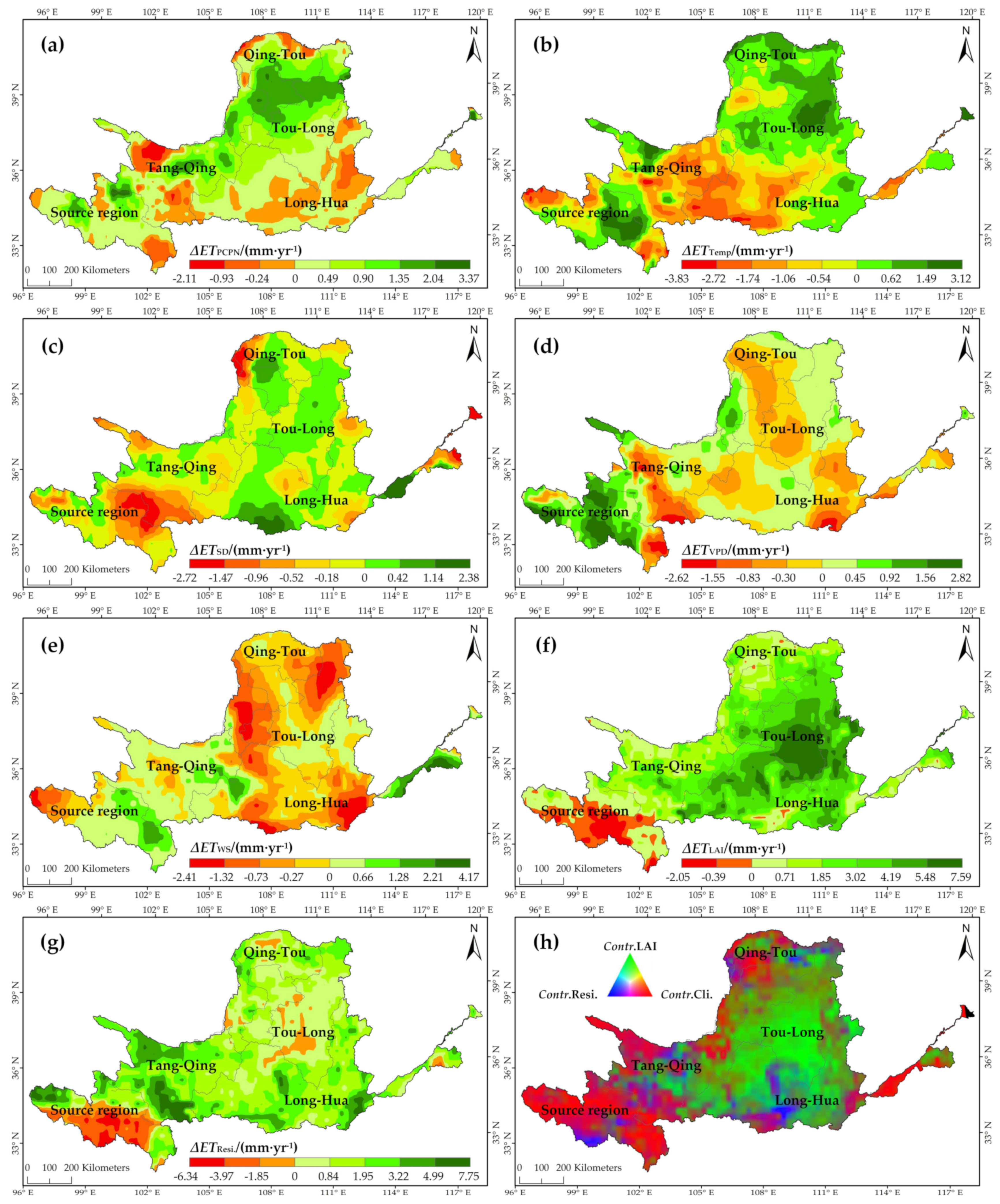
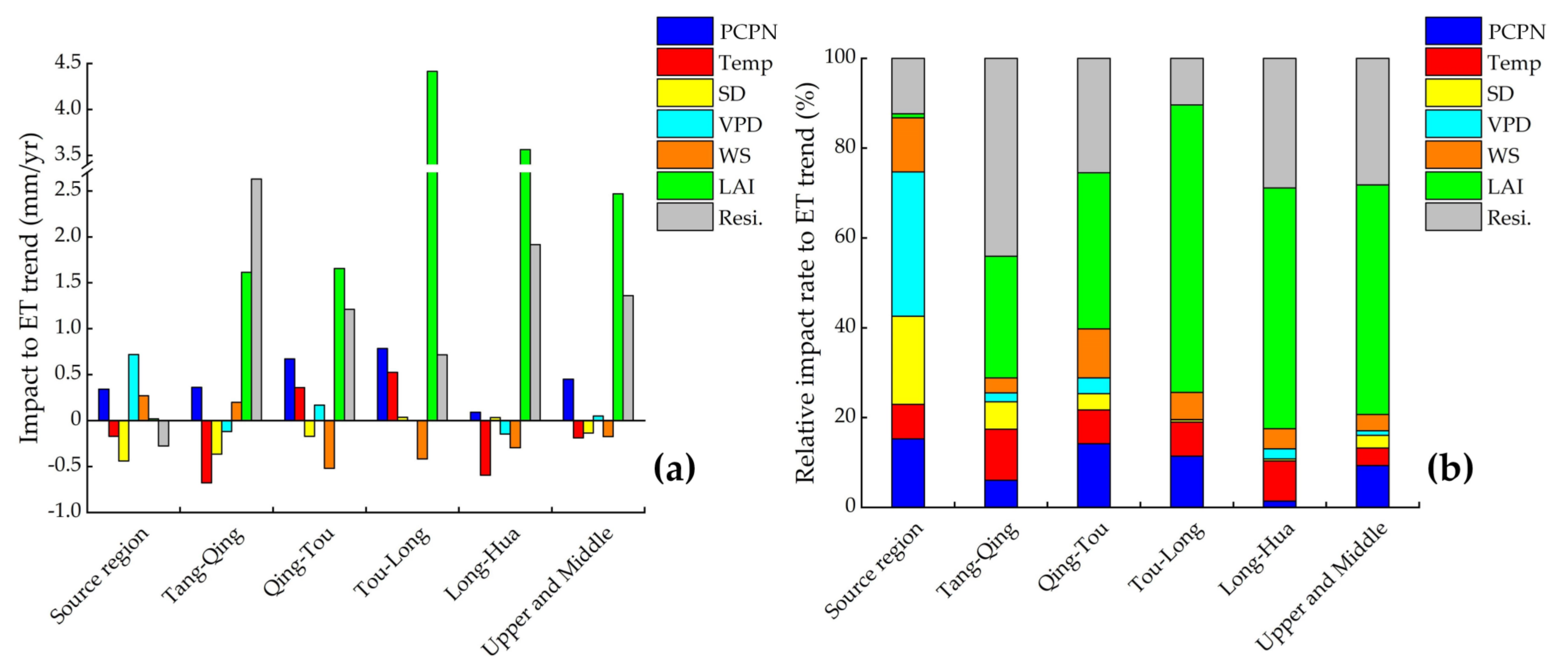
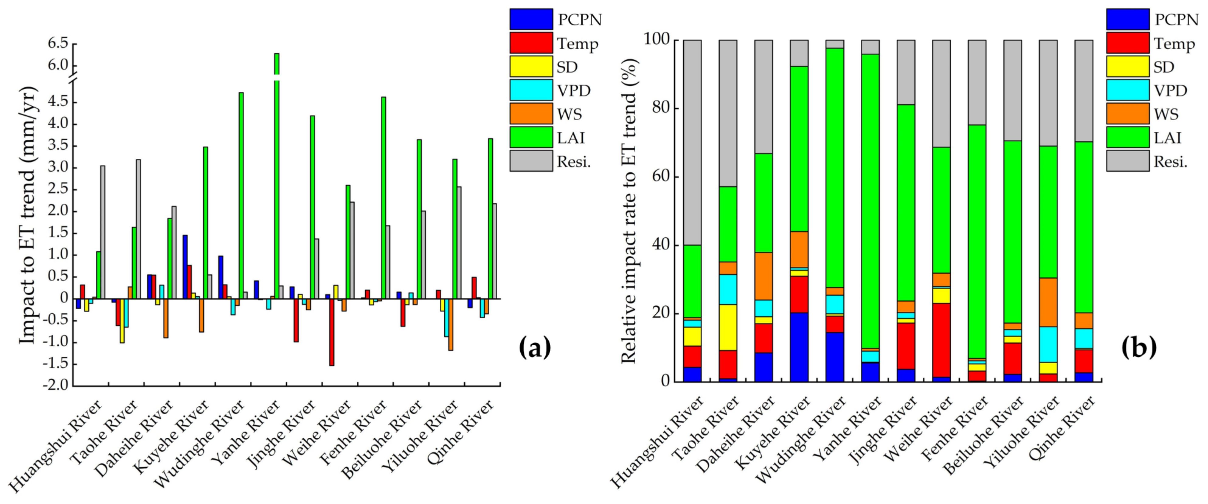
3.4. Impacts of the Influencing Factors on the ET Trend

The spatial distributions and statistics of the impacts of the different factors are shown in Figure 8a–g and Table 3. The areas with ET increased and decreased due to PCPN accounted for 75% and 25%, respectively, and the increasing and decreasing impacts of the PCPN on the ET trend (ΔETPCPN) were 0.68 mm/yr and −0.23 mm/yr, respectively. The areas in which the ET increased and decreased due to the Temp accounted for 50% and 50%, respectively, and the increasing and decreasing impacts of the Temp on the ET trend (ΔETTemp) were 0.64 mm/yr and −1 mm/yr, respectively. The ΔETTemp was positive in the central part of the source area and in most areas of the Qingtongxia–Longmen region. The ΔETTemp was negative in the most areas of Tangnaihai–Qingtongxia and Longmen–Huayuankou subregions. The areas with the ET increased and decreased due to the SD accounted for 40% and 60%, respectively, and the increasing and decreasing impacts of the SD on the ET trend (ΔETSD) were 0.19 mm/yr and −0.36 mm/yr, respectively. The lowest negative ΔETSD could be observed in the source region. The areas in which the ET increased and decreased due to the VPD accounted for 52% and 48%, respectively, and the increasing and decreasing impacts of the VPD on the ET trend (ΔETVPD) were 0.48 mm/yr and −0.41 mm/yr, respectively. The areas with the ET increased and decreased due to the WS accounted for 40% and 60%, respectively, and the increasing and decreasing impacts of the WS on the ET trend (ΔETWS) were 0.38 mm/yr and −0.55 mm/yr, respectively. The positive ΔETWS mainly occurred in most of the source area and in the Tangnaihai–Qingtongxia subregion; and the ΔETWS was negative in most of the Qingtongxia–Huayuankou region. The areas in which the ET increased and decreased due to the LAI accounted for 90% and 10%, respectively, and the increasing and decreasing impacts of the LAI on the ET trend (ΔETLAI) were 2.77 mm/yr and −0.35 mm/yr, respectively. The areas with the ET increased and decreased due to the residual factors accounted for 87% and 13%, respectively, and the increasing and decreasing impacts of the residual factors on the ET trend (ΔETResi.) were 1.82 mm/yr and −1.87 mm/yr, respectively. The ΔETResi. was positive in most areas of the YRB, and the negative ΔETResi. values were mainly distributed in the central part of the source area. An image of the relative impact rates of the climatic factors, LAI, and residual factors was synthesized using a Maxwell color triangle, which provided a more visual and objective view of the relative contribution of each factor to ET trend (Figure 8h).
The average impacts and relative impact rates of the different factors on the ET trend for different regions were calculated and are shown in Figure 9. Vegetation restoration was the dominant deriving factor for ET increase in the entire study area, with an impact of 2.47 mm/yr and a relative impact rate of 51.16% on the ET trend. The PCPN and VPD had increasing effects on the ET trend, with impacts of 0.45 mm/yr and 0.05 mm/yr, respectively. The Temp, SD, and WS had decreasing effects on the ET trend, with impacts of −0.19 mm/yr, −0.15 mm/yr, and −0.17 mm/yr, respectively. It should be noted that residual factors (e.g., changes in the microtopography and irrigation, etc.) cannot be ignored in affecting the ET trend, with a relatively great impact rate of 28.17%. Spatially, the ET trends of the Toudaoguai–Longmen and Longmen–Huayuankou subregions were dominated by the LAI, with impacts of 4.41 mm/yr and 3.56 mm/yr, respectively. The residual factors dominated the ET trend in the Tangnaihai–Qingtongxia subregion, with an impact of 2.63 mm/yr. The residual factors contributed more to the ET trend in the Longmen-Huayuankou subregion than in the Toudaoguai–Longmen subregion. The residual factors had a decreasing effect on the ET in the source area, with an impact of −0.28 mm/yr. The ET trends in the source area and the Qingtongxia–Toudaoguai subregion were dominated by the climatic factors. The climatic factors had the least effect on the ET trend in the Longmen–Huayuankou subregion (17.49%).
Further statistics on the average impacts and relative impact rates of the different factors on the ET trend in 12 typical subbasins are illustrated in Figure 10. The LAI is the dominant factor affecting the ET trend for subbasins in the middle reaches of the YRB, except for the Daheihe River where the vegetation increasing is not significant. The relative impact rates of LAI on ET trend were ranked as follows: Yanhe River > Wudinghe River > Fenhe River > Jinghe River > Beiluohe River > Qinhe River > Kuyehe River > Yiluohe River > Weihe River. The residual factors dominated the ET trend of the two rivers in the upper reaches of the YRB (Huangshui River and Taohe River), and the effect of the residual factors in the Huangshui River area was the largest (59.89%) among the selected subbasins. It should be noted that the climatic factors dominated the ET trend in the Daheihe River area, in which PCPN, Temp, and VPD had increasing effects on the ET trend, with impacts of 0.55 mm/yr, 0.54 mm/yr, and 0.31 mm/yr, respectively, while the SD and WS had decreasing effects on the ET trend, with impacts of −0.13 mm/yr and −0.89 mm/yr, respectively.

4. Discussion

4.1. Implications of the Sensitivity of the ET to the Influencing Factors Derived Using the “Two-Step” Scheme

In order to investigate the effects of the different statistical regression methods on deriving sensitivity of the ET to the influencing factors, the sensitivity of the ET to the influencing factors were calculated using multiple linear regression based on the original time-series data (“with trend” method) and the detrended time-series data (“detrended” method). The results derived from these two methods were compared with the proposed “two-step” method.
Figure 11 illustrates the sensitivity coefficients of the ET to the climatic factors obtained using the “two-step” method and the “detrended” method have similar spatial pattern, meanwhile, the sensitivity coefficients of the ET to the LAI by the “two-step” method and the “with trend” method have similar spatial distributions. This indicates that the “two-step” method can overcome the overestimation of sensitivity of ET to climatic factors associated with inherent fluctuating characteristics (precipitation, temperature, etc.) derived from “with trend” method and the underestimation of sensitivity of ET to influencing factors without fluctuation characteristics (vegetation structure, CO2 concentration, etc.) derived from “detrended” method.
We further calculated the differences in the impacts of the climatic factors, LAI, and residual factors on the ET trend using three methods, as shown in Table 4. It can be clearly seen that the “two-step” method is able to significantly reduce the impacts of climatic factors on the ET trend calculated by overestimated sensitivity using “with trend” method, and can significantly enhance the impact of LAI on the ET trend calculated by underestimated sensitivity using “detrended” method. According to the “detrended” method, vegetation greening is not the dominant factor for deriving ET trend in the YRB, which is inconsistent with most previous studies [32,33,42]. Meanwhile, Shao et al. [26] found the revegetation has led to a significant increase (4.39 mm/yr) in ET trend across the Loess Plateau during 2000–2015 based on the PT-JPL Model, which approximates to the impact (3.98 mm/yr) of vegetation on the ET trend in the middle reaches of YRB derived from the “two-step” method. In addition, according to the research of Zhang et al. [29], the impact of human activities (e.g., irrigation) on the ET trend in the YRB during 2003–2010 based on the measured runoff, soil moisture, and GRACE products was similar to the impact of residual factors derived from “two-step” method. These could be indirect evidence for demonstrating the improvement of “two-step” method on the impact assessment of influencing factors on the ET trend.

4.2. Underlying Causes of the Effects of the Influencing Factors on the ET Trend

In this study, the sensitivity coefficients of ET to climatic factors and vegetation were calculated separately using a simple statistical analysis method, and the impact of climatic factors and LAI on ET variations were finally quantitatively attributed. It was found that the ET trend in the upper and middle reaches of the YRB from 2000 to 2018 was 3.82 mm/yr, which is generally consistent with the findings of Bai et al. [43]. According to the Equation (14), it was known that the net ET trend can be decomposed into several impacts of different influencing factors on the ET trend, and the spatial pattern of impact of specific influencing factor on the ET trend was determined by the spatial pattern of change trend of influencing factor and the spatial pattern of sensitivity of ET to this factor. For example, if the signs of slope of PCPN trend and γPCPN are same, the impact of PCPN on the ET trend is positive (and vice versa). The spatial pattern of the ΔETPCPN and ΔETLAI were basically consistent with the spatial pattern of γPCPN and γLAI as a result of slopes of PCPN and LAI trend are positive in most areas. The spatial pattern of the ΔETtemp was basically same as the interannual trend of temp due to γtemp was positive over the whole study area. Although γSD is positive in most areas, there is negative trend of it in the source area, which led to the decreasing impact of SD to the ET trend. In the Loess Plateau, the combination of obvious decreasing trend of WS and positive γwind caused the decrease of ET trend. Except for source area, the factor of ‘resi.’ played an increasing role in the ET trend in other regions over the study area.
According to the previous studies, the precipitation influenced the evapotranspiration by increasing the soil water content and promoting plant growth in the water-limited regions [44,45,46]. The ΔETPCPN increased with the decreasing southeast-northwest precipitation gradient (Figure 8a), which was probably due to the rapid evaporation rate of the precipitation that was intercepted by the sparse vegetation canopy and infiltrated into the shallow soil in the arid region [47]. Therefore, the precipitation variability was the dominant factor controlling the evapotranspiration in the dryland ecosystems.
The spatial heterogeneity of impact of Temp on the ET trend (Figure 8b) can be explained by the fact that the low vegetation cover in the area where the soil evaporation was dominant and that the soil evaporation increased with increasing temperature. In contrast, in the high vegetation cover area, where the vegetation transpiration dominated the ET, the elevated temperature and drought stress physiologically reduced the vegetation photosynthesis and transpiration [48]. The higher SD meant more radiant energy, and evaporation was more likely to occur. While the SD changed the magnitude of the ET to some extent, the impact of the SD on the ET trend was lower in the arid and semi-arid regions compared to those of the other factors [22] (Figure 8c). The VPD was the degree of air dryness and, as the VPD increased, the vegetation transpiration became more intense. However, when the stomatal conductance decreases to a certain threshold, the vegetation transpiration is inhibited [36]. In recent years, the WS has been decreasing in the YRB, and the decrease in the WS will weaken the air flow and reduce the ET [32].
The vegetation mainly affects the ET through three ways: (1) vegetation increases can increase the vegetation interception evaporation [49,50]; (2) the vegetation can impede surface runoff, and developed roots can increase the soil infiltration rate, hence increasing the soil water content [51]; and (3) the changes in the vegetation transpiration and soil evaporation are directly affected by the changes in the soil water content, and the increase in the vegetation biomass can increase the vegetation transpiration and reduce the soil evaporation by shading the land [50]. The analysis of the combined effect of the vegetation on the ET shows that the increases in the vegetation transpiration and the vegetation interception evaporation were much larger than the decrease in the soil evaporation. The vegetation growth dominates the changes in the ET in biomes with higher canopy cover (e.g., agricultural fields, forests, and shrubs) [52,53].
The residual factors are also a significant driving force of the ET trend. Changes in the microtopography induced by terraces and check dams can effectively intercept surface runoff and increase the soil moisture, thus supplying sufficient water for vegetation growth and significantly increasing the vegetation transpiration, soil evaporation, and surface water evaporation [54,55]. In addition, irrigation can significantly increase the soil evaporation and transpiration of corps. The decreasing impacts of the residual factors on the ET trend in the source area may be due to the improved water storage capacity of the underlying surface caused by thawing of the permafrost [56]. The impacts of the residual factors in the Tangnaihai–Qingtongxia and Longmen–Huayuankou subregions were relatively high, indicating that the human activities, including soil and water conservation measures and irrigation, were more intensive in these regions [29].

4.3. Impact on Water Yield Change Trend at the Subregion Scale

The continuous increase in the actual evapotranspiration directly affects the water supply to the ecosystem in the YRB. Based on the principle of water balance, combined with the merged ET product and measured precipitation data, the trends of the water yield (P-ET) in the different subregions were calculated (Table 5).
Since the 21st century, the annual precipitation trend in the YRB has been insignificant (Figure 6a), and the actual annual evapotranspiration has increased significantly (Figure 5b), resulting in a decrease in the water yield of basin. The source area of the YRB was affected by the increased precipitation, and the water resource supply increased. In contrast, the trend of the water yield in the Loess Plateau region has decreased, and the regional drought has intensified. The Loess Plateau region is one of the main areas where ecological restoration projects have been implemented in China. During 1999–2013, the vegetation coverage in the Loess Plateau region increased from 31.6% to 59.6% due to the implementation of the reforestation project [15]. Afforestation can enhance the ecological service functions of a regional ecosystem, including carbon sequestration, oxygen release, and soil and water conservation, but it can also weaken the water supply capacity of the regional ecosystem [45]. Fast-growing anthropogenic forests have a greater evapotranspiration capacity than natural forests [33]. Indeed, the forest-dominated areas in the YRB have been suffering from increased drought in recent decades [57]. Deep-rooted trees are more prone to severe soil desiccation than shallow-rooted vegetation such as grasses [58]. Under the background of intensifying regional drought, it was recommended that one gives priority to strengthening the protection of the local native vegetation during the ecological protection and restoration in the arid areas of the YRB. Moreover, in afforestation and reforestation projects, tree species with weaker transpiration capacities should be selected to reduce the water consumption of the vegetation and mitigate the trend of intensifying drought.

4.4. Uncertainties

In this study, the ETWB calculated by the water balance equation based on the measured runoff and rainfall data and GRACE products was taken to be the ET measurement at the regional scale. It should be noted that Blazquez et al. [59] found that the geocenter motion and glacial isostatic adjustment corrections dominate the uncertainty in GRACE estimate of the global water budget, and their contribution to the uncertainty in GRACE estimate is ±0.21 and ±0.12 mm yr−1, respectively. These uncertainties from the GRACE product could affect the accuracy of ETWB. However, the average of two GRACE products has a reduced uncertainty to some extent. Martens et al. [12] also found that the average correlations against global eddy-covariance measurements in a range between 0.78 and 0.81 for the GLEAM products with different version. PML_V2 ET product was evaluated against eight-day measurements at global 95 widely-distributed flux towers for 10 plant functional types, with a RMSE and Bias of 0.69 mm d−1 and −1.8% [9]. The uncertainties of hydrological fluxes from GLDAS are affected by the different meteorological data sets and land surface models [11]. Therefore, the uncertainties existed in the global ET products used in this study would inevitably affect the attributing results of ET trend. The sensitivity of the ET to the influencing factors were calculated using the multiple regression method under the assumptions that there were no interactions between the different influencing factors and the ET has linear responses to these influencing factors. These assumptions also contribute to some uncertainties. Since the biophysical and biochemical feedbacks of the underlying surface changes to the atmosphere were not considered, the attribution results in this study only reflect the direct impacts of the different influencing factors on the ET trend. Moreover, the impact of residual factors on the ET trend inevitably contained some uncertainties from the simulation error of multivariate regression model.
Therefore, the present study requires further investigations. Sufficient precipitation, runoff, soil moisture, and ET measurement datasets should be collected in the YRB, and a combination of nonlinear statistical models, remote sensing models, and hydrological models should be employed to comprehensively evaluate the impacts of the different influencing factors on the ET trend and their spatial patterns in order to reduce the uncertainties caused by using different datasets and analysis methods. In addition, the effects of the biophysical and biochemical feedbacks of the underlying surface changes to the atmosphere on the variation in the ET should be further discussed in the future.

5. Conclusions

In this study, five global ET products were merged by a linear weighting method. It is demonstrated that the ensemble ET can utilize the advantages of each individual ET product to improve the accuracy of ET simulation at reginal scale. Based on the ensemble ET, the responses of spatial-temporal variation of ET trend to the climatic factors, LAI, and residual factors from 2000 to 2018 were explored using three different easy-to-use statistical methods. It was found that different statistical method would bring relatively great uncertainties for the sensitivity of ET to influencing factors, which inevitably led to divergent spatial pattern of estimated impacts of influencing factors on the ET trend. By comparing the results from different statistical methods, the proposed “two-step” method can improve the sensitivity of ET to influencing factors. Therefore, uncertainties for the impact assessment of climatic factors and vegetation could be reduced. The attributing analysis demonstrated that interannual trend of ET in the upper and middle reaches of the YRB was 3.82 mm/yr. This trend was dominantly controlled by the vegetation greening, with an impact of 2.47 mm/yr and a relative impact rate of 51.16%. It should not be neglected for the impact of the residual factors on the ET trend mainly induced by the microtopography, irrigation, etc. with an impact of 1.36 mm/yr and a relative impact rate of 28.17%. The PCPN and VPD had increasing effects on the ET trend, with impacts of 0.45 mm/yr and 0.05 mm/yr, respectively. However, the variations in the Temp, SD, and WS had decreasing effects on the ET trend, with impacts of –0.19 mm/yr, −0.15 mm/yr, and −0.17 mm/yr, respectively.

Author Contributions

All authors contributed to the design and development of this manuscript. Z.C. performed the data processing and wrote the first draft of the manuscript. Z.W. gave constructive suggestions on the design and modification of the manuscript. T.H. and Q.T. also helped process the data in this paper. P.X., L.W. and P.Z. helped edit the manuscript prior to submission. All authors have read and agreed to the published version of the manuscript.

Funding

This research was funded by the National Natural Science Foundation of China (41701509), Young Elite Scientist Sponsorship by CAST (2017QNRC023), and Special Research Fund of the YRIHR (HKY-JBYW-2020-09).

Data Availability Statement

The data presented in this study are available on request from the corresponding author for research purposes.

Acknowledgments

We gratefully thank the anonymous reviewers for their critical comments and constructive suggestions on the manuscript.

Conflicts of Interest

The authors declare no conflict of interest.

References

  1. Zhang, Y.; Leuning, R.; Hutley, L.B.; Beringer, J.; McHugh, I.; Walker, J.P. Using long-term water balances to parameterize surface conductances and calculate evaporation at 0.05° spatial resolution. Water Resour. Res. 2010, 46. [Google Scholar] [CrossRef] [Green Version]
  2. Liu, S.M.; Xu, Z.W.; Zhu, Z.L.; Jia, Z.Z.; Zhu, M.J. Measurements of evapotranspiration from eddy-covariance systems and large aperture scintillometers in the Hai River Basin, China. J. Hydrol. 2013, 487, 24–38. [Google Scholar] [CrossRef]
  3. Vinukollu, R.K.; Wood, E.F.; Ferguson, C.R.; Fisher, J.B. Global estimates of evapotranspiration for climate studies using multi-sensor remote sensing data: Evaluation of three process-based approaches. Remote Sens. Environ. 2011, 115, 801–823. [Google Scholar] [CrossRef]
  4. Tian, F.; Qiu, G.; Yang, Y.; Lü, Y.; Xiong, Y. Estimation of evapotranspiration and its partition based on an extended three-temperature model and MODIS products. J. Hydrol. 2013, 498, 210–220. [Google Scholar] [CrossRef]
  5. Ma, Y.-J.; Li, X.-Y.; Liu, L.; Yang, X.-F.; Wu, X.-C.; Wang, P.; Lin, H.; Zhang, G.-H.; Miao, C.-Y. Evapotranspiration and its dominant controls along an elevation gradient in the Qinghai Lake watershed, northeast Qinghai-Tibet Plateau. J. Hydrol. 2019, 575, 257–268. [Google Scholar] [CrossRef]
  6. Ramoelo, A.; Majozi, N.; Mathieu, R.; Jovanovic, N.; Nickless, A.; Dzikiti, S. Validation of global evapotranspiration product (MOD16) using flux tower data in the African savanna, South Africa. Remote Sens. 2014, 6, 7406–7423. [Google Scholar] [CrossRef] [Green Version]
  7. Jung, M.; Reichstein, M.; Ciais, P.; Seneviratne, S.I.; Sheffield, J.; Goulden, M.L.; Bonan, G.; Cescatti, A.; Chen, J.; de Jeu, R.; et al. Recent decline in the global land evapotranspiration trend due to limited moisture supply. Nature 2010, 467, 951–954. [Google Scholar] [CrossRef]
  8. Mu, Q.; Zhao, M.; Running, S.W. Improvements to a MODIS global terrestrial evapotranspiration algorithm. Remote Sens. Environ. 2011, 115, 1781–1800. [Google Scholar] [CrossRef]
  9. Zhang, Y.; Kong, D.; Gan, R.; Chiew, F.H.S.; McVicar, T.R.; Zhang, Q.; Yang, Y. Coupled estimation of 500 m and 8-day resolution global evapotranspiration and gross primary production in 2002–2017. Remote Sens. Environ. 2019, 222, 165–182. [Google Scholar] [CrossRef]
  10. Kobayashi, S.; Ota, Y.; Harada, Y.; Ebita, A.; Moriya, M.; Onoda, H.; Onogi, K.; Kamahori, H.; Kobayashi, C.; Endo, H.; et al. The JRA-55 reanalysis: General specifications and basic characteristics. J. Meteorol. Soc. Jpn. Ser. II 2015, 93, 5–48. [Google Scholar] [CrossRef] [Green Version]
  11. Rodell, M.; Houser, P.; Jambor, U.; Gottschalck, J.; Mitchell, K.; Meng, C.-J.; Arsenault, K.; Cosgrove, B.; Radakovich, J.; Bosilovich, M. The global land data assimilation system. Bull. Am. Meteorol. Soc. 2004, 85, 381–394. [Google Scholar] [CrossRef] [Green Version]
  12. Martens, B.; Miralles, D.G.; Lievens, H.; van der Schalie, R.; de Jeu, R.A.M.; Fernández-Prieto, D.; Beck, H.E.; Dorigo, W.A.; Verhoest, N.E.C. GLEAM v3: Satellite-based land evaporation and root-zone soil moisture. Geosci. Model. Dev. 2017, 10, 1903–1925. [Google Scholar] [CrossRef] [Green Version]
  13. Liu, F.; Chen, S.; Peng, J.; Chen, G. Temporal variability of water discharge and sediment load of the Yellow River into the sea during 1950–2008. J. Geogr. Sci. 2011, 21, 1047–1061. [Google Scholar] [CrossRef]
  14. Yin, Y.; Tang, Q.; Liu, X.; Zhang, X. Water scarcity under various socio-economic pathways and its potential effects on food production in the Yellow River basin. Hydrol. Earth Syst. Sci. 2017, 21, 791–804. [Google Scholar] [CrossRef] [Green Version]
  15. Chen, Y.; Wang, K.; Lin, Y.; Shi, W.; Song, Y.; He, X. Balancing green and grain trade. Nat. Geosci. 2015, 8, 739–741. [Google Scholar] [CrossRef]
  16. Hua, F.; Wang, X.; Zheng, X.; Fisher, B.; Wang, L.; Zhu, J.; Tang, Y.; Yu, D.W.; Wilcove, D.S. Opportunities for biodiversity gains under the world’s largest reforestation programme. Nat. Commun. 2016, 7, 12717. [Google Scholar] [CrossRef] [PubMed] [Green Version]
  17. Wang, W.; Zhang, Y.; Tang, Q. Impact assessment of climate change and human activities on streamflow signatures in the Yellow River Basin using the Budyko hypothesis and derived differential equation. J. Hydrol. 2020, 591, 125460. [Google Scholar] [CrossRef]
  18. Jia, X.; Shao, M.A.; Zhu, Y.; Luo, Y. Soil moisture decline due to afforestation across the Loess Plateau, China. J. Hydrol. 2017, 546, 113–122. [Google Scholar] [CrossRef]
  19. Cai, X.; Rosegrant, M.W. Optional water development strategies for the Yellow River Basin: Balancing agricultural and ecological water demands. Water Resour. Res. 2004, 40, 1–11. [Google Scholar] [CrossRef] [Green Version]
  20. Gao, G.; Chen, D.; Xu, C.-Y.; Simelton, E. Trend of estimated actual evapotranspiration over China during 1960–2002. J. Geophys. Res. Atmos. 2007, 112. [Google Scholar] [CrossRef] [Green Version]
  21. Goyal, R.K. Sensitivity of evapotranspiration to global warming: A case study of arid zone of Rajasthan (India). Agric. Water Manag. 2004, 69, 1–11. [Google Scholar] [CrossRef]
  22. Li, T.; Xia, J.; Zhang, L.; She, D.; Wang, G.; Cheng, L. An improved complementary relationship for estimating evapotranspiration attributed to climate change and revegetation in the Loess Plateau, China. J. Hydrol. 2021, 592, 125516. [Google Scholar] [CrossRef]
  23. Zha, T.; Li, C.; Kellomäki, S.; Peltola, H.; Wang, K.-Y.; Zhang, Y. Controls of evapotranspiration and CO2 fluxes from Scots pine by surface conductance and abiotic factors. PLoS ONE 2013, 8, e69027. [Google Scholar] [CrossRef] [Green Version]
  24. Burn, D.H.; Hesch, N.M. Trends in evaporation for the Canadian Prairies. J. Hydrol. 2007, 336, 61–73. [Google Scholar] [CrossRef]
  25. Shen, M.; Piao, S.; Jeong, S.-J.; Zhou, L.; Zeng, Z.; Ciais, P.; Chen, D.; Huang, M.; Jin, C.-S.; Li, L.Z.X.; et al. Evaporative cooling over the Tibetan Plateau induced by vegetation growth. Proc. Natl. Acad. Sci. USA 2015, 112, 9299. [Google Scholar] [CrossRef] [Green Version]
  26. Shao, R.; Zhang, B.; Su, T.; Long, B.; Cheng, L.; Xue, Y.; Yang, W. Estimating the increase in regional evaporative water consumption as a result of vegetation restoration over the Loess plateau, China. J. Geophys. Res. Atmos. 2019, 124, 11783–11802. [Google Scholar] [CrossRef]
  27. Qiu, L.; Wu, Y.; Shi, Z.; Chen, Y.; Zhao, F. Quantifying the responses of evapotranspiration and its components to vegetation restoration and climate change on the Loess plateau of China. Remote Sens. 2021, 13, 2358. [Google Scholar] [CrossRef]
  28. Lv, X.; Zuo, Z.; Sun, J.; Ni, Y.; Wang, Z. Climatic and human-related indicators and their implications for evapotranspiration management in a watershed of Loess plateau, China. Ecol. Indic. 2019, 101, 143–149. [Google Scholar] [CrossRef]
  29. Zhang, M.; Yuan, X. Crucial role of natural processes in detecting human influence on evapotranspiration by multisource data analysis. J. Hydrol. 2020, 580, 124350. [Google Scholar] [CrossRef]
  30. Li, G.; Zhang, F.; Jing, Y.; Liu, Y.; Sun, G. Response of evapotranspiration to changes in land use and land cover and climate in China during 2001–2013. Sci. Total Environ. 2017, 596–597, 256–265. [Google Scholar] [CrossRef] [PubMed]
  31. Yang, L.; Feng, Q.; Adamowski, J.F.; Alizadeh, M.R.; Zhu, M. The role of climate change and vegetation greening on the variation of terrestrial evapotranspiration in northwest China’s Qilian Mountains. Sci. Total Environ. 2020, 759, 143532. [Google Scholar] [CrossRef]
  32. Jiang, Z.-Y.; Yang, Z.-G.; Zhang, S.-Y.; Liao, C.-M.; Hu, Z.-M.; Cao, R.-C.; Wu, H.-W. Revealing the spatio-temporal variability of evapotranspiration and its components based on an improved Shuttleworth-Wallace model in the Yellow River Basin. J. Environ. Manag. 2020, 262, 110310. [Google Scholar] [CrossRef]
  33. Pei, T.; Wu, X.; Li, X.; Zhang, Y.; Shi, F.; Ma, Y.; Wang, P.; Zhang, C. Seasonal divergence in the sensitivity of evapotranspiration to climate and vegetation growth in the Yellow River Basin, China. J. Geophys. Res. Biogeosci. 2017, 122, 103–118. [Google Scholar] [CrossRef]
  34. Zhou, L.; Tucker, C.J.; Kaufmann, R.K.; Slayback, D.; Shabanov, N.V.; Myneni, R.B. Variations in northern vegetation activity inferred from satellite data of vegetation index during 1981 to 1999. J. Geophys. Res. Atmos. 2001, 106, 20069–20083. [Google Scholar] [CrossRef]
  35. Li, J.; Peng, S.; Li, Z. Detecting and attributing vegetation changes on China s Loess Plateau. Agric. For. Meteorol. 2017, 247, 260–270. [Google Scholar] [CrossRef]
  36. Yuan, W.; Zheng, Y.; Piao, S.; Ciais, P.; Lombardozzi, D.; Wang, Y.; Ryu, Y.; Chen, G.; Dong, W.; Hu, Z.; et al. Increased atmospheric vapor pressure deficit reduces global vegetation growth. Sci. Adv. 2019, 5, eaax1396. [Google Scholar] [CrossRef] [PubMed] [Green Version]
  37. Wiese, D.N.; Landerer, F.W.; Watkins, M.M. Quantifying and reducing leakage errors in the JPL RL05M GRACE mascon solution. Water Resour. Res. 2016, 52, 7490–7502. [Google Scholar] [CrossRef]
  38. Save, H.; Bettadpur, S.; Tapley, B.D. High-resolution CSR GRACE RL05 mascons. J. Geophys. Res. Solid Earth 2016, 121, 7547–7569. [Google Scholar] [CrossRef]
  39. Xiao, Z.; Liang, S.; Wang, J.; Chen, P.; Yin, X.; Zhang, L.; Song, J. Use of general regression neural networks for generating the GLASS leaf area index product from time-series MODIS surface reflectance. IEEE Trans. Geosci. Remote Sens. 2014, 52, 209–223. [Google Scholar] [CrossRef]
  40. Wan, Z.; Zhang, K.; Xue, X.; Hong, Z.; Hong, Y.; Gourley, J.J. Water balance-based actual evapotranspiration reconstruction from ground and satellite observations over the conterminous United States. Water Resour. Res. 2015, 51, 6485–6499. [Google Scholar] [CrossRef]
  41. Yao, Y.; Liang, S.; Xie, X.; Cheng, J.; Jia, K.; Li, Y.; Liu, R. Estimation of the terrestrial water budget over northern China by merging multiple datasets. J. Hydrol. 2014, 519, 50–68. [Google Scholar] [CrossRef]
  42. Xu, S.; Yu, Z.; Yang, C.; Ji, X.; Zhang, K. Trends in evapotranspiration and their responses to climate change and vegetation greening over the upper reaches of the Yellow River Basin. Agric. For. Meteorol. 2018, 263, 118–129. [Google Scholar] [CrossRef]
  43. Bai, M.; Mo, X.; Liu, S.; Hu, S. Contributions of climate change and vegetation greening to evapotranspiration trend in a typical hilly-gully basin on the Loess Plateau, China. Sci. Total Environ. 2019, 657, 325–339. [Google Scholar] [CrossRef] [PubMed]
  44. Liu, Q.; Yang, Z. Quantitative estimation of the impact of climate change on actual evapotranspiration in the Yellow River Basin, China. J. Hydrol. 2010, 395, 226–234. [Google Scholar] [CrossRef]
  45. Villarreal, S.; Vargas, R.; Yepez, E.A.; Acosta, J.S.; Castro, A.; Escoto-Rodriguez, M.; Lopez, E.; Martínez-Osuna, J.; Rodriguez, J.C.; Smith, S.V.; et al. Contrasting precipitation seasonality influences evapotranspiration dynamics in water-limited shrublands. J. Geophys. Res. Biogeosci. 2016, 121, 494–508. [Google Scholar] [CrossRef] [Green Version]
  46. Feng, K.; Siu, Y.L.; Guan, D.; Hubacek, K. Assessing regional virtual water flows and water footprints in the Yellow River Basin, China: A consumption based approach. Appl. Geogr. 2012, 32, 691–701. [Google Scholar] [CrossRef]
  47. Heitman, J.L.; Horton, R.; Sauer, T.J.; DeSutter, T.M. Sensible heat observations reveal soil-water evaporation dynamics. J. Hydrometeorol. 2008, 9, 165–171. [Google Scholar] [CrossRef] [Green Version]
  48. Cai, X. Water stress, water transfer and social equity in Northern China—Implications for policy reforms. J. Environ. Manag. 2008, 87, 14–25. [Google Scholar] [CrossRef]
  49. Deng, C.; Zhang, B.; Cheng, L.; Hu, L.; Chen, F. Vegetation dynamics and their effects on surface water-energy balance over the Three-North Region of China. Agric. For. Meteorol. 2019, 275, 79–90. [Google Scholar] [CrossRef]
  50. Williams, I.N.; Torn, M.S. Vegetation controls on surface heat flux partitioning, and land-atmosphere coupling. Geophys. Res. Lett. 2015, 42, 9416–9424. [Google Scholar] [CrossRef]
  51. He, Z.; Jia, G.; Liu, Z.; Zhang, Z.; Yu, X.; Xiao, P. Field studies on the influence of rainfall intensity, vegetation cover and slope length on soil moisture infiltration on typical watersheds of the Loess Plateau, China. Hydrol. Processes 2020, 34, 4904–4919. [Google Scholar] [CrossRef]
  52. Piao, S.; Fang, J.; Zhou, L.; Ciais, P.; Zhu, B. Variations in satellite-derived phenology in China’s temperate vegetation. Glob. Chang. Biol. 2006, 12, 672–685. [Google Scholar] [CrossRef]
  53. Wu, X.; Liu, H. Consistent shifts in spring vegetation green-up date across temperate biomes in China, 1982–2006. Glob. Chang. Biol. 2013, 19, 870–880. [Google Scholar] [CrossRef]
  54. Wei, W.; Feng, X.; Yang, L.; Chen, L.; Feng, T.; Chen, D. The effects of terracing and vegetation on soil moisture retention in a dry hilly catchment in China. Sci. Total Environ. 2019, 647, 1323–1332. [Google Scholar] [CrossRef] [PubMed]
  55. Zhang, H.; Wei, W.; Chen, L.; Wang, L. Effects of terracing on soil water and canopy transpiration of Pinus tabulaeformis in the Loess Plateau of China. Ecol. Eng. 2017, 102, 557–564. [Google Scholar] [CrossRef] [Green Version]
  56. Cao, W.; Sheng, Y.; Wu, J.; Peng, E. Differential response to rainfall of soil moisture infiltration in permafrost and seasonally frozen ground in Kangqiong small basin on the Qinghai-Tibet Plateau. Hydrol. Sci. J. 2021, 66, 525–543. [Google Scholar] [CrossRef]
  57. Zhang, B.; He, C.; Burnham, M.; Zhang, L. Evaluating the coupling effects of climate aridity and vegetation restoration on soil erosion over the Loess Plateau in China. Sci. Total Environ. 2016, 539, 436–449. [Google Scholar] [CrossRef] [PubMed]
  58. Yan, W.; Deng, L.; Zhong, Y.; Shangguan, Z. The characters of dry soil layer on the Loess Plateau in China and their influencing factors. PLoS ONE 2015, 10, e0134902. [Google Scholar]
  59. Blazquez, A.; Meyssignac, B.; Lemoine, J.; Berthier, E.; Ribes, A.; Cazenave, A. Exploring the uncertainty in GRACE estimates of the mass redistributions at the Earth surface: Implications for the global water and sea level budgets. Geophys. J. Int. 2018, 215, 415–430. [Google Scholar] [CrossRef]
Figure 1. Spatial distribution of the meteorological and streamflow gauge stations in the YRB. Gauge stations are Tangnaihai, Qingtongxia, Toudaoguai, Longmen, and Huayuankou from upstream to downstream respectively.
Remotesensing 14 00175 g001
Figure 2. Overall flow scheme of this study.
Remotesensing 14 00175 g002
Figure 3. Schematic diagram of the weight calculations for different ET product. (a) lk refers to the regression line between the ETWB (x axis) and original ET estimates (y axis) of each product, (b) lk refers to the regression line between the ETWB (x axis) and normalized ET (y axis) of each product.
Remotesensing 14 00175 g003
Figure 4. Accuracy assessment of the five global ET products and the ensemble ET: (a) GLDAS_CLSM, (b) GLDAS_VIC, (c) GLDAS_NOAH, (d) GLEAM_v3.3, (e) PML_V2, and (f) ensemble ET. The point represents regional ET in the each subregion at each year.
Remotesensing 14 00175 g004
Figure 5. (a) Spatial distribution of the multi-year average ET, and the (b) interannual trend of the ET in the YRB from 2000 to 2018. Regions that lie within the pattern of diagonal lines represent areas with significant trend (α < 0.05).
Remotesensing 14 00175 g005
Figure 6. Spatial distributions of the trends of the climatic and vegetation factors: (a) Precipitation (PCPN), (b) temperature (Temp), (c) sunshine duration (SD), (d) vapor pressure deficit (VPD), (e) wind speed (WS), and (f) leaf area index (LAI). Regions that lie within the pattern of diagonal lines represent areas with significant trend (α < 0.05).
Remotesensing 14 00175 g006
Figure 7. Spatial distribution of the sensitivity of ET to the (a) PCPN, (b) Temp, (c) SD, (d) VPD, (e) WS, and (f) LAI.
Remotesensing 14 00175 g007
Figure 8. Spatial distributions of the impacts of the climatic and vegetation factors on the ET trend: (a) impact of PCPN, (b) impact of Temp, (c) impact of SD, (d) impact of VPD, (e) impact of WS, (f) impact of LAI, (g) impact of the residual factors, and (h) a visual view of the relative impact rate of climatic factors, LAI and residual factors on the map produced using a Maxwell color triangle.
Remotesensing 14 00175 g008
Figure 9. (a) Impacts and (b) relative impact rates of the different influencing factors on the ET trends in the different subregions in the YRB.
Remotesensing 14 00175 g009
Figure 10. (a) Impacts and (b) relative impact rates of the climatic and subsurface factors on the ET trend in the different subbasins in the YRB.
Remotesensing 14 00175 g010
Figure 11. Spatial distributions of the sensitivity coefficients of the ET to the influencing factors calculated using two methods (“with trend” and “detrended”) and their differences with the “two-step” method.
Remotesensing 14 00175 g011
Table 3. The impact quantities and area percentages of increasing and decreasing roles of different influencing factors on the ET trend over the whole YRB.
Impacts of Influencing FactorsPCPNTempSDVPDWSLAIResi.
Increasing role on ET trendThe amount of impact(mm/yr)0.680.640.190.480.382.771.82
The percentage of the area(%)75504052409087
Decreasing role on ET trendThe amount of impact (mm/yr)–0.23–1–0.36–0.41–0.55–0.35–1.87
The percentage of the area(%)25506048601013
Table 4. The differences in the impacts of the climatic factors and the LAI on the ET trend calculated using three methods.
“Two-Step”-“with Trend” (mm/yr)
SubregionPCPNTempSDVPDWSLAIResi.
Source area0.0700.222–0.086–0.0510.028–0.006–0.177
Tangnaihai—Qingtongxia0.158–1.263–0.202–0.407–0.2430.0921.765
Qingtongxia—Toudaoguai0.214–0.262–0.3140.008–0.284–0.2000.838
Toudaoguai—Longmen0.1700.0090.022–0.039–0.023–0.7470.408
Longmen—Huayuankou0.020–0.883–0.167–0.164–0.3670.4251.136
The upper and middle reaches–0.174–0.521–0.143–0.144–0.211–0.0180.863
“Two-Step”-“Detrended” (mm/yr)
SubregionPCPNTempSDVPDWSLAIResi.
Source area0.0240.199–0.016–0.0090.122–0.046–0.273
Tangnaihai—Qingtongxia0.068–0.033–0.0150.055–0.0101.091–1.156
Qingtongxia—Toudaoguai0.015–0.051–0.0070.035–0.0300.056–0.218
Toudaoguai—Longmen0.0780.2700.044–0.0180.037–0.692–0.018
Longmen—Huayuankou0.050–0.001–0.019–0.0600.0481.703–1.722
The upper and middle reaches0.0380.058–0.004–0.0080.0210.616–0.822
Table 5. Variations in the ecosystem water supply services in the upper and middle of the YRB during 2000–2018.
SubregionsVariation Rate of the Water Supply Services (mm/yr)
Upper and middle reaches of the YRB−1.67
Source area3.07
Tangnaihai–Qingtongxia−3.47
Qingtongxia–Toudaoguai−1.34
Toudaoguai–Longmen−1.01
Longmen–Huayuankou−3.90
Publisher’s Note: MDPI stays neutral with regard to jurisdictional claims in published maps and institutional affiliations.

