Laboratory Research on Polarized Optical Properties of Saline-Alkaline Soil Based on Semi-Empirical Models and Machine Learning Methods

Abstract

Currently, soil salinization is a serious problem affecting agricultural production and human settlements. Remote sensing techniques have the advantages of a large monitoring range, rapid acquisition of information, implementation of dynamic monitoring, and low impact on the ground surface. Over the past two decades, many semi-empirical bidirectional polarized distribution function (BPDF) models have been proposed to accurately calculate the polarized reflectance (Rp) on the soil surface. Although there have been some studies on the BPDF model based on traditional machine learning methods, there is a lack of research on the BPDF model based on deep learning, especially using laboratory measurement spectrum data as the processing object, with limited research results. In this paper, we collected saline-alkaline soil in the field as the observation object and measured the Rp at multiple angles in the laboratory environment. We used semi-empirical models (the Nadal–Bréon model, Litvinov model, and Xie–Cheng model) and machine learning methods (support vector regression, random forest, and deep neural networks regression) to simulate and predict the surface Rp of saline-alkaline soils and compare them with experimental results. The measured values of the laboratory are compared and fitted, and the root mean squared error, R-squared, and correlation coefficient are calculated to express the prediction effect. The results show that the predictions of the BPDF model based on machine learning methods are generally better than those of the semi-empirical BPDF model, which is improved by 3.06% at 670 nm and 19.75% at 865 nm. The results of this study also provide new ideas and methods based on deep learning for the prediction of Rp on the surface of saline-alkaline soils.

1. Introduction

Saline-alkaline soil is one of the main land degradation threats that affect soil fertility, stability, and biodiversity [1]. The accumulation of high levels of sodium salts relative to other exchangeable cations is the main attribute of sodic soils [2]. Most saline-alkaline soils are distributed in arid and semi-arid climatic regions. Evaporation and deposition increase the salt concentration in the roots of vegetation [2], leading to changes in the chemical and biological functions of the soil [3,4]. On the one hand, the excessive alkalinity of the soil will have an adverse effect on the infiltration capacity of the soil [5], increase the susceptibility to water and wind erosion [6], and decompose more soil organic matter [7]. On the other hand, excessively high soil salinity can disrupt soil respiration, the nitrogen cycle, and the decomposition function of soil microorganisms [7,8]. In addition, salinity stress directly affects vegetation growth by reducing plant water uptake (osmotic stress) and/or by deteriorating the transpiring leaves (specific ion effects) [9], which reduces organic input to the soil and can ultimately lead to desertification [10]. Extreme environmental conditions, the dispersion of saline dust [11,12], poverty, migration, and the high costs of soil reclamation are some of the long-term socioeconomic consequences of soil salinization.

The radiation on the surface of the earth is partially polarized [13,14]. The properties of light include intensity and polarization. Polarized reflectance (Rp) refers to the polarized part of the reflected light [15]. Polarized light can usually be obtained through a polarizer. Rp can reflect a large amount of surface information and characterizes the optical properties of the earth’s surface [16,17]. However, it can also be used to obtain the optical performance of aerosol boundary conditions [18,19,20]. According to previous reports, Rp follows an anisotropic distribution pattern [21,22,23]. The angular distribution of Rp can be characterized by a bidirectional polarized distribution function (BPDF). Therefore, the BPDF model is very important for the estimation of Rp. Thus far, a significant amount of research has been carried out on BPDF [17,22,24,25]. These studies pertained to vegetation [13,17,26,27,28,29,30], soil [31,32], ice and snow [16,23], urban surface [33], and other basic elements such as smoke and dust [16,34] and man-made targets [14]. Over the past three decades, several BPDF models have been proposed, based on various measurements and results [35]. 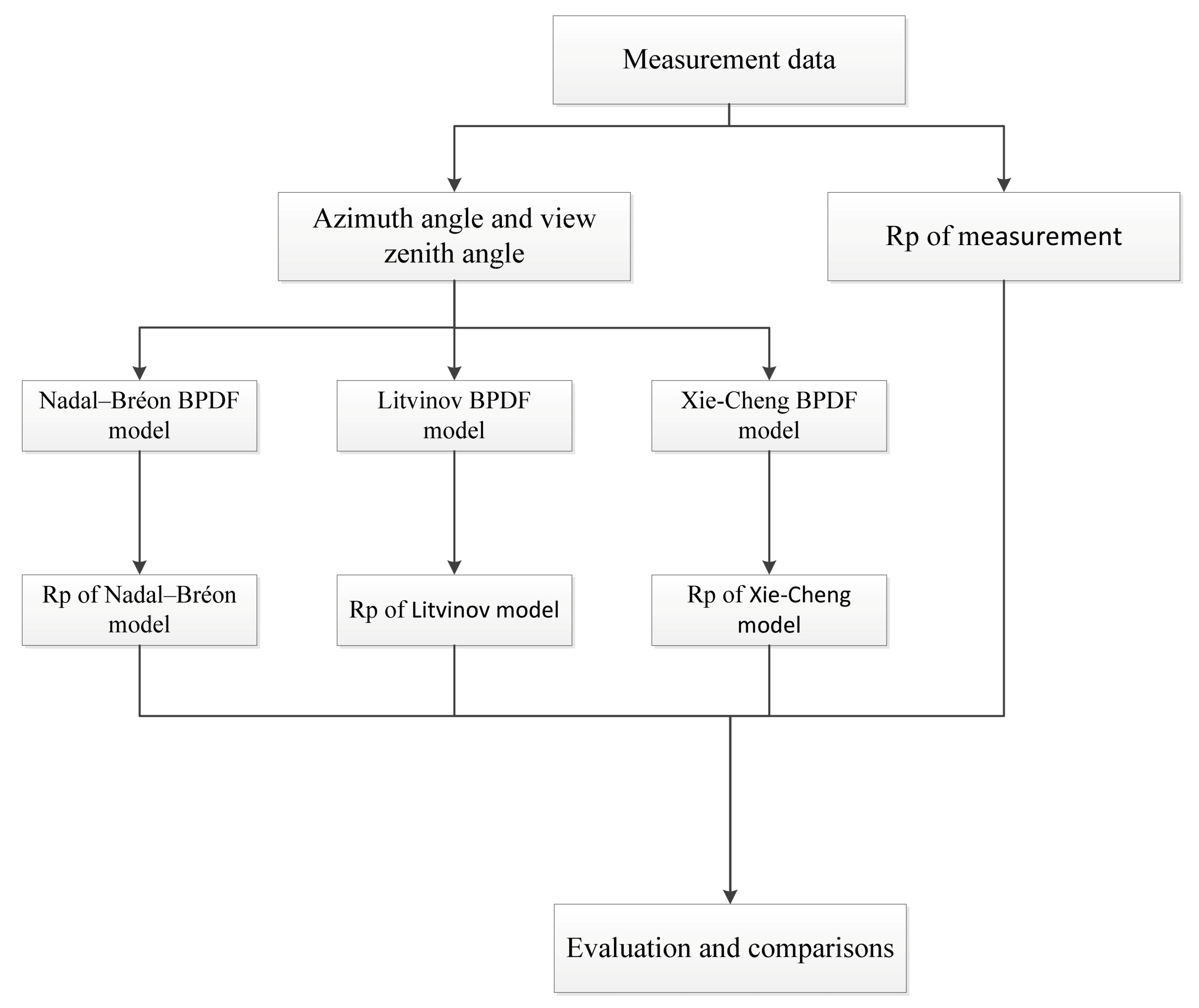The BPDF models can be broadly categorized as (a) physical models based on simplified radiative transfer equations [27,31,36] and Monte Carlo simulation [27], and (b) semi-empirical models based on the combination of physical models and free parameters that are empirically parameterized [19,22,33,37]. Six semi-empirical BPDF models were developed to parameterize the polarized reflectance of land surfaces. Using the space-borne polarization and directionality of Earth’s reflectances (POLDER) measurements, three semi-empirical BPDF models, i.e., the Nadal and Bréon model [21], the Maignan model [22], and the Xie–Cheng model [33] were proposed for 11 surface types, 14 international geosphere biosphere program (IGBP) classes, and urban areas, respectively. At the airborne level, Waquet et al. proposed a scaled Fresnel model by accounting for the mutual shadowing of facets using MICROPOL measurements over forests, cropped surfaces, and urban areas [38]. Litvinov et al. explored a three-parameter BPDF model using research scanning polarimeter (RSP) measurements over vegetation and soil surfaces [39]. For ground-level measurements, Diner et al. developed a semi-empirical BPDF model for grass surfaces using a ground-based multi-angle spectropolarimetric imager (Ground-MSPI) [37].

With the development of machine learning and deep learning methods, many algorithms have been proposed, such as the generalized regression neural network (GRNN) [40], K–nearest neighbor (KNN) algorithm [41], support vector regression (SVR) [42], random forest (RF) [43], and deep neural networks (DNN). These methods have been widely used in other fields of remote sensing, such as for classification and change detection [44,45], and in the investigation of the biophysical and biochemical characteristics of vegetation [43,46,47]. Therefore, it is possible to develop BPDF models based on machine learning using these popular algorithms. Such work, though relatively rare, is very important for improving the accuracy of inversion and enhancing the study of the polarized light characteristics of saline-alkaline soil using deep learning.

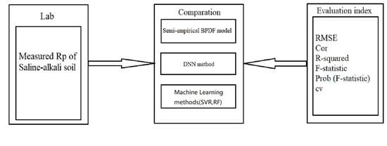
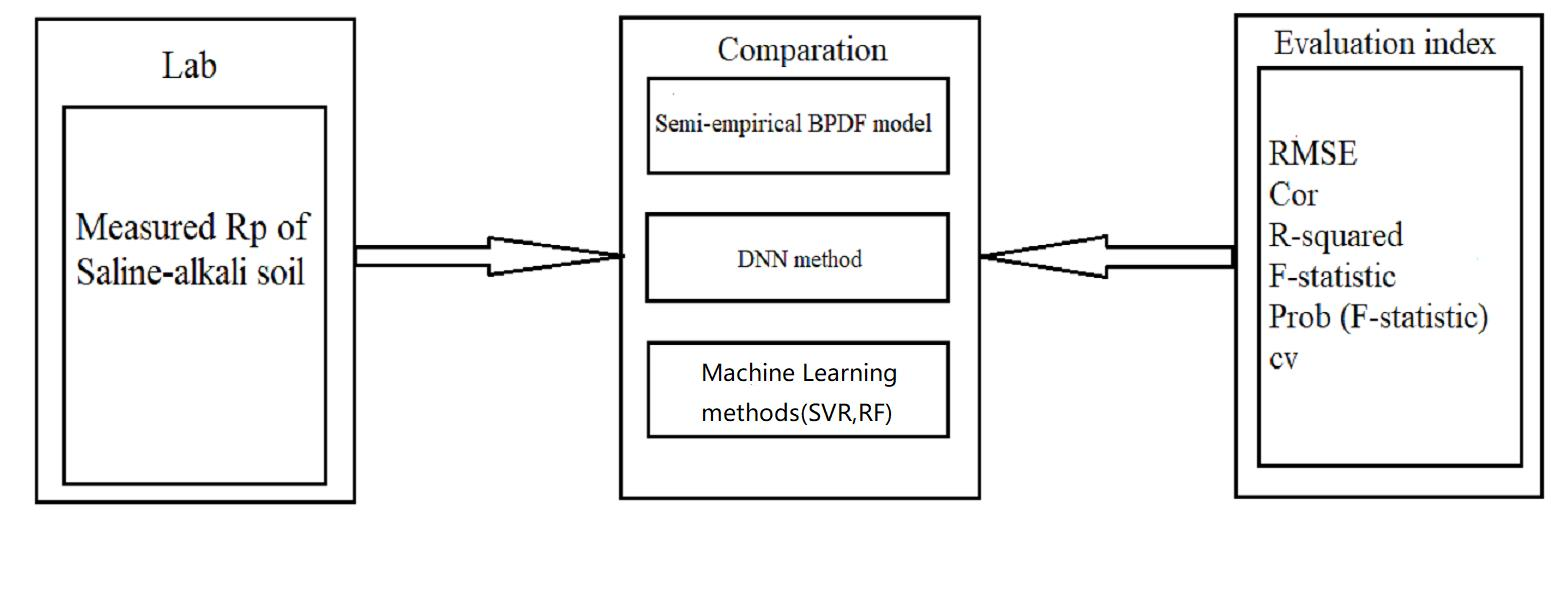
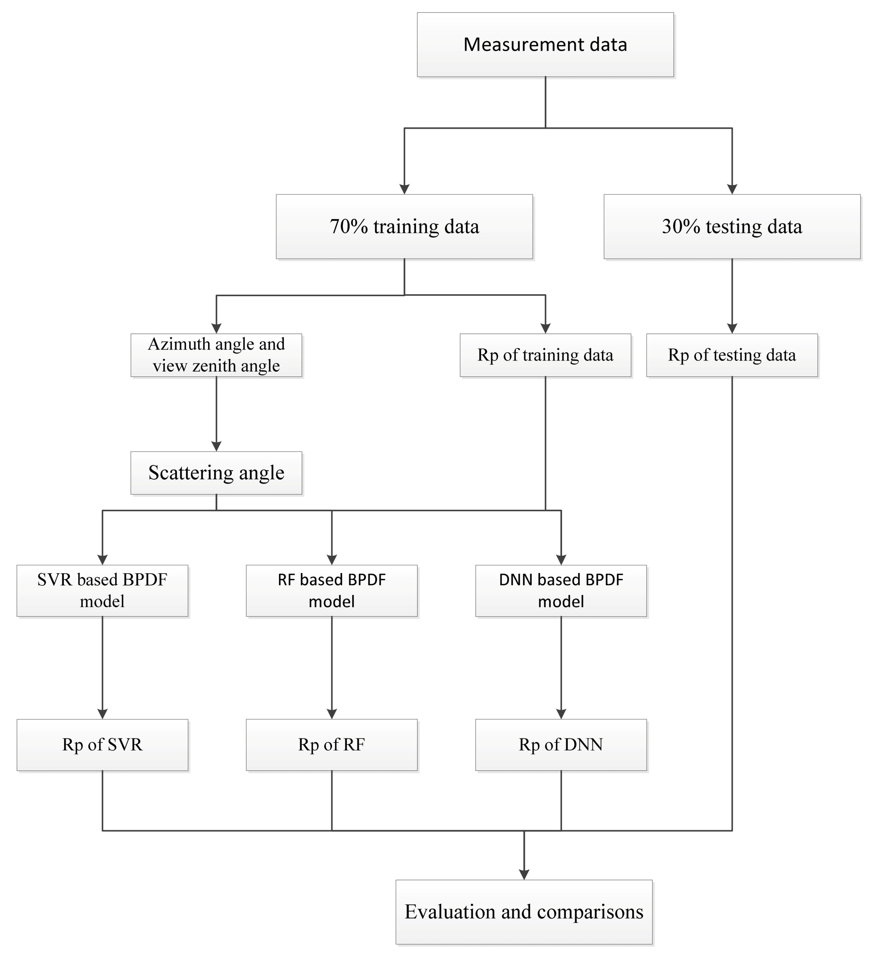
There are two main purposes of this research. The first is based on the principle of deep learning and a new method, suitable for estimating the polarization reflectivity of the saline-alkaline soil surface, is proposed. The second is to compare this new method with the existing semi-empirical BPDF model and machine learning methods, trying to establish which method is most suitable for the prediction of the polarized reflectance of a saline-alkaline soil surface. The hypothesis of this study is that the polarized reflectance of saline-alkaline soil and an ordinary soil surface is similar in some ways. The principle of deep learning can be applied for finding the solution to this problem. The method used in this research is to measure the polarized reflectance of saline-alkaline soil under laboratory conditions. After sorting the data, deep learning methods are used for processing, and the most suitable deep learning model for this research is explored by changing the corresponding parameters. In addition, using the laboratory data, the results of several existing semi-empirical BPDF models and machine learning methods are compared to achieve the purpose of this research.

2. Introduction to Models and Algorithms

Two types of models and methods for predicting the surface Rp of saline-alkaline soils were investigated in this study. One is the semi-empirical BPDF model, which mainly includes the Nadal–Bréon, Litvinov, and Xie–Cheng models. The other is a BPDF model based on machine learning, which mainly includes three methods: SVR, RF regression, and DNN. This section introduces the principles of these methods.

2.1. Semi-empirical BPDF Model

The semi-empirical BPDF model has been widely used to estimate surface Rp [48,49]. These models were originally proposed for different land cover types and were constructed based on the measurement results of different instruments [9,10,11,21,23,27,28,50]. Usually, the model data are based on POLDER measurements, and the commonly used power for surface measurement is 670 nm, 865 nm, and 1020 nm. By introducing empirically unconstrained parameters into the modeling process, it has been proven that the semi-empirical BPDF models can produce a relatively efficient calculation in the three semi-empirical models. One example is considered in this study, and the pairs generated in the three models are listed in

Table 1. Key parameter values of several semi-empirical BPDF models and BPDF models based on machine learning.

Semi-empirical BPDF Models	Nadal–Bréon model	ρ	0.025
		β	51.784
	Litvinov model	α	3.366
		σ2	0.274
		kr	0.652
	Xie–Cheng model	A	0.866
		kr	0.501
Machine Learning-based BPDF Model	SVR	γ	12.13
		C	2.58
	RF	ntree	200
	DNN	number of layers	3
		learning rate (670)	0.5
		learning rate (865)	0.4
		number of nodes	5,5,1
		activations	tanh
		optimizer	SGD

. The three models are briefly introduced below.

2.1.1. Nadal–Bréon Model

The Nadal–Bréon BPDF model is used for various natural surfaces (forests, bushes, low vegetation, and deserts). The specific models are as follows:

$${\mathrm{R}}_{\mathrm{p}}=\mathsf{\rho }\left[1-\exp \left(-\mathsf{\beta }\frac{{\mathrm{F}}_{\mathrm{p}}\left(\mathsf{\gamma }, \mathrm{N}\right)}{{\mathsf{\mu }}_{\mathrm{s}}+{\mathsf{\mu }}_{\mathrm{v}}}\right)\right]$$

(1)

$${\mathrm{F}}_{\mathrm{p}}\left(\mathsf{\gamma }, \mathrm{N}\right)=\frac{1}{2}\left[{\left(\frac{\mathrm{N}{\mathsf{\mu }}_{\mathrm{t}}-{\mathsf{\mu }}_{\mathrm{i}}}{\mathrm{N}{\mathsf{\mu }}_{\mathrm{t}}+{\mathsf{\mu }}_{\mathrm{i}}}\right)}^2-{\left(\frac{\mathrm{N}{\mathsf{\mu }}_{\mathrm{i}}-{\mathsf{\mu }}_{\mathrm{t}}}{\mathrm{N}{\mathsf{\mu }}_{\mathrm{i}}+{\mathsf{\mu }}_{\mathrm{t}}}\right)}^2\right]$$

(2)

$${\mathsf{\mu }}_{\mathrm{i}}=\cos {\mathsf{\theta }}_{\mathrm{i}},\hspace{0.17em}{\mathsf{\mu }}_{\mathrm{t}}=\cos {\mathsf{\theta }}_{\mathrm{t}}$$

(3)

$$\sin {\mathsf{\theta }}_{\mathrm{i}}=\mathrm{Nsin}{\mathsf{\theta }}_{\mathrm{t}},\hspace{0.17em}{\mathsf{\theta }}_{\mathrm{i}}=\left(\mathsf{\pi }-\mathsf{\gamma }\right)/2$$

(4)

$$\cos \mathsf{\gamma }=-\cos {\mathsf{\theta }}_{\mathrm{s}}\cos {\mathsf{\theta }}_{\mathrm{v}}-\sin {\mathsf{\theta }}_{\mathrm{s}}\sin {\mathsf{\theta }}_{\mathrm{v}}\cos \mathsf{\phi }$$

(5)

Here, $\mathsf{\rho }$ and $\mathsf{\beta }$ are the two free parameters of the model; ${\mathrm{F}}_{\mathrm{p}}\left(\mathsf{\gamma }, \mathrm{N}\right)$ indicate the Fresnel model; N is the refractive index; ${\mathsf{\theta }}_{\mathrm{i}}$ and ${\mathsf{\theta }}_{\mathrm{t}}$ are the angles of specular reflection and refraction; $\mathsf{\gamma }$ represents scattering, which is defined as the direction of the incident sun and the angle between the incident light; ${\mathsf{\mu }}_{\mathrm{s}}$ and ${\mathsf{\mu }}_{\mathrm{v}}$ represent the cosine of the solar zenith angle ${\mathsf{\theta }}_{\mathrm{s}}$ and the apparent zenith angle ${\mathsf{\theta }}_{\mathrm{v}}$, respectively; $\mathsf{\phi }$ is the relative azimuth angle between the sun and the viewing direction. It is necessary to note that the commonly accepted value of the reflective index for land surfaces is 1.5 [36].

2.1.2. Litvinov Model

The Litvinov model is a model developed by Litvinov et al., for vegetation and soil surfaces. The suppression value reflects polarized light in the forward reflection direction and introduces the shadow function with the maximum value in the backward scattering direction [32]. The specific models are as follows:

$${\mathrm{R}}_{\mathrm{p}}=\frac{{\mathsf{\alpha }\mathsf{\pi }\mathrm{F}}_{\mathrm{p}}\left(\mathsf{\gamma }, \mathrm{N}\right)}{4\cos \mathsf{\vartheta }\left({\mathsf{\mu }}_{\mathrm{s}}+{\mathsf{\mu }}_{\mathrm{v}}\right)}\mathrm{f}\left(\mathsf{\sigma },\mathsf{\vartheta }\right){\mathrm{f}}_{\mathrm{sh}}\left(\mathsf{\gamma },{\mathrm{k}}_{\mathrm{r}}\right)$$

(6)

$$\mathrm{f}\left(\mathsf{\sigma },\mathsf{\vartheta }\right)=\frac{1}{{\mathsf{\pi }\cos }^3\mathsf{\vartheta }2{\mathsf{\sigma }}^2}\exp \left(-\frac{{\tan }^2\mathsf{\vartheta }}{2{\mathsf{\sigma }}^2}\right)$$

(7)

$${\mathrm{f}}_{\mathrm{sh}}\left(\mathsf{\gamma },{\mathrm{k}}_{\mathrm{r}}\right)={\left(\frac{1+{\cos \mathrm{k}}_{\mathrm{r}}\left(\mathsf{\pi }-\mathsf{\gamma }\right)}{2}\right)}^3$$

(8)

$$\cos \mathsf{\vartheta }=\frac{{\mathsf{\mu }}_{\mathrm{s}}+{\mathsf{\mu }}_{\mathrm{v}}}{2{\mathsf{\mu }}_{\mathrm{i}}}$$

(9)

Among these, $\mathsf{\alpha }, \mathsf{\sigma },$ and ${\mathrm{k}}_{\mathrm{r}}$ are the three free parameters of the model. The function $\mathrm{f}\left(\mathsf{\sigma },\mathsf{\vartheta }\right)$ describes the Gaussian distribution of the small plane in the volume, and ${\mathrm{f}}_{\mathrm{sh}}\left(\mathsf{\gamma },{\mathrm{k}}_{\mathrm{r}}\right)$ is the shadow function with the free parameter ${\mathrm{k}}_{\mathrm{r}}$, which controls the shadow and the width of the area (0 <${ \mathrm{k}}_{\mathrm{r}}$ < 1).

2.1.3. Xie–Cheng Model

The Xie–Cheng model is proposed for urban areas, and this model can be written as:

$${\mathrm{R}}_{\mathrm{p}}=\mathrm{A}·{\mathrm{f}}_{\mathrm{sh}}\left(\mathsf{\gamma },{\mathrm{k}}_{\mathrm{r}}\right)·{\mathrm{F}}_{\mathrm{p}}\left(\mathsf{\gamma }, \mathrm{N}\right)·\exp \left(-\mathsf{\omega }, \mathrm{NDVI}\right)$$

(10)

$$\mathrm{NDVI}=\frac{\mathrm{NIR}-\mathrm{R}}{\mathrm{NIR}+\mathrm{R}}$$

(11)

Here, A and ${\mathrm{k}}_{\mathrm{r}}$ are the two free parameters of the model. $\mathsf{\omega }$ is an experimental parameter that compensates for the influence of NDVI on polarized reflectance. and it is recommended to be equal to 0.7 [33]. NDVI means the normalized difference vegetation index. This is one of the most important parameters reflecting crop growth and nutritional information. NIR is the reflection value of the near-infrared band, and R is the reflection value of the red-light band [51].

The prediction process for Rp on the surface of a saline-alkaline soil using the semi-empirical BPDF model is as follows:

• Step 1: input the azimuth, detection angle, and model parameters from the experiment to the semi-empirical BPDF model and calculate the predicted Rp.
• Step 2: compare and fit the measured Rp in the laboratory with the predicted Rp and use the root mean squared error (RMSE), correlation coefficient (Cor) and R-squared (R²) to evaluate the results.

The specific process is shown in Figure 1.

2.2. BPDF Model Based on Machine Learning

Three machine learning regression algorithms, SVR, RF, and DNN, were used in this study to establish a machine learning-based BPDF model. All four algorithms were implemented using Python. The schematic diagram of the DNN model is shown in Figure 2. A brief flow of the three machine learning algorithms is shown in Figure 3, and the parameters involved are listed in Table 1.

2.2.1. Support Vector Regression (SVR)

SVR is a regression implementation of a support vector machine (SVM). Based on the SVR algorithm among various types, this study uses the classical and widely used $\mathsf{\epsilon }$-SVR [40,41,42]. $\mathsf{\epsilon }$-SVR uses a kernel function to convert the input data into a high-dimensional feature space, and then uses a support vector whose training error lies beyond the $\mathsf{\epsilon }$ edge to establish the super parameters of the regression function. A nonlinear Gaussian RBF was used in this study, and the parameter γ was adjusted as the kernel function. γ controls the basic radius of the RBF, which reflects the size of each support vector of the sensitive area. A larger γ indicates that the sensitive area of the RBF is narrower, i.e., the model is more likely to be overfitted. In the loss function, the regularization constant C is used to control the trade-offs on the support vector, while the observations in the ε tube are not penalized. A larger C will also lead to a greater possibility of overfitting. In this study, ε was set to 0.01, and the appropriate settings of γ and C were critical to the performance of the model.

The optimization ranges of the γ and C parameters are 10⁻⁵ to 10² and 10⁻² to 10², respectively, which is similar to the configuration used in [48,49]. Furthermore, through the minimized-merit function:

$$\mathrm{RMSECV}\left({\mathsf{\gamma }}_{\mathrm{k}},{\mathrm{C}}_{\mathrm{k}}\right)=\frac{{\sum }_{\mathrm{i}=1}^{\mathrm{m}}{\mathrm{RMSE}}_{\mathrm{ith}}\left({\mathsf{\gamma }}_{\mathrm{k}},{\mathrm{C}}_{\mathrm{k}}\right)}{\mathrm{m}}$$

(12)

$\mathrm{RMSECV}\left({\mathsf{\gamma }}_{\mathrm{k}},{\mathrm{C}}_{\mathrm{k}}\right)$ is the combination of the RMSE γ and C of the k-th cross-validation used, m is the multiple of the cross-validation, ${\mathrm{RMSE}}_{\mathrm{ith}}$ is the model in the i-th iteration of the root-mean-square cross-validation estimated error.

2.2.2. Random Forest Regression

RF regression is a type of non-parameter ensemble learning algorithm [32]. RF regression grows many simultaneous decision trees and performs estimations based on the results of all trees; hence, it usually provides an effective and accurate performance [50]. In the training procedure, RF regression uses a bootstrapping approach to randomly select approximately two-thirds of the samples from the training dataset, while the remaining one-third is used to calculate the out-of-bag (OOB) error to represent the performance of the built model. To grow each tree independently, RF randomly selects one-third of the samples (two variables of the total four in this study) each time to grow each individual tree. Using the standard classification and regression tree (CART), the best splitting variable and the best splitting value are determined by minimizing the weighted impurity, G, from the left and right nodes after splitting:

$$\mathrm{G}\left({\mathrm{x}}_{\mathrm{i}},{\mathrm{v}}_{\mathrm{ij}}\right)=\frac{{\mathrm{n}}_{\mathrm{l}}}{{\mathrm{N}}_{\mathrm{t}}}\mathrm{H}\left({\mathrm{X}}_{\mathrm{l}}\right)+\frac{{\mathrm{n}}_{\mathrm{r}}}{{\mathrm{N}}_{\mathrm{t}}}\mathrm{H}\left({\mathrm{X}}_{\mathrm{r}}\right)$$

(13)

where ${\mathrm{v}}_{\mathrm{ij}}$, the splitting point, is the j-th value of the splitting variable ${\mathrm{x}}_{\mathrm{i}}$; ${\mathrm{n}}_{\mathrm{l}}$ and ${\mathrm{n}}_{\mathrm{r}}$ are the number of training samples of the left and right nodes after splitting, respectively; ${\mathrm{N}}_{\mathrm{t}}$ is the number of training samples of the node to be split; and $\mathrm{H}\left({\mathrm{X}}_{\mathrm{l}}\right)$ or $\mathrm{H}\left({\mathrm{X}}_{\mathrm{r}}\right)$ is the impurity function of the left or right node. For the regression problem, the mean squared error (MSE) serves as the $\mathrm{H}\left(\mathrm{X}\right)$. MSE is defined as the mean square of the deviation between the training targets and their average within a node after splitting. In the prediction procedure, the average of the predictions of all trees is taken as the estimated output value for each query input observation.

The two key parameters of RF regression, the number of trees (ntree) and the smallest terminal node leaf (node size), have a significant impact on model performance. The smaller the ntree node, the larger the size, the denser the forest, and the deeper the trees. In this study, the node size was set to 5, to balance the training accuracy and generalization ability of the model [43]. The ntree was set at 200 for a better outcome, as it has been established that a value greater than 100 ntree can ensure the stability of the RF model [48,49]. The RF regression was implemented using the Sklearn package in Python.

2.2.3. Deep Neural Network Regression

After years of development, deep learning has derived a variety of different structures to solve various problems [52] and has gradually achieved better results in various application scenarios. A neural network is the basic unit of all deep learning models and is usually used to estimate complex functional relationships that are difficult to express directly. A neural network consists of an input layer, zero or more hidden layers, and an output layer. Figure 2 shows a neural network with two hidden layers. The process of transferring data from the input layer to the output layer is called forward propagation. The data transmission between two adjacent layers can be expressed as:

$${\mathrm{a}}_{\mathrm{i}}=\mathrm{f}\left({\mathrm{W}}_{\mathrm{i}}{\mathrm{a}}_{\mathrm{i}-1}+{\mathrm{b}}_{\mathrm{i}}\right)$$

(14)

where ${\mathrm{a}}_{\mathrm{i}-1}$ and ${\mathrm{a}}_{\mathrm{i}}$ represent the output of the (i-1)-th layer and the i-th layer, respectively; ${\mathrm{W}}_{\mathrm{i}}$ and ${\mathrm{b}}_{\mathrm{i}}$ represent the weight matrix parameter and offset vector parameter, respectively; and $\mathrm{f}$ represents the activation function. The connection between adjacent neurons in Figure 2 represents a certain parameter in the weight matrix, except that each neuron in the input layer has an offset parameter. The activation function causes the neuron to have a nonlinear output. Commonly used activation functions include sigmoid, tanh, and Relu. A schematic of the DNN is shown in Figure 2.

Normally, the number of neurons in the input and output layers is relatively easy to determine, according to the problem. The key is to select the appropriate number of hidden layers and the number of neurons in each hidden layer. The more parameters of the neural network, the stronger its performance; however, it is then prone to overfitting. In addition, the loss function used to measure the difference between the output of the neural network and the target value needs to be selected according to the scene. The MSE and cross-entropy loss are frequently used as loss functions. The purpose of the training was to minimize the loss function. First, the backpropagation algorithm is used to find the derivative of the loss function for each parameter, and then methods such as stochastic gradient descent are used to update the parameters.

The deep learning method used in this research is CNN (deep convolutional neural networks). This is a commonly used deep learning algorithm that has a wide range of applications in image recognition, image segmentation, speech recognition, and other fields. It has achieved better results in the above areas [53]. In addition, CNN can also be used for regression prediction and other aspects. This study tried to use this method to deal with the problem of the polarization reflectivity of saline-alkaline soil. The BPDF model, based on machine learning, was used to predict the surface Rp of saline-alkaline soil, as detailed below. A schematic of the process is shown in Figure 3.

• Step 1: input the azimuth angle, detection angle, and solar zenith angle from the experiment into the formula to calculate the scattering angle, as one of the input variables. The Rp of the saline-alkaline soil surface measured in the laboratory was used as another input variable.
• Step 2: take 70% of the laboratory data as the experimental group to train the neural network.
• Step 3: use the remaining 30% of the laboratory data as the test group, to verify the effect of the network trained by deep learning.

The specific parameters and methods of several machine learning methods used in this research are listed in Table 1. A detailed explanation of tuning the learning rate parameter is included in Section 5.2.

2.3. Definition of the Evaluation Index

This study uses various indicators to judge the performance of the model. The corresponding definition is given below.

2.3.1. Root Mean Square Error (RMSE)

The RMSE is the deviation between the measured value and the true value. It is often used as a standard for measuring the prediction results of machine learning models [54].

$$\mathrm{RMSE}=\sqrt{\frac{1}{\mathrm{m}}{\displaystyle \sum }_{\mathrm{i}=1}^{\mathrm{m}}{\left({\mathrm{y}}_{\mathrm{i}}-\widehat{{\mathrm{y}}_{\mathrm{i}}}\right)}^2}$$

(15)

where ${\mathrm{y}}_{\mathrm{i}}$ refers to the true value of the sample, and $\widehat{{\mathrm{y}}_{\mathrm{i}}}$ refers to the predicted value. The m symbol refers to the number of samples. RMSE is an index greater than zero, and the closer its value is to 0, the better the model effect.

2.3.2. R-Squared (R²)

R² is an important statistic reflecting the goodness of the model fit. It uses the mean model as the baseline model, to facilitate the comparison of the models corresponding to different dimension data sets [55]:

$${\mathrm{R}}^2=1-\frac{{\sum }_{\mathrm{i}=1}^{\mathrm{m}}{\left({\hat{\mathrm{y}}}_{\mathrm{i}}-{\mathrm{y}}_{\mathrm{i}}\right)}^2}{{\sum }_{\mathrm{i}=1}^{\mathrm{m}}{\left(\overline{\mathrm{y}}-{\mathrm{y}}_{\mathrm{i}}\right)}^2}$$

(16)

where $y_i$ refers to the true value of the sample, and $\widehat{y_i}$ refers to the predicted value. The symbol $\overline{y}$ refers to the mean of the sample. The m symbol refers to the number of samples. The value of R² is between 0 and 1. The closer its value is to 1, the better the model effect.

2.3.3. Correlation Coefficient (Cor)

The correlation coefficient is used to measure the correlation between two variables [56]:

$$\mathrm{Cor}\left(\mathrm{X},\mathrm{Y}\right)=\frac{\mathrm{Cor}\left(\mathrm{X},\mathrm{Y}\right)}{\sqrt{\mathrm{Var}\left(\mathrm{X}\mathrm{\right)}\mathrm{Var}\left(\mathrm{Y}\right)}}$$

(17)

where Cov (X, Y) is the covariance of X and Y, Var(X) is the variance of X, and Var(Y) is the variance of Y. The value of Cor is between −1 and 1. The closer its value is to 1 or −1, the stronger the relationship between X and Y.

2.3.4. F-Statistic

An F-statistic is a value you get when you run an ANOVA test or a regression analysis to find out if the means between two populations are significantly different. It is similar to a T statistic from a t-Test; a t-test will tell you if a single variable is statistically significant, and an F-test will tell you if a group of variables is jointly significant:

$$\mathrm{F}=\frac{{\mathrm{S}}_{\mathrm{x}}^2}{{\mathrm{S}}_{\mathrm{y}}^2}$$

(18)

where ${\mathrm{S}}_{\mathrm{x}}^2$ and ${\mathrm{S}}_{\mathrm{y}}^2$ are variance of X and Y. The F value in regression is the result of a test where the null hypothesis is that all the regression coefficients are equal to zero. In other words, the model has no predictive capability. Basically, the F-test compares your model with zero predictor variables (the intercept-only model) and decides whether your added coefficients improved the model. If you get a significant result, then whatever coefficients you included in your model improved the model’s fit. In other words, the larger the value of the F-statistic, the better the significance. The smaller the value, the significance is worse.

Before comparing F-values, you need to pay attention to Prob (F-statistic). If the Prob (F-statistic) is small (for example, less than 0.01, depending on your alpha level), you can reject the null hypothesis. Only then should you consider the F-value. If you do not reject the null hypothesis, ignore the f-value [57].

2.3.5. Coefficient of Variation (cv)

The coefficient of variation is also known as the coefficient of dispersion. It is a non-dimensional statistic that measures the degree of data dispersion [58]:

$$\mathrm{CV}=\frac{\mathsf{\sigma }}{\mathsf{\mu }}$$

(19)

where $\mathsf{\sigma }$ is a standard deviation of the data and $\mathsf{\mu }$ is the mean of the data. Compared with the standard deviation, the coefficient variation can better compare the degree of dispersion of several sets of data with different dimensions and different scales.

3. Data Description

3.1. Study Area

The soil samples used in this experiment were obtained from Zhenlai County, Baicheng City, Jilin Province, China, at 122°47′ E–124°04′ E, 45°28′ N–46°18′ N). The area belongs to the western Songnen Plain, which is in the northeast of China and northwest of Heilongjiang Province. The relative positional relationships are shown in Figure 4. The climate has a typical semi-arid monsoon climate. Precipitation decreases from the east (420–460 mm) to the west (350–420 mm), and evaporation increases from the east (1200–1600 mm) to the west (1500–1900 mm) [59,60]. Due to the high groundwater level, high salinity, high evaporation rate, and insufficient drainage, soil salinization in the Songnen Plain is a very serious problem. The Songnen Plain is one of the main saline-alkaline soil areas in China, and it is one of the three major accumulation areas of soda saline soil worldwide [61]. The main components of soda saline soil are Na₂CO₃, NaHCO₃, and NaCl in the Songnen Plain [62]. These types of soda saline soil are very stable in the top 20-cm of the soil layer and, to a large extent, prevent the salt from moving downward due to poor permeability [63]. In addition, since the Songnen plain is one of the main food production centers, the most serious cause of secondary salinity is frequently human activities [64].

3.2. Soil Sample Processing

Using the following method, 50 topsoil samples (depth < 10 cm) were collected for stratified sampling in October 2020, and their GPS locations were recorded. The collected soil samples were moved to the laboratory, and the soil collected from the field was first dried, then ground, and finally sieved through a 100-mesh sieve with a 0.15-mm aperture. The grinding and screening process was repeated until the soil particles were sufficiently small. Subsequently, NaHCO₃ and NaCl were added to the sample to configure the saline-alkaline soil with different electrical conductivity (EC) and salinity levels. Several key parameters of the soil used in this research experiment are listed in

Table 2. Key parameters of experimental soil.

	Minimum	Maximum
EC (ds/m)	0.930	5.510
pH	8.190	9.490
C (%)	1.210	2.130
N (%)	0.014	0.078

. The ratio of the sample to the solution used for the measurement of the EC and pH values was 1:1.

3.3. Spectral Measurement Process

This subsection describes the process of measuring surface polarization reflectivity. The field of view was 8°, the distance from the sensor to the sample was 0.2 m, and the zenith angle of the sensor changed from 0° to 60°. For the laboratory measurement, we placed the samples on the stage such that they were close to the standardized measurement plane, and the illuminated center line intersected the viewing direction. The polarization angles of the polarization lens were 0°, 45°, 90°, and 135°, and the final polarization reflectivity was the average of the four polarization angles. When measuring the sample, it was placed on a black background with a reflectivity of 5%. The edge of the sample was parallel to the main plane in the wavelength range of 400–1000 nm. During the experiment, the zenith angle of illumination was maintained at 40°. First, we fixed an azimuth angle and changed to different zenith angles to observe the sample. The zenith angle started at 10°, and changes to 60°at intervals of 10° (10°, 20°, 30°, 40°, 50°, 60°). After that, we changed the azimuth at 20° intervals, fixed an azimuth, and repeated the previous steps until it changed from 0° to 180°. In addition, we replaced the values of the 0° azimuth and 40° detection angle with a 0° azimuth and 32° detection angle. All measurements were based on the assumption that the reflectance was symmetrical, and the polarized sample surface relative to the main plane source has been verified by Maignan et al. [22]. The schematic diagram of the experimental process is shown in Figure 5.

4. Results

4.1. Spectral Measurement Results

Figure 6 shows the variation of saline-alkaline soil Rp with its wavelength under different azimuth angles and different detection angles. Different colors indicate different detection angles and azimuths. Figure 6a shows the polarization reflectivity of different detection angles varying with the wavelength when the azimuth angle is 0°. Clearly, at the wavelength range of 400–1000 nm, when the azimuth angle is 0°, the polarization reflectivity is the largest when the detection angle is 60° and the smallest when the detection angle is 0°. When the detection angle was increased from 0° to 60°, Rp gradually increased. As shown in Figure 6b, when the observation angle was 20°, the polarization reflectivity at different azimuth angles varied with the wavelength. Furthermore, at the wavelength range of 400–1000 nm and detection angle of 20°, the polarization reflectivity was the largest when the azimuth angle was 0°, and the polarization reflectivity was the smallest when the azimuth angle was 180°. In addition, when the detection angle was increased from 0° to 180°, Rp decreased sequentially.

Four absorption features were used for judgment, near 1000 nm, 1400 nm, 1900 nm, and 2200 nm. This feature is obvious, whether it is at a fixed azimuth angle or detection angle. At the same time, some other slight absorption features were observed near 1100, 1800, and 2400 nm. As discussed in the literature, crystal lattices of hydrated minerals formed of internal hydroxide ions and water were observed at 1000 nm, 1100 nm, and 1800 nm [65,66]. The deeper absorption near 1400 nm and 1900 nm may be the result of O–H stretching and H–O–H bending, and the basic sand overtone [67]. Anhydrous evaporating minerals containing ${\mathrm{CO}}_3^{2-}$ and ${\mathrm{HCO}}_3^{-} ,$ due to the vibration of the carbonate group (for example, the wavelengths near 1800 nm, 1900 nm, 2200 nm, and 2300 nm), exceed 1600 nm, and there are many spectral features at the wavelength [65,67].

Owing to the measurement principle of the ground object spectrometer (Analytical Spectral Devices FieldSpec3 spectrometer (ASD FS3, Boulder, CO, USA)), there was splicing of the spectrum at 1000 nm and 1800 nm which led to the oscillation of the spectral line after 1000 nm, as seen in Figure 6a. However, the measurement results in the range of 400–1000 nm were good, the polarization reflectance line graph did not appear to cross, and the result was obvious. As mentioned in the previous document [35], the data used in the semi-empirical BPDF model are POLDER measurement data. As this study focuses on the measurement of surface reflectance, the two bands of 670 nm and 865 nm are used for follow-up work.

4.2. Semi-Empirical BPDF Model Results

Figure 7 shows the fit of the saline-alkaline soil surface Rp, as predicted by the semi-empirical BPDF model and the actual measured Rp. For each scatter plot, the corresponding RMSE, Cor, and R² were calculated to characterize the effects of the fitting and facilitate subsequent comparisons. The results are as follows: (a) 670 nm Nadal–Bréon model, (b) 865 nm Nadal–Bréon model, (c) 670 nm Litvinov model, (d) 865 nm Litvinov model, (e) 670 nm Xie–Cheng model, and (f) 865 nm Xie–Cheng model.

4.3. Machine Learning Methods Prediction Results

Figure 8 shows a scatter plot, based on the machine learning BPDF model, to predict the surface Rp of the saline-alkaline soil and the actual measured value. For each scatter plot, the corresponding RMSE, Cor, and R² were calculated to facilitate future comparisons. The results are as follows: (a) 670 nm SVR, (b) 865 nm SVR, (c) 670 nm RF, (d) 865 nm RF, (e) 670 nm DNN, and (f) 865 nm DNN.

4.4. Comparison and Analysis of Semi-Empirical BPDF and BPDF Models Based on Machine Learning

Table 3. Fitting results of three semi-empirical BPDF models and three BPDF models, based on machine learning, using RMSE and Cor parameters to show the fitting effect.

Band	Index	Semi-empirical BPDF Models			Machine Learning
		Nadal–Bréon	Litvinov Model	Xie–Cheng Model	SVR	RF	DNN
670 nm	RMSE	0.0372	0.0359	0.0361	0.0425	0.0384	0.0348
	Cor	0.8935	0.8884	0.8625	0.9275	0.8785	0.9316
	R2	0.6572	0.6700	0.6452	0.4651	0.6994	0.7521
865 nm	RMSE	0.0613	0.0579	0.0562	0.0492	0.0476	0.0451
	Cor	0.9335	0.9336	0.9055	0.8791	0.8973	0.8917
	R2	0.4376	0.4995	0.5127	0.6059	0.7426	0.7692

compares the fitting effects of the semi-empirical BPDF model and BPDF model, based on machine learning. First, we compared the RMSE of the fitting results. In the 670 nm band, the minimum value of the semi-empirical BPDF model was achieved by the Litvinov model, and the minimum value in the processing results of the machine learning method was obtained using the DNN method. In comparison, the RMSE predicted by the DNN method was 3.06% lower than that of the Litvinov model. In the case of the 865 nm band, the minimum value of the semi-empirical BPDF model was achieved by the Xie–Cheng model, and the minimum value of the processing results of the BPDF model method, based on machine learning, was obtained by the DNN method. In comparison, the RMSE of the predicted result of the DNN method was 19.75% lower than that of the Xie–Cheng model. In addition to DNN, the other two methods, SVR and RF, have different degrees of improvement compared to the results of the semi-empirical BPDF model in most cases. Therefore, the RMSE value of the fitting result of the BPDF model based on machine learning was smaller, and the fitting result was more concentrated.

Next, we compared the Cor of different bands. Clearly, fitting correlation coefficients between the prediction results of the semi-empirical BPDF model or the machine learning method and the laboratory measurement results were all greater than 0.8, indicating that the fitting effects of several methods were relatively good. In addition, the Cor value of the processing result of the machine learning in the 670 nm band was greater than that of the semi-empirical BPDF model, except for the RF method. Among them, the maximum value of the semi-empirical BPDF model was achieved by the Nadal–Bréon model, and the maximum value in the processing results of the machine learning method was obtained using the DNN method. In comparison, the Cor predicted by the DNN method was 4.26% higher than that predicted by the Nadal–Bréon model. In the case of the 865 nm band, the maximum value of the semi-empirical BPDF model was achieved by the Litvinov model, and the maximum value in the processing results of the machine learning method was obtained by the RF method. Although the Cor value of the machine learning method fitting results was less than that obtained by the BPDF model fitting, the difference between the two was small, and the Cor value was very close to 0.9. Clearly, the fitting results of the machine learning method were also relatively good. This situation occurred in the 865 nm band because the machine learning method divides the dataset into two parts: the training group and the control group. However, different grouping ratios also affect the final fitting results, which will be discussed later. The influence of the grouping ratio on the fitting results was discussed in detail.

In addition, we compared the R² of different bands. Regardless of whether it is 670 nm or 865 nm, the R² value predicted by the machine learning method is higher than the R² value predicted by the semi-empirical model. Among them, in the semi-empirical model, the best results in the 670 nm band were obtained from the Litvinov model. In the 865 nm band, the best results are obtained with the Xie–Cheng model. The best results in the 670 nm band and the 865 nm band in the machine learning method were obtained by the DNN method. The result of RF was also better, which is closer to the DNN method.

Lastly, we also introduced relevant indicators to evaluate the variability and statistical significance of the results. In

Table 4. The variability and statistical significance of the semi-empirical BPDF models and machine learning methods. Here, F-statistic and Prob (F-statistic) are used to characterize the significance of the results. The cv are used to characterize the variability of the results.

Index	Semi-Empirical BPDF Models						Machine Learning
	Nadal–Bréon		Litvinov Model		Xie–Cheng Model		SVR		RF		DNN
	670 nm	865 nm	670 nm	865 nm	670 nm	865 nm	670 nm	865 nm	670 nm	865 nm	670 nm	865 nm
F-statistic	1518	1934	1500	2052	1253	1560	175.7	185.5	272.3	296.5	612.9	353.4
Prob (F-statistic)	4.61 × 10−51	3.04 × 10−46	3.84 × 10−53	2.42 × 10−50	4.88 × 10−51	3.91 × 10−48	5.74 × 10−12	1.41 × 10−11	1.80 × 10−16	1.84 × 10−13	1.48 × 10−17	3.51 × 10−14
cv	0.5333	0.5171	0.5505	0.5301	0.5361	0.5216	0.1518	0.2616	0.5281	0.4784	0.5184	0.5246

, F-statistic and Prob (F-statistic) are used to characterize the significance of the results. The cv is used to characterize the variability of the results. The Prob (F-statistic) of all models are less than 0.01, and the F-statistic value is relatively large, so there is a greater probability of rejecting the null hypothesis, that is, the significance of the semi-empirical BPDF model and the regression results of the machine learning method is relatively good. In addition, the significance of semi-empirical BPDF models is better than machine learning methods. The best semi-empirical BPDF model is the Litvinov model, and the best machine learning method is the DNN method. The cv of all model results are relatively similar, around 0.5, except for the SVR results.

5. Discussion

The discussion is divided into three parts. The first and second parts discuss the parameters of the machine learning methods and try to find the best method. Compared with the BPDF model based on machine learning, the semi-empirical BPDF model is more advanced, owing to years of research. However, there are few results regarding the BPDF model based on machine learning. In addition, according to the principles of machine learning, many factors affect the final results of machine learning, for example, data quality, the ratio of the training set and test set, learning rate, etc. These factors largely depend on past experience. The DNN-BPDF model has limited reference research available, so this section will further discuss the training set size and learning rate.

5.1. Influence of the Training Ratio on the Fitting Effect

According to the principles of machine learning, the original dataset needs to be divided into two parts: a training set and a test set. The training set is used to train the model so that the model fits the problem to be studied. The test set is used to evaluate the fitness of the model [52]. The training set has an impact on the training results. If extremely little data is used for training, then the model is not fully trained, and it is difficult to achieve the desired effect; if an excessive amount of data is used for training, the test set will be too small. The fitting situation will also affect the final result in an unsatisfactory manner. In addition, the choice of training ratio will vary depending on the research problem, and the method of choosing the best training ratio is based on experience. Therefore, it is necessary for us to discuss the training ratios.

To illustrate the impact of the training and test data ratio on the final result, we selected the training data ratios as 10%, 20%, 30%, 40%, 50%, 60%, 70%, and 80% at 670 nm. The RMSE, Cor, and R² values, based on the degree of fit of the machine learning BPDF model in several cases, are calculated at the two bands of 865 nm. The results are shown in

Table 5. Fitting results of different training ratios in the 670 nm band. The best results of each index are expressed in bold font.

670 nm	Machine Learning
	SVR			RF			DNN
Training Ratio (%)	RMSE	Cor	R2	RMSE	Cor	R2	RMSE	Cor	R2
10	0.0713	0.4357	0.0542	0.0552	0.6421	0.2043	0.0628	0.5123	0.045
20	0.0751	0.3653	0.1436	0.0622	0.5395	0.1008	0.0828	0.0103	0.086
30	0.0674	0.2965	0.2013	0.0445	0.7632	0.4834	0.0418	0.8231	0.6084
40	0.0703	0.4376	0.1963	0.0553	0.7038	0.3547	0.0456	0.8421	0.5455
50	0.0683	0.8632	0.2675	0.0506	0.7558	0.4896	0.0436	0.8319	0.6201
60	0.0534	0.8953	0.2141	0.0451	0.7691	0.5621	0.0339	0.8911	0.7471
70	0.0425	0.9275	0.4651	0.0384	0.8785	0.6994	0.0348	0.9316	0.7521
80	0.0458	0.9348	0.4765	0.0437	0.8566	0.6101	0.0379	0.9339	0.7068

and

Table 6. Fitting results of different training ratios in the 865 nm band. The best results of each index are expressed in bold font.

865 nm	Machine Learning
	SVR			RF			DNN
Training Ratio (%)	RMSE	Cor	R2	RMSE	Cor	R2	RMSE	Cor	R2
10	0.0717	0.8892	0.2015	0.0586	0.7255	0.4662	0.0762	0.8026	0.1001
20	0.0745	0.8951	0.2011	0.0454	0.8495	0.7034	0.0438	0.8621	0.7232
30	0.0743	0.8901	0.1963	0.0396	0.8831	0.7717	0.0368	0.9002	0.7981
40	0.0515	0.8743	0.6028	0.0393	0.8701	0.7757	0.0352	0.9077	0.8193
50	0.0517	0.8924	0.6197	0.0471	0.8684	0.6841	0.0383	0.9038	0.7913
60	0.0551	0.8871	0.6119	0.0443	0.9085	0.7489	0.0412	0.9011	0.7833
70	0.0492	0.8791	0.6059	0.0476	0.8973	0.7426	0.0451	0.8917	0.7692
80	0.0572	0.9087	0.6211	0.0612	0.8761	0.5667	0.0541	0.9276	0.6618

. However, when the proportion of the training set is particularly small, the training results may be unsatisfactory, due to the small number of samples. This study uses oversampling to alleviate the problem of insufficient samples [68]. The results shown in Table 5 and Table 6 are the results of this method.

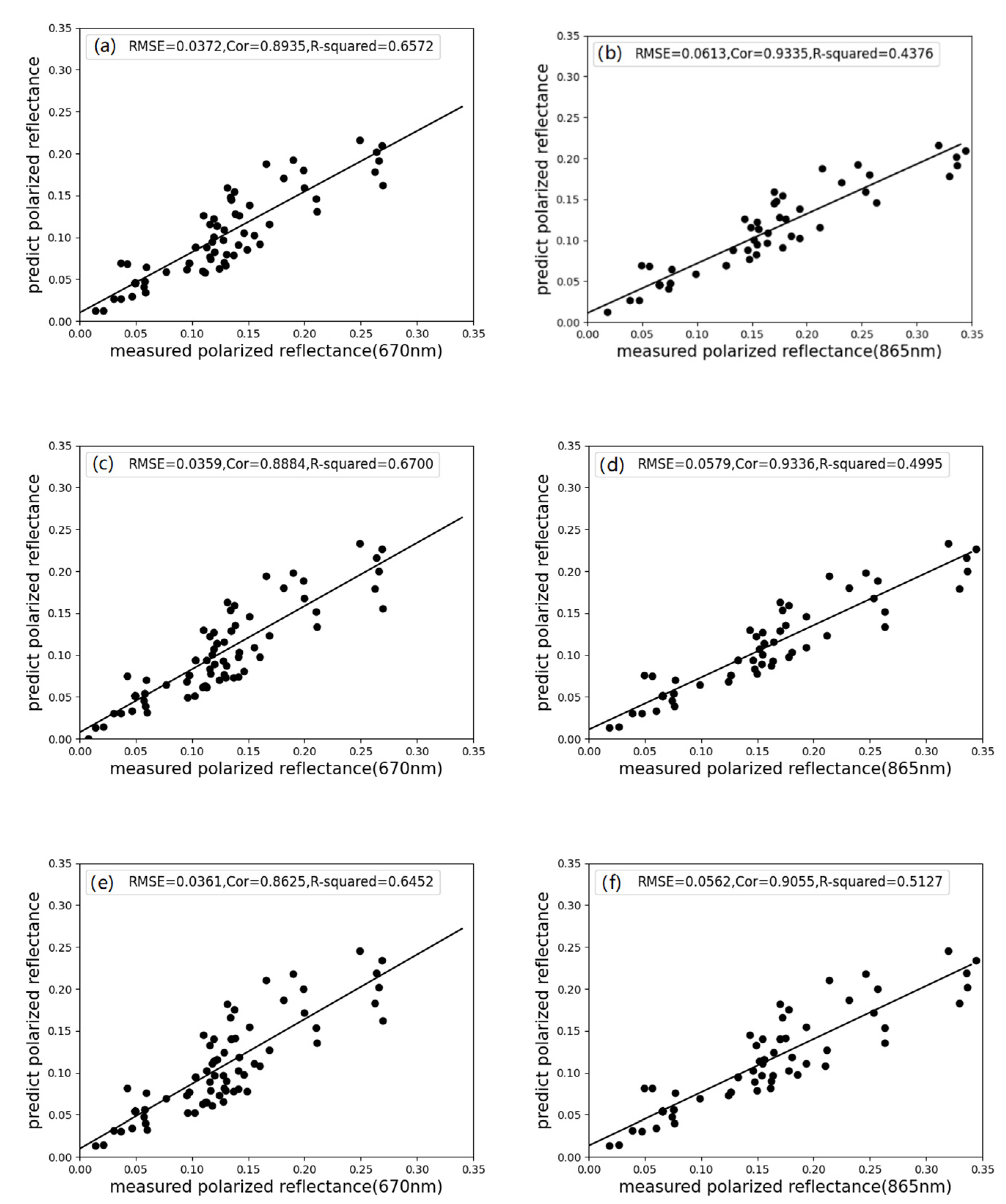
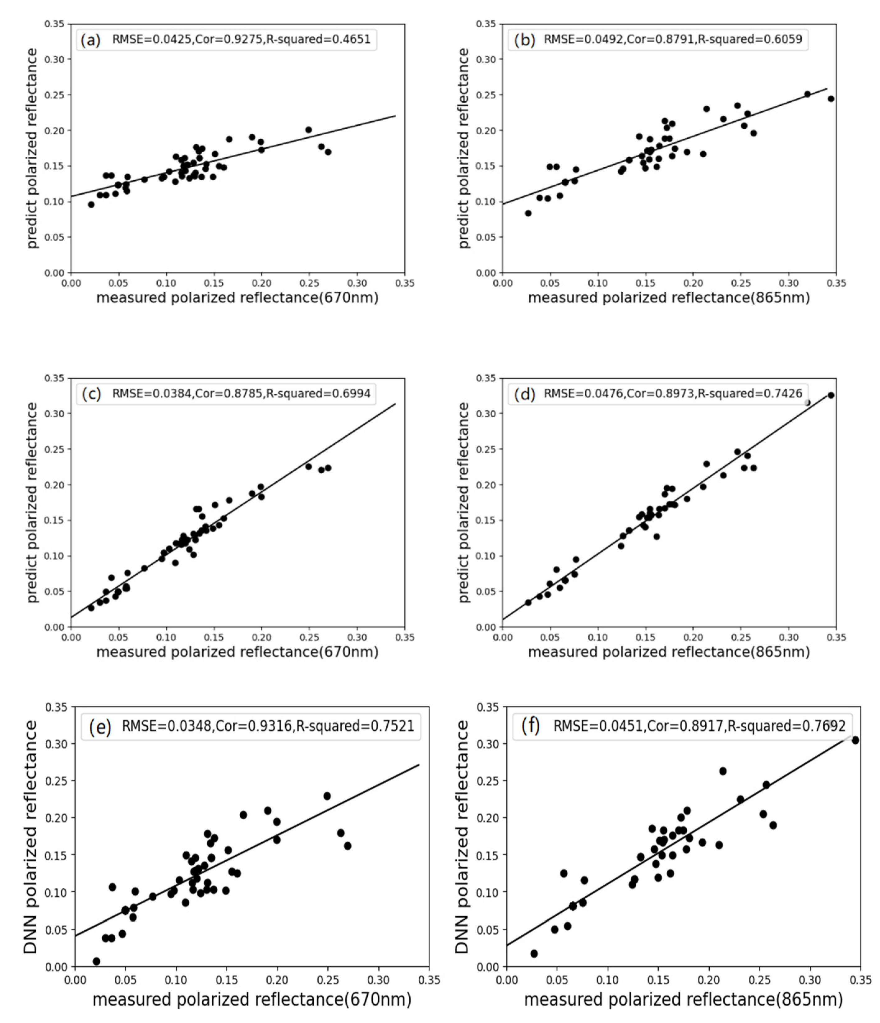
The above two tables show the influence of different grouping ratios on the fitting effect. The numbers in bold type indicate the best effect among the statistics. It is clear that the optimal results in the 670 nm band are concentrated in the 60–80% proportion of the training set, and the optimal results in the 865 nm band are concentrated in the 50–80% proportion of the training set. Therefore, the grouping ratio adopted in this experiment, that is, the 70% training set and 30% test set, has a relatively good fitting effect. This ratio does not necessarily present the optimal RMSE, Cor, and R², as it may be possible to obtain better RMSE, Cor and R² simultaneously. In addition, as mentioned in the previous section, the Cor value of the fit result of the machine learning method in the 865 nm band is smaller than that of the semi-empirical model. After changing the training set ratio, the machine learning method can obtain a higher Cor value. The Cor value of SVR at 80% training set ratio is 0.9087, that of RF at 60% training set ratio is 0.9085, and that of DNN at 80% training set ratio is 0.9276. The Cor values of several machine learning methods are higher than those of 70% of the training set, and the values were all above 90%.

5.2. Optimal Learning Rate of BPDF Model Based on DNN Method

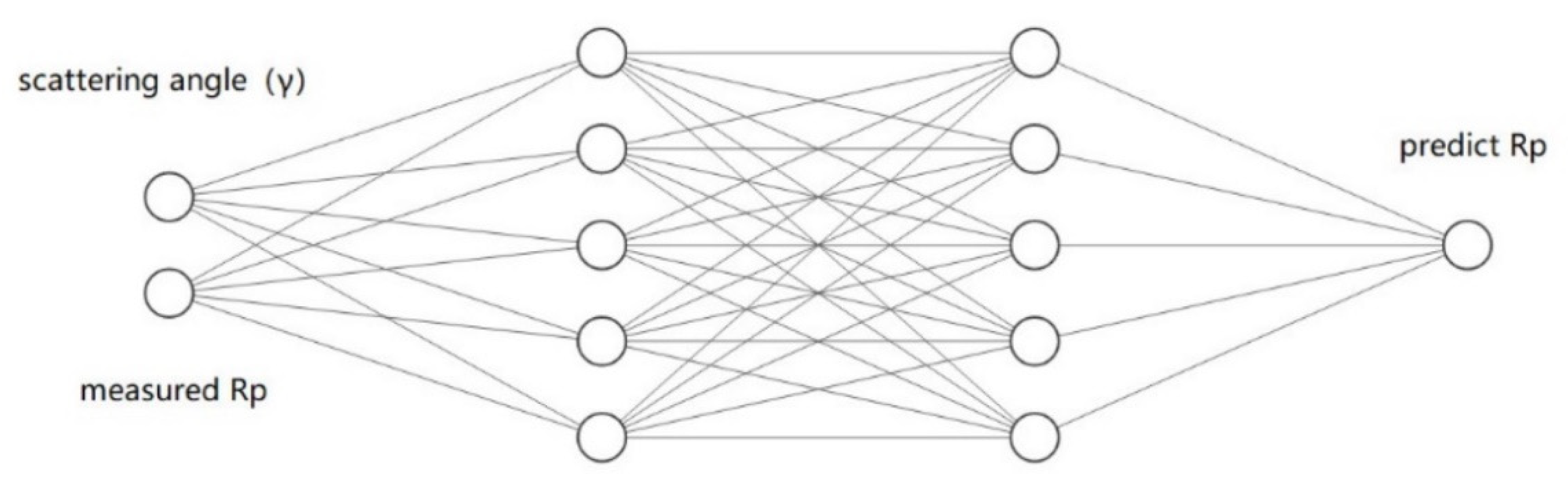
In the deep learning method, the learning rate is a very important parameter. It guides the use of the gradient of the loss function to adjust the hyperparameters of the network weight. This directly affects the quality of the deep learning results. However, the selection of the learning rate value is highly subjective. Depending on the characteristics of the built model, different incoming data, and different research contents, the optimal learning rate of the neural network is also different.

An extremely small or large learning rate may have an unsatisfactory effect. If the learning rate is too low, the final fitting or classification process will be slow. On the other hand, if the learning rate is too high, it may produce loss oscillations or even fail to converge. Therefore, it was particularly important to find a suitable learning rate for the DNN used in this study. However, this experiment lacked the reference of the previous experience; hence, the enumeration method was adopted, that is, the listing of many learning rates and calculating the loss, in order to find the best learning rate.

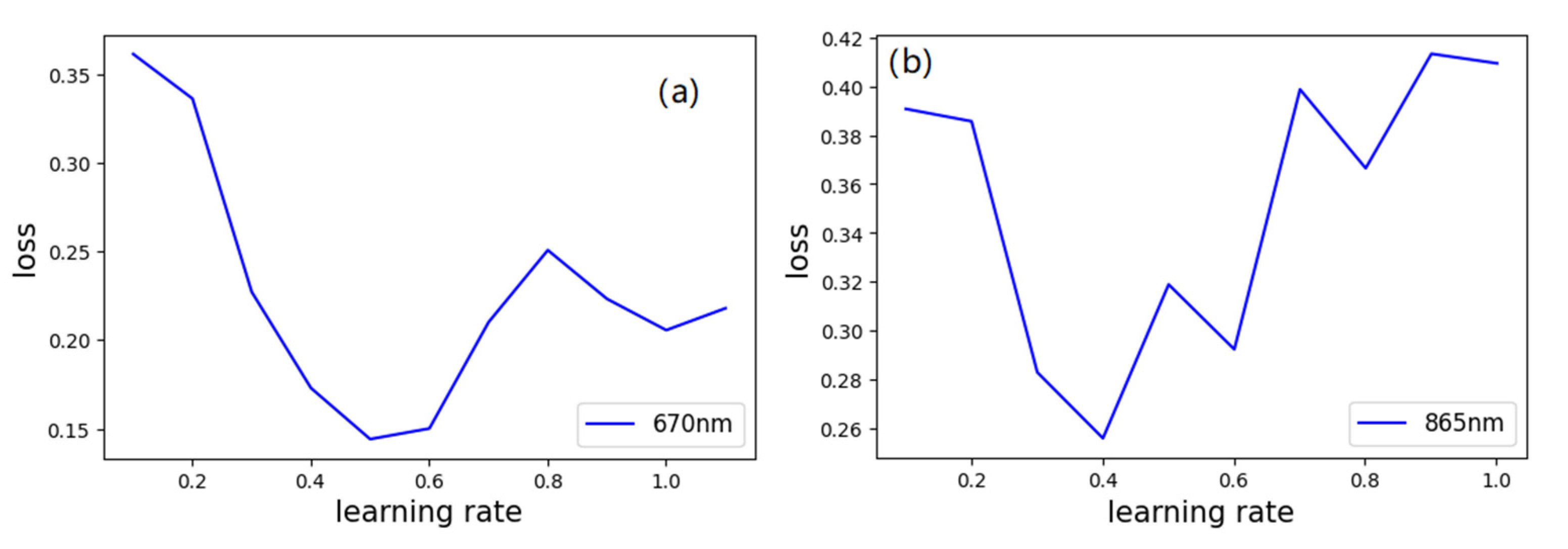
Figure 9a shows the loss results for different learning rates in the 670 nm band, while Figure 9b shows the loss results of different learning rates in the 865 nm band [69]. In Figure 9a, in the 670 nm band, the loss of the learning rate decreases significantly in the range of 0.2 to 0.5, and then, as the learning rate increases, the loss also rises and oscillates significantly, such that the best learning rate is approximately 0.5. In the 865 nm band, the learning rate decreases in the range of 0.2 to 0.4, and the loss increases and oscillates in the subsequent learning rate range, such that the optimal learning rate is approximately 0.4. These two values are relatively close; hence, the learning rate of the deep learning BPDF model in this experiment could be selected as a value between 0.4 and 0.5.

6. Conclusions

This study explored the application of a semi-empirical BPDF model and machine learning-based BPDF model in saline-alkaline soil in the laboratory. The results showed that the six models used in this study, whether the semi-empirical BPDF model or the machine learning-based BPDF model, had relatively good results. However, the machine learning-based BPDF model generally presented better results than the semi-empirical BPDF model. Among these, the deep learning method had the best effect. Therefore, the machine learning method was further discussed, and the influence of different training data ratios and different learning rates on the learning effect under the application of the polarized reflectance of the saline-alkaline soil surface was discussed; the best training ratio and learning rate were determined. The results indicate that the difference in the proportion of training data and the difference in the learning rate has a greater impact on the fitting results. A training data proportion that is too low or too high will reduce the fitting effect. The best training ratio was between 60% and 70%. With a 40% to 30% test set, the best learning rate of the DNN-BPDF model was between 0.4 and 0.5.

In summary, this study explored different types of models for the polarization reflectance of saline-alkaline soils, which is helpful and significant for both the remote sensing investigations of saline-alkaline soils and the study of BPDF models.

References

1. Hassani, A.; Azapagic, A.; Shokri, N. Predicting long-term dynamics of soil salinity and sodicity on a global scale. Proc. Natl. Acad. Sci. USA 2020, 117, 33017–33027. [Google Scholar] [CrossRef]
2. Abrol, I.; Yadav, J.; Massoud, F. Salt-Affected Soils and Their Management; Food & Agriculture Org: Leuven, Belgium, 1988. [Google Scholar]
3. Ginn, F. The International Encyclopedia of Geography: People, The Earth, Environment and Technology; Blackwell Publishing: Boken, NJ, USA, 2017. [Google Scholar] [CrossRef] [Green Version]
4. Daliakopoulos, I.N.; Tsanis, I.K.; Koutroulis, A.; Kourgialas, N.N.; Varouchakis, A.E.; Karatzas, G.P.; Ritsema, C.J. The threat of soil salinity: A European scale review. Sci. Total Environ. 2016, 573, 727–739. [Google Scholar] [CrossRef]
5. Wong, V.N.L.; Greene, R.S.B.; Dalal, R.C.; Murphy, B.W. Soil carbon dynamics in saline and sodic soils: A review. Soil Use Manag. 2010, 26, 2–11. [Google Scholar] [CrossRef]
6. Paix, M.J.D.L.; Lanhai, L.; Xi, C.; Varenyam, A.; Nyongesah, M.J.; Habiyaremye, G. Physicochemical properties of saline soils and aeolian dust. Land Degrad. 2013, 24, 539–547. [Google Scholar] [CrossRef]
7. Singh, K. Microbial and Enzyme Activities of Saline and Sodic Soils. Land Degrad. Dev. 2016, 27, 706–718. [Google Scholar] [CrossRef]
8. Rath, K.M.; Rousk, J. Salt effects on the soil microbial decomposer community and their role in organic carbon cycling: A review. Soil Biol. Biochem. 2015, 81, 108–123. [Google Scholar] [CrossRef]
9. Parihar, P.; Singh, S.; Singh, R.; Singh, V.P.; Prasad, S.M. Effect of salinity stress on plants and its tolerance strategies: A review. Environ. Sci. Pollut. Res. Int. 2015, 22, 4056–4075. [Google Scholar] [CrossRef] [PubMed]
10. Perri, S.; Suweis, S.; Holmes, A.; Marpu, P.R.; Entekhabi, D.; Molini, A. River basin salinization as a form of aridity. Proc. Natl. Acad. Sci. USA 2020, 117, 17635–17642. [Google Scholar] [CrossRef] [PubMed]
11. Kai-shan, S. The Polarized Reflectance Characteristics of Some Soils. Sci. Geogr. Sin. 2004, 24, 357–363. [Google Scholar]
12. Hassani, A.; Azapagic, A.; d Odorico, P.; Keshmiri, A.; Shokri, N. Desiccation crisis of saline lakes: A new decision-support framework for building resilience to climate change. Sci. Total Environ. 2019, 703, 134718. [Google Scholar] [CrossRef] [PubMed]
13. Curran, P. The relationship between polarized visible light and vegetation amount. Remote Sens. Environ. 1981, 11, 87–92. [Google Scholar] [CrossRef]
14. Bradley, C.L.; Diner, D.J.; Xu, F.; Kupinski, M.; Chipman, R.A. Spectral Invariance Hypothesis Study of Polarized Reflectance with the Ground-Based Multiangle SpectroPolarimetric Imager. IEEE Trans. Geosci. Remote Sens. 2019, 57, 8191–8207. [Google Scholar] [CrossRef]
15. Talmage, D.; Curran, P.J. Remote sensing using partially polarized light. Int. J. Remote Sens. 1986, 7, 47–64. [Google Scholar] [CrossRef]
16. Peltoniemi, J.; Järvinen, J.; Zubko, N.; Gritsevich, M. Spectropolarimetric characterization of pure and polluted land surfaces. Int. J. Remote Sens. 2020, 41, 4865–4878. [Google Scholar] [CrossRef]
17. Suomalainen, J.; Hakala, T.; Puttonen, E.; Peltoniemi, J. Polarised bidirectional reflectance factor measurements from vegetated land surfaces. J. Quant. Spectrosc. Radiat. Transf. 2009, 110, 1044–1056. [Google Scholar] [CrossRef]
18. Deuze, J.; Bréon, F.; Devaux, C.; Goloub, P.; Herman, M.; Lafrance, B.; Maignan, F.; Marchand, A.; Nadal, F.; Perry, G.; et al. Remote sensing of aerosols over land surfaces from POLDEr ADEOs 1 polarized measurements. J. Geophys. Res. 2001, 106, 4913–4926. [Google Scholar] [CrossRef] [Green Version]
19. Xie, D.; Cheng, T.; Zhang, W.; Yu, J.; Li, X.; Gong, H. Aerosol type over east Asian retrieval using total and polarized remote Sensing. J. Quant. Spectrosc. Radiat. Transf. 2013, 129, 15–30. [Google Scholar] [CrossRef]
20. Wang, H.; Yang, L.K.; Zhao, M.R.; Du, W.B.; Liu, P.; Sun, X.B. The Normalized Difference Vegetation Index and Angular Variation of Surface Spectral Polarized Reflectance Relationships: Improvements on Aerosol Remote Sensing Over Land. Earth Space Sci. 2019, 6, 982–989. [Google Scholar] [CrossRef] [Green Version]
21. Nadal, F.; Bréon, F.M. Parameterization of surface polarized reflectance derived from POLDER spaceborne measurements. IEEE Trans. Geosci. Remote Sens. 1999, 37, 1709–1718. [Google Scholar] [CrossRef]
22. Maignan, F.; Bréon, F.; Fedele, E.; Bouvier, M.J.R.S.o.E. Polarized reflectances of natural surfaces: Spaceborne measurements and analytical modeling. Remote Sens. Environ. 2009, 113, 2642–2650. [Google Scholar] [CrossRef]
23. Yang, B.; Zhao, H.M.; Chen, W. Modeling polarized reflectance of snow and ice surface using POLDER measurements. J. Quant. Spectrosc. Radiat. Transf. 2019, 236, 106578. [Google Scholar] [CrossRef]
24. Martin, W.E.; Hesse, E.; Hough, J.H.; Sparks, W.B.; Cockell, C.S.; Ulanowski, Z.; Germer, T.A.; Kaye, P.H. Polarized optical scattering signatures from biological materials. J. Quant. Spectrosc. Radiat. Transf. 2010, 111, 2444–2459. [Google Scholar] [CrossRef] [Green Version]
25. Sun, Z.Q.; Wu, D.; Lv, Y.F.; Lu, S. Optical Properties of Reflected Light from Leaves: A Case Study from One Species. IEEE Trans. Geosci. Remote Sens. 2019, 57, 4388–4406. [Google Scholar] [CrossRef]
26. Nilson, T.; Kuusk, A. A reflectance model for the homogeneous plant canopy and its inversion. Remote Sens. Environ. 1989, 27, 157–167. [Google Scholar] [CrossRef]
27. Rondeaux, G.; Herman, M. Polarization of light reflected by crop canopies. Remote Sens. Environ. 1991, 38, 63–75. [Google Scholar] [CrossRef]
28. Sun, Z.Q.; Huang, Y.H.; Bao, Y.L.; Wu, D. Polarized Remote Sensing: A Note on the Stokes Parameters Measurements from Natural and Man-Made Targets Using a Spectrometer. IEEE Trans. Geosci. Remote Sens. 2017, 55, 4008–4021. [Google Scholar] [CrossRef]
29. Grant, L.; Daughtry, C.S.T.; Vanderbilt, V.C. Polarized and Specular Reflectance Variation with Leaf Surface-Features. Physiologia Plantarum 1993, 88, 1–9. [Google Scholar] [CrossRef]
30. Yang, B.; Knyazikhin, Y.; Lin, Y.; Yan, K.; Chen, C.; Park, T.; Choi, S.; Mottus, M.; Rautiainen, M.; Myneni, R.B.; et al. Analyses of Impact of Needle Surface Properties on Estimation of Needle Absorption Spectrum: Case Study with Coniferous Needle and Shoot Samples. Remote Sens. 2016, 8, 563. [Google Scholar] [CrossRef] [Green Version]
31. Breon, F.M.; Tanre, D.; Lecomte, P.; Herman, M. Polarized Reflectance of Bare Soils and Vegetation—Measurements and Models. IEEE Trans. Geosci. Remote Sens. 1995, 33, 487–499. [Google Scholar] [CrossRef]
32. Litvinov, P.; Hasekamp, O.; Cairns, B.; Mishchenko, M. Reflection models for soil and vegetation surfaces from multiple-viewing angle photopolarimetric measurements. J. Quant. Spectrosc. Radiat. Transf. 2010, 111, 529–539. [Google Scholar] [CrossRef]
33. Xie, D.; Cheng, T.; Wu, Y.; Fu, H.; Zhong, R.; Yu, J. Polarized reflectances of urban areas: Analysis and models. Remote Sens. Environ. 2017, 193, 29–37. [Google Scholar] [CrossRef]
34. Peltoniemi, J.I.; Gritsevich, M.; Hakala, T.; Dagsson-Waldhauserova, P.; Arnalds, O.; Anttila, K.; Hannula, H.R.; Kivekas, N.; Lihavainen, H.; Meinander, O.; et al. Soot on Snow experiment: Bidirectional reflectance factor measurements of contaminated snow. Cryosphere 2015, 9, 2323–2337. [Google Scholar] [CrossRef] [Green Version]
35. Yang, B.; Zhao, H.M.; Chen, W. Semi-empirical models for polarized reflectance of land surfaces: Intercomparison using space-borne POLDER measurements. J. Quant. Spectrosc. Radiat. Transf. 2017, 202, 13–20. [Google Scholar] [CrossRef]
36. Vanderbilt, V.; Grant, L.J.I.T.o.G.; Sensing, R. Plant Canopy Specular Reflectance Model. IEEE Trans. Geosci. Remote Sens. 1985, GE-23, 722–730. [Google Scholar] [CrossRef]
37. Diner, D.J.; Xu, F.; Martonchik, J.V.; Rheingans, B.E.; Geier, S.; Jovanovic, V.M.; Davis, A.; Chipman, R.A.; McClain, S.C. Exploration of a Polarized Surface Bidirectional Reflectance Model Using the Ground-Based Multiangle SpectroPolarimetric Imager. Atmosphere 2012, 3, 591–619. [Google Scholar] [CrossRef] [Green Version]
38. Waquet, F.; Leon, J.F.; Cairns, B.; Goloub, P.; Deuze, J.L.; Auriol, F. Analysis of the spectral and angular response of the vegetated surface polarization for the purpose of aerosol remote sensing over land. Appl. Opt. 2009, 48, 1228–1236. [Google Scholar] [CrossRef] [PubMed]
39. Litvinov, P.; Hasekamp, O.; Cairns, B. Models for surface reflection of radiance and polarized radiance: Comparison with airborne multi-angle photopolarimetric measurements and implications for modeling top-of-atmosphere measurements. Remote Sens. Environ. 2011, 115, 781–792. [Google Scholar] [CrossRef]
40. He, Y.H.; Yang, B.; Lin, H.; Zhang, J.Q. Modeling Polarized Reflectance of Natural Land Surfaces Using Generalized Regression Neural Networks. Remote Sens. 2020, 12, 248. [Google Scholar] [CrossRef] [Green Version]
41. Gilichinsky, M.; Heiskanen, J.; Barth, A.; Wallerman, J.; Egberth, M.; Nilsson, M. Histogram matching for the calibration of kNN stem volume estimates. Int. J. Remote Sens. 2012, 33, 7117–7131. [Google Scholar] [CrossRef]
42. Ichii, K.; Ueyama, M.; Kondo, M.; Saigusa, N.; Kim, J.; Alberto, M.C.; Ardo, J.; Euskirchen, E.S.; Kang, M.; Hirano, T.; et al. New data-driven estimation of terrestrial CO2 fluxes in Asia using a standardized database of eddy covariance measurements, remote sensing data, and support vector regression. J. Geophys. Res. Biogeosci. 2017, 122, 767–795. [Google Scholar] [CrossRef]
43. Shah, S.H.; Angel, Y.; Houborg, R.; Ali, S.; McCabe, M.F. A Random Forest Machine Learning Approach for the Retrieval of Leaf Chlorophyll Content in Wheat. Remote Sens. 2019, 11, 920. [Google Scholar] [CrossRef] [Green Version]
44. Maxwell, A.E.; Warner, T.A.; Fang, F. Implementation of machine-learning classification in remote sensing: An applied review. Int. J. Remote Sens. 2018, 39, 2784–2817. [Google Scholar] [CrossRef] [Green Version]
45. Zerrouki, N.; Harrou, F.; Sun, Y.; Hocini, L. A Machine Learning-Based Approach for Land Cover Change Detection Using Remote Sensing and Radiometric Measurements. IEEE Sens. J. 2019, 19, 5843–5850. [Google Scholar] [CrossRef] [Green Version]
46. Liang, L.; Di, L.P.; Zhang, L.P.; Deng, M.X.; Qin, Z.H.; Zhao, S.H.; Lin, H. Estimation of crop LAI using hyperspectral vegetation indices and a hybrid inversion method. Remote Sens. Environ. 2015, 165, 123–134. [Google Scholar] [CrossRef]
47. Loozen, Y.; Rebel, K.T.; de Jong, S.M.; Lu, M.; Ollinger, S.V.; Wassen, M.J.; Karssenberg, D. Mapping canopy nitrogen in European forests using remote sensing and environmental variables with the random forests method. Remote Sens. Environ. 2020, 247, 111933. [Google Scholar] [CrossRef]
48. Feret, J.B.; le Maire, G.; Jay, S.; Berveiller, D.; Bendoula, R.; Hmimina, G.; Cheraiet, A.; Oliveira, J.C.; Ponzoni, F.J.; Solanki, T.; et al. Estimating leaf mass per area and equivalent water thickness based on leaf optical properties: Potential and limitations of physical modeling and machine learning. Remote Sens. Environ. 2019, 231, 110959. [Google Scholar] [CrossRef]
49. Liu, S.; Lin, Y.; Yan, L.; Yang, B. Modeling Bidirectional Polarization Distribution Function of Land Surfaces Using Machine Learning Techniques. Remote Sens. 2020, 12, 3891. [Google Scholar] [CrossRef]
50. Belgiu, M.; Dragut, L. Random forest in remote sensing: A review of applications and future directions. ISPRS J. Photogramm. 2016, 114, 24–31. [Google Scholar] [CrossRef]
51. Grafton, R.; Nelson, H.; Lambie, N.R.; Wyrwoll, P.R. Normalized Difference Vegetation Index (NDVI): Unforeseen successes in animal ecology. Clim. Res. 2012, 46, 15–27. [Google Scholar] [CrossRef]
52. Goodfellow, I.; Bengio, Y.; Courville, A.C. Deep Learning. Nature 2015, 521, 436–444. [Google Scholar] [CrossRef]
53. Krizhevsky, A.; Sutskever, I.; Hinton, G.E. ImageNet classification with deep convolutional neural networks. Commun. ACM 2012, 60, 84–90. [Google Scholar] [CrossRef]
54. Chai, T.; Draxler, R.R. Root mean square error (RMSE) or mean absolute error (MAE)?—Arguments against avoiding RMSE in the literature. Geosci. Model Dev. 2014, 7, 1247–1250. [Google Scholar] [CrossRef] [Green Version]
55. Xu, Y.; Wang, L.; Ma, Z.; Li, B.; Bartels, R.; Liu, C.; Zhang, X.; Dong, J. Spatially Explicit Model for Statistical Downscaling of Satellite Passive Microwave Soil Moisture. IEEE Trans. Geosci. Remote Sens. 2020, 58, 1182–1191. [Google Scholar] [CrossRef]
56. Lin, L. A concordance correlation coefficient to evaluate reproducibility. Biometrics 1989, 45, 255–268. [Google Scholar] [CrossRef]
57. Archdeacon, T.J. Correlation and Regression Analysis: A Historian’s Guide; University of Wisconsin Press: Madison, WI, USA, 1994. [Google Scholar]
58. Brown, C.E. Coefficient of variation. In Applied Multivariate Statistics in Geohydrology and Related Sciences; Springer: Berlin/Heidelberg, Germany, 1998; pp. 155–157. [Google Scholar]
59. Wang, Z.M.; Song, K.S.; Zhang, B.; Liu, D.W.; Ren, C.Y.; Luo, L.; Yang, T.; Huang, N.; Hu, L.; Yang, H.J.; et al. Shrinkage and fragmentation of grasslands in the West Songnen Plain, China. Agric. Ecosyst. Environ. 2009, 129, 315–324. [Google Scholar] [CrossRef]
60. He, J.; Gao, C.; Lin, Q.; Zhang, S.; Zhao, W.; Lu, X.; Wang, G. Temporal and Spatial Changes in Black Carbon Sedimentary Processes in Wetlands of Songnen Plain, Northeast of China. PLoS ONE 2015, 10, e0140834. [Google Scholar] [CrossRef] [PubMed] [Green Version]
61. Ren, J.H.; Li, X.J.; Zhao, K. Quantitative analysis of relationships between crack characteristics and properties of soda-saline soils in Songnen Plain, China. Chin. Geogr. Sci. 2015, 25, 591–601. [Google Scholar] [CrossRef]
62. Liu, Q.; Cui, B.S.; Yang, Z.F. Dynamics of the soil water and solute in the sodic saline soil in the Songnen Plain, China. Environ. Earth Sci. 2009, 59, 837–845. [Google Scholar] [CrossRef]
63. Yang, X.G.; Yu, Y. Estimating Soil Salinity Under Various Moisture Conditions: An Experimental Study. IEEE Trans. Geosci. Remote Sens. 2017, 55, 2525–2533. [Google Scholar] [CrossRef]
64. Xiu, L. The Alkili-saline Land and Agricultural Sustainable Development of the Western Songnen Plain in China. Sci. Geogr. Sin. 2000, 20, 51–55. [Google Scholar]
65. Drake, N.A. Reflectance Spectra of Evaporite Minerals (400-2500-Nm)—Applications for Remote-Sensing. Int. J. Remote Sens. 1995, 16, 2555–2571. [Google Scholar] [CrossRef]
66. Crowley, J.K. Visible and near-infrared (0.4-2.5μm) reflectance spectra of Playa evaporite minerals. J. Geophys. Res. 1991, 96, 16231–16240. [Google Scholar] [CrossRef]
67. Weng, Y.L.; Gong, P.; Zhu, Z.L. Reflectance spectroscopy for the assessment of soil salt content in soils of the Yellow River Delta of China. Int. J. Remote Sens. 2008, 29, 5511–5531. [Google Scholar] [CrossRef]
68. Salazar, A.; Vergara, L.; Safont, G. Generative Adversarial Networks and Markov Random Fields for oversampling very small training sets. Expert Syst. Appl. 2021, 163, 113819. [Google Scholar] [CrossRef]
69. Smith, L.N. Cyclical Learning Rates for Training Neural Networks. In Proceedings of the 2017 IEEE Winter Conference on Applications of Computer Vision (WACV), Santa Rosa, CA, USA, 24–31 March 2017; pp. 464–472. [Google Scholar]
Figure 1. Schematic diagram of the operation of the semi-empirical BPDF model.
Remotesensing 14 00226 g001
Figure 2. Schematic diagram of the DNN model.
Remotesensing 14 00226 g002
Figure 3. Schematic diagram of the Rp inversion process of the BPDF model based on the machine learning method.
Remotesensing 14 00226 g003
Figure 4. Latitude and longitude coordinates of the soil field collection site, and its relative position in China.
Remotesensing 14 00226 g004
Figure 5. The schematic diagram of the experimental process. In it, the azimuth angle is the circumferential direction. The zenith angle is the radial direction. The saline-alkaline soil sample is placed in the center of the circle. The solar azimuth angle is 0°, and the solar zenith angle is 40°. The position of the detector changes with the azimuth angle and the zenith angle.
Remotesensing 14 00226 g005
Figure 6. Spectra of BPDF measured on the surface of saline-alkaline soil: (a) is the spectra of different detection angles at an azimuth of 0; (b) is the spectrum of different azimuth angles at a 20° detection angle.
Remotesensing 14 00226 g006
Figure 7. Fitting situation of the surface Rp of saline-alkaline soil predicted by the semi-empirical BPDF model and the actual measured Rp (a) 670 nm Nadal–Bréon model, (b) 865 nm Nadal–Bréon model, (c) 670 nm Litvinov model, (d) 865 nm Litvinov model, (e) 670 nm Xie–Cheng model, and (f) 865 nm Xie–Cheng model.
Remotesensing 14 00226 g007
Figure 8. Fitting situation of the surface Rp of saline-alkaline soil predicted by the BPDF model, based on machine learning methods and the actual measured Rp. (a) 670 nm SVR, (b) 865 nm SVR, (c) 670 nm RF, (d) 865 nm RF, (e) 670 nm DNN, and (f) 865 nm DNN.
Remotesensing 14 00226 g008
Figure 9. Loss results of different bands and different learning rates, applied to DNN. (a,b) respectively represent the results of 670 nm and 865 nm bands.
Remotesensing 14 00226 g009