Mapping Blue and Red Color-Coated Steel Sheet Roof Buildings over China Using Sentinel-2A/B MSIL2A Images

Abstract

Accurate and efficiently updated information on color-coated steel sheet (CCSS) roof materials in urban areas is of great significance for understanding the potential impact, challenges, and issues of these materials on urban sustainable development, human health, and the environment. Thanks to the development of Earth observation technologies, remote sensing (RS) provides abundant data to identify and map CCSS materials with different colors in urban areas. However, existing studies are still quite challenging with regards to the data collection and processing costs, particularly in wide geographical areas. Combining free access high-resolution RS data and a cloud computing platform, i.e., Sentinel-2A/B data sets and Google Earth Engine (GEE), this study aims at CCSS material identification and mapping. Specifically, six novel spectral indexes that use Sentinel-2A/B MSIL2A data are proposed for blue and red CCSS material identification, namely the normalized difference blue building index (NDBBI), the normalized difference red building index NDRBI, the enhanced blue building index (EBBI), the enhanced red building index (ERBI), the logical blue building index (LBBI) and the logical red building index (LRBI). These indexes are qualitatively and quantitatively evaluated on a very large number of urban sites all over the P.R. China and compared with the state-of-the-art redness and blueness indexes (RI and BI, respectively). The results demonstrate that the proposed indexes, specifically the LRBI and LBBI, are highly effective in visual evaluation, clearly detecting and discriminating blue and red CCSS covers from other urban materials. Results show that urban areas from the northern parts of P.R. China have larger proportions of blue and red CCSS materials, and areas of blue and red CCSS material buildings are positively correlated with population and urban size at the provincial level across China.

1. Introduction

Over the last few decades, the Earth’s surface has experienced dramatic changes due, among other reasons, to rapid urbanization. This process is expected to continue for the rest of the 21st century, particularly for developing countries in Asia and Africa [1]. Today, more than 55% of the world population lives in towns and cities, which only occupy less than 0.60% of the global land surface, and by 2030 the number of the world urban population will swell to approximately 8.6 billion, more than 70% of the world population [2,3,4,5]. Along with this trend of global urbanization, the global urban area is expected to increase by roughly 40–67% until 2050 relative to the base year of 2013, with a growth ratio of more than 200% by the year 2100 [1,6].

As one of the key elements in the process of development, urbanization has provided more and better living environments for more people worldwide and boosted economic developments, particularly for developing countries [7,8,9,10,11]. However, urbanization is also one of two major global environmental concerns of the 21st century [12,13], mainly because urban expansion has posed a wide range of challenges and issues to the social-economic, ecology, and environment at regional, national and global scales [1,6,14,15,16,17,18,19,20,21]. To mitigate potential risks and overcome issues caused by rapid urban expansion, it is of crucial importance to understand the pathways of urban growth. Thereby, numerous works have been documented with the subject of urban land cover or land use [22,23], urban extents [24,25], urban built-up areas [26,27,28], urban impervious surfaces [5,29,30], urban dynamics [20], urban nighttime lights [4,31,32,33], urban energy consumption [34,35], urban growth simulation and modeling [1,6,10,36,37], and so on.

Impacts, challenges, and issues following the trend of urban expansion are not only related to urban population density, urban area size and structure in both horizontal and vertical dimensions, environmental carrying capacity, geography and climatology background, water and land resources, planning and managing policy but they are also related to urban building types, patterns, and materials [38,39,40,41,42,43,44,45,46]. Hence, urban building extraction, building type identification, and pattern analysis are very important research topics with respect to both aspects of algorithmic and application studies in the field of urban remote sensing (URS) [47,48,49,50,51,52].

Specifically, building materials have significant impacts on urban energy consumption and flux by influencing electromagnetic (absorption, reflectivity, and emissivity) and electrochemistry properties of the built-up structures. They also influence building quality, safety, and serviceability, maintainability, and sustainability [44,53,54,55,56,57,58,59,60]. So far, in technical literature, only a few works have focused on building materials identification and building extraction with specific material using remote sensing (RS) imageries, and these works were carried out in small test areas [61,62,63,64]. This is mainly due to the fact that urban building materials have a great variety of types (e.g., woods, tiles, bricks, concrete, plastics, glass, metals, composites, and their combinations) with complex and diverse physicochemical properties and very complex geometrical shapes and structures.

Thanks to the development of Earth observation technologies, now urban building material types can be identified using hyperspectral, synthetic aperture radar (SAR), polarimetric SAR (PolSAR), light detection and ranging (LiDAR), and high or very high-resolution (HR/VHR) multispectral instruments, capable of capturing information about physicochemical and geometrical properties [61,64,65,66]. However, challenging issues still remain open. For instance, spaceborne hyperspectral and LiDAR images have low and mid-spatial resolution and cannot capture detailed geometrical information about urban building materials. Spaceborne and airborne VHR visible and infrared images, as well as airborne LiDAR data, cannot provide sufficient spectral information about physicochemical properties of building materials [67,68,69]. SAR and PolSAR images, especially at high and very high spatial resolutions, suffer from speckle noise, and geometrical distortion effects become serious in areas with tall and dense buildings [70,71,72]. Because of these limitations, jointly using multispectral and hyperspectral images with HR and VHR spatial resolution, LiDAR data with HR and VHR spatial resolution, and multispectral images seem to be a possible solution. Still, these ideas are quite challenging to be implemented in wide geographical areas because of the heterogeneity between data sets and the data collection costs, hampering their usefulness in regional, national and global scale analysis scenarios. Hence, it is worth using more advanced but free accessible data sets on a cloud computing platform for urban building material identification in these scenarios.

As an easily accessible and user-friendly cloud-based platform for planetary-scale geospatial data processing with massive computational capabilities, Google Earth Engine (GEE) has been in the big RS data processing and application spotlight in recent years [73,74]. The current GEE’s open-source data catalog not only includes petabyte scales of over 40 years of RS data but also includes unprecedented volumes of geographic information system (GIS)-based vector data sets, climate, weather, social, demographic, geophysical, and ready-to-use products data layers [75]. Additionally, it provides a library of application programming interfaces (APIs) with a full-featured development environment for JavaScript and Python and an associated web-based interactive development environment (IDE) to interact with users. Owing to these advantages, GEE has led researchers to harness it for various applications, such as water, vegetation, ecosystem and biodiversity, natural hazards, agricultural, hydrology, urban, land cover, and many others [76,77,78,79].

Therefore, in this work, we focus on Sentinel-2A/B images with four bands at 10 m spatial resolution for specific material building identification and mapping over China using the GEE platform to detect color-coated steel sheets (CCSS). The contribution of urbanization to economic growth mainly comes from the construction industry and industrialization process that always have massive demands for construction materials. CCSS is composed of color-painted and galvanized steel plate surfaces with a polystyrene foam plastic sandwich layer [80]. In contrast with traditional roof materials such as wood, tiles, bricks, and concrete, CCSS has the properties of being lightweight, artistic, heat-insulation, soundproof, anti-corrosive, durable, stiff, easy to manufacture, and most importantly, it has a much lower market price. According to the CCSS industry and market search report of China for 2020, there were more than 13000 enterprises that produced more than 12 million tons of CCSS materials in 2019, and the value of the CCSS exchanging market was more than 70 billion RMB [81].

Nowadays, CCSS sheets are commonly found in urban areas, particularly on buildings for warehouses, stations, airport terminals, factories, logistic parks, supermarkets, stadiums, construction sites, vegetable greenhouses, farms, carports, dovecotes, as well as commercial and residential houses (Figure 1). Due to their easiness to manufacture and lower market price, CCSS sheets are mostly used for houses in shantytowns, as well as non-compliance and even illegal rooftop remodeling in downtown areas (Figure 1g). Despite the advanced properties mentioned earlier, CCSS materials may cause issues related to safety, serviceability, maintainability, and sustainability [58,82,83,84].

Additionally, from the eco-city planning and construction, urban and building color planning and design, urban ecological and environmental aesthetics, and bird-friendly urban color environment points of view, massively using CCSS materials in urban buildings is not the best option [7,85,86,87,88]. For instance, CCSS material can significantly impact local surface heat and urban energy consumption and flux by influencing electromagnetic absorption, reflectivity, and emissivity of the buildings. Thus, identifying and locating buildings covered with CCSS is an important task. To date, only a few works have focused on the CCSS material detection, mapping, and spatial pattern analysis in urban areas [89,90].

Generally, CCSS materials can be painted in any color. However, since red mineral pigment is much cheaper than other ones, and blue color has better stability, and both red and blue CCSS materials have better thermal keeping capabilities than other colors. CCSS sheets with these two colors are much more commonly used in the construction industry. Thereby, most of the works of CCSS building identification and locating are focused on the red and blue CCSS material using supervised classification, object-oriented segmentation, and spectral matching methods [65,66,83,89,90]. It should be noted, however, that these somehow conventional approaches are labor intensive, inefficient, and impractical because of the material and urban landscape heterogeneity at large scales. Therefore, there is a great demand for methods that would allow for accurate and efficient up-to-date mapping of CCSS material buildings’ spatial distribution in single urban areas, at regional and even national scales.

In this study, Sentinel-2A/B MSIL2A images are used to develop several spectral indexes to enhance, identify and map blue and red CCSS sheets all over China, whose performance is comprehensively evaluated. Additionally, a detailed correlation between the CCSS sheet total area and the urban population is performed and discussed.

2. Study Area and Materials

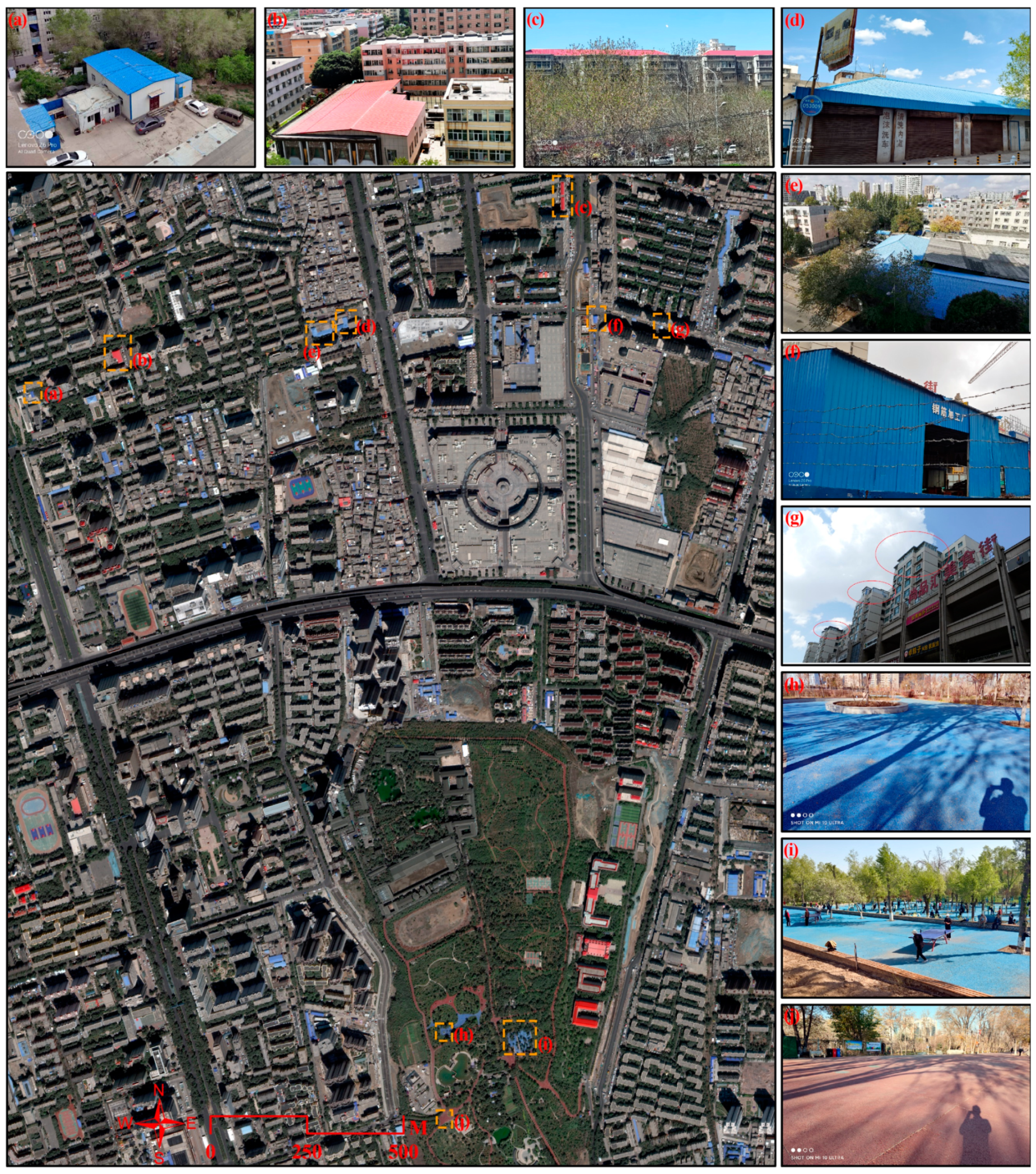
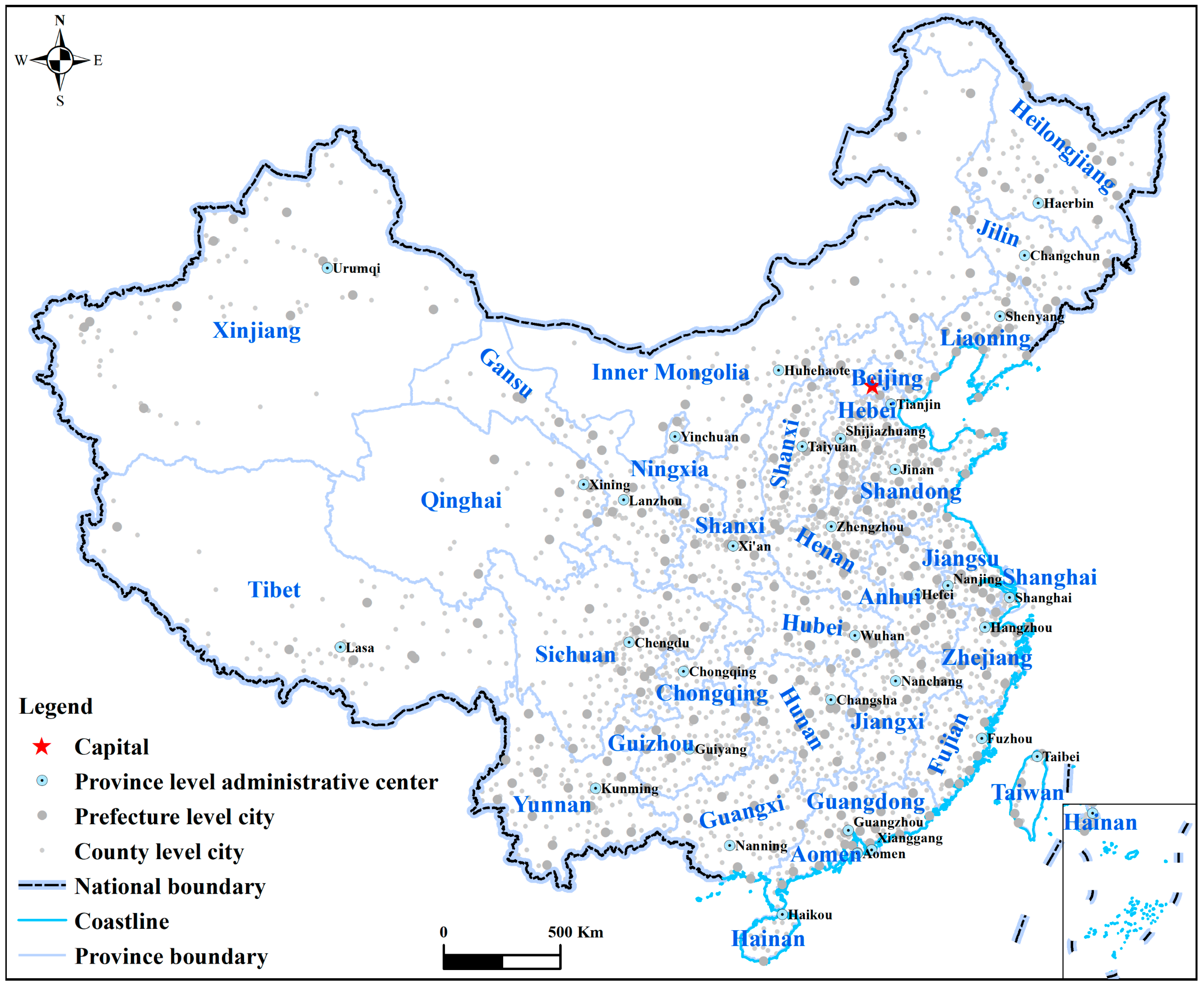
2.1. Study Area

The study area in this paper is the whole of P.R. China, which has experienced dramatic land changes due to an extremely rapid urbanization process in the past several decades, and it is currently the world’s most populous country with an uneven process of development and urbanization across the country. Before mapping blue and red CCSS roof buildings, performances of the proposed method need to be proved by enough experiments using both qualitative and quantitative measures. To this aim, we selected 32 test sites all over the world representing a variety of locations, landscapes, city sizes, and urbanization levels to assess the proposed methods. As detailed in Figure 2 and

Table 1. Detailed information for the selected test sites.

Site No.	Country	City Name	Scene Center Location		Spacecraft Name	Orbit Number	Sensing Time
			Latitude	Longitude
1	China	Urumqi	43°43′24″	87°35′20″	Sentinel-2A	19	2020-10-15T08:04:29
2	China	Urumqi	43°55′2″	87°21′60″	Sentinel-2A	19	2020-10-15T08:04:29
3	China	Urumqi	43°50′25″	87°18′17″	Sentinel-2A	19	2020-10-15T08:04:29
4	China	Urumqi	43°43′57″	87°22′12″	Sentinel-2A	19	2020-10-15T08:04:29
5	China	Chuzhou	32°18′57″	118°23′10″	Sentinel-2A	132	2019-09-19T08:23:30
6	China	Haerbin	45°37′12″	126°37′14″	Sentinel-2A	89	2020-10-20T05:26:23
7	China	Hefei	31°41′49″	117°11′33″	Sentinel-2A	132	2020-10-23T05:38:54
8	China	Tianjin	39°21′8″	117°43′40″	Sentinel-2B	32	2020-09-01T05:56:11
9	China	Tianjin	39°16′49″	117°49′24″	Sentinel-2B	32	2020-09-01T05:56:11
10	China	Xining	36°41′43″	101°44′56″	Sentinel-2A	4	2020-04-27T08:09:55
11	China	Changchun	43°54′2″	125°26′42″	Sentinel-2A	89	2020-10-20T05:26:23
12	China	Yinchuan	38°27′33″	106°6′32″	Sentinel-2A	104	2020-05-14T08:36:42
13	China	Shihezi	44°25′56″	86°5′14″	Sentinel-2B	19	2020-07-22T09:30:27
14	China	Shenyang	41°57′2″	123°32′56″	Sentinel-2B	89	2020-06-07T05:18:53
15	China	Shenyang	41°45′46″	123°14′23″	Sentinel-2B	89	2020-06-07T05:18:53
16	China	Shijiazhuang	38°4′29″	114°2′10″	Sentinel-2A	75	2020-09-19T06:06:33
17	Iran	Tehran	35°27′41″	51°21′46″	Sentinel-2B	6	2020-09-19T09:56:38
18	Iran	Caspian Industral Twon	36°11′9″	50°16′47″	Sentinel-2A	6	2020-10-24T09:47:55
19	Kazakhstan	Nursurtan	51°10′17″	71°31′6″	Sentinel-2A	34	2020-10-16T08:53:32
20	South Korea	Pusan	128°51′22″	35°05′45″	Sentinel-2A	103	2020-04-24T02:07:01
21	South Korea	Inchon	126°37′23″	37°32′52″	Sentinel-2A	3	2020-10-24T04:59:15
22	Maynmaer	Yangon	96°17′28″	16°50′17″	Sentinel-2A	4	2020-12-13T04:01:51
23	Malaysia	Kuala Lumpur	2°57′24″	101°19′37″	Sentinel-2A	18	2020-02-28T07:41:37
24	Cambodia	Phnom Penh	11°27′53″	104°54′15″	Sentinel-2A	118	2019-12-07T07:19:12
25	Vietnam	Ho Chi Minh City	106°28′43″	10°46′44″	Sentinel-2A	118	2020-01-21T03:20:39
26	South Africa	Pretoria	−25°49′15″	28°11′41″	Sentinel-2A	135	2020-10-23T10:15:14
27	Rwanda	Kigali	−1°57′3.85″	30°9′27.27″	Sentinel-2A	78	2019-09-15T08:06:11
28	Lesotho	Maseru	−29°19′48.12″	27°28′3″	Sentinel-2A	135	2020-09-13T10:23:18
29	Zimbabwe	Harare	−17°50′12.58″	27°28′2.74″	Sentinel-2A	135	2020-10-28T07:50:29
30	Kenya	Nairobi	−1°20′7″	36°53′12″	Sentinel-2B	92	2020-10-05T10:20:29
31	Ethiopia	Addis Ababa	8°46′1″	38°55′42″	Sentinel-2B	92	2020-01-19T10:14:10
32	Uganda	Kampala	0°21′21″	32°49′23″	Sentinel-2A	35	2019-12-31T10:42:04

, a total of 16 sites were selected from 11 provinces and counties across mainland China, 9 sites across Northeast, Central, Western, and Southeast Asia, and finally, 7 sites were selected across Eastern and Southern Africa.

2.2. Materials

Sentinel-2 mission is a constellation of twin polar-orbiting satellites (Sentinel-2A and Sentinel-2B) developed and operated by European Space Agency (ESA) [91]. Both Sentinel-2A and Sentinel-2B carry the state-of-the-art multispectral instrument (MSI) sensor that offers spectral bands spanning from the visible (VIS) and the near infrared (NIR) to the short wave infrared (SWIR) at different spatial resolutions at the ground, ranging from 10 to 60 m. By sharing the same sun-synchronous orbit at an altitude of ~786 km but separated by 180°, Sentinel-2A/B can provide better than a 5-day revisit of the Earth’s land surface with an equatorial overpass time at approximately 10:30 a.m. All the Sentinel-2 data used in this study are level-2A (L2A) bottom of atmosphere (BOA) corrected reflectance products, which means per-pixel radiometric measurements are provided in surface reflectance with all parameters to transform them into radiance. Only the visual bands of blue (band 2), green (band 3), red (band 4), and the near-infrared (band 8) with 10 m spatial resolution were used in this study. All images of the selected test sites in Table 1 were processed using the Sentinel Application Platform (SNAP, v8.0), which is a free, open-source software program that is distributed by the ESA-ESRIN (Frascati, Rom, Italy) under the GNU General Public License and funded through the ESA Scientific Exploration of Operational Missions (SEOM) Program.

The urban class from the global land cover with fine classification system at 30 m in 2020 product (GCL-FCS30-2020) [92]) and Global Human Settlements from Sentinel-2 satellite imagery using convolutional neural networks (GLS-S2Net-2018) product [93] were selected to discard the areas outside human settlements.

3. Methods

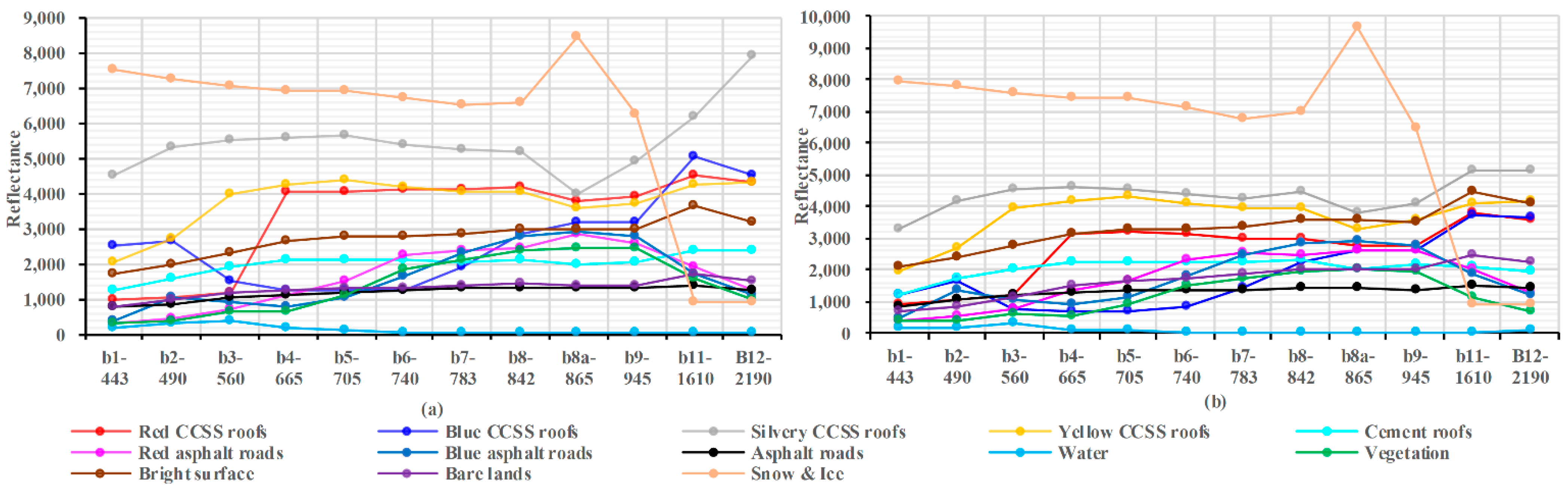
3.1. Spectral Analysis and Normalized Difference Indexes Development

To extract and map blue and red CCSS material buildings in an accurate, fast and unsupervised manner, it is important to analyze and understand the spectral properties of the CCSS materials. To this aim, Figure 3 presents Sentinel-2A average image spectra of blue and red CCSS materials and other land cover types collected around carp fish mountain park at Urumqi City, Xinjiang, China.

According to the graphs in Figure 3, it can be observed that the spectral responses of different CCSS materials are highly variable with respect to both reflectance patterns and magnitudes. For instance, red CCSS material roofs have a nearly flat spectral curve between the wavelength of 443–560 nm and 665–945 nm and have two absorption valleys at the spectral range of red to green (560–565 nm) and water vapor to SWIR (945–1610 nm), which have the potential to distinguish them from other roof types. Compared with the first absorption value, the absorption valley at the spectral range of 945–1610 nm has smoother slopes and overlaps less with the absorption valleys of yellow CCSS roofs, silvery CCSS roofs, bright surfaces, and blue CCSS roofs. Additionally, considering that bands in the spectral range of 560–565 have a higher spatial resolution (10 m) than the bands in the spectral range of 945–1610 (20 m, 60 m), the absorption valley at 560–565 nm has better potential to detect red CCSS materials. Hence, following the simplicity of normalized difference indexes such as the normalized difference vegetation index (NDVI) and the normalized difference water index (NDWI) [94,95], an option would be to define a normalized difference red building index (NDRBI) as follow:

$$\mathrm{NDRBI}=\frac{{\beta }_4-{\beta }_3}{{\beta }_4+{\beta }_3}$$

(1)

where ${\beta }_3$ and ${\beta }_4$ represent the third (green) and fourth (red) Sentinel 2-A/B spectral bands.

Looking now at the spectral reflectance shown by the square marked blue line, the blue CCSS material has a nearly flat spectral curve between in the wavelength of 560–740 nm and two absorption valleys in the spectral ranges of 490–560 nm and 945–1160 nm, which also may have potential to distinguish blue CCSS material from others. However, the latter absorption valley almost overlaps with the absorption valleys of other bright surfaces, such as silvery red CCSS roofs. In comparison with the spectra of other land cover types, only the slope of the former absorption valley at the spectral range of 490–560 nm shown by blue CCSS material roofs is in an anti-direction. Therefore, the normalized difference blue building index (NDBBI) may be defined as:

$$\mathrm{NDBBI}=\frac{{\beta }_2-{\beta }_3}{{\beta }_2+{\beta }_3}$$

(2)

where ${\beta }_2$ and ${\beta }_3$ represent the second (blue) and third (green) Sentinel 2-A/B spectral bands.

3.2. Enhanced Blue and Red Building Indexes

Although useful, the normalized indexes proposed above may not be able to provide results that are suitable enough. Indeed, absorption valleys in the 560–665 nm range exist for yellow CCSS materials, bright surfaces, red asphalt roads, and bare lands, and in the 490–560 nm range for snow, ice, and blue asphalt roads. Therefore, NDRBI may also enhance yellow CCSS roofs, bright surfaces, red asphalt roads, and bare lands land cover types in addition to red CCSS roofs, while NDBBI may also enhance snow and ice and blue asphalt roads other than blue CCSS roofs. To partially solve this issue, considering that blue CCSS roof reflectance at 490 nm (blue) is always higher (at least two times) than the reflectance at 560 nm (green) and 665 nm (red), while snow and ice, bare lands and asphalt roads have a flat spectral response in the same range, an enhanced blue building index (EBBI) can be proposed as follows:

$$\mathrm{EBBI}=\frac{2{\beta }_2-({\beta }_3+{\beta }_4)}{2{\beta }_2+({\beta }_3+{\beta }_4)}$$

(3)

Similarly, considering that red CCSS roof reflectance at 665 nm (red) is always higher (at least three times) than the reflectance at 490 nm (blue) and 560 nm (green), it has similar and even higher reflectance at 842 nm (NIR), while silvery CCSS roofs, cement roofs, and asphalt roads have flat spectral responses at 560 and 842 nm, an enhanced red building index (ERBI) can be proposed as follows:

$$\mathrm{ERBI}=\frac{3{\beta }_4-({\beta }_2+{\beta }_3+{\beta }_8)}{3{\beta }_4+({\beta }_2+{\beta }_3+{\beta }_8)}$$

(4)

where, in addition to the bands mentioned in the previous formulas, ${\beta }_8$ represents the eighth (NIR) Sentinel 2-A/B spectral band.

3.3. Logical Blue and Red Building Indexes

The two previously presented sets of indexes assume already values in a limited range but need to be thresholded to eventually detect red or blue CCSS roofs. The selection of a threshold is always a complex task, especially when considering a very large geographical area. Therefore, a third set of indexes is proposed here, which are already and inherently binary values. To this aim, looking again at the reflectance spectra shown in Figure 3, it can be noted that only the blue CCSS material has a U-shape spectral reflectance pattern considering Sentinel 2 bands n. 2 (blue), 3 (green), 4 (red) and 8 (NIR) and that the reflectance values for bands n. 2 and 8 are always larger than the values for bands 3 and 4. Based on this reflectance pattern, a logical blue building index (LBBI) can be defined as follows:

$$\mathrm{LBBI}=\{\begin{array}{c}1,if {\beta }_2>{\beta }_3 and {\beta }_2>{\beta }_4 and {\beta }_8>{\beta }_3 and {\beta }_8>{\beta }_4\hfill \\ 0\hfill \end{array}$$

(5)

Considering instead the spectral reflectance pattern for the red CCSS material, it may be considered as a ladder-shaped spectral reflectance pattern considering again Sentinel 2 bands No. 2, 3, 4, and 8, and that the reflectance values for bands NO. 2 and 3 are always smaller than the values for bands n. 4 and 8. Unfortunately, this kind of spectral feature can be observed for other land cover types, too, such as yellow CCSS roofs, bright surfaces, bare land, and cement roofs. However, the reflectance values of red CCSS roofs for bands NO. 4 and 8 (>3000) are at least three times larger than the corresponding values for bands NO. 2 and 3 (≥1000), while for yellow CCSS roofs, bright surfaces, bare land, and cement roofs, the same ration is between one and one point five times. Accordingly, even for red CCSS roofs, a novel logical red building index (LRBI) can be defined as follows:

$$\mathrm{LRBI}=\{\begin{array}{c}1, if {\beta }_4>2\ast {\beta }_2 and {\beta }_4>2\ast {\beta }_3 and {\beta }_8>2\ast {\beta }_2 and {\beta }_8>2\ast {\beta }_3\hfill \\ 0\hfill \end{array}$$

(6)

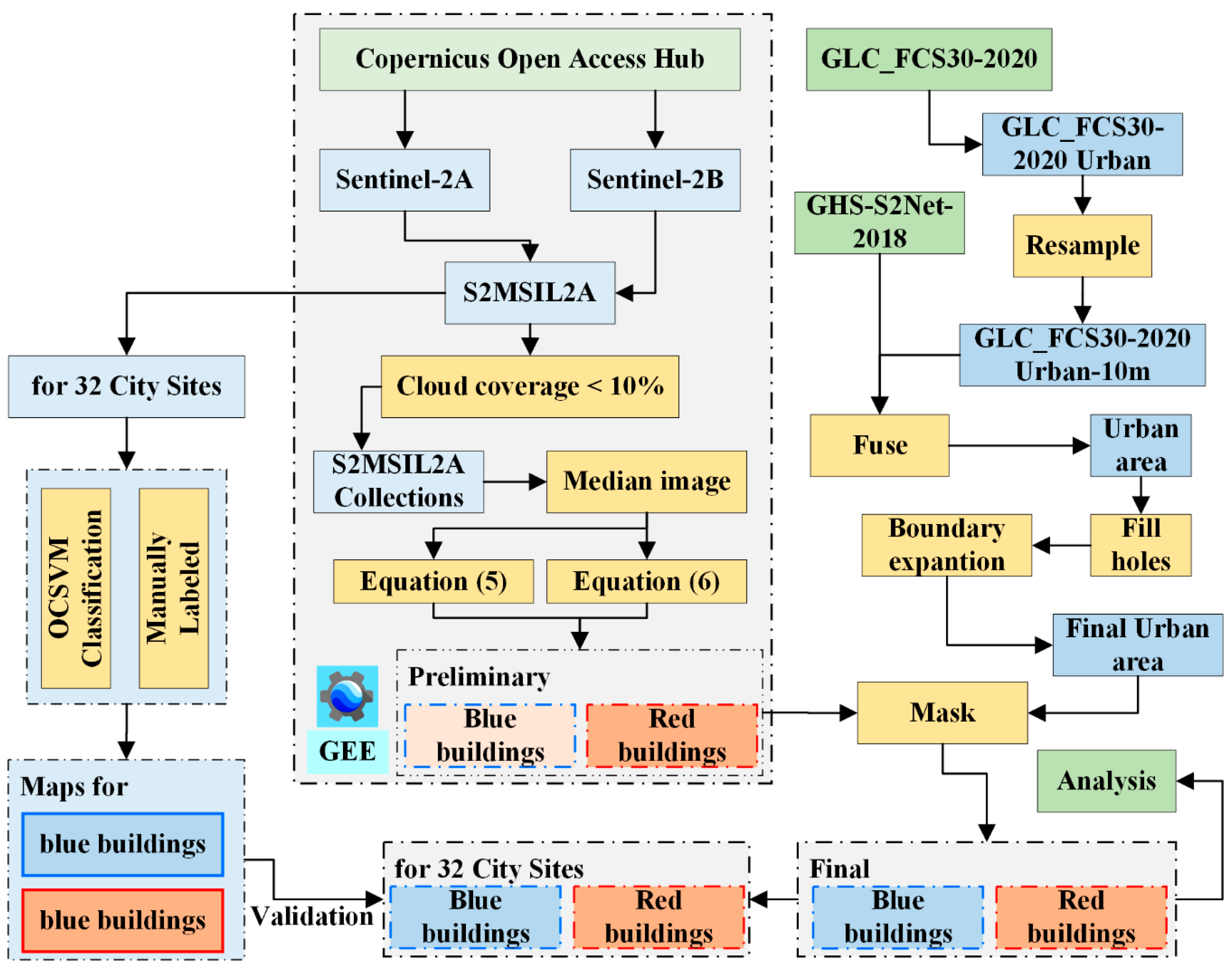
3.4. Blue and Red Building Extraction Method

In the previous Section 3.1, Section 3.2, and Section 3.3, several indexes for blue and red CCSS material extraction have been proposed. To avoid as much as possible limitations due to cloud coverage, only Sentinel 2-A/B MSIL2A images with less than 10% cloud coverage were collected from Copernicus Open Access Hub. Moreover, as mentioned above, to reduce false positives, the GHS-S2Net-2018 map and the urban class from GLC-FCS30-2020 were fused to mask out anything outside the urban areas. The technical steps for blue and red building extraction are presented in Figure 4:

• Step 1: Collect Sentinel-2 A/B S2MSIL2A images with cloud cover ratio lower than 10% that coverage for the whole of China from Copernicus Open Access Hub for 2020;
• Step 2: Obtain the preliminary maps for blue and red CCSS buildings by applying Equations (5) and (6) on the median images of S2MSIL2A image collections;
• Step 3: Produce the urban area map for 2020 by fusion of GHS-S2Net-2018 and GLC-FC30-2020 products;
• Step 4: Obtain the refined maps for blue and red CCSS buildings by masking the preliminary maps produced by step 2 with the urban area map produced by step 3;
• Step 5: Evaluate the performance of the proposed methods on the city sites that selected over different countries with various landscapes;
• Step 6: Analysis for distributions and patterns of blue and red CCSS buildings for China in 2020.

Figure 4. Technical steps for blue and red CCSS buildings extraction.

Figure 4. Technical steps for blue and red CCSS buildings extraction.

3.5. Experimental Setups

To comparatively evaluate and show the performance of the proposed indexes (NDBBI, NDRBI, EBBI, and ERBI), two established indexes, the redness index (RI) and the blueness index (BI), originally developed for soil identification and classification based on soil color Landsat TM data [96], were employed. RI and BI are defined as:

$$\mathrm{RI}=\frac{{\beta }_4}{{\beta }_2+{\beta }_3+{\beta }_4}$$

(7)

$$\mathrm{BI}=\frac{{\beta }_2}{{\beta }_2+{\beta }_3+{\beta }_4}$$

(8)

where ${\beta }_2$, ${\beta }_3,$ and ${\beta }_4$ represent the second (blue), third (green), and fourth (red) Sentinel 2-A/B spectral bands.

Additionally, a one-class support vector machine (OCSVM) classifier, with radial basis function (RBF) kernel from the library for SVM (LIBSVM) toolbox provided by Chang, C.C. and Lin [97] was also used to extract maps to be compared with those by the proposed indexes. For the free parameters of OCSVM, a grid (10 × 10) searching criterion and 3-fold cross-validation technique was adopted by setting the searching range for λ to (0.01–10) and the cost factor range to (1–1000). As evaluation metrics, overall accuracy (OA), Kappa statistic, omission error (OE), and commission error (CE) were selected. All reference maps used in the following experiments were collected by photo-interpretation of RGB (R = band 4, G = band 3, B = band 2) composites of Sentinel 2-A/B images and further referring to the high-resolution optical images in Google Earth.

4. Results and Discussion

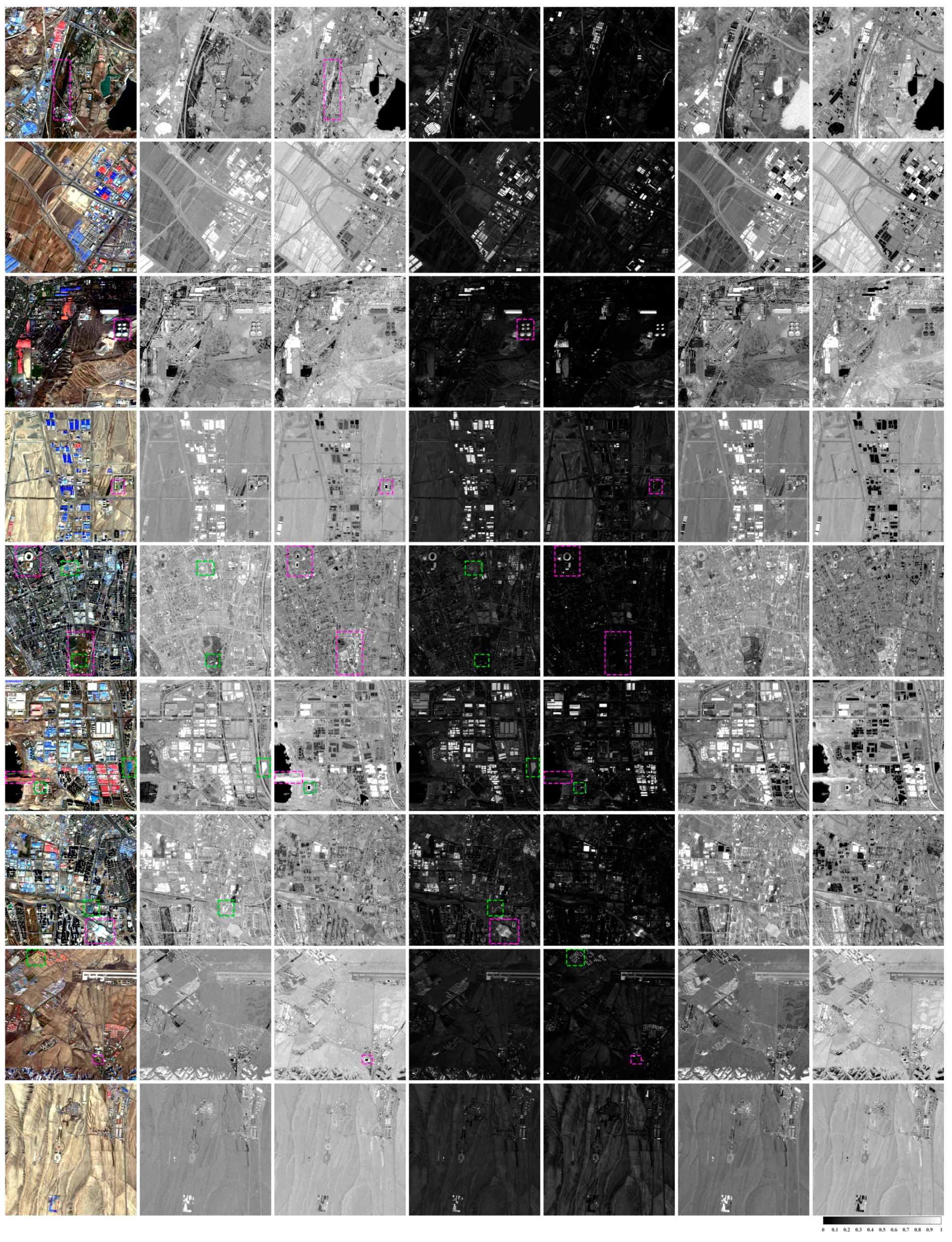
4.1. Visual Evaluation of NDBSI, NDRSI, EBBI, and ERBI Indexes

To show the performance of NDBBI, NDRBI, EBBI, and ERBI indexes for blue and red CCSS roof enhancement, nine distinct sites with different landscape heterogeneity were selected from the Sentinel 2-A image captured on 15 October 2020 over Urumqi. Figure 5 shows the NDBBI, NDRBI, EBBI, and ERBI images for these test sites.

By visually comparing with RGB reference images in the first column and RI and BI images in the sixth and seventh column of Figure 5, most of the blue and red CCSS roof buildings are highlighted by the proposed NDBBI, NDRBI, EBBI, and ERBI. More in detail, while blue CCSS roofs, blue painted asphalt roads as shown by Figure 1b and highlighted with a green rectangle at the bottom of images in the fifth row, construction sites covered by blue nets highlighted with a green rectangle at the right edge of images in the seventh row, snow coverage and hill shadows as shown by the RGB image in the eighth row, are similarly highlighted by NDBBI due to the spectral similarity, and even some water (the Yanerwo lake) is highlighted by BI as shown by the sixth image in firth row, the contrast between blue CCSS roofs and the backgrounds is much higher in the EBBI images in column four. Unfortunately, due to the high and almost flat spectral reflectance at visible spectral bands, some silvery roof buildings and snow patches such as the oil storage tanks highlighted by a pink rectangle in the right images of the third row, the Olympic Center building highlighted by a pink rectangle in the upper-left corner of the images of the fifth row, and the high-speed rail station highlighted by s pink rectangle at the bottom of the images of the seventh row, are also highlighted by EBBI.

In contrast with the results shown by NDRBI and RI images in the third and seventh columns, the improvements by ERBI shown by the images in the fifth column of Figure 5 are clear. For example, NDRBI and IR both enhance red-painted asphalt roads in Yanerwo Park and Liyushan Park, marked by pink rectangles at the bottom center of the images in the first and fifth rows, as well as the plastic racetracks marked by pink rectangles at the middle right of the images in the fourth row, at the upper left of the images in the fifth row, and at the bottom right of the images in the eighth row. They also wrongly enhance rust-colored hill surfaces between two lakes, marked by a pink rectangle at the left edge of the images in the sixth row. Instead, ERBI enhances only the red CCSS roofs, but it has some limitations in distinguishing silver and yellow CCSS roofs, such as in the areas marked by a pink rectangle at the right edge of the images in the third row and by a green rectangle in the upper-left edge of the images in the eighth row of Figure 5.

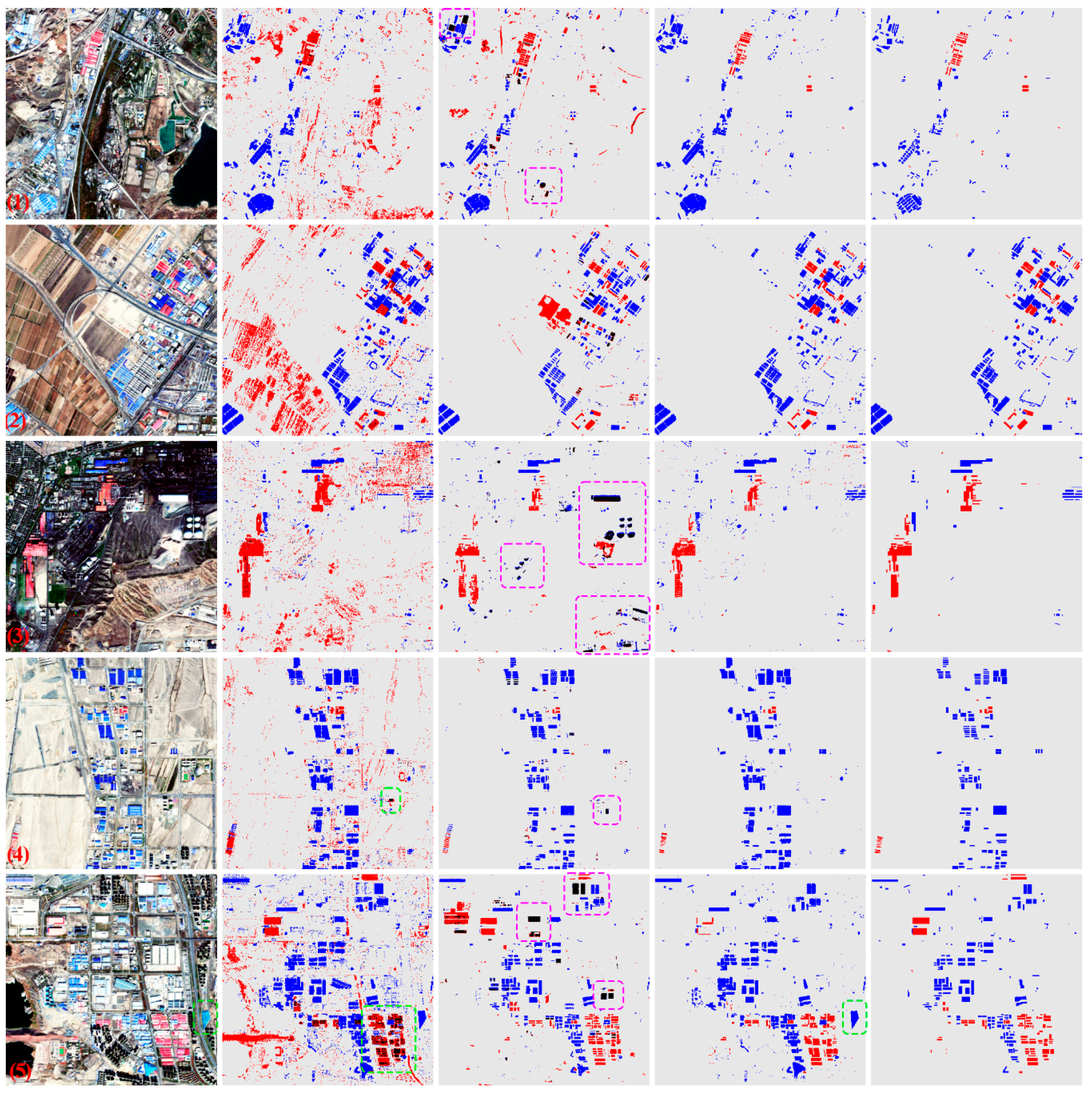
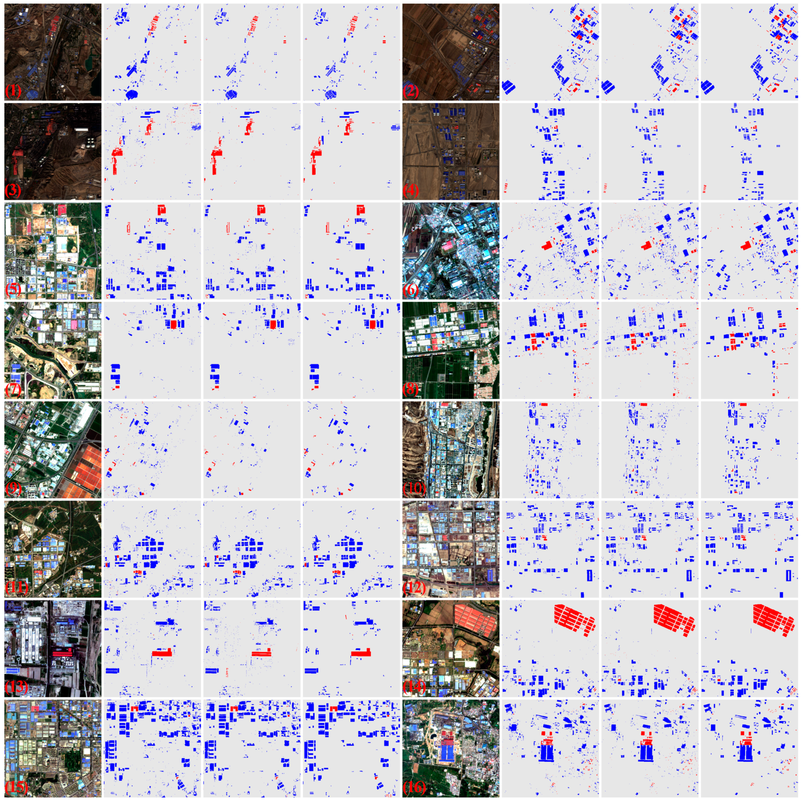
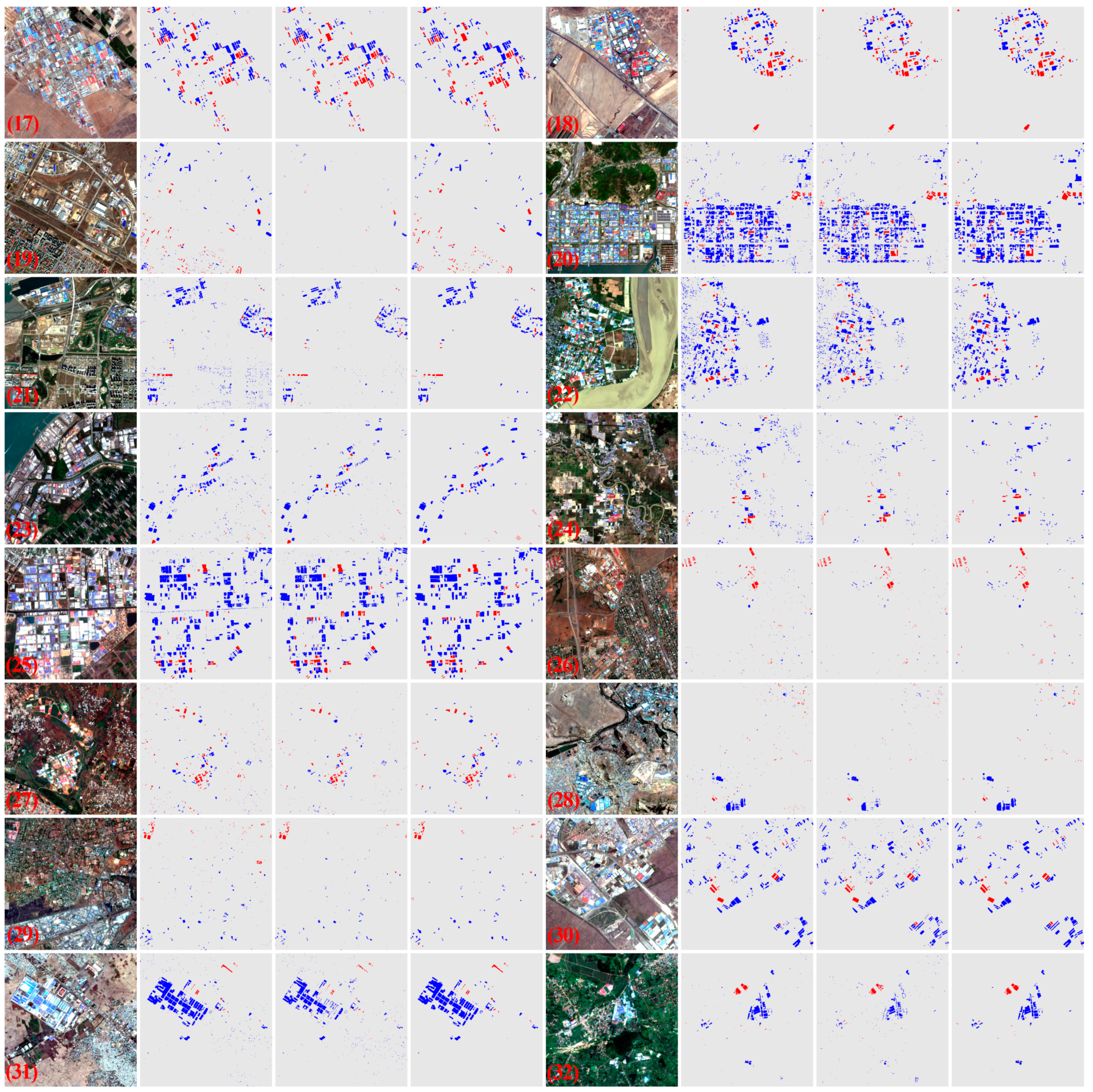
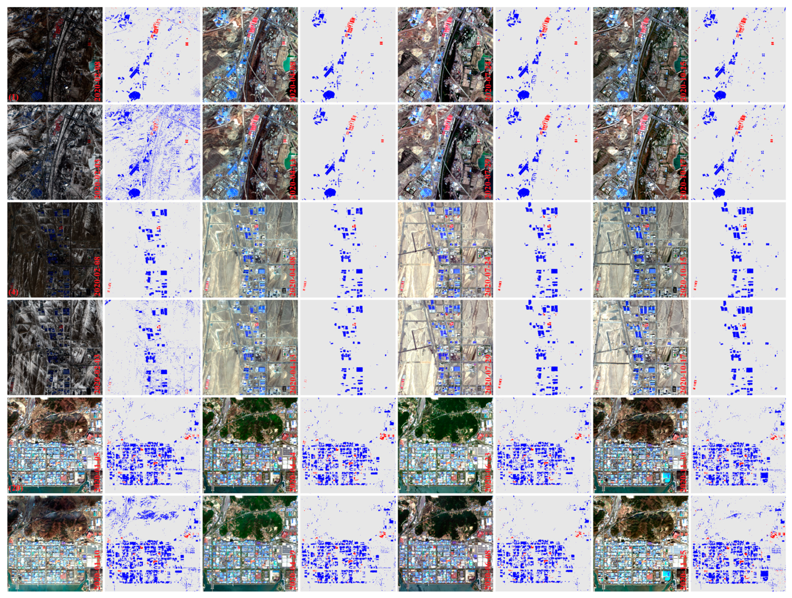
4.2. Results of LBBI and LRBI

To visually and quantitatively compare the performance of NDBBI, NDRBI, EBBI, ERBI, LBBI, and LRBI indexes for blue and red CCSS material roof buildings extraction, five distinct sites with different landscape heterogeneity were selected within the city of Urumqi. The mean-standard deviation plane method [98] was selected to produce binary results from NDBBI, NDRBI, EBBI, and ERBI indexes. Figure 6 shows the detected results for the considered test sites, while

Table 2. Detection accuracy metrics for mean-standard deviation plane method results using NDBBI, NDRBI, EBBI and ERIB, LBBI, and LRBI for 5 sites correspond to Figure 6.

Indexes	NDBBI				NDRBI				EBBI				ERBI				LBBI				LRBI
Evaluation Metrics	OA (%)	Kappa	CE (%)	OE (%)	OA (%)	Kappa	CE (%)	OE (%)	OA (%)	Kappa	CE (%)	OE (%)	OA (%)	Kappa	CE (%)	OE (%)	OA (%)	Kappa	CE (%)	OE (%)	OA (%)	Kappa	CE (%)	OE (%)
1	98.01	0.68	45.70	4.10	94.88	0.16	90.62	0.47	98.22	0.69	42.14	10.48	97.64	0.29	82.54	7.98	98.35	0.72	4.53	40.84	99.80	0.82	14.45	20.60
2	98.52	0.87	21.38	1.14	92.01	0.22	86.39	0.00	97.82	0.76	15.45	28.33	97.60	0.45	67.78	17.73	99.57	0.96	1.06	6.30	99.92	0.97	3.50	3.00
3	98.57	0.56	58.71	11.91	93.89	0.36	76.28	0.07	97.31	0.30	79.04	43.03	97.14	0.45	63.99	35.16	99.19	0.69	11.25	42.94	99.25	0.80	20.69	18.96
4	96.99	0.65	50.42	0.04	96.99	0.65	50.42	0.04	98.71	0.81	29.43	3.29	99.62	0.39	71.61	35.18	98.12	0.75	0.08	38.86	99.94	0.84	14.98	17.14
5	92.88	0.48	66.23	0.67	93.95	0.38	75.26	0.38	97.38	0.70	40.55	11.45	97.23	0.54	59.34	15.42	97.21	0.71	43.23	2.04	98.93	0.71	23.64	32.88
Average	96.99	0.65	48.49	3.57	94.34	0.35	75.79	0.19	97.89	0.65	41.32	19.32	97.85	0.42	69.05	22.29	98.49	0.77	12.03	26.20	99.57	0.83	15.45	18.52
Standard deviation	2.39	0.15	17.07	4.91	1.81	0.19	15.62	0.22	0.59	0.20	23.64	16.13	1.02	0.09	8.80	12.29	0.93	0.11	17.98	20.21	0.45	0.09	7.72	10.65

presents the evaluation metrics.

Based on these results, it is notable that blue and red CCSS roofs can be detected by means of the mean-standard deviation plane method-based segmentation applied to NDBBI and NDRBI, but with a very high false-positive detection rate, particularly from the brown and rust-colored surfaces. For instance, the detection accuracy for NDBBI stays in the range of 92.88–98.57% with an average of 96.99% for OA, in the range of 21.38–66.23% with an average of 48.49% for CE, while the detection accuracy for NDRBI stays in the range of 92.01–96.99% with an average of 94.34% for OA and in the range of 50.42–90.62% with an average of 75.79% for CE, as shown by the numbers in Table 2. The results suing EBBI and ERBI are instead more accurate, but the best results are those by LBBI and LRBI, both visually and quantitatively. For instance, while brown and rust-colored hill surfaces in the first, second, third, and fifth test sites are successfully discarded by the analysis using ERBI, bright buildings such as oil storage tanks and silvery material roof buildings are still detected, as shown by the buildings marked with pink rectangles in the third column of Figure 6. On the contrary, only the blue nest-covered surfaces were detected as blue CCSS material by LBBI index, as marked by the green rectangle in the fourth image of the fifth row in the same figure.

Figure 7 and Figure 8 present blue and red CCSS roof building detection results using LBBI, LRBI, and OCSVM for the sites listed in Table 1, while

Table 3. Detection accuracy metrics for LBBI, LRBI, and OCSVM on considered test sites.

Methods		LBBI				LRBI				OCSVM-BB				OCSVM-RB
Evaluation Metrics		OA (%)	Kappa	CE (%)	OE (%)	OA (%)	Kappa	CE (%)	OE (%)	OA (%)	Kappa	CE (%)	OE (%)	OA (%)	Kappa	CE (%)	OE (%)
Site No.	1	98.35	0.72	4.53	40.84	99.80	0.82	14.45	20.60	99.13	0.80	15.78	22.76	99.86	0.86	8.45	18.61
	2	99.57	0.96	1.06	6.30	99.92	0.97	3.50	3.00	98.99	0.90	8.16	9.95	99.68	0.86	9.52	17.77
	3	99.19	0.69	11.25	42.94	99.25	0.80	20.69	18.96	99.67	0.91	9.40	8.03	99.54	0.74	9.93	37.04
	4	98.12	0.75	0.08	38.86	99.94	0.84	14.98	17.14	99.41	0.90	9.90	10.09	99.94	0.81	8.91	26.71
	5	98.59	0.87	6.19	17.23	99.87	0.93	8.95	4.55	98.57	0.85	7.93	19.17	99.89	0.94	2.45	9.60
	6	99.06	0.91	2.03	13.57	99.92	0.96	2.92	4.86	98.01	0.80	15.23	23.06	99.77	0.89	13.86	8.33
	7	99.65	0.95	1.64	7.95	99.99	0.99	1.43	0.10	99.44	0.92	5.99	10.24	99.95	0.96	4.67	2.49
	8	98.26	0.81	12.07	23.87	99.52	0.83	17.07	17.11	97.94	0.74	19.74	29.59	99.47	0.79	14.00	25.72
	9	99.05	0.76	5.80	35.45	99.87	0.84	16.64	14.41	99.32	0.75	8.43	35.34	99.88	0.84	3.38	25.62
	10	98.15	0.75	22.26	26.17	99.95	0.92	10.84	4.39	98.12	0.72	21.54	32.05	99.96	0.93	1.82	11.86
	11	99.16	0.93	0.71	11.17	99.95	0.93	2.12	11.19	99.11	0.93	6.69	7.30	99.96	0.94	2.89	9.25
	12	98.74	0.90	7.77	10.17	99.96	0.91	11.51	6.10	98.55	0.89	9.89	11.21	99.97	0.92	0.94	13.42
	13	98.84	0.83	7.92	23.66	99.95	0.98	2.85	1.17	98.40	0.72	21.22	31.82	99.71	0.86	7.84	18.80
	14	99.03	0.88	9.72	12.31	98.91	0.90	16.46	0.41	99.51	0.96	3.00	4.66	99.24	0.91	6.43	11.54
	15	97.22	0.88	3.99	16.22	99.89	0.87	22.12	1.36	98.06	0.91	7.88	7.85	99.91	0.89	2.56	18.23
	16	98.25	0.85	6.08	20.43	99.70	0.85	17.14	12.64	98.63	0.87	8.85	15.48	99.77	0.88	9.74	13.02
	17	99.05	0.85	8.96	19.79	99.39	0.84	21.29	8.09	99.16	0.85	12.30	16.11	99.51	0.88	10.30	12.70
	18	99.88	0.96	2.22	4.92	99.91	0.97	3.62	2.17	99.82	0.94	3.98	6.92	99.86	0.95	2.53	6.50
	19	99.64	0.79	4.37	32.66	99.74	0.81	17.57	19.82	99.37	0.28	21.14	83.06	99.35	0.12	17.98	93.39
	20	97.41	0.85	8.06	18.16	99.48	0.76	34.10	10.27	97.28	0.83	11.95	18.80	99.58	0.82	14.95	20.17
	21	98.89	0.77	1.54	35.62	99.97	0.94	4.98	6.60	99.43	0.84	9.29	20.48	99.93	0.86	1.67	23.38
	22	98.97	0.89	1.85	17.67	99.89	0.92	12.13	3.86	98.18	0.78	16.74	25.50	99.85	0.89	6.89	13.94
	23	99.31	0.83	3.28	26.10	99.91	0.82	22.12	14.21	99.46	0.84	11.50	18.78	99.93	0.86	7.73	20.28
	24	99.17	0.69	5.56	45.32	99.93	0.92	8.05	7.29	99.47	0.70	20.08	37.69	99.93	0.92	4.14	11.46
	25	97.95	0.87	6.42	15.87	99.48	0.77	33.70	7.33	97.97	0.87	9.80	14.57	99.66	0.87	14.40	10.31
	26	99.91	0.78	7.38	33.07	99.86	0.88	12.58	10.95	99.84	0.86	10.68	16.02	99.91	0.65	13.50	47.97
	27	99.84	0.88	5.14	18.03	99.75	0.83	3.50	27.42	99.80	0.82	10.71	23.38	99.71	0.73	13.62	36.09
	28	99.82	0.89	9.86	11.58	99.88	0.74	7.80	37.90	99.55	0.66	9.97	48.10	99.91	0.69	11.17	43.39
	29	99.79	0.80	2.47	32.19	99.85	0.80	8.81	27.87	99.83	0.77	11.40	31.20	99.89	0.81	7.48	27.34
	30	99.19	0.87	10.62	15.30	99.85	0.87	19.75	4.84	99.05	0.84	14.23	17.56	99.81	0.84	10.02	21.40
	31	99.44	0.93	4.36	8.04	99.95	0.89	10.47	10.98	98.10	0.73	8.77	37.53	99.86	0.65	28.87	39.83
	32	99.86	0.94	4.41	7.14	99.93	0.89	12.33	8.70	99.25	0.63	21.86	46.02	99.87	0.77	9.87	32.45
Average		98.98	0.85	5.93	21.52	99.79	0.88	13.01	10.82	98.95	0.81	12.00	23.13	99.78	0.82	8.83	22.77
Standard deviation		0.72	0.08	4.43	11.69	0.25	0.07	8.40	8.92	0.70	0.13	5.27	15.93	0.19	0.15	5.86	17.13

shows the detection accuracy metrics, i.e., OA, Kappa, OE, and CE values.

By visually comparing the results shown in Figure 7 for the 16 sites in China and in Figure 8 for another 16 sites in other countries, and looking at the accuracy evaluation values in Table 2, it can be concluded that LBBI and LRBI are highly effective for blue and red CCSS roof building detection. For instance, the detection accuracy for LBBI stays in the range of 97.22–99.88% with an average of 98.98% for OA, in the range of 0.08–22.26% with an average of 5.93% for CE, in the range of 6.30–45.32% with an average of 21.52% for OE. LRBI, instead, reaches detection accuracy with OA values larger than 98.91% with an average of 99.79%, CE values in the range of 1.43–34.10% with an average of 13.01%, OE values in the range of 0.10–37.90% with an average of 10.82% for the 32 selected test sites. The high effectiveness of the proposed LBBI and LRBI can be further checked by comparing the average and standard deviation values with the accuracy assessment values by OCSVM for blue (OCSVM-BB) and red (OCSVM-RB) CCSS roof extraction, shown in the last two rows of Table 3. Considering the detection accuracy values for blue CCSS roofs as an example, both the average (CE = 12.00%, OE = 23.13%) and standard deviation (CE = 5.27%, OE = 15.93%) values for CE and OE by OCSVM-BB are larger than the average (CE = 5.93%, OE = 21.52%) and standard deviation (CE = 4.43%, OE = 11.69%) values for the same quantities using LBBI. Additionally, in comparison with NDBBI, NDRBI, EBBI, and ERBI, LBBI and LRBI are more effective in discriminating blue and red CCSS roofs from silvery CCSS ones, very bright buildings, as well as rust-colored surfaces. For instance, both blue and red CCSS roofs are clearly distinguished from oil storage tanks, rust-colored surfaces, and very bright buildings by LBBI and LRBI for test site (3) in Figure 7 in comparison with the images in the third row of Figure 5, for test site (9) in Figure 7 and for sites (26) and (27) in Figure 8 with respect to the images in the sixth row of Figure 5, and finally for test site (9) in Figure 7 and test site (25) in Figure 8 with respect to the fifth and sixth rows of Figure 5.

It is important to note at this point that, despite they are simple and intuitive, and they have a physical meaning, spectral indexes extracted from satellite data have performances that depend on the sensing conditions, and specifically by the status of the atmosphere, the type of landscape, and the season of acquisition. Still, we expect that LBBI and LRBI indexes are robust enough to cope with these issues. To this aim, detection results for several test sites using Sentinel 2-A and Sentinel 2-B MSIL2A images in different seasons and these indexes are shown in Figure 9. These results show that the worst detection results are always shown by images in the winter season where the land surface is covered by snow (see the images in the first column for sites (1) and (4)) or the vegetated mountain areas, presumably covered by fog (see the first column for site 20). Moreover, the LRBI index for red CCSS roof detection is apparently more robust than the LBBI index for blue CCSS roof detection in different landscapes because, as expected, false positives due to snow and fog mostly appear in the blue CCSS detection results.

According to these results, only Sentinel 2-A/B MSIL2A images collected between April and October are used in the following extraction and the subsequent analyses.

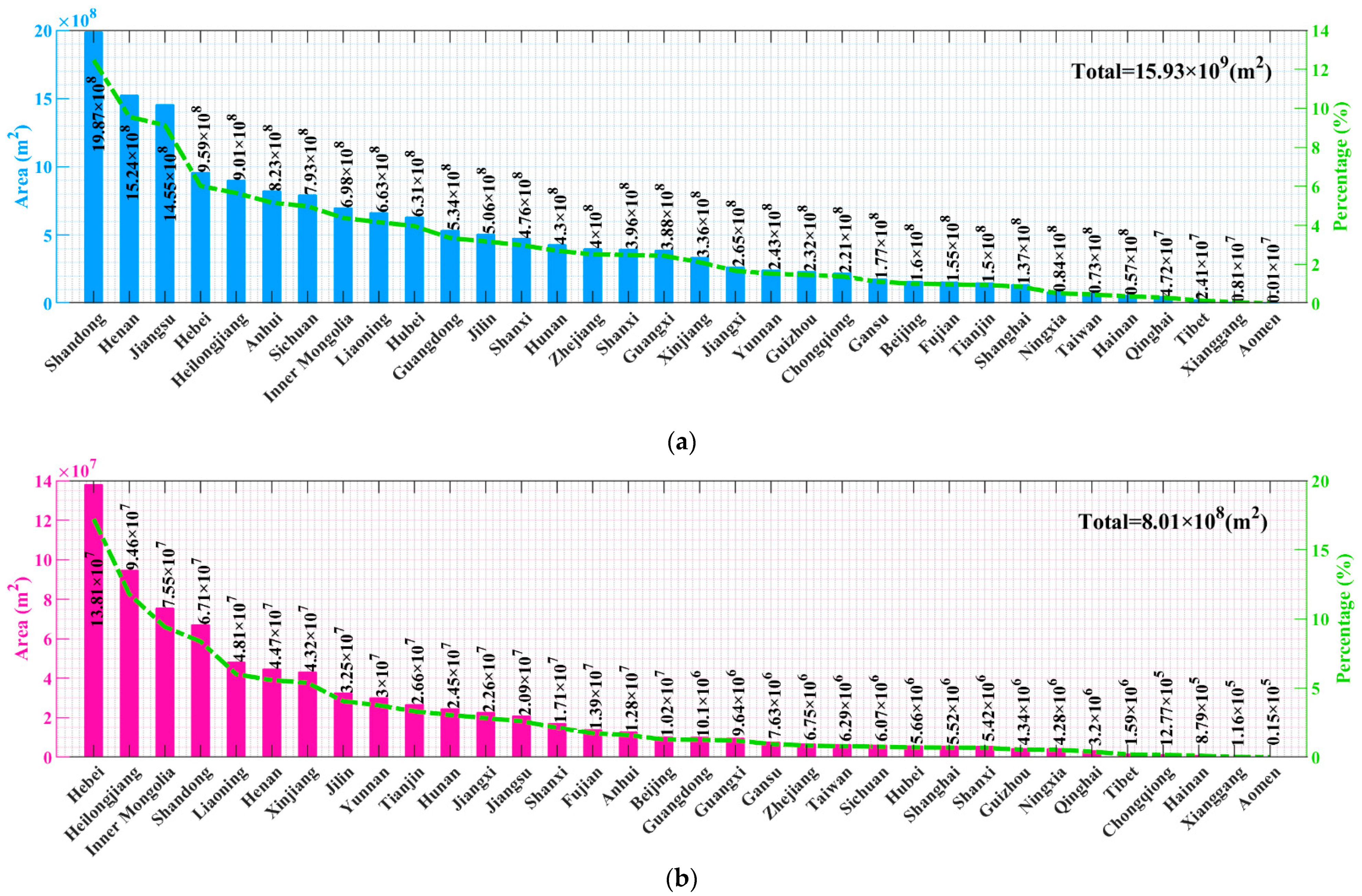
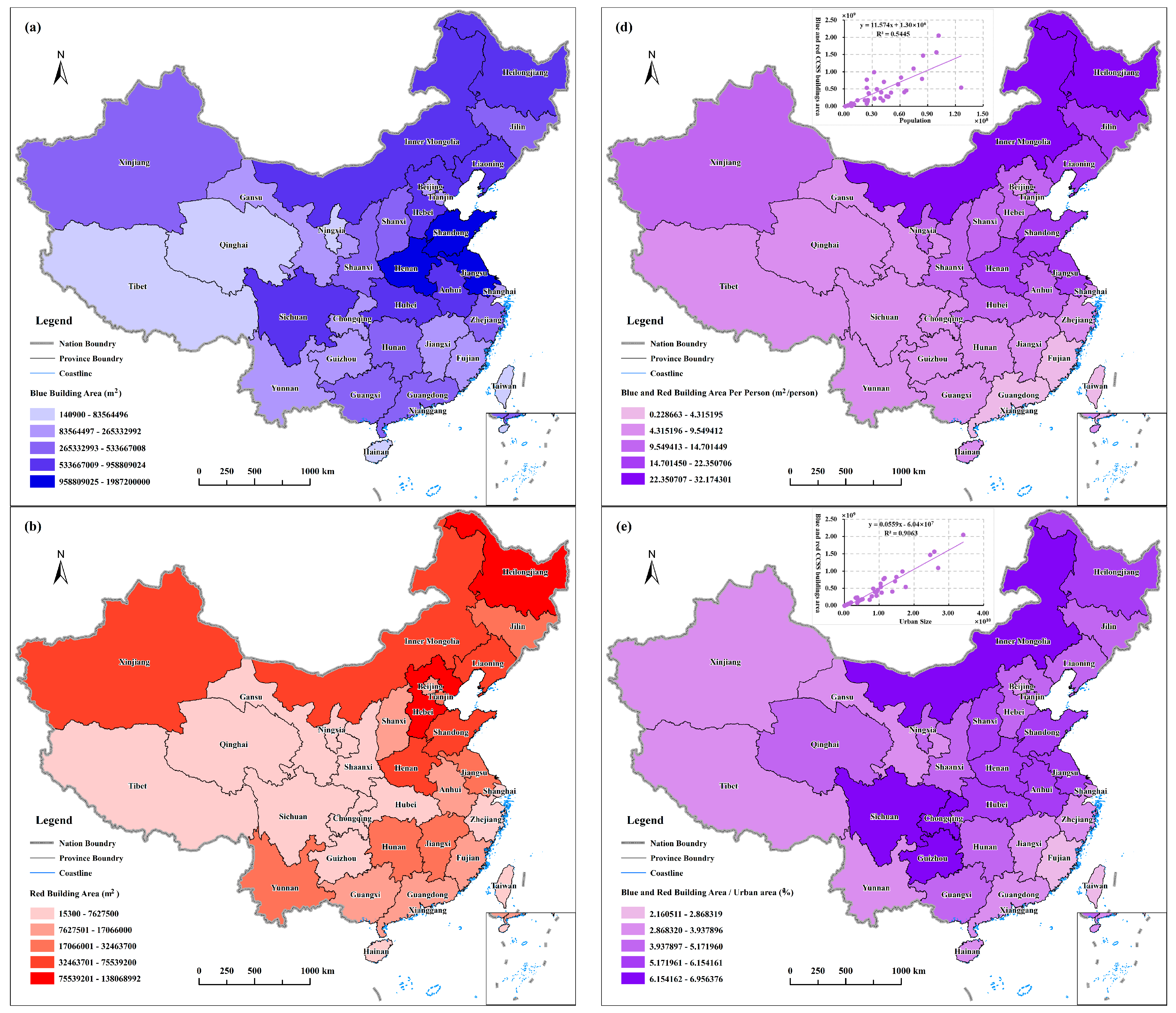
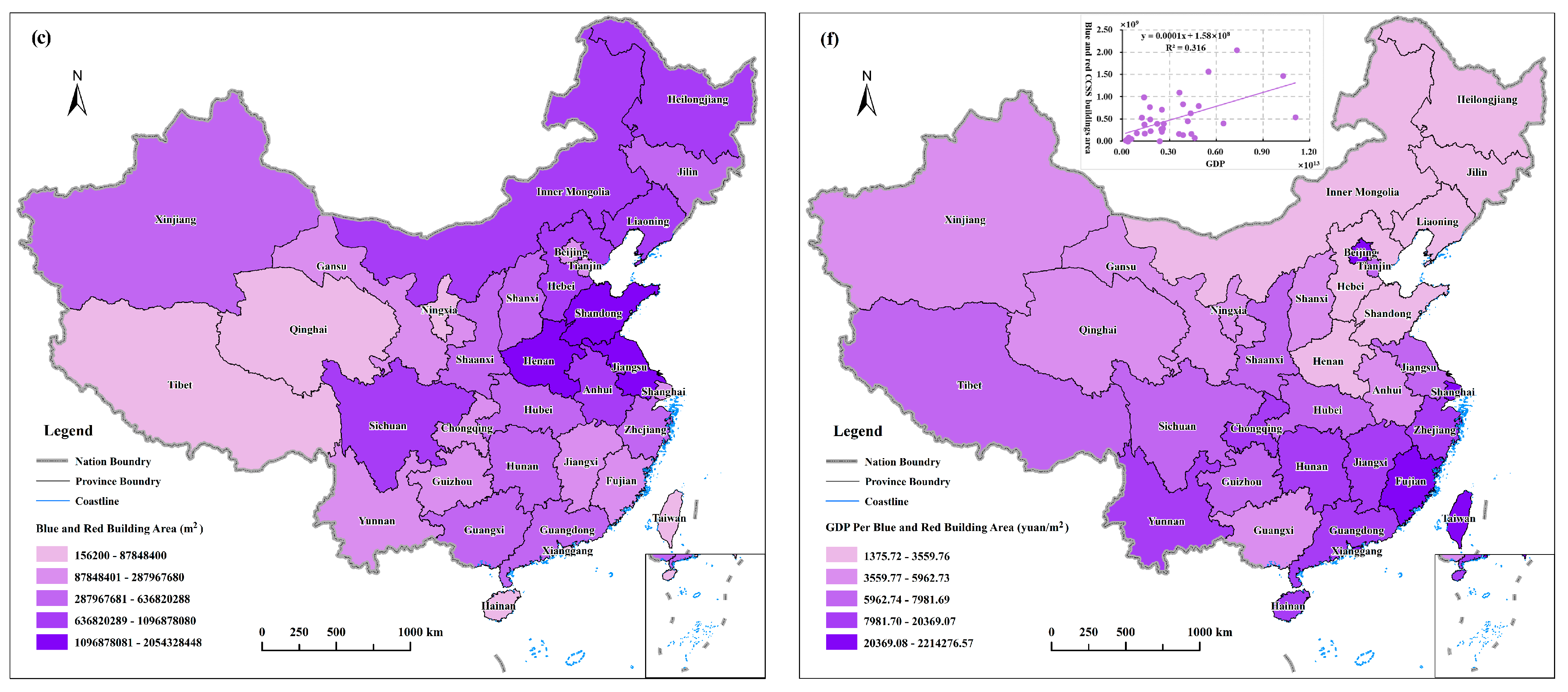
4.3. Distributions and Patterns of Blue and Red CCSS Buildings for China

Exploiting the technique described in Figure 4 and using the logical indexes, blue and red CCSS roofs were extracted for the urban areas across the whole of China. Figure 10 presents bar charts with dashed lines for the area in square meters (m²) and the percentage of blue and red CCSS roof buildings with respect to urban extents at the provincial level in 2020. As mentioned, a large amount of CCSS materials can be usually found on buildings for warehouses, stations, airport terminals, factories, supermarkets, logistic parks, stadiums, and construction sites. Their distribution might thus be connected to socio-economic factors such as population, urbanization, and region development. Hence, in Figure 11, we present maps, colored with five levels, showing the total area of blue and red CCSS roofs and their relation to population (number of inhabitants), urban size (m²), and GDP (RMB) at the provincial level in the same year.

According to the results in Figure 10, the top three areas for blue CCSS roofs are the provinces of Shandong (1.99 × 10⁹ m²), Henan (1.52 × 10⁹ m²), and Jiangsu (1.45 × 10⁹ m²), which account in total for approximately 30% of the blue CCSS covered buildings in China. The top three areas for red CCSS roofs are instead the provinces of Hebei (1.38 × 10⁸ m²), Heilongjiang (9.46 × 10⁸ m²), and Inner Mongolia (7.55 × 10⁹ m²), which together account for approximately 38% of this type of roof in China. By comparing the total areas of blue and red roofs, it can be seen that red roofs are much less common than blue ones. Moreover, in accordance with the results in Figure 10 and Figure 11, blue CCSS roofs are more common in the central and northern provinces, such as Shandong, Henan, Jiangsu, Heilongjiang, Liaoning, and Inner Mongolia, than in the western and southwestern provinces, such as Qinghai, Ningxia, and Xizang. On the contrary, red CCSS roofs are more common in northern provinces. This is because the red CCSS roofs have better thermal capacity than blue roofs; hence, they have a higher use rate in provinces with a colder climate.

As a final analysis, the total area of blue and red CCSS roofs was used to investigate its correlation with a few socio-economic factors. In line with the previous results, and as shown in Figure 11d–f, the northern provinces of Heilongjiang and Inner Mongolia have the highest per capita area of both blue and red CCSS roofs, while the lowest per capita area of these roofs are shown by the southern administrative areas of Guangdong, Hongkong, Fujian, and Taiwan. As for the proportion of the area of blue and red CCSS roofs to the urban extent, the largest ratio (between 6% and 7%) is held by the southwestern provinces of Sichuan, Chongqing, Inner Mongolia, and Guizhou, while the lowest percentage (between 2% and 3%) refers to the Fujian province on the southeast coast. Finally, according to the graded maps shown in Figure 11e, northern provinces such as Henan, Shandong, Hebei, Shanxi, Inner Mongolia, Jilin, and Heilongjiang show the lowest value of GDP per area of blue and red CCSS roofs, while the highest values pertain to Taiwan, Hongkong, Fujian, Shanghai, and Beijing. Further comparing the linear logistic regression charts in the upper-middle parts of Figure 11d–f, we can see that the total area of blue and red CCSS roofs has a weakly significant positive correlation with the population numbers (R2 = 0.5445), a strong correlation with the urban areas’ size (R2 = 0.9063) and a not enough significant correlation with the GDP (R2 = 0.316).

5. Conclusions

In this study, six novel spectral indexes, namely the NDBBI, NDRBI, EBBI, ERBI, LBBI, and LRBI indexes, are proposed for the recognition of blue and red color-coated steel sheet (CCSS) materials. They exploit Sentinel-2A/B MSIL2A data to enhance, detect and extract CCSS roofs in urban areas. NDBBI, NDRBI, EBBI, and ERBI were evaluated in several dense urban area sites by visually comparing them with the existing indexes RI and BI, while LBBI and LRBI were evaluated in 32 urban sites in Asia and Africa by comparing their roof detection results with those by a supervised classification technique, namely OCSVM. Finally, distribution patterns of CCSS roofs, as well as their total, were analyzed area. Relations to a few socio-economic factors at the province level for the whole of China were explored, too. The results demonstrate that NDBBI, NDRBI, EBBI, and ERBI are capable of visually enhancing the blue and red CCSS roofs and that LBBI and LRBI are capable of effectively extracting them.

Moreover, blue and red CCSS roofs are mainly distributed in the northern provinces of China and have an obvious positive correlation with population numbers and the urban area size. Future works will explore how to extend NDBBI, NDRBI, EBBI, ERBI, LBBI, and LRBI for the Landsat 8 operational land imager (OLI) and the Chinese Gaofen and Ziyuan sensors. Additionally, multi-temporal patterns of blue and red CCSS roofs are expected to provide in the future more interesting relations with other socio-economic factors.

References

1. Chen, G.; Li, X.; Liu, X.; Chen, Y.; Liang, X.; Leng, J.; Xu, X.; Liao, W.; Qiu, Y.; Wu, Q.; et al. Global projections of future urban land expansion under shared socioeconomic pathways. Nat. Commun. 2020, 11, 1–12. [Google Scholar] [CrossRef] [Green Version]
2. United Nations. World Urbanization Prospects: The 2018 Revision; United Nations Department of Economic and Social Affairs, Population Division: New York, NY, USA, 2018. [Google Scholar]
3. United Nations. World Population Prospects: The 2017 Revision; United Nations Department of Economic and Social Affairs, Population Division: New York, NY, USA, 2017. [Google Scholar]
4. Zhou, Y.; Li, X.; Asrar, G.R.; Smith, S.J.; Imhoff, M. A global record of annual urban dynamics (1992–2013) from nighttime lights. Remote Sens. Environ. 2018, 219, 206–220. [Google Scholar] [CrossRef]
5. Gong, P.; Li, X.; Wang, J.; Bai, Y.; Chen, B.; Hu, T.; Liu, X.; Xu, B.; Yang, J.; Zhang, W.; et al. Annual maps of global artificial impervious area (GAIA) between 1985 and 2018. Remote Sens. Environ. 2020, 236, 111510. [Google Scholar] [CrossRef]
6. Li, X.; Zhou, Y.; Eom, J.; Yu, S.; Asrar, G.R. Projecting global urban area growth through 2100 based on historical time series data and future Shared Socioeconomic Pathways. Earths Future 2019, 7, 351–362. [Google Scholar] [CrossRef] [Green Version]
7. Govindan, K.; Shankar, K.M.; Kannan, D. Sustainable material selection for construction industry–A hybrid multi criteria decision making approach. Renew. Sustain. Energy Rev. 2016, 55, 1274–1288. [Google Scholar] [CrossRef]
8. Chauvin, J.P.; Glaeser, E.; Ma, Y.; Tobio, K. What is different about urbanization in rich and poor countries? Cities in Brazil, China, India and the United States. J. Urban Econ. 2017, 98, 17–49. [Google Scholar] [CrossRef] [Green Version]
9. Wang, L.; Wang, S.; Zhou, Y.; Liu, W.; Hou, Y.; Zhu, J.; Wang, F. Mapping population density in China between 1990 and 2010 using remote sensing. Remote Sens. Environ. 2018, 210, 269–281. [Google Scholar] [CrossRef]
10. Zhang, W.; Li, W.; Zhang, C.; Hanink, D.M.; Liu, Y.; Zhai, R. Analyzing horizontal and vertical urban expansions in three East Asian megacities with the SS-coMCRF model. Landsc. Urban Plan. 2018, 177, 114–127. [Google Scholar] [CrossRef]
11. Fan, P.; Ouyang, Z.; Nguyen, D.D.; Nguyen, T.T.H.; Park, H.; Chen, J. Urbanization, economic development, environmental and social changes in transitional economies: Vietnam after Doimoi. Landsc. Urban Plan. 2019, 187, 145–155. [Google Scholar] [CrossRef]
12. Grimm, N.B.; Faeth, S.H.; Golubiewski, N.E.; Redman, C.L.; Wu, J.G.; Bai, X.M.; Briggs, J.M. Global change and the ecology of cities. Science 2008, 319, 756–760. [Google Scholar] [CrossRef] [Green Version]
13. Seto, K.C.; Satterthwaite, D. Interactions between urbanization and global environmental change. Curr. Opin. Environ. Sustain. 2010, 2, 127–128. [Google Scholar] [CrossRef]
14. Imhoff, M.L.; Zhang, P.; Wolfe, R.E.; Bounoua, L. Remote sensing of the urban heat island effect across biomes in the continental USA. Remote Sens. Environ. 2010, 114, 504–513. [Google Scholar] [CrossRef] [Green Version]
15. Zhou, D.; Zhao, S.; Zhang, L.; Liu, S. Remotely sensed assessment of urbanization effects on vegetation phenology in China’s 32 major cities. Remote Sens. Environ. 2016, 176, 272–281. [Google Scholar] [CrossRef] [Green Version]
16. He, C.; Gao, B.; Huang, Q.; Ma, Q.; Dou, Y. Environmental degradation in the urban areas of China: Evidence from multi-source remote sensing data. Remote Sens. Environ. 2017, 193, 65–75. [Google Scholar] [CrossRef]
17. Amaya-Espinel, J.D.; Hostetler, M.; Henríquez, C.; Bonacic, C. The influence of building density on Neotropical bird communities found in small urban parks. Landsc. Urban Plan. 2019, 190, 103578. [Google Scholar] [CrossRef]
18. Yu, Z.; Yao, Y.; Yang, G.; Wang, X.; Vejre, H. Strong contribution of rapid urbanization and urban agglomeration development to regional thermal environment dynamics and evolution. For. Ecol. Manag. 2019, 446, 214–225. [Google Scholar] [CrossRef]
19. Wang, Y.; Li, M. Urban Impervious Surface Detection from Remote Sensing Images: A review of the methods and challenges. IEEE Geosci. Remote Sens. Mag. 2019, 7, 64–93. [Google Scholar] [CrossRef]
20. Zhong, Q.; Ma, J.; Zhao, B.; Wang, X.; Zong, J.; Xiao, X. Assessing spatial-temporal dynamics of urban expansion, vegetation greenness and photosynthesis in megacity Shanghai, China during 2000–2016. Remote Sens. Environ. 2019, 233, 111374. [Google Scholar] [CrossRef]
21. Qiu, T.; Song, C.; Zhang, Y.; Liu, H.; Vose, J.M. Urbanization and climate change jointly shift land surface phenology in the northern mid-latitude large cities. Remote Sens. Environ. 2020, 236, 111477. [Google Scholar] [CrossRef]
22. Schneider, A.; Friedl, M.A.; Potere, D. Mapping global urban areas using MODIS 500-m data: New methods and datasets based on ‘urban ecoregions’. Remote Sens. Environ. 2010, 114, 1733–1746. [Google Scholar] [CrossRef]
23. Liu, X.; Hu, G.; Chen, Y.; Li, X.; Xu, X.; Li, S.; Pei, F.; Wang, S. High-resolution multi-temporal mapping of global urban land using Landsat images based on the Google Earth Engine Platform. Remote Sens. Environ. 2018, 209, 227–239. [Google Scholar] [CrossRef]
24. Taubenböck, H.; Roth, A.; Esch, T.; Felbier, A.; Müller, A.; Dech, S. The vision of mapping the global urban footprint using the TerraSAR-X and TanDEM-X mission. In Urban and Regional Data Management; CRC Press: Boca Raton, FL, USA, 2011; pp. 243–251. [Google Scholar]
25. Esch, T.; Heldens, W.; Hirner, A.; Keil, M.; Marconcini, M.; Roth, A.; Zeidler, J.; Dech, S.; Strano, E. Breaking new ground in mapping human settlements from space–The Global Urban Footprint. ISPRS J. Photogramm. Remote Sens. 2017, 134, 30–42. [Google Scholar] [CrossRef] [Green Version]
26. Sharma, R.C.; Tateishi, R.; Hara, K.; Gharechelou, S.; Iizuka, K. Global mapping of urban built-up areas of year 2014 by combining MODIS multispectral data with VIIRS nighttime light data. Int. J. Digit. Earth 2016, 9, 1004–1020. [Google Scholar] [CrossRef]
27. Sinha, P.; Verma, N.K.; Ayele, E. Urban built-up area extraction and change detection of Adama municipal area using time-series Landsat images. Int. J. Adv. Remote Sens. GIS 2016, 5, 1886–1895. [Google Scholar] [CrossRef]
28. Ma, X.; Li, C.; Tong, X.; Liu, S. A New Fusion Approach for Extracting Urban Built-up Areas from Multisource Remotely Sensed Data. Remote Sens. 2019, 11, 2516. [Google Scholar] [CrossRef] [Green Version]
29. Zhang, L.; Weng, Q.; Shao, Z. An evaluation of monthly impervious surface dynamics by fusing Landsat and MODIS time series in the Pearl River Delta, China, from 2000 to 2015. Remote Sens. Environ. 2017, 201, 99–114. [Google Scholar] [CrossRef]
30. Deng, C.; Zhu, Z. Continuous subpixel monitoring of urban impervious surface using Landsat time series. Remote Sens. Environ. 2018, 238, 110929. [Google Scholar] [CrossRef]
31. Shi, K.; Huang, C.; Yu, B.; Yin, B.; Huang, Y.; Wu, J. Evaluation of NPP-VIIRS night-time light composite data for extracting built-up urban areas. Remote Sens. Lett. 2014, 5, 358–366. [Google Scholar] [CrossRef]
32. Che, M.; Gamba, P. Intra-urban change analysis using Sentinel-1 and Nighttime Light Data. IEEE J. Sel. Top. Appl. Earth Obs. Remote Sens. 2019, 12, 1134–1142. [Google Scholar] [CrossRef]
33. Chen, Z.; Yu, B.; Zhou, Y.; Liu, H.; Yang, C.; Shi, K.; Wu, J. Mapping global urban areas from 2000 to 2012 using time-series nighttime light data and MODIS products. IEEE J. Sel. Top. Appl. Earth Obs. Remote Sens. 2019, 12, 1143–1153. [Google Scholar] [CrossRef]
34. Chrysoulakis, N.; Grimmond, S.; Feigenwinter, C.; Lindberg, F.; Gastellu-Etchegorry, J.P.; Marconcini, M.; Mitraka, Z.; Stagakis, S.; Crawford, B.; Olofson, F.; et al. Urban energy exchanges monitoring from space. Sci. Rep. 2018, 8, 1–8. [Google Scholar]
35. Huang, X.; Wang, Y. Investigating the effects of 3D urban morphology on the surface urban heat island effect in urban functional zones by using high-resolution remote sensing data: A case study of Wuhan, Central China. ISPRS J. Photogramm. Remote Sens. 2019, 152, 119–131. [Google Scholar] [CrossRef]
36. Kantakumar, L.N.; Kumar, S.; Schneider, K. SUSM: A scenario-based urban growth simulation model using remote sensing data. Eur. J. Remote Sens. 2019, 52 (Suppl. S2), 26–41. [Google Scholar] [CrossRef] [Green Version]
37. Gao, J.; O’Neill, B.C. Mapping global urban land for the 21st century with data-driven simulations and Shared Socioeconomic Pathways. Nat. Commun. 2020, 11, 1–12. [Google Scholar] [CrossRef]
38. Davidson, F. Planning for performance: Requirements for sustainable development. Habitat Int. 1996, 20, 445–462. [Google Scholar] [CrossRef]
39. Colding, J. ‘Ecological land-use complementation’ for building resilience in urban ecosystems. Landsc. Urban Plan. 2007, 81, 46–55. [Google Scholar] [CrossRef]
40. Van der Linden, S.; Hostert, P. The influence of urban structures on impervious surface maps from airborne hyperspectral data. Remote Sens. Environ. 2009, 113, 2298–2305. [Google Scholar] [CrossRef]
41. Peng, J.; Xie, P.; Liu, Y.; Ma, J. Urban thermal environment dynamics and associated landscape pattern factors: A case study in the Beijing metropolitan region. Remote Sens. Environ. 2016, 173, 145–155. [Google Scholar] [CrossRef]
42. Meng, Q.; Zhang, L.; Sun, Z.; Meng, F.; Wang, L.; Sun, Y. Characterizing spatial and temporal trends of surface urban heat island effect in an urban main built-up area: A 12-year case study in Beijing, China. Remote Sens. Environ. 2018, 204, 826–837. [Google Scholar] [CrossRef]
43. Kobetičová, K.; Černý, R. Terrestrial eutrophication of building materials and buildings: An emerging topic in environmental studies. Sci. Total Environ. 2019, 689, 1316–1328. [Google Scholar] [CrossRef]
44. Kanniyapan, G.; Nesan, L.J.; Mohammad, I.S.; Tan, S.K.; Ponniah, V. Selection criteria of building material for optimising maintainability. Constr. Build. Mater. 2019, 221, 651–660. [Google Scholar] [CrossRef]
45. Cha, G.W.; Moon, H.J.; Kim, Y.C.; Hong, W.H.; Jeon, G.Y.; Yoon, Y.R.; Hwang, C.; Hwang, J.H. Evaluating recycling potential of demolition waste considering building structure types: A study in South Korea. J. Clean. Prod. 2020, 256, 120385. [Google Scholar] [CrossRef]
46. Westermann, P.; Deb, C.; Schlueter, A.; Evins, R. Unsupervised learning of energy signatures to identify the heating system and building type using smart meter data. Appl. Energy 2020, 264, 114715. [Google Scholar] [CrossRef]
47. Mongus, D.; Lukač, N.; Žalik, B. Ground and building extraction from LiDAR data based on differential morphological profiles and locally fitted surfaces. ISPRS J. Photogramm. Remote Sens. 2014, 93, 145–156. [Google Scholar] [CrossRef]
48. Grinias, I.; Panagiotakis, C.; Tziritas, G. MRF-based segmentation and unsupervised classification for building and road detection in peri-urban areas of high-resolution satellite images. ISPRS J. Photogramm. Remote Sens. 2016, 122, 145–166. [Google Scholar] [CrossRef]
49. Du, S.; Luo, L.; Cao, K.; Shu, M. Extracting building patterns with multilevel graph partition and building grouping. ISPRS J. Photogramm. Remote Sens. 2016, 122, 81–96. [Google Scholar] [CrossRef]
50. He, X.; Zhang, X.; Xin, Q. Recognition of building group patterns in topographic maps based on graph partitioning and random forest. ISPRS J. Photogramm. Remote Sens. 2018, 136, 26–40. [Google Scholar] [CrossRef]
51. Huang, J.; Zhang, X.; Xin, Q.; Sun, Y.; Zhang, P. Automatic building extraction from high-resolution aerial images and LiDAR data using gated residual refinement network. ISPRS J. Photogramm. Remote Sens. 2019, 151, 91–105. [Google Scholar] [CrossRef]
52. Shi, Y.; Li, Q.; Zhu, X.X. Building segmentation through a gated graph convolutional neural network with deep structured feature embedding. ISPRS J. Photogramm. Remote Sens. 2020, 159, 184–197. [Google Scholar] [CrossRef]
53. Rodríguez-Álvarez, J. Urban Energy Index for Buildings (UEIB): A new method to evaluate the effect of urban form on buildings’ energy demand. Landsc. Urban Plan. 2016, 148, 170–187. [Google Scholar] [CrossRef]
54. Custódio, J.V.; Agostinho, S.M.; Simões, A.M. Electrochemistry and surface analysis of the effect of benzotriazole on the cut edge corrosion of galvanized steel. Electrochim. Acta 2010, 55, 5523–5531. [Google Scholar] [CrossRef]
55. Hernández-Pérez, I.; Zavala-Guillén, I.; Xamán, J.; Belman-Flores, J.M.; Macias-Melo, E.V.; Aguilar-Castro, K.M. Test box experiment to assess the impact of waterproofing materials on the energy gain of building roofs in Mexico. Energy 2019, 186, 115847. [Google Scholar] [CrossRef]
56. Torres-Quezada, J.; Coch, H.; Isalgué, A. Assessment of the reflectivity and emissivity impact on light metal roofs thermal behaviour, in warm and humid climate. Energy Build. 2019, 188, 200–208. [Google Scholar] [CrossRef]
57. Hu, J.; Chen, W.; Qu, Y.; Yang, D. Safety and serviceability of membrane buildings: A critical review on architectural, material and structural performance. Eng. Struct. 2020, 210, 110292. [Google Scholar] [CrossRef]
58. Lee, C.Y.; Kaneko, S.; Sharifi, A. Effects of building types and materials on household electricity consumption in Indonesia. Sustain. Cities Soc. 2020, 54, 101999. [Google Scholar] [CrossRef]
59. Xamán, J.; Rodriguez-Ake, A.; Zavala-Guillén, I.; Hernández-Pérez, I.; Arce, J.; Sauceda, D. Thermal performance analysis of a roof with a PCM-layer under Mexican weather conditions. Renew. Energy 2020, 149, 773–785. [Google Scholar] [CrossRef]
60. Xie, S.; Ji, Z.; Zhu, L.; Zhang, J.; Cao, Y.; Chen, J.; Liu, R.; Wang, J. Recent progress in electromagnetic wave absorption building materials. J. Build. Eng. 2020, 27, 100963. [Google Scholar] [CrossRef]
61. Heiden, U.; Segl, K.; Roessner, S.; Kaufmann, H. Determination of robust spectral features for identification of urban surface materials in hyperspectral remote sensing data. Remote Sens. Environ. 2007, 111, 537–552. [Google Scholar] [CrossRef] [Green Version]
62. Chisense, C.; Hahn, M.; Engels, J. Classification of roof materials using hyperspectral data. International Archives of the Photogrammetry. Remote Sens. Spat. Inf. Sci. 2012, 39, 103. [Google Scholar]
63. Yuan, L.; Guo, J.; Wang, Q. Automatic classification of common building materials from 3D terrestrial laser scan data. Autom. Constr. 2020, 110, 103017. [Google Scholar] [CrossRef]
64. Guo, X.; Li, P. Mapping plastic materials in an urban area: Development of the normalized difference plastic index using WorldView-3 superspectral data. ISPRS J. Photogramm. Remote Sens. 2020, 169, 214–216. [Google Scholar] [CrossRef]
65. Wang, J.; Yang, W.; Yang, S.; Yan, H. Spatial Distribution Characteristics of Color Steel Plate Buildings in Lanzhou City; Modern Environmental Science and Engineering: Brooklyn, NY, USA, 2019; p. 583. [Google Scholar]
66. Wang, J.; Yang, W.; Yang, S.; Ma, J. Research on spatial distribution characteristics of color steel buildings in Anniing district of Lanzhou. J. Lanzhou Jiaotong Univ. 2019, 38, 110–114. [Google Scholar]
67. Yu, B.; Liu, H.; Wu, J.; Hu, Y.; Zhang, L. Automated derivation of urban building density information using airborne LiDAR data and object-based method. Landsc. Urban Plan. 2010, 98, 210–219. [Google Scholar] [CrossRef]
68. Zhang, T.; Huang, X.; Wen, D.; Li, J. Urban building density estimation from high-resolution imagery using multiple features and support vector regression. IEEE J. Sel. Top. Appl. Earth Obs. Remote Sens. 2017, 10, 3265–3280. [Google Scholar] [CrossRef]
69. Maltezos, E.; Doulamis, A.; Doulamis, N.; Ioannidis, C. Building extraction from LiDAR data applying deep convolutional neural networks. IEEE Geosci. Remote Sens. Lett. 2018, 16, 155–159. [Google Scholar] [CrossRef]
70. Brunner, D.; Lemoine, G.; Bruzzone, L.; Greidanus, H. Building height retrieval from VHR SAR imagery based on an iterative simulation and matching technique. IEEE Trans. Geosci. Remote Sens. 2009, 48, 1487–1504. [Google Scholar] [CrossRef]
71. Nie, X.; Qiao, H.; Zhang, B. A variational model for PolSAR data speckle reduction based on the Wishart distribution. IEEE Trans. Image Processing 2015, 24, 1209–1222. [Google Scholar]
72. Zheng, J.; Zeng, C.; Zhang, H. Scattering Modeling of Urban Oriented Buildings in PolSAR images by Using Adaptive Statistical Distribution. IEEE Access 2019, 7, 147119–147128. [Google Scholar] [CrossRef]
73. Gorelick, N.; Hancher, M.; Dixon, M.; Ilyushchenko, S.; Thau, D.; Moore, R. Google Earth Engine: Planetary-scale geospatial analysis for everyone. Remote Sens. Environ. 2017, 202, 18–27. [Google Scholar] [CrossRef]
74. Kumar, L.; Mutanga, O. Google Earth Engine applications since inception: Usage, trends, and potential. Remote Sens. 2018, 10, 1509. [Google Scholar] [CrossRef] [Green Version]
75. Tamiminia, H.; Salehi, B.; Mahdianpari, M.; Quackenbush, L.; Adeli, S.; Brisco, B. Google Earth Engine for geo-big data applications: A meta-analysis and systematic review. ISPRS J. Photogramm. Remote Sens. 2020, 164, 152–170. [Google Scholar] [CrossRef]
76. Amani, M.; Ghorbanian, A.; Ahmadi, S.A.; Kakooei, M.; Moghimi, A.; Mirmazloumi, S.M.; Moghaddam, S.H.A.; Mahdavi, S.; Ghahremanloo, M.; Parsian, S.; et al. Google earth engine cloud computing platform for remote sensing big data applications: A comprehensive review. IEEE J. Sel. Top. Appl. Earth Obs. Remote Sens. 2020, 13, 5326–5350. [Google Scholar] [CrossRef]
77. Wang, L.; Diao, C.; Xian, G.; Yin, D.; Lu, Y.; Zou, S.; Erickson, T.A. A summary of the special issue on remote sensing of land change science with Google earth engine. Remote Sens. Environ. 2020, 248, 112002. [Google Scholar] [CrossRef]
78. Wang, W.; Samat, A.; Ge, Y.; Ma, L.; Tuheti, A.; Zou, S.; Abuduwaili, J. Quantitative soil wind erosion potential mapping for Central Asia using the Google Earth Engine platform. Remote Sens. 2020, 12, 3430. [Google Scholar] [CrossRef]
79. Zhao, Q.; Yu, L.; Li, X.; Peng, D.; Zhang, Y.; Gong, P. Progress and Trends in the Application of Google Earth and Google Earth Engine. Remote Sens. 2021, 13, 3778. [Google Scholar] [CrossRef]
80. Fan, S.; Sun, C. Production Technology for Colour Coated Steel Sheet. Angang Technol. 2004, 4, 1. [Google Scholar]
81. Annual Research and Consultation Report of Panorama Survey and Investment Strategy on China Strategy. Available online: https://www.chinairn.com/report/20210526.html (accessed on 25 April 2021).
82. Ma, J.; Yang, S.; Jia, X.; Yan, R. Temporal and spatial change of color steel sheds in Anning district of Lanzhou city. Sci. Surv. Mapp. 2018, 43, 34–37. [Google Scholar]
83. Wang, S.; Ju, W.; Peñuelas, J.; Cescatti, A.; Zhou, Y.; Fu, Y.; Huete, A.; Liu, M.; Zhang, Y. Urban− rural gradients reveal joint control of elevated CO2 and temperature on extended photosynthetic seasons. Nat. Ecol. Evol. 2019, 3, 1076–1085. [Google Scholar] [CrossRef] [Green Version]
84. Chen, Z.S.; Martínez, L.; Chang, J.P.; Wang, X.J.; Xionge, S.H.; Chin, K.S. Sustainable building material selection: A QFD-and ELECTRE III-embedded hybrid MCGDM approach with consensus building. Eng. Appl. Artif. Intell. 2019, 85, 783–807. [Google Scholar] [CrossRef]
85. Martin Schaefer, H.; Schaefer, V.; Vorobyev, M. Are fruit colors adapted to consumer vision and birds equally efficient in detecting colorful signals? Am. Nat. 2007, 169, S159–S169. [Google Scholar] [CrossRef]
86. Robb, M.J.; Ku, S.Y.; Brunetti, F.G.; Hawker, C.J. A renaissance of color: New structures and building blocks for organic electronics. J. Polym. Sci. Part A Polym. Chem. 2013, 51, 1263–1271. [Google Scholar] [CrossRef]
87. Ren, J.; Liang, H.; Chan, F.T. Urban sewage sludge, sustainability, and transition for Eco-City: Multi-criteria sustainability assessment of technologies based on best-worst method. Technol. Forecast. Soc. Change 2017, 116, 29–39. [Google Scholar] [CrossRef]
88. Leveau, L.M. Urbanization induces bird color homogenization. Landsc. Urban Plan. 2019, 192, 103645. [Google Scholar] [CrossRef]
89. Li, P.; Yang, S.; Yao, H.; Yang, M.; Yong, W. Research on Extraction of the Urban Color Steel Shed Based on High-resolution Remote Sensing Images. Geospat. Inf. 2017, 15, 13–18. [Google Scholar]
90. Ye, C.M.; Cui, P.; Pirasteh, S.; Li, J.; Li, Y. Experimental approach for identifying building surface materials based on hyperspectral remote sensing imagery. J. Zhejiang Univ.-Sci. A 2017, 18, 984–990. [Google Scholar] [CrossRef]
91. Drusch, M.; Del Bello, U.; Carlier, S.; Colin, O.; Fernandez, V.; Gascon, F.; Hoersch, B.; Isola, C.; Laberinti, P.; Martimort, P.; et al. Sentinel-2: ESA’s optical high-resolution mission for GMES operational services. Remote Sens. Environ. 2012, 120, 25–36. [Google Scholar] [CrossRef]
92. Zhang, X.; Liu, L.; Chen, X.; Gao, Y.; Xie, S.; Mi, J. GLC_FCS30: Global land-cover product with fine classification system at 30 m using time-series Landsat imagery. Earth Syst. Sci. Data 2021, 13, 2753–2776. [Google Scholar] [CrossRef]
93. Corbane, C.; Syrris, V.; Sabo, F.; Politis, P.; Melchiorri, M.; Pesaresi, M.; Soille, P.; Kemper, T. Convolutional neural networks for global human settlements mapping from Sentinel-2 satellite imagery. Neural Comput. Appl. 2021, 33, 6697–6720. [Google Scholar] [CrossRef]
94. Chen, J.; Jönsson, P.; Tamura, M.; Gu, Z.; Matsushita, B.; Eklundh, L. A simple method for reconstructing a high-quality NDVI time-series data set based on the Savitzky–Golay filter. Remote Sens. Environ. 2004, 91, 332–344. [Google Scholar] [CrossRef]
95. Babaei, H.; Janalipour, M.; Tehrani, N.A. A simple, robust, and automatic approach to extract water body from Landsat images (case study: Lake Urmia, Iran). J. Water Clim. Change 2021, 12, 238–249. [Google Scholar] [CrossRef] [Green Version]
96. Escadafal, R. Remote sensing of soil color: Principles and applications. Remote Sens. Rev. 1993, 7, 261–279. [Google Scholar] [CrossRef]
97. Chang, C.C.; Lin, C.J. LIBSVM: A library for support vector machines. ACM Trans. Intell. Syst. Technol. (TIST) 2011, 2, 1–27. [Google Scholar] [CrossRef]
98. Maussang, F.; Chanussot, J.; Hetet, A. Automated segmentation of SAS images using the mean-standard deviation plane for the detection of underwater mines. In Proceedings of the Oceans 2003. Celebrating the Past ... Teaming Toward the Future (IEEE Cat. No.03CH37492), San Diego, CA, USA, 22–26 September 2003; Volume 4, pp. 2155–2160. [Google Scholar]
Figure 1. WorldView-3 RGB image captured on 22 July 2020 and ground photos of blue and red materials (aj) around Liyushan Park at Urumqi City, Xinjiang, China.
Remotesensing 14 00230 g001
Figure 2. Study area and the distribution of the cities used as test sites over China.
Remotesensing 14 00230 g002
Figure 3. Sentinel 2-A MSIL2A average image spectra of CCSS materials and other land cover types collected from upper half (a) and lower half (b) parts of Figure 1.
Remotesensing 14 00230 g003
Figure 5. RGB images (column 1), NDBBI (column 2), NDRBI (column 3), EBBI (column 4), ERBI (column 5), BI (column 6) and RI (column 7) for total 9 test sites from Urumqi City. (Red numbers at the lower-left corner of RGB images represent the row number).
Remotesensing 14 00230 g005
Figure 6. RGB images (column 1), mean-standard deviation plane method results using NDBBI-NDRBI (column 2), EBBI-ERBI (column 3), LBBI-LRBI (column 4), to be compared with the ground truth (column 5) for 5 test sites in the city of Urumqi (row numbers are included in red at the lower-left corner of the RGB images for an easier reference in the text).
Remotesensing 14 00230 g006
Figure 7. RGB images (columns 1, 5), detected results from LBBI and LRBI (column 2, 6), OCSVM (column 3, 7), and ground truths (column 4, 8) for 16 test sites from China (red numbers at the lower-left corner correspond to site numbers in Table 1, blue and red colors represent the detected blue and red buildings, respectively).
Remotesensing 14 00230 g007
Figure 8. RGB images (columns 1, 5), detected results using LBBI and LRBI (columns 2, 6), OCSVM (columns 3, 7), and ground truths (columns 4, 8) for 16 test sites from Asia and Africa (red numbers at the lower-left corner correspond to the site number in Table 1, blue and red colors represent the detected blue and red buildings, respectively).
Remotesensing 14 00230 g008
Figure 9. RGB images (columns 1, 3, 5 and 7) and detected results by LBBI and LRBI (columns 2, 4, 6 and 8) using Sentinel-2A (rows 1, 3 and 5) and Sentinel-2B (rows 2, 4 and 6) on four seasons (red numbers at the lower-left corner correspond to site numbers in Table 1, red numbers at the lower right corner represent the sensing day).
Remotesensing 14 00230 g009
Figure 10. Area in square meters (m2) and proportion in percentage of blue (a) and red (b) CCSS roof buildings for provincial-level administrative areas of China in 2020.
Remotesensing 14 00230 g010
Figure 11. Graded maps for areas of blue (a), red (b), and blue plus red (c) CCSS roof buildings and their relations to population (d), urban size (e), and GDP (f) for provincial-level administrative areas of China in 2020.
Remotesensing 14 00230 g011aRemotesensing 14 00230 g011b