Article

Target Classification of Similar Spatial Characteristics in Complex Urban Areas by Using Multispectral LiDAR

1
School of Geography and Information Engineering, China University of Geosciences, Wuhan 430074, China
2
Artificial Intelligence School, Wuchang University of Technology, Wuhan 430223, China
3
State Key Laboratory of Magnetic Resonance and Atomic and Molecular Physics, Innovation Academy for Precision Measurement Science and Technology, Chinese Academy of Sciences, Wuhan 430071, China
4
State Key Laboratory of Information Engineering in Surveying, Mapping and Remote Sensing, Wuhan University, 129 Luoyu Road, Wuhan 430072, China
5
Electronic Information School, Wuhan University, Wuhan 430072, China
*
Author to whom correspondence should be addressed.
Submission received: 4 November 2021 / Revised: 8 December 2021 / Accepted: 1 January 2022 / Published: 5 January 2022
(This article belongs to the Special Issue Land Cover Classification Using Multispectral LiDAR Data)

Abstract

:
With the rapid modernization, many remote-sensing sensors were developed for classifying urban land and environmental monitoring. Multispectral LiDAR, which serves as a new technology, has exhibited potential in remote-sensing monitoring due to the synchronous acquisition of three-dimension point cloud and spectral information. This study confirmed the potential of multispectral LiDAR for complex urban land cover classification through three comparative methods. Firstly, the Optech Titan LiDAR point cloud was pre-processed and ground filtered. Then, three methods were analyzed: (1) Channel 1, based on Titan data to simulate the classification of a single-band LiDAR; (2) three-channel information and the digital surface model (DSM); and (3) three-channel information and DSM combined with the calculated three normalized difference vegetation indices (NDVIs) for urban land classification. A decision tree was subsequently used in classification based on the combination of intensity information, elevation information, and spectral information. The overall classification accuracies of the point cloud using the single-channel classification and the multispectral LiDAR were 64.66% and 93.82%, respectively. The results show that multispectral LiDAR has excellent potential for classifying land use in complex urban areas due to the availability of spectral information and that the addition of elevation information to the classification process could boost classification accuracy.

1. Introduction

Urban land use classification is an essential component of land planning and national monitoring. Remote sensing has the characteristics of timeliness, periodicity, and a wide range, which makes it an essential tool for classifying urban land use types. In general, hyperspectral resolution images are utilized in land-use classification. Although the results are satisfactory [1,2], the lack of three-dimensional (3D) information in hyperspectral images makes 3D urban land use classification difficult. Consequently, the 3D point cloud-based LiDAR classification method is widely used in urban land-use classification due to its high accuracy and convenience advantages. Similar to the development of passive optical remote sensing, the development of LiDAR has also gone through a single wavelength–multispectral–hyperspectral development phase [3]. Among them, multispectral LiDAR is the most widely used and shows excellent potential for the application of complex urban land monitoring. Compared to single-band LiDAR for urban land-use classification, Multispectral LiDAR systems can acquire high-density multispectral point clouds by emitting laser pulses of different wavelengths. It has become a commonly used source of data for 3D land-use classification [4]. Airborne LiDAR is an aircraft-mounted laser detection and ranging system that measures the 3D coordinates of objects on the ground [5]. LiDAR offers easy access to high-resolution data; therefore, it is widely used in resource exploration [6,7,8], urban planning [9,10], agricultural development [11,12], land use [13,14], and environmental monitoring [15,16,17,18], etc. LiDAR land-use classification methods can be divided into two-dimensional (2D) based image classifications and 3D point cloud classifications. The 2D image-based methods tend to take the intensity information and echo information from the LiDAR and to rasterize them into a 2D image for classification. This method is often suitable for using in large-scale land-use classification. Li et al. [19] proposed an object-oriented land-cover classification method based on SVM with multiple data fusion, which uses aerial images and LiDAR data to link the raster and vector analysis domains. The LiDAR-derived digital surface model (DSM) information can be obtained with higher accuracy. In particular, object-oriented SVM classification has been shown to be correct in effectively identifying various shadows. Wang et al. [20] used an object-oriented classification approach, using multispectral images as the primary data source and LiDAR DSM as auxiliary data for urban land-use classification. With an overall accuracy of 90.7%, the study pointed out that the combination of LiDAR height and intensity data could accurately map urban land cover. This 2D image-based method is usually accurate and less costly for image classification. However, this method is more expensive for large areas of LiDAR and loses accuracy when the data is downscaled [21]. The 3D spatially based classification is similar to pixel-based classification for individual 3D point clouds; this method refines the spatial information. Dai et al. [22] used a mean drift segmentation method to classify tree species in different feature spaces. Ten sample plots from a dense coniferous forest area in Tobermory, Ontario, Canada, were selected as experimental data. The results demonstrated that the accuracy is 88% and 82% with and without multispectral information, respectively. Compared to segmentation using geometric spatial information alone, clustered tree segmentation has significant multispectral characteristics. Ekhtari et al. [23] used the Titan multispectral LiDAR dataset to classify point clouds into ten different land-cover classes by using the laser return intensity and a spatial metric calculated from the 3D position of the laser returns. A rule-based classifier was used to classify the multiple return points with an overall accuracy of 79.7%. The results showed that this algorithm outperforms the usual point cloud rasterization method. However, this 3D point cloud-based classification comes at the cost of increased complexity and computational burden.
Initially, for airborne LiDAR classification, many classification methods are based on the single-band intensity data combined with digital surface model (DSM) [24,25]. Charaniya et al. [26] used the Gaussian mixture model algorithm for classification. LiDAR data combined with DSM data were classified into roads, grass, buildings, and trees. However, there existed outliers in the classification due to the LiDAR receiver noise. Thus, the accuracy of classification ranged from 66% to 84%. Lodha et al. [27] used the support vector machine (SVM) algorithm to classify the study area into buildings, trees, roads, and grassland through five features: height, height variation, normal vector variation, LiDAR return intensity, and image intensity. This method achieved an accuracy of better than 90%. In this way, it was demonstrated that elevation information is essential in LiDAR point cloud classification. However, previous classification methods relied on elevation information without spectral information, which resulted in the dissatisfactory results for the classification between roads and grasslands due to the features of similar elevation. Antonarakis et al. [28] used intensity and elevation information in the classification by interpolating a triangulated irregular network (TIN) from point cloud data. This method achieved an accuracy of 86.8% for the woodland classification. But these classification methods are essentially still processing 2D image data, which often loses the advantages of LiDAR when compared to classification using hyperspectral imagery. Such point cloud-based methods of interpolating intensity and elevation information into 2D images often result in biased land-use classification in complex landscapes because of mixed image elements in the rasters. Despite the desirable accuracy of these classification methods, the classification techniques become complex and confounding as the dimensionality of the LiDAR waveform data features increase [5].
In later 3D-based point cloud classifications, the intensity information from LiDAR point clouds was primarily used with elevation information for classification. LiDAR data were applied by Bretar et al. to classify desert terrain into bare soil, roads, rock, and vegetation with an accuracy of about 80%. This study also introduced image-based radiation combined with LiDAR features in the classification to improve the accuracy of the classification. However, this classification method still lacks spectral information, which resulted in difficulty with accurately classifying vegetation-covered areas. To compensate for the lack of elevation information from single-band LiDAR, hyperspectral remote-sensing imagery combined with LiDAR for classification was proposed. Singh et al. [29] used the combination of LiDAR data with Landsat Thematic Mapper (TM) imagery for target classification. LiDAR-TM merged data was used to classify land use in urban areas. The results displayed a 32% increase in total classification accuracy using 1 m LiDAR -TM fused data, compared with LiDAR alone. This fused spectral information improved classification recognition between forests and farmlands. Onojeghuo et al. [30] fused QuickBird image data with LiDAR data and assembled an object-based machine learning classifier for applying in habitat land-use classification. The method achieved a classification accuracy of 92.6% for the fused data. However, these studies have converted 3D LiDAR data into 2D images for classification. This processing method is essentially a data downscaling and will lead to information loss. Moreover, because of the complexity of point cloud and image alignment, it can be more challenging to carry out land-use work in complex urban areas. Both elevation and spectral information are vital for target classification. Thus, multispectral LiDAR sensors, which acquire data among different wavelengths, have emerged. This advance allows for the recording of the diversity of spectral reflectance from objects [21].
Multispectral LiDAR avoids errors arising from the alignment of laser point clouds with hyperspectral images. Many researchers have designed different multispectral LiDAR sensors in the past. Gong et al. [31] developed a multispectral LiDAR system for vegetation remote-sensing classification monitoring based on four wavelengths: 556 nm, 670 nm, 700 nm, and 780 nm. The system uses four different laser light wavelengths to induce changes of the optical properties and spectral reflectance in rice leaves in response to nitrogen stress. This multispectral lidar system improves the classification accuracy of similarly structured vegetation canopies. The potential of using multi-wavelength lidar in the spectral analysis is demonstrated. Using a multispectral lidar system containing 556 nm, 670 nm, 700 nm, and 780 nm, Sun et al. [32] obtained reflectance and normal vectors at four wavelengths to classify different targets. The overall accuracy was 85.5%. The classification resulting from the support vector machine demonstrated great potential for land-use classification and vegetation monitoring. Hakala et al. [33] developed an eight-channel (542 nm, 606 nm, 672 nm, 707 nm, 740 nm, 775 nm, 878 nm, and 981 nm) full-waveform LiDAR system and used it to measure multispectral point cloud data of Norway spruce. The LiDAR system can be used to visualize and automatically classify point clouds. It can be used to effectively study the 3D distribution of the chlorophyll or water concentration in vegetation. There is potential to improve the classification and interpretation efficiency compared to conventional monochrome LiDAR data. The Optech Titan has produced a multispectral airborne LiDAR sensor with three separate bands, 1550 nm, 1064 nm, and 532 nm, and has the capability to acquire multispectral LiDAR point clouds all time. The dataset is used for a wide range of applications, such as urban land-use classification [4,21,34], water/land shoreline extraction [35], and forest tree species identification [36]. In this context, we aim to assess the potential of multispectral LiDAR for land-use classification within complex urban areas by using a supervised classification approach.
The main contributions of this research are as follows: (1) A comparison based on multispectral LiDAR in the classification of complex urban areas is made to illustrate the advantages of multispectral LiDAR. (2) An analysis of the calculation of three normalized difference vegetation index (NDVIs) based on Titan multispectral LiDAR data in terms of the classification of land-use types with the similar spatial characteristics.

2. Materials

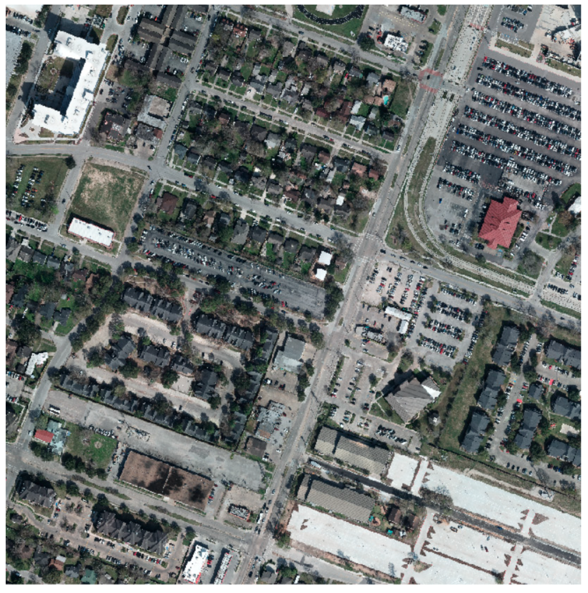
2.1. Multispectral LiDAR Data Acquisition

The airborne three-wavelength LiDAR, Optech Titan, provides multispectral information and has been successfully used in land classification and change detection, forestry biochemical parameters, bathymetry, and historical monument measurements. Titan is a single sensor with three active lasers of 532 nm (green), 1064 nm (NIR) and 1550 nm (MIR). Each beam is sampled at 300 kHz. However, it is to be noted that the Titan is not strictly a multispectral LiDAR, as the laser beams of its three channels are dispersed rather than being a single laser beam. Its specific parameters are shown in Table 1.
The study area is located on the University of Houston campus and its surrounding areas in the USA. The Optech Titan MW (14SEN/CON340) LiDAR sensor was used to acquire data during a flight mission on 16 February 2017. The flight plan parameters for Optech Titan are flying height: 500 m AGL, swath width: 445 m, overlap: 50%, and line spacing: 225 m. The equipment parameters are PRF: 175 kHz per channel (525 kHz total), scan frequency: 25 Hz, scan angle: ±26°, ±2° cut-off at processing. The acquired data are presented in LASer file format (LAS). The study area was rasterized from the Titan data, and the airborne image of the study area is shown in Figure 1.
The study area has an area size of 520 m × 520 m and has 4,436,481 point clouds, which are a subset of the acquired LiDAR dataset. The main land-use features in the study area are buildings, roads, paved parking lots, unpaved parking lots, shrubs, grass, vehicle, power lines, and impermeable surface. In this study, we focus on classifying roads, grass, buildings, trees, cars, and power lines from a complex urban environment. The number of multispectral point clouds corresponding to these features is shown in Table 2.

2.2. Multispectral LiDAR Data Processing
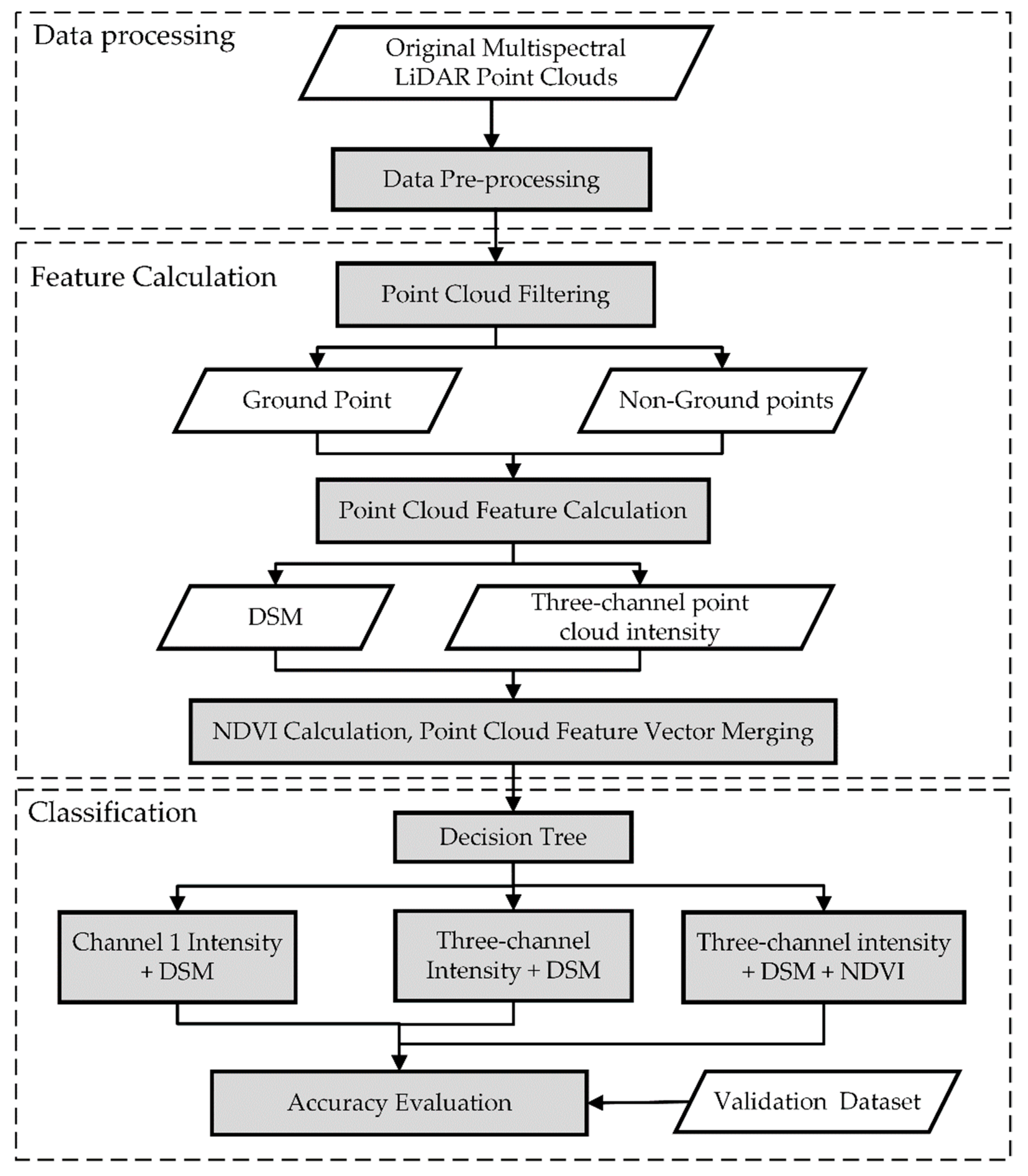
As the laser beams of channels C1 and C3 were tilted +3.5 and +7 degrees towards the nadir during the Titan data acquisition [37], not every point cloud in the Titan dataset has three channels of intensity data. In order to ensure the accuracy of the point cloud data, missing values without intensity information in the point cloud were removed. The point cloud intensity information from three separate channels is merged into one point cloud. Wichmann et al. [37] proposed a method for geometrically merging each point using its nearest neighbor intensity values in the channel point cloud, searching for the maximum distance between that point and the neighboring points and processing the data according to a distance threshold. This method allows three channels of intensity data for each point cloud in the processed point cloud. However, it may result in incorrect matches between points.
Another data-processing method is to, firstly, retain all point clouds from the three channels, and then to allocate the intensity information from the other channels to a single wavelength point cloud based on the hypothesis that there is a correlation between the spectral intensities of neighboring points [38]. For the point cloud data in one channel, five-point clouds in another channel are searched in a nearest-neighbor search, and then the spectral information of the point cloud in that channel is allocated using an inverse distance-weighted interpolation method. Finally, multispectral point cloud data with three-channel values would be obtained. Similarly, the method described above was refined in this study due to the different number of point clouds for the three channels of Titan data in the study area. Using the point cloud of channel 1 as a reference, the five-point clouds of the two nearest neighboring channels of each point cloud were searched to remove neighboring points at a distance greater than 1 m. The inverse distance-weighted interpolation method was then used to assign the point cloud of channel 1 based on the spectral intensity of the point clouds of channels 2 and 3 and to remove point clouds with no adjacent points within 1 m. This results in data containing three-channel values per point cloud and ensures the invariant number of point clouds in channel 1 before and after data processing. The processed reference multispectral data is shown in Figure 2.

3. Methods

The flow chart of classification is shown in Figure 3. The experiment classified the land cover of the study area into six classes: roads, grass, buildings, trees, cars, and power lines. A 3D point cloud-based feature method is used for the classification. The method involves filtering the point cloud after data pre-processing to split the point cloud in the study area into the ground and non-ground points. The land-use classes for the ground points include roads (impervious surfaces, such as car parks and concrete, are also classified as roads) and grass, while the land-use classes for the non-ground points contain buildings, trees (plants, such as shrubs, are classified as trees), cars, and power lines. Feature vectors, such as DSM and NDVI values for the study area, are obtained from the point clouds’ elevation information and intensity information. These feature vectors are classified using a decision tree supervised classification method. Three types of classification strategies are discussed in this study: Channel 1 of the multispectral LiDAR Titan is used to simulate single-band LiDAR data; Titan 3-channel data with DSM data from the study area; and Titan 3-channel data with DSM and NDVI data from the study area. Three different types of data are used to illustrate the potential of multispectral LiDAR for classification in complex urban areas. Finally, the classification results are evaluated based on the validation set. A confusion matrix is taken to measure the accuracy of the classification, and the overall accuracy and Kappa coefficient [39] are used to evaluate the accuracy of the classification. The detailed methodology is described in the following section.

3.1. Point Cloud Filtering

Point cloud filtering aims to divide the data into ground and non-ground points. There are several point cloud filtering algorithms, including slope-based methods [40], mathematical morphological filtering-based methods [41], and progressive encrypted triangular network TIN-based methods [42]. However, most of these algorithms are complex in parameter settings, and also too redundant for the flatter urban study area. In this experiment, the complex urban point cloud is divided into ground and non-ground points using a cloth simulation filter (CSF) algorithm [43] based on the cloth simulation of physical processes. While most traditional filtering algorithms take into account differences in slope or elevation changes to distinguish between ground and non-ground points, the ‘cloth’ filtering algorithm takes a relatively innovative approach to filtering by first flipping the point cloud and then assuming that a piece of cloth falls from above by gravity; the final cloth that falls is representative of the current digital surface model.

3.2. Produce DSM

DSM is a ground elevation model that demonstrates buildings, bridges, and trees on the land surface. DSM generation for our study area is interpolated using the inverse distance-weighting algorithm and the natural neighborhood algorithm. The inverse distance-weighting algorithm is used for the image element assignment method. This method is centered on the point to be interpolated for point cloud data. Discrete points are selected in appropriate local areas, and the elevation of the point p to be interpolated is settled using a weighted average [44]. The distance factor assigns weights to the discrete observations adjacent to the interpolated points according to their distance and the direction in the case of anisotropy. This is advantageous for generating DSMs by interpolating elevations from point clouds over large areas in complex urban areas [45].
Natural neighbor interpolation [46] is used to fill in the no data values for vacant values on the interpolated surface. This method interpolates by finding the nearest incoming sample set of the points interpolated and applying weights to these samples in proportion to the region’s size. Natural neighborhood interpolation is an interpolation method that limits the calculation of weights to the nearest range. The fundamental property of this interpolation algorithm is that it is local using only a subset of samples around the query point and ensuring that the interpolation height does not exceed the maximum height within the sample subset, providing good inheritance performance for local data characteristics, but making it difficult to take into account global data. Therefore, the method is used in experiments to perform interpolation operations on local vacancy values.

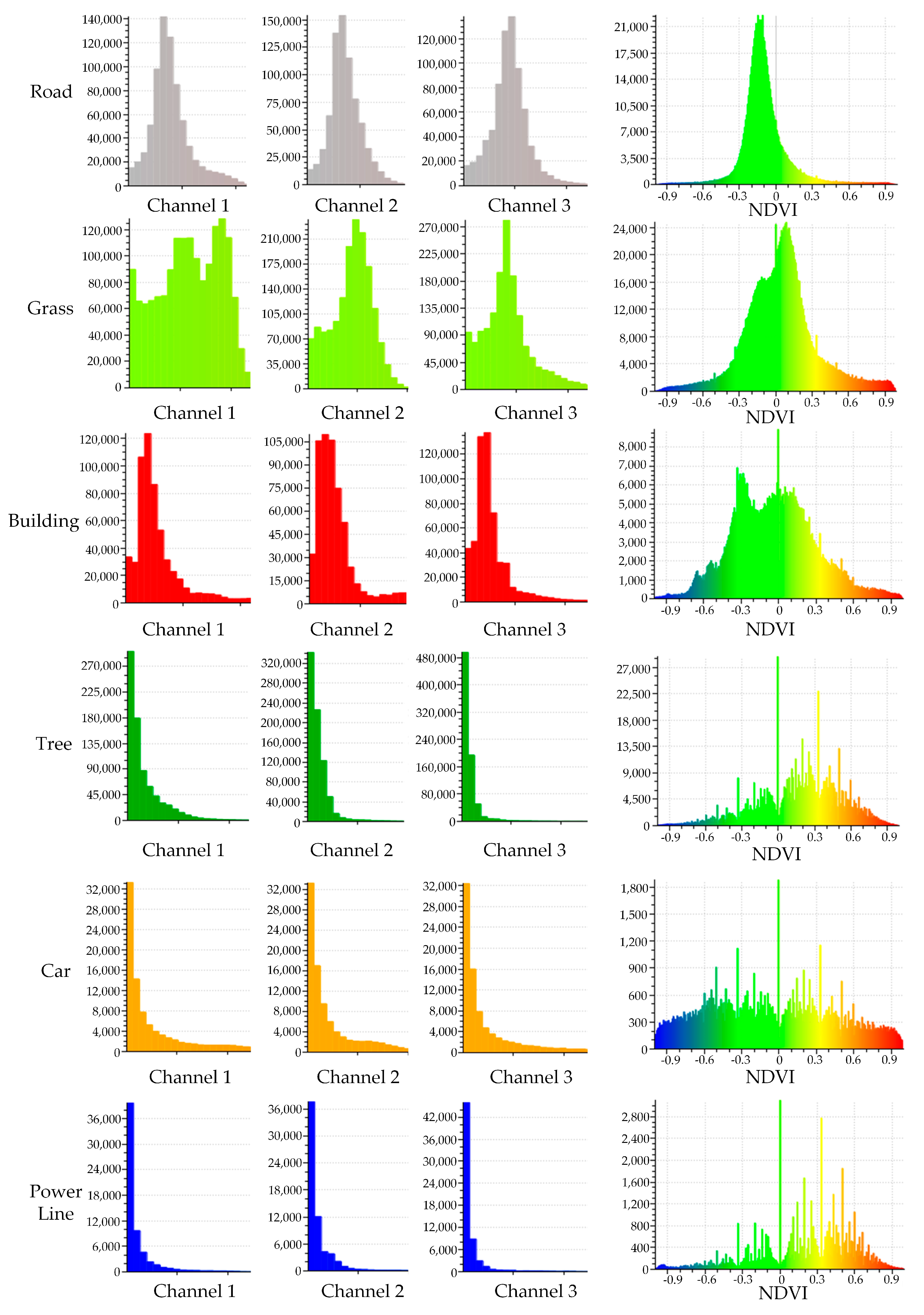
3.3. NDVI Calculation

The two feature classes, vegetation and buildings, differ in NIR and green; other differences in reflected energy in the NIR and green bands are distinguishable. Therefore, it is possible to distinguish between the different features based on the spectral characteristics of the Titan multispectral LiDAR data. The features can be classified according to their spectral characteristics in the Titan multispectral LiDAR data. Then, NDVI quantifies vegetation by measuring the difference between near-infrared (strong vegetation reflection) and red light (vegetation absorption). As Titan data are available in 1550 nm, 1064 nm, and 532 nm, NDVI values based on these three bands were calculated for classification [21,47].
NDVI NIR - MIR   = NIR MIR NIR + MIR
NDVI NIR - G = NIR G NIR + G
NDVI MIR - G = MIR G MIR + G
where MIR, NIR, and G represent the intensity values for Titan data channel 1, channel 2, and channel 3, respectively. The point cloud data is pre-processed so that each point cloud has a corresponding three NDVI values.

3.4. Feature Combination

After pre-processing the generated point cloud data, generating DSM, and calculating NDVI, the processing flow turns into merging point cloud feature vectors. The 1550 nm, 1064 nm, and 532 nm bands are acquired by Titan data. The reflectance of vegetation is stronger in the 1064 nm NIR band and lower in the green band at 532 nm, 1550 nm, and 1064 nm bands can be easily distinguished from the road to vegetation. The three-channel values of the Titan data are therefore used as intensity information—the generated DSM as the elevation information and the three calculated NDVIs as the spectral information are combined into a feature vector for classification. The combined eigenvectors for the three methods are shown below:
[ Channel   1 DSM ] [ Channel   1 Channel   2 Channel   3   DSM ] [ Channel   1 Channel   2 Channel   3 DSM NDVI MIR - G NDVI NIR - G NDVI NIR - MIR ]

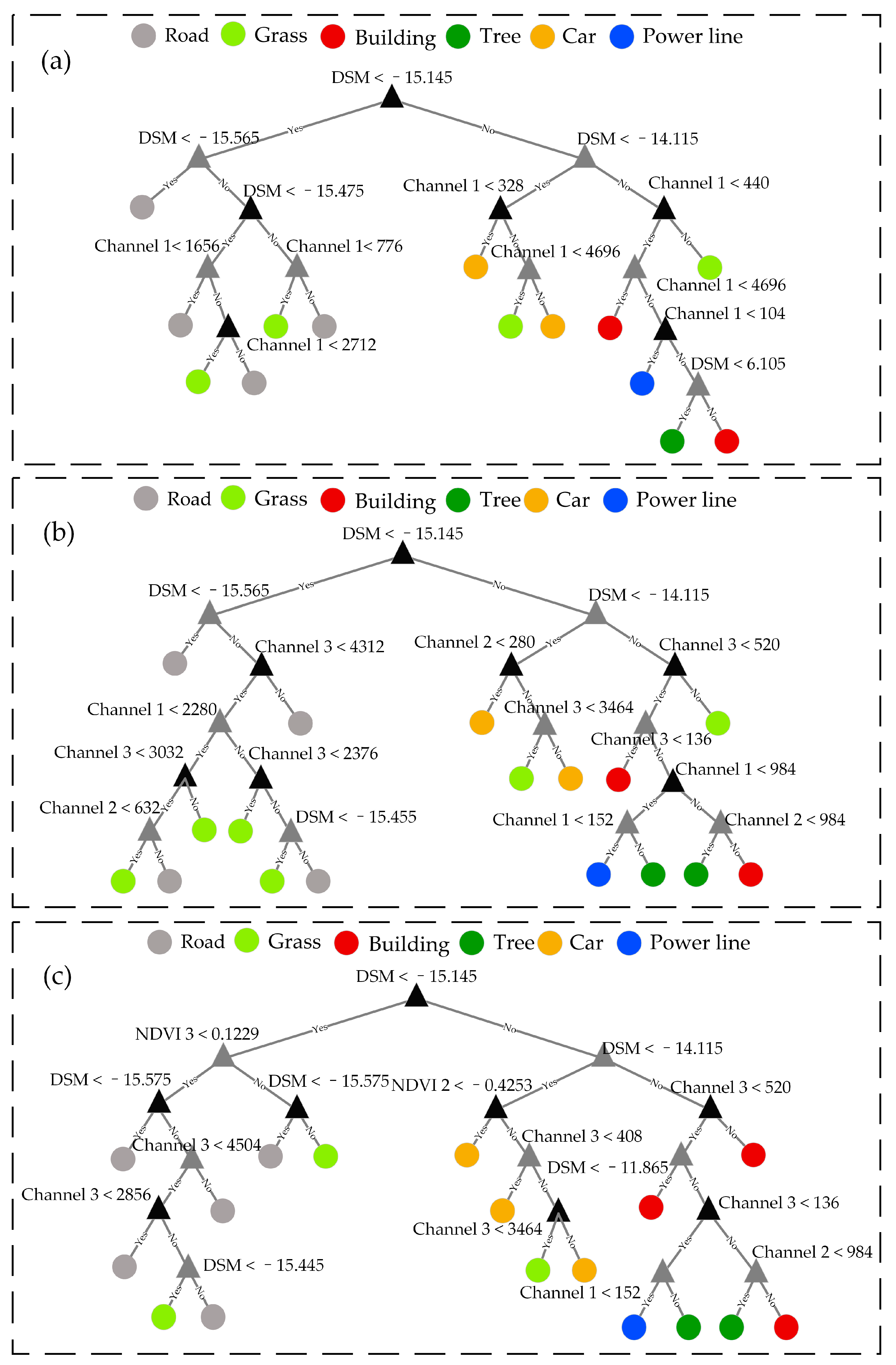
3.5. Decision Tree Construction

Decision tree [48] is a classic and widely used classifier. When a decision tree is constructed from training data, it can be used to efficiently classify untrained data. It has two main advantages: (1) it is readable and descriptive, which facilitates manual analysis; (2) it is efficient, as they only need to be constructed once and repeatedly used, with the maximum number of calculations per prediction not exceeding the depth of the decision tree.
The construction of the decision tree is a recursive process. Therefore, it is necessary to define conditions for recursion termination. Otherwise, the process will not be completed. A more intuitive approach is to stop when there is only one data type in each child node, but this usually makes the tree too large and leads to too many matching problems. Another possible approach is to make the number of records in the current node fall below a minimum threshold, in which case the construction of the decision tree stops and the corresponding classification is used as the classification of the current leaf node [49]. The decision trees generated by the above algorithm often lead to overfitting problems. In other words, the decision trees produce a low error rate for training data, but a high error rate when applied to test data. Therefore, several metrics were used in the experiments to evaluate the generated decision trees for the overfitting phenomena.
The Gini [50] measures whether a node is overfitted or not, which is different from the Gini coefficient in logistic regression. The smaller the Gini is, the better the decision tree will be when the nodes have more samples. The formula for its calculation is as follows:
Gini ( A j ) = 1   -   i = 1 n p ( i ) 2 ( j = 1 , 2 )
where p(i) is the proportion of each category = number of category i/total number. n is the category into which it is divided.
In information theory in probability statistics, entropy [51] is a measure that represents the uncertainty of a random variable, which is one of the criteria that reflect whether a decision tree is overfitted. When the entropy is higher, it means that the uncertainty of the random variable is more immense. The formula for its calculation is as follows:
Entropy = - i = 1 n P ( i )   ×   log 2 P ( i )
Similarly, P(i) represents the ratio of each category to the total, and n represents the category into which it is divided.
A fine decision tree is used to classify land use in the study area. A total of 100,000 × 6 data for the six categories in the study area were used to train the decision tree. The node thresholds of the decision tree are adjusted by means of expert experience and manual intervention to obtain the optimal decision tree.

4. Results

In order to confirm the potential of multispectral LiDAR for the classification of complex urban areas, three comparable methods are set up. Method (a) represents a classification using the Channel 1 band of Titan data plus DSM data to simulate the situation of the single-band LiDAR in classification. Method (b) represents a classification using Titan three-channel intensity data plus DSM data from the study area to illustrate the role of intensity information and elevation information in this landscape. Method (c) represents a classification using Titan three-channel data plus DSM data from the study area and calculated three NDVI data. A focused analysis of this method was carried out to show the advantages and potential of multispectral LiDAR in the classification of complex cities. The specific classification strategies are shown in Table 3.

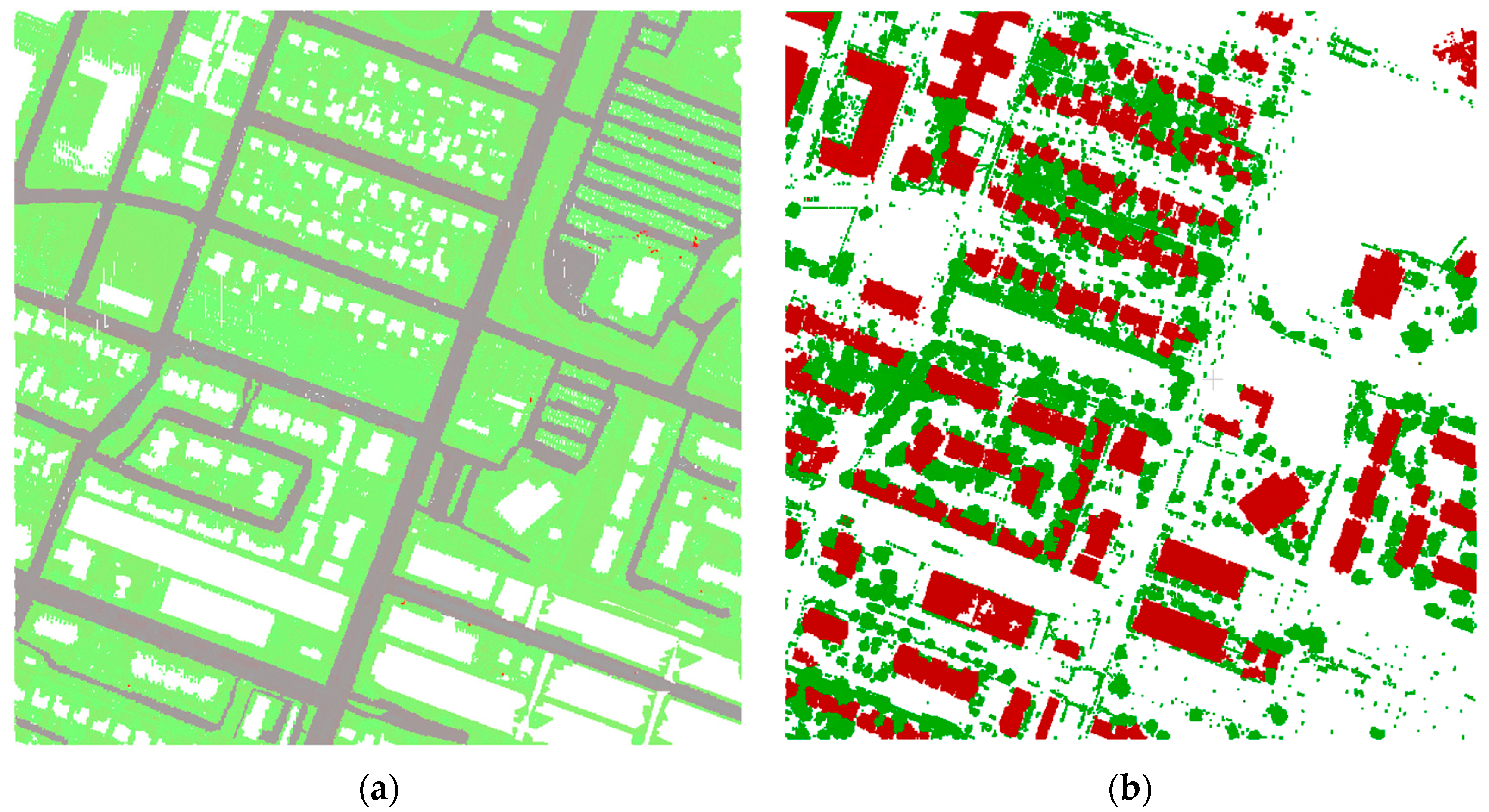
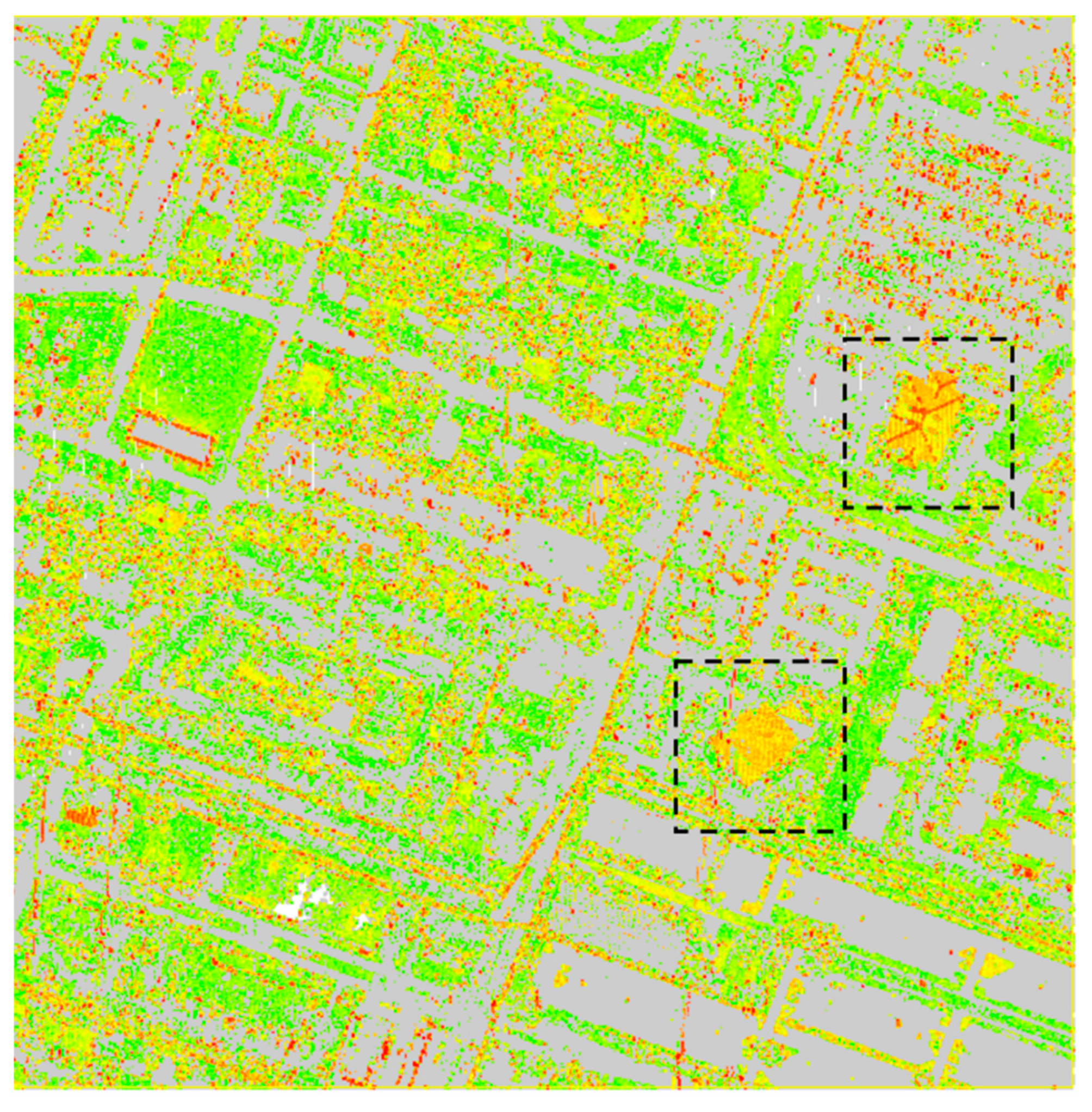
4.1. Point Cloud Filtering Influence on Classification

In order to reduce the influence of complex urban areas on the classification results, the area’s point cloud is first classified into ground and non-ground points. The main parameters of CSF filtering based on cloth simulation are the cloth resolution, the maximum number of iterations, and the classification threshold. The higher the fabric resolution, the more noise points are separated from the point cloud. According to previous research, setting the classification threshold to 0.5 with 500 iterations provides optimal parameters for achievable results [52]. After pre-processing the training set sample selection, the ground and non-ground points have different land-use classes after point cloud filtering. This process dramatically reduces the workload when using the classifier later, and the higher accuracy of the point cloud filtering allows for more accurate classification. The number of point clouds has not changed after point cloud filtering and only contains two categories of ground points and non-ground points in Figure 4.
The filtering used in the experiments is based on the CSF filtering of the cloth simulation. As shown from Figure 4, the filtering can accurately delineate ground and non-ground boundaries. The study area is easy to identify due to the distribution pattern of roads and grass, while the spatial characteristics between buildings and trees are more complex and difficult to distinguish. The identification of non-ground points is the focus of point cloud classification. The filtered point clouds were also denoised when ticking the training set samples. This prevents the presence of class uncertainty in some small, sparse point clouds from affecting the classification results. In addition, the training set samples are chosen evenly for the classification of land use categories, with the same number of training sets for each type of sample. For example, the training set is uniformly selected and identical due to the significant differences in spectral information between houses with different colored roofs.

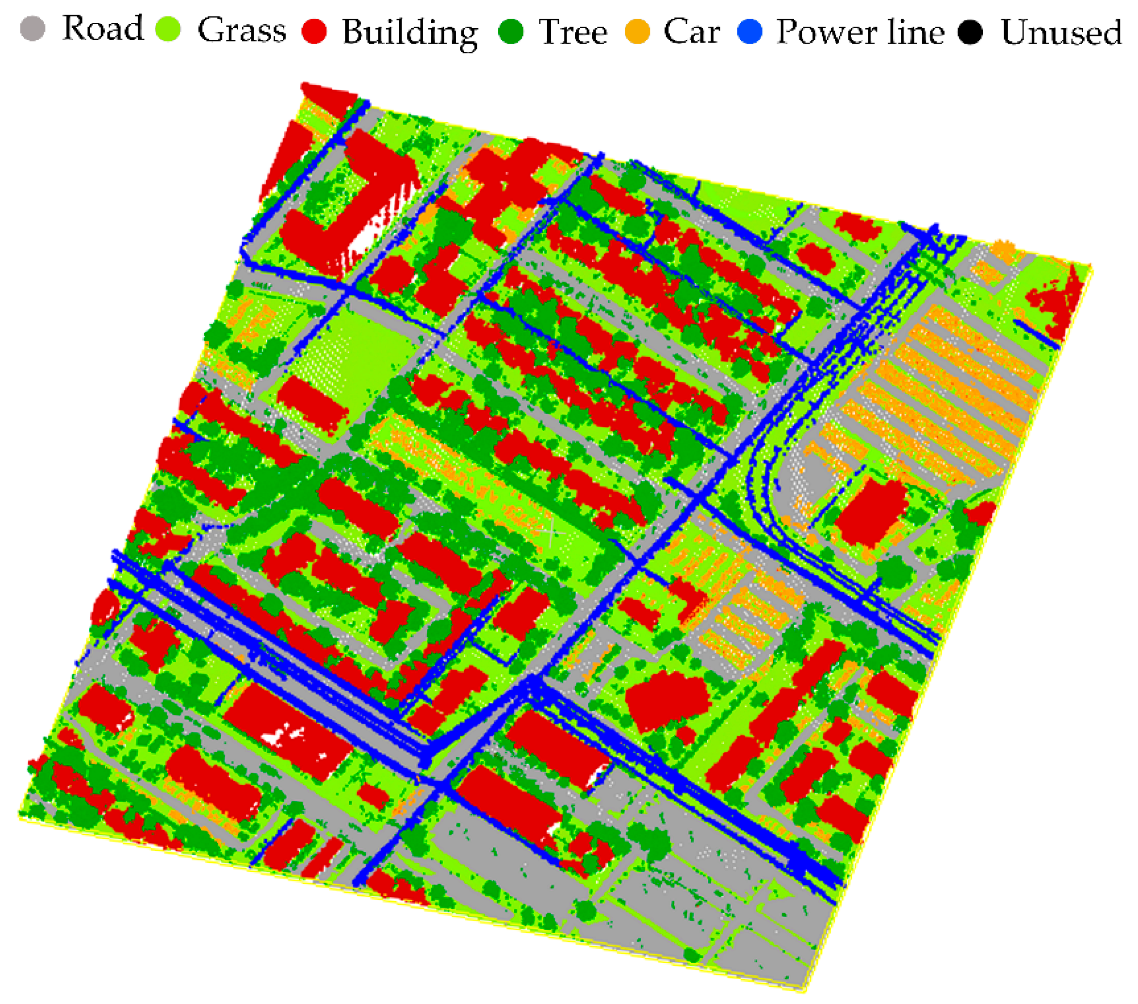
4.2. Decision Tree Classification

After selecting the training samples, the fine decision tree classifier constructed from the three methods inputs was divided in Figure 5. The training set was divided into five parts, four-fifths of which were used for training, while the rest were used as a test set to verify the accuracy of the classifier. Method (a) has a depth of 43 levels, and its self-validation accuracy is 72.1%; method (b) has a depth of 37 levels, and its self-validation accuracy is 80.6%; and method (c) has a depth of 41 levels, and its self-validation accuracy is 91.2%.
The Gini coefficients and entropy of the three constructed decision trees are shown in Table 4. The Gini coefficients and entropy to whether the decision tree generated by the algorithm is overfitted. Method (a) has the largest Gini coefficient and entropy, while method (c) has the smallest. The main reason here is that only a single band of data is used in method (a), and this training set achieves a certain level of accuracy through overfitting. Data overfitting occurs in method (a). In contrast, for project (c), the constructed decision tree’s Gini index and entropy values are lower. The results of using this classifier are better, indicating that a classifier-like decision tree is suitable for application in complex urban landscapes. The two main reasons for this are: (1) noisy data; there is noisy data in the training data, and some nodes of the decision tree have noisy data as segmentation criteria, resulting in the decision tree failing to represent the accurate data. (2) Lack of representative data: the training data does not contain all representative data, resulting in a certain class of data not being well-matched, which can be derived by observing the confusion matrix analysis. Similarly, this cause plays a decisive role in constructing the decision tree, reflected in method (a) and method (c).
Where method (c) constructs a decision tree with small Gini coefficients and entropy values within acceptable limits, because project (c) uses elevation information, intensity information, and spectral information from multispectral LiDAR point clouds, there are no lack of data or overfitting in the construction of these supervised classification classifiers. In contrast, single-band LiDAR in classifiers such as decision trees can cause the overfitting of the classifier due to the inclusion of elevation information and single-band intensity information, which demonstrates that multispectral LiDAR has a wealth of information that can be applied in land-cover classification.

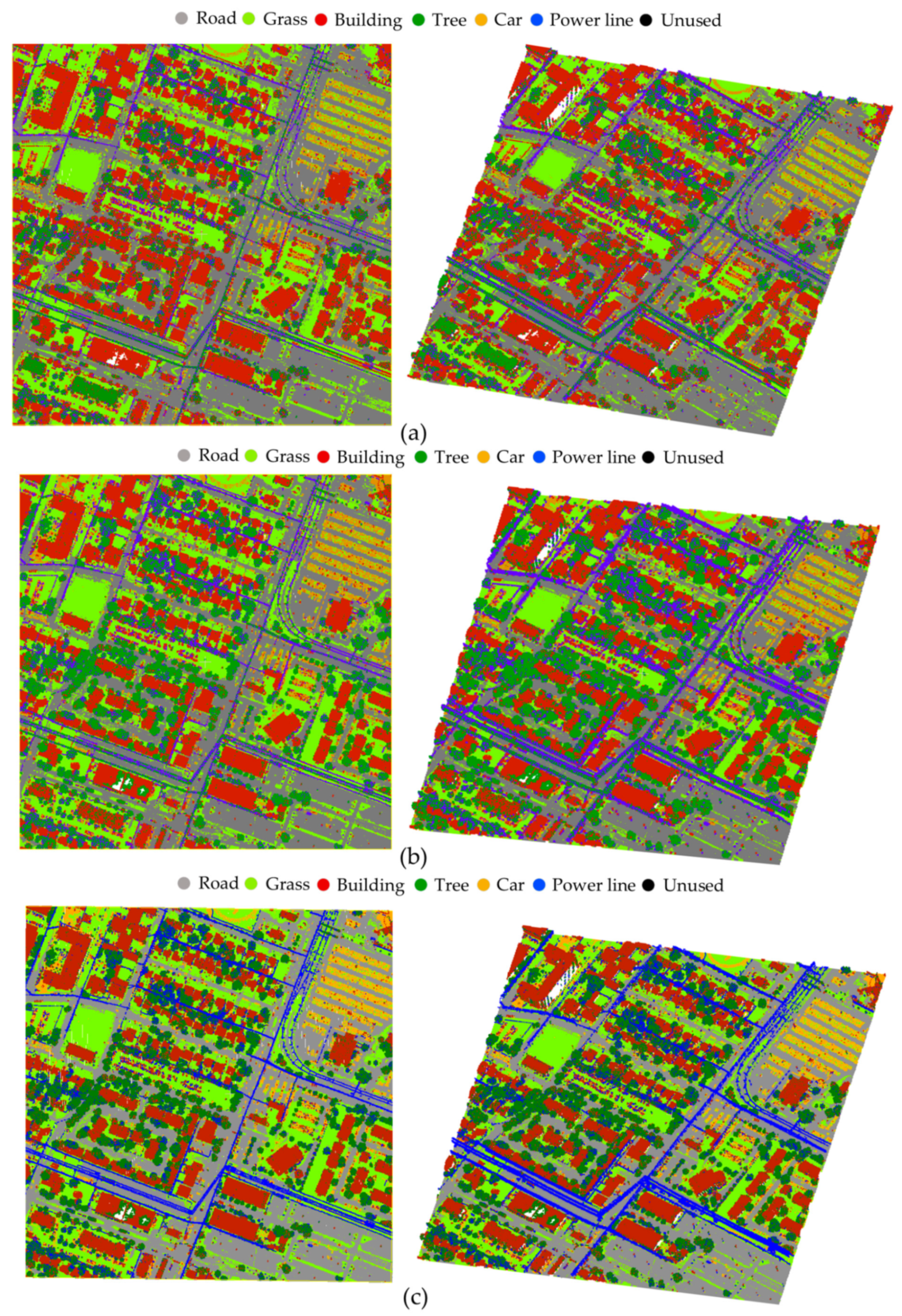
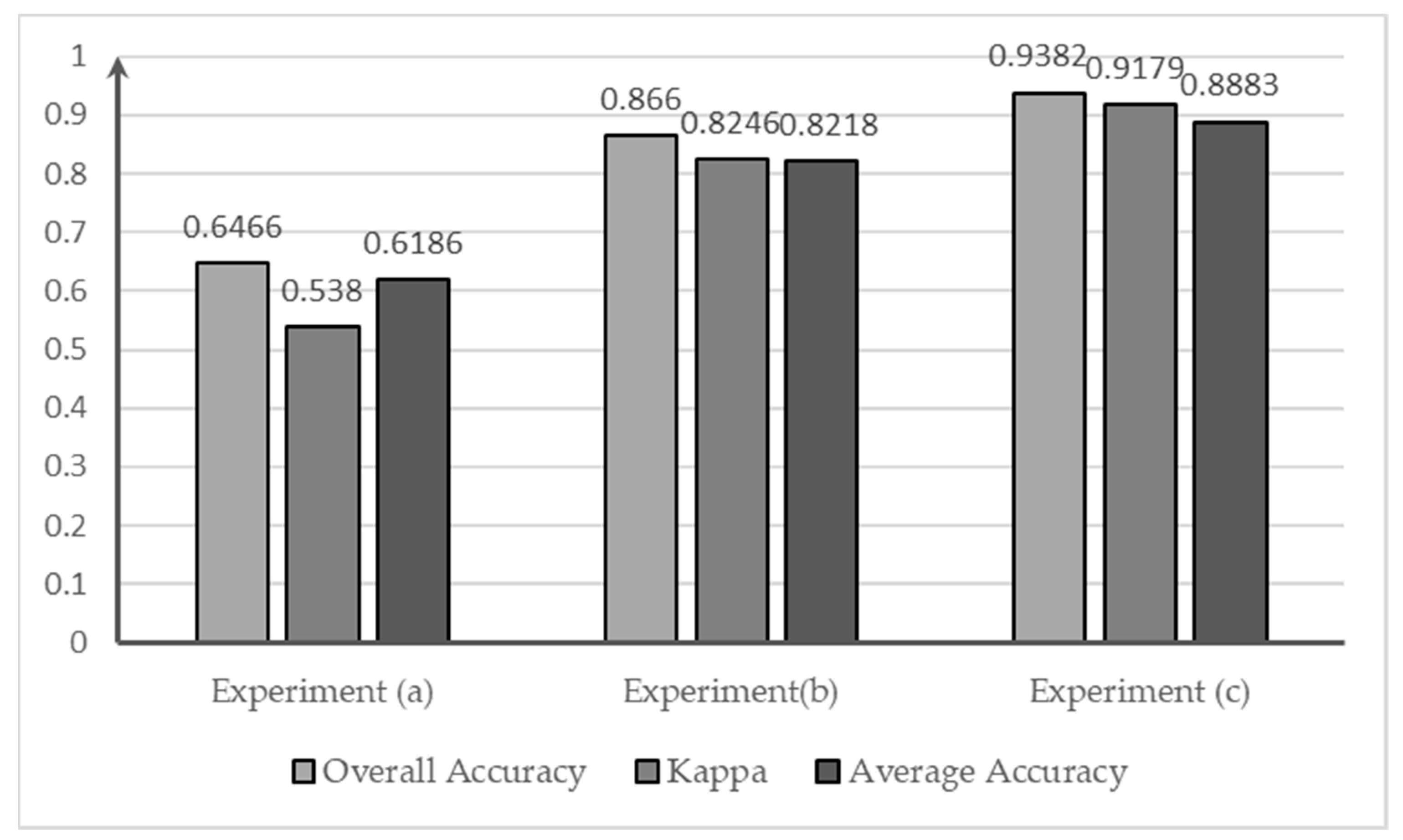
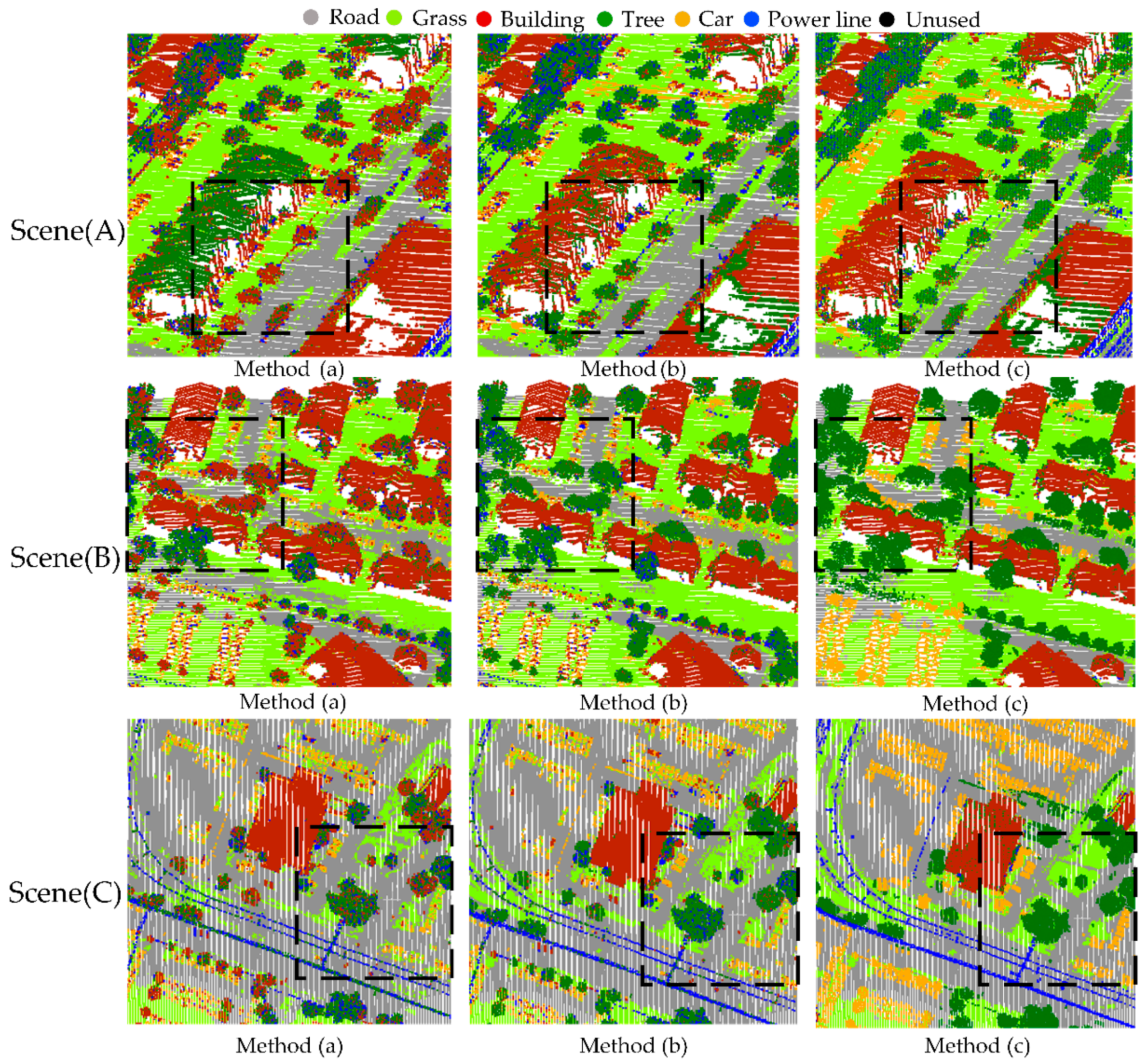
4.3. Comparison of Classification Results

The three controlled classifications include point cloud data pre-processing, DSM generation and NDVI calculation, applying the elevation information, intensity information, and spectral information of the multispectral point cloud data, respectively. The point clouds are first pre-processed, using a nearest-neighbor search method for data with missing intensity data. CSF filtering based on cloth simulation is then used for point cloud filtering. The point cloud filtering divides the data of the study area into ground and non-ground points. Next, the point cloud feature vectors are extracted, the elevation information of the point cloud is produced as DSM, and the three-channel intensity data of the Titan data are combined. Due to the high reflectance of vegetation in the NIR and green bands, the border between roads and grass (buildings and trees) was delineated by NDVI. Three NDVIs, according to the three channels of Titan data, are computed; these three data are fused into point cloud feature vectors. Three controlling methods, using fine decision trees in order to obtain different LiDAR classification results, were designed. In this way, the advantages and potential of multispectral LiDAR for complex urban land-use classification are shown. The classification results of the three methods are shown in Figure 6. The experimental results show that the multispectral LiDAR point cloud (method (c)) based on intensity, elevation, and spectral information is more advantageous than the other two classification data, especially for delineating the boundaries between roads and grassland. Among the three methods, it was found that the elevation and intensity information of the point clouds only played an auxiliary role in land-use classification. However, the intensity information of the multi-channel can be used to classify features with large differences in intensity between feature classes, such as buildings and trees as well as roads and grass. However, due to the ignoring of spectral information, the classification of features with large spectral differences between the same categories is not as effective as it could be. In contrast, the classification results in method (c) demonstrated that cars with large differences in colors have large variability in intensity information and a large difference in spatial distribution, which allows them to be classified as cars by using spectral information. Table 5, Table 6 and Table 7 provide confusion matrices, total overall accuracy, and Kappa coefficients based on the three method data.
Method (a), method (b) and method (c) correspond to an overall accuracy of 64.66%, 86.60%, and 93.82%, respectively. Their Kappa coefficients are 0.5380, 0.8246, and 0.9179, respectively. Compared with previous research [29,53] on 3D point cloud delineation, based on threshold segmentation and supervised classification, the accuracy of classification is improved, and the accuracy and completeness of feature boundary extractions in complex urban classification are ensured.

5. Discussion

In order to analyze the performance of multispectral LiDAR for land-use classification in complex urban landscapes, three methods are taken in this study to illustrate this against each other. There are two main sources of error in this experiment: the first is that point cloud filtering has an impact on the accuracy of the classification results. Although the aim of the experiments with point cloud filtering is to be the first to separate ground points from non-ground points, and despite the use of CSF filtering suitable for complex urban areas, there is no guarantee that the filtering accuracy is completely correct. After point cloud filtering, there is a phenomenon of misclassifying ground points as non-ground points and vice versa. This error is further exaggerated in the training set samples due to the sample selection method used for the study, making it not completely accurate. The second one is that the multispectral LiDAR data were collected in winter when the vegetation is not in as lush a state as during the summer growing season. This results in smaller NDVI values for some vegetation, which may be the same as the NDVI of some spectrally similar buildings. On the other hand, the majority of trees in the study area are evergreen vegetation, with less seasonal vegetation. NDVI can help to distinguish vegetation from non-vegetation to some extent in winter. There is no denying that spectral information, such as NDVI, plays an essential role in classification. The three NDVI values calculated in method (c) have some deviation, as shown in Figure 7, for NDVI NIR - G ; when extracting NDVI NIR - G values greater than 0, as its value gets larger, it should correspond to lush vegetation, and a building with a yellow roof. This indicates that the calculated NDVI may not be suitable for this study area, and a better multispectral LiDAR-based vegetation cover index should be proposed in future work to reflect its spectral characteristics.
Overall, the classification results from the three methods confirm the potential of multispectral LiDAR for land-use classification in complex urban landscapes. A comparison of the classification accuracy of the three methods is shown in Figure 8. The study area selected for the experiments covers a large area with complex land-use types, possessing various features and representative land-use categories. Using multispectral LiDAR to classify the area’s land use into roads, grass, buildings, trees, cars, and power lines, the method achieved an overall classification accuracy of 93.82%. The method, which uses only the Titan Channel 1 single-band LiDAR and DSM classification in method (a), often fails to yield accurate land-use classification results due to the data limitations of the single-band LiDAR, which can only rely on single-band intensity information or radar echo information for classification. In the case of the classification for six types of features, spectral information is missing. It is difficult to distinguish among the six categories. In particular, for the two feature categories of power lines and trees with similar values in the Channel 1 band at two points, the user accuracy is only 16.24% and 54.61%. In method (b), although the intensity data of the three channels and elevation information such as DSM were used, the classification accuracy was still plain, especially for the cars and power lines feature categories, where the user accuracy is only 68.59% and 29.77%. The importance of adding elevation information, the difference in elevation between the road and building as well as the grass and tree categories can be used to clearly delineate their categories. However, there are still some misclassifications between buildings and roads, grass, and trees. The main reason might be that the elevation of the study area shows an increasing tendency from the southeast to the northwest, which would influence the lower buildings and shrubs to be misclassified. Their elevation information is similar; it is still difficult to distinguish them by intensity information alone, and the spectral information needs to be added to delineate the boundaries between the low buildings and shrubs. The elevation information, intensity information and spectral information of the point clouds were used in method (c). The consideration of the NDVI index made it possible to classify between cars and buildings, as well as trees and power lines, which are classes with similar intensity information. In Figure 6, the classification using multispectral LiDAR shows that the boundaries between the classes are more distinct than in the other two methods and that the continuity of the classified features is improved. For the classification of trees, method (c) shows fewer noise points of other classes, especially in the complex area where buildings and trees overlap. In addition, the classification of power lines showed continuous lines without noise from surrounding trees and buildings.
In particular, the results of the comparative methods demonstrate the efficiency of LIDAR intensity, height, and spectral information in urban land-use classification. After using DSM with multi-channel intensity information for classification, the overall accuracy was improved by more than 20%. Then, after adding spectral information for classification in method (c), the overall accuracy was improved by less than 10%, but the accuracy used for some classes was significantly increased. One of the most significant increases was for power lines, where the user accuracy increased by almost 50%. In addition, the classification of vehicles was also made better. As mentioned earlier, point cloud filtering and the calculation of NDVI are two sources of classification error. Approximately 15% of the power line point clouds were incorrectly classified as buildings and trees. This resulted in a user accuracy of only 74.89% in method (c). Similarly, about 14.1% of the vehicle point clouds were misclassified, mainly as roads and trees.
Furthermore, in order to illustrate the potential and advantages of spectral information in land-use classification, histograms of the six feature classes of the Titan three-channel information (1550 nm, 1064 nm, and 532 nm) and NDVI are shown in Figure 9. The peaks of each feature type in the study area can be observed. The rationale for the classification is actually to find heterogeneity between these feature classes on a particular feature. Most of the features in the study area show a single peak distribution, which makes it difficult for the classifier to classify features based solely on the intensity information of the three channels. For some feature classes with similar intensity information across the three channels, such as roads and grasslands, the distribution is similar between Channel 2 and Channel 3, which leads to misclassification. The elevation distribution in the study area demonstrates a southeast to northwest increase, which may also make it difficult to separate land-use categories if elevation information is added. For example, buildings at lower elevations and roads at higher elevations have similar intensity information. At this point, because their elevation information is so similar, errors in classification are created. When adding the spectral information, the values of NDVI were calculated using the intensity information from the three channels; it can be observed in Figure 9 that the six features are dramatically different in terms of NDVI and are able to classify artificial features and vegetation. Therefore, in our experiments to illustrate the advantages of multispectral LiDAR in land use, we took three NDVIs based on the three-channel intensity information to differentiate the features. We found that NDVI NIR - G can effectively classify roads and grass, and NDVI NIR - MIR can classify buildings and trees. These NDVIs play a significant role in classifying and illustrating the multispectral LIDAR advantages in this complex urban land-use classification.
In detail, the differences among the three methods in the specific details of the classification are shown in Figure 10. The differences evident in the classification results have been selected to demonstrate the potential of multispectral LiDAR in the classification of complex cities. For scene (a), this area is the primary road in the city, and the buildings and trees are on both sides. Method (a) and method (b) use only intensity and elevation information; the lack of spectral information made it hard to distinguish between the roofs of buildings and trees, and most of the buildings and trees are incorrectly classified with each other. There also existed cases of cars being misclassified as buildings. In contrast, the land-use types can be better separated in method (c), and the extracted land classes are almost free from other classes of noise points, maintaining an excellent contour and continuity. In scene (b), similar to scene (a), the lack of spectral data for classification can cause errors between building and tree categories. The usefulness of the spectral information is highlighted even more in scene (c). The spectral information mainly affects the separation between vegetation and buildings. The addition of spectral information in method (c) makes the classification of cars relatively easy. Its effectiveness is also shown by the ability to accurately classify the boundaries of trails in grass. Due to the insufficient point cloud density of LiDAR in complex urban features and the fact that classification can only rely on intensity information and elevation information, this can lead to difficulties in differentiating between feature categories with large spectral differences, resulting in a significant increase in classification errors. Overall, the three methods taken in this thesis effectively illustrate the advantages and potential development possibilities of multispectral LiDAR for the classification of complex urban land use. Multispectral LiDAR allows for more accurate classification due to its multi-channel spectral characteristics.

6. Conclusions

This research confirmed and discussed the potential of multispectral LiDAR for the classification of complex urban areas. The intensity values of the three channels of Optech Titan data were first assigned to a point cloud using a nearest-neighbor search method. After point cloud pre-processing, ground filtering was applied to the point cloud in the study area using CSF filtering based on cloth simulation to obtain ground points and non-ground points. Training samples of roads and grass were selected from the ground points, and training samples of buildings, trees, cars, and power lines were selected from the non-ground points. A DSM of the study area using inverse distance-weighting algorithms was generated. Then, three NDVIs were calculated for point cloud classifications based on three bands of Titan data. The elevation, intensity, and spectral information of the multispectral LiDAR point clouds were combined into three-point cloud feature vectors for target classification. The first types of data are Channel 1 of the Titan data, simulating a single-band LiDAR used for point cloud classification of the study area; the second types of data are the point cloud of the three channels of the Titan data plus the generated DSM; the third types of data are the three channels of the Titan data plus the DSM and the three NDVIs. The classifier chosen for the experiment was a decision tree classification for the multispectral LiDAR composition. The decision tree classifier trained on the data had no overfitting phenomenon. The overall accuracy of the final classification is 64.66%, 86.60%, and 93.82% for the three data types, respectively. Comparing the classification results of the three data highlights that elevation information, such as DSM, plays a role in the point cloud classification, while the importance of NDVI, calculated by the multispectral LIDAR, is excellent in complex landscapes.
Multispectral LiDAR is currently being upgraded to Hyperspectral LiDAR. This 3D point cloud, containing a large amount of spectral information, can be effectively utilized to classify complex urban areas, with further potential that is yet to be uncovered in remote-sensing monitoring.

Author Contributions

Conceptualization, B.L., W.G. and J.Y.; methodology, B.L. and J.Y.; software, B.L. and J.Y.; validation, B.L., J.Y. and S.S. (Shuo Shi); formal analysis, B.L., J.Y., S.S. (Shuo Shi), S.S. (Shalei Song), A.W. and L.D.; investigation, B.L. and J.Y.; resources, B.L., J.Y., S.S. (Shuo Shi) and W.G.; data curation, B.L. and J.Y.; writing—original draft preparation, B.L. and J.Y.; writing—review and editing, B.L., J.Y., S.S. (Shuo Shi), S.S. (Shalei Song), A.W. and L.D.; visualization, B.L. and J.Y.; supervision, J.Y.; project administration, J.Y.; funding acquisition, J.Y., S.S. (Shuo Shi) and S.S. (Shalei Song); All authors have read and agreed to the published version of the manuscript.

Funding

This research was funded by the National Key R&D Program of China (2018YFB0504500), the National Natural Science Foundation of China (41801268, 41971307, 42171347).

Data Availability Statement

No new data were created or analyzed in this study. Data sharing is not applicable to this article.

Acknowledgments

The authors thank the Hyperspectral Image Analysis Lab at the University of Houston for providing the original Optech Titan data.

Conflicts of Interest

The authors declare no conflict of interest.

References

  1. Petropoulos, G.P.; Arvanitis, K.; Sigrimis, N. Hyperion hyperspectral imagery analysis combined with machine learning classifiers for land use/cover mapping. Exp. Syst. Appl. 2012, 39, 3800–3809. [Google Scholar] [CrossRef]
  2. Pal, M. Support vector machine-based feature selection for land cover classification: A case study with DAIS hyperspectral data. Int. J. Remote Sens. 2006, 27, 2877–2894. [Google Scholar] [CrossRef]
  3. Wei, G.; Shuo, S.; Biwu, C.; Lei, S.S.; Zheng, N.; Cheng, W.; Haiyan, G.; Wei, L.; Shuai, G.; Yi, L.; et al. Development of Hyperspectral Lidar for Earth Observation and Prospects. J. Remote Sens. 2021, 25, 501–513. [Google Scholar]
  4. Zou, X.; Zhao, G.; Li, J.; Yang, Y.; Fang, Y. 3D land cover classification based on multispectral lidar point clouds. Int. Arch. Photogramm. Remote Sens. Spat. Inf. Sci. 2016, 41, 741–747. [Google Scholar] [CrossRef] [Green Version]
  5. Yan, W.Y.; Shaker, A.; El-Ashmawy, N. Urban land cover classification using airborne LiDAR data: A review. Remote Sens. Environ. 2015, 158, 295–310. [Google Scholar] [CrossRef]
  6. Axelsson, A.; Lindberg, E.; Olsson, H. Exploring multispectral ALS data for tree species classification. Remote Sens. 2018, 10, 183. [Google Scholar] [CrossRef] [Green Version]
  7. Grebby, S.; Cunningham, D.; Naden, J.; Tansey, K. Application of airborne LiDAR data and airborne multispectral imagery to structural mapping of the upper section of the Troodos ophiolite, Cyprus. Int. J. Earth Sci. 2012, 101, 1645–1660. [Google Scholar] [CrossRef] [Green Version]
  8. Yang, J.; Yang, S.; Zhang, Y.; Shi, S.; Du, L. Improving characteristic band selection in leaf biochemical property estimation considering correlations among biochemical parameters based on the PROPSECT-D model. Opt. Express 2021, 29, 400–414. [Google Scholar] [CrossRef] [PubMed]
  9. Priestnall, G.; Jaafar, J.; Duncan, A. Extracting urban features from LiDAR digital surface models. Comput. Environ. Urban Syst. 2000, 24, 65–78. [Google Scholar] [CrossRef]
  10. Rubinowicz, P.; Czynska, K. Study of city landscape heritage using LiDAR data and 3D-city models. Int. Arch. Photogramm. Remote Sens. Spat. Inf. Sci. 2015, 40, 1395. [Google Scholar] [CrossRef] [Green Version]
  11. Ladefoged, T.N.; McCoy, M.D.; Asner, G.P.; Kirch, P.V.; Puleston, C.O.; Chadwick, O.A.; Vitousek, P.M. Agricultural potential and actualized development in Hawai’i: An airborne LiDAR survey of the leeward Kohala field system (Hawai’i Island). J. Archaeol. Sci. 2011, 38, 3605–3619. [Google Scholar] [CrossRef]
  12. Chase, A.S.; Weishampel, J. Using LiDAR and GIS to investigate water and soil management in the agricultural terracing at Caracol, Belize. Adv. Archaeol. Pract. 2016, 4, 357–370. [Google Scholar] [CrossRef]
  13. Buján, S.; González-Ferreiro, E.; Reyes-Bueno, F.; Barreiro-Fernández, L.; Crecente, R.; Miranda, D. Land Use Classification from Lidar Data and Ortho-Images in a Rural Area. Photogramm. Rec. 2012, 27, 401–422. [Google Scholar] [CrossRef]
  14. Man, Q.; Dong, P.; Guo, H. Pixel-and feature-level fusion of hyperspectral and lidar data for urban land-use classification. Int. J. Remote Sens. 2015, 36, 1618–1644. [Google Scholar] [CrossRef]
  15. Uthe, E.E. Application of surface based and airborne lidar systems for environmental monitoring. J. Air Pollut. Control Assoc. 1983, 33, 1149–1155. [Google Scholar] [CrossRef]
  16. Guo, J.; Liu, B.; Gong, W.; Shi, L.; Zhang, Y.; Ma, Y.; Zhang, J.; Chen, T.; Bai, K.; Stoffelen, A.; et al. Technical note: First comparison of wind observations from ESA’s satellite mission Aeolus and ground-based radar wind profiler network of China. Atmos. Chem. Phys. 2021, 21, 2945–2958. [Google Scholar] [CrossRef]
  17. Shi, T.; Han, G.; Ma, X.; Gong, W.; Chen, W.; Liu, J.; Zhang, X.; Pei, Z.; Gou, H.; Bu, L. Quantifying CO2 Uptakes Over Oceans Using LIDAR: A Tentative Experiment in Bohai Bay. Geophys. Res. Lett. 2021, 48, e2020GL091160. [Google Scholar] [CrossRef]
  18. Wang, W.; He, J.; Miao, Z.; Du, L. Space-Time Linear Mixed-Effects (STLME) model for mapping hourly fine particulate loadings in the Beijing-Tianjin-Hebei region, China. J. Clean. Prod. 2021, 292, 125993. [Google Scholar] [CrossRef]
  19. Li, H.; Gu, H.; Han, Y.; Yang, J. Fusion of high-resolution aerial imagery and lidar data for object-oriented urban land-cover classification based on svm. In Proceedings of the ISPRS Workshop on Updating Geo-Spatial Databases with Imagery & the 5th ISPRS Workshop on DMGISs, Urumqi, China, 28–29 August 2007. [Google Scholar]
  20. Zhou, W. An object-based approach for urban land cover classification: Integrating LiDAR height and intensity data. IEEE Geosci. Remote Sens. Lett. 2013, 10, 928–931. [Google Scholar] [CrossRef]
  21. Morsy, S.; Shaker, A.; El-Rabbany, A. Multispectral LiDAR data for land cover classification of urban areas. Sensors 2017, 17, 958. [Google Scholar] [CrossRef] [Green Version]
  22. Dai, W.; Yang, B.; Dong, Z.; Shaker, A. A new method for 3D individual tree extraction using multispectral airborne LiDAR point clouds. ISPRS J. Photogramm. Remote Sens. 2018, 144, 400–411. [Google Scholar] [CrossRef]
  23. Ekhtari, N.; Glennie, C.; Fernandez-Diaz, J.C. Classification of airborne multispectral lidar point clouds for land cover mapping. IEEE J. Sel. Top. Appl. Earth Obs. Remote Sens. 2018, 11, 2068–2078. [Google Scholar] [CrossRef]
  24. Brennan, R.; Webster, T. Object-oriented land cover classification of lidar-derived surfaces. Can. J. Remote Sens. 2006, 32, 162–172. [Google Scholar] [CrossRef]
  25. Song, J.-H.; Han, S.-H.; Yu, K.; Kim, Y.-I. Assessing the possibility of land-cover classification using lidar intensity data. Int. Arch. Photogramm. Remote Sens. Spat. Inf. Sci. 2002, 34, 259–262. [Google Scholar]
  26. Charaniya, A.P.; Manduchi, R.; Lodha, S.K. Supervised parametric classification of aerial lidar data. In Proceedings of the 2004 Conference on Computer Vision and Pattern Recognition Workshop, Washington, DC, USA, 27 June–2 July 2004; p. 30. [Google Scholar]
  27. Lodha, S.K.; Kreps, E.J.; Helmbold, D.P.; Fitzpatrick, D. Aerial LiDAR data classification using support vector machines (SVM). In Proceedings of the Third International Symposium on 3D Data Processing, Visualization, and Transmission (3DPVT’06), Chapel Hill, NC, USA, 14–16 June 2006; pp. 567–574. [Google Scholar]
  28. Antonarakis, A.; Richards, K.S.; Brasington, J. Object-based land cover classification using airborne LiDAR. Remote Sens. Environ. 2008, 112, 2988–2998. [Google Scholar] [CrossRef]
  29. Singh, K.K.; Vogler, J.B.; Shoemaker, D.A.; Meentemeyer, R.K. LiDAR-Landsat data fusion for large-area assessment of urban land cover: Balancing spatial resolution, data volume and mapping accuracy. ISPRS J. Photogramm. Remote Sens. 2012, 74, 110–121. [Google Scholar] [CrossRef]
  30. Onojeghuo, A.O.; Onojeghuo, A.R. Object-based habitat mapping using very high spatial resolution multispectral and hyperspectral imagery with LiDAR data. Int. J. Appl. Earth Obs. Geoinf. 2017, 59, 79–91. [Google Scholar] [CrossRef]
  31. Gong, W.; Song, S.; Zhu, B.; Shi, S.; Li, F.; Cheng, X. Multi-wavelength canopy LiDAR for remote sensing of vegetation: Design and system performance. ISPRS J. Photogramm. Remote Sens. 2012, 69, 1–9. [Google Scholar]
  32. Sun, J.; Shi, S.; Chen, B.; Du, L.; Yang, J.; Gong, W. Combined application of 3D spectral features from multispectral LiDAR for classification. In Proceedings of the 2017 IEEE International Geoscience and Remote Sensing Symposium (IGARSS), Fort Worth, TX, USA, 23–28 July 2017; pp. 5264–5267. [Google Scholar]
  33. Hakala, T.; Suomalainen, J.; Kaasalainen, S.; Chen, Y. Full waveform hyperspectral LiDAR for terrestrial laser scanning. Opt. Express 2012, 20, 7119–7127. [Google Scholar] [CrossRef]
  34. Chen, B.; Shi, S.; Gong, W.; Zhang, Q.; Yang, J.; Du, L.; Sun, J.; Zhang, Z.; Song, S. Multispectral LiDAR point cloud classification: A two-step approach. Remote Sens. 2017, 9, 373. [Google Scholar] [CrossRef] [Green Version]
  35. Shaker, A.; Yan, W.Y.; LaRocque, P.E. Automatic land-water classification using multispectral airborne LiDAR data for near-shore and river environments. ISPRS J. Photogramm. Remote Sens. 2019, 152, 94–108. [Google Scholar] [CrossRef]
  36. Kukkonen, M.; Maltamo, M.; Korhonen, L.; Packalen, P. Comparison of multispectral airborne laser scanning and stereo matching of aerial images as a single sensor solution to forest inventories by tree species. Remote Sens. Environ. 2019, 231, 111208. [Google Scholar] [CrossRef]
  37. Wichmann, V.; Bremer, M.; Lindenberger, J.; Rutzinger, M.; Georges, C.; Petrini-Monteferri, F. Evaluating the potential of multispectral airborne lidar for topographic mapping and land cover classification. ISPRS Ann. Photogramm. Remote Sens. Spat. Inf. Sci. 2015, 2, 113–119. [Google Scholar] [CrossRef] [Green Version]
  38. Shi, S.; Bi, S.; Gong, W.; Chen, B.; Chen, B.; Tang, X.; Qu, F.; Song, S. Land Cover Classification with Multispectral LiDAR Based on Multi-Scale Spatial and Spectral Feature Selection. Remote Sens. 2021, 13, 4118. [Google Scholar] [CrossRef]
  39. Cohen, J. A coefficient of agreement for nominal scales. Educ. Psychol. Meas. 1960, 20, 37–46. [Google Scholar] [CrossRef]
  40. Sithole, G.; Vosselman, G. Filtering of airborne laser scanner data based on segmented point clouds. Int. Arch. Photogramm. Remote Sens. Spat. Inf. Sci. 2005, 36, W19. [Google Scholar]
  41. Li, Y.; Wu, H.; Xu, H.; An, R.; Xu, J.; He, Q. A gradient-constrained morphological filtering algorithm for airborne LiDAR. Opt. Laser Technol. 2013, 54, 288–296. [Google Scholar] [CrossRef]
  42. Zhang, J.; Lin, X. Filtering airborne LiDAR data by embedding smoothness-constrained segmentation in progressive TIN densification. ISPRS J. Photogramm. Remote Sens. 2013, 81, 44–59. [Google Scholar] [CrossRef]
  43. Zhang, W.; Qi, J.; Wan, P.; Wang, H.; Xie, D.; Wang, X.; Yan, G. An easy-to-use airborne LiDAR data filtering method based on cloth simulation. Remote Sens. 2016, 8, 501. [Google Scholar] [CrossRef]
  44. Yang, L.J.; Jianrong, F.; Jinghua, X. A comparative study on the accuracy of interpolated DEM based on point cloud data. Mapp. Spat. Geogr. Inf. 2013, 36, 37–40. [Google Scholar]
  45. Kim, S.; Rhee, S.; Kim, T. Digital Surface Model Interpolation Based on 3D Mesh Models. Remote Sens. 2019, 11, 24. [Google Scholar] [CrossRef] [Green Version]
  46. Boissonnat, J.-D.; Cazals, F. Smooth surface reconstruction via natural neighbour interpolation of distance functions. Comput. Geom. 2002, 22, 185–203. [Google Scholar] [CrossRef] [Green Version]
  47. Rouse, J.W.; Haas, R.H.; Schell, J.A.; Deering, D.W. Monitoring vegetation systems in the Great Plains with ERTS. NASA Spec. Publ. 1974, 351, 309. [Google Scholar]
  48. Quinlan, J.R. Induction of decision trees. Mach. Learn. 1986, 1, 81–106. [Google Scholar] [CrossRef] [Green Version]
  49. Wang, T.; Qin, Z.; Jin, Z.; Zhang, S. Handling over-fitting in test cost-sensitive decision tree learning by feature selection, smoothing and pruning. J. Syst. Softw. 2010, 83, 1137–1147. [Google Scholar] [CrossRef]
  50. Sundhari, S.S. A knowledge discovery using decision tree by Gini coefficient. In Proceedings of the 2011 International Conference on Business, Engineering and Industrial Applications, Kuala Lump, Malaysia, 5 June 2011; pp. 232–235. [Google Scholar]
  51. Li, M.; Xu, H.; Deng, Y. Evidential decision tree based on belief entropy. Entropy 2019, 21, 897. [Google Scholar] [CrossRef] [Green Version]
  52. Yu, Y.-Y. Research on Airborne Lidar Point Cloud Filtering and Classification Algorithm. Master’s Thesis, University of Science and Technology of China, Hefei, China, 2020. [Google Scholar]
  53. Mallet, C.; Soergel, U.; Bretar, F. Analysis of full-waveform lidar data for classification of urban areas. In Proceedings of the ISPRS Congress, Beijing, China, 3–11 July 2008. [Google Scholar]
Figure 1. Airborne image of the study area.
Remotesensing 14 00238 g001
Figure 2. Reference multispectral LiDAR point cloud after pre-processing.
Remotesensing 14 00238 g002
Figure 3. Flowchart of classification.
Remotesensing 14 00238 g003
Figure 4. Point cloud filtering in the study area. (a) ground points; (b) non-ground points.
Remotesensing 14 00238 g004
Figure 5. Three types of decision trees, partially constructed. (a) Method (a); (b) method (b); (c) method (c).
Remotesensing 14 00238 g005
Figure 6. Results of three experimental classifications based on different methods: (a) method (a); (b) method (b); and (c) method (c).
Remotesensing 14 00238 g006
Figure 7. Calculated NDVI deviations. NDVI outliers are marked with black dashed boxes.
Remotesensing 14 00238 g007
Figure 8. Comparison of the accuracy of the three experimental methods.
Remotesensing 14 00238 g008
Figure 9. Histograms of four feature classes at Titan 3-channel information and NDVI.
Remotesensing 14 00238 g009
Figure 10. Comparison of the three method classifications in three scenarios.
Remotesensing 14 00238 g010
Table 1. Optech Titan performance specifications.
ParametersChannel 1Channel 2Channel 3
Wavelength1550 nm MIR1064 nm NIR532 nm Green
Beam divergence0.35 mrad(1/e)0.35 mrad(1/e)0.70 mrad(1/e)
Look angle3.5° forwardnadir7.0° forward
Effective PRF50–300 kHZ50–300 kHZ50–300 kHZ
Operating altitudesTopographic: 300–2000 m AGL, all channels
Bathymetric: 300–600 m AGL, 532 nm
Scan angle (FOV)Programmable; 0–60° maxium
Intensity captureUp to 4 range measurements for each pulse, including last 12 bit dynamic measurement and date range
Table 2. Reference points for the six classes.
ClassRoadGrassBuildingTreeCarPower LineTotal
Number of Points1,276,6081,608,238604,086789,22095,10963,2204,436,481
Table 3. Three method settings.
MethodDataClassification Features
Method (a)DSM
Channel 1
Intensity
Elevation
Method (b)DSM
Titan Tri-band
Elevation
Intensity
Method (c)DSM
Titan Tri-band
Three NDVIs
Elevation
Spectrum
Vegetation Index
Table 4. Gini coefficients and entropy for the three decision trees constructed.
MethodGiniEntropy
Method (a)0.61135.9405
Method (b)0.23692.7895
Method (c)0.15331.4372
Table 5. Point cloud classification confusion matrix for method (a).
ClassificationReference DataTotalUser’s Accuracy (%)
RoadGrassBuildingTreeCarPower Line
Road1,097,17197,940103,538513210,22363211,320,32583.10%
Grass212,113759,99663,1522352163075121,046,75572.61%
Building102,331273,251572,88659,479431215,5221,027,78155.74%
Tree43,45141,64376,325293,421813374,321537,29454.61%
Car97,42522,92432,1543211108,17612,312276,20239.17%
Power Line42,61255,87749,05943,21131337,034228,10616.24%
Total1,595,1031,251,631897,114406,824132,787153,0224,436,481
Producer’s accuracy (%)68.78%60.72%63.86%72.12%81.46%24.20%
Overall accuracy: 64.66%; overall Kappa statistic: 0.5380.
Table 6. Point cloud classification confusion matrix for method (b).
ClassificationReference DataTotalUser’s Accuracy (%)
RoadGrassBuildingTreeCarPower Line
Road1,321,09625,97823,31332119,8994111,391,01894.97%
Grass75,5551,140,993311121234241,218,12993.67%
Building14,72138,967569,43612,675412418,322658,24586.51%
Tree25,091313212,354586,75222344,451672,00387.31%
Car61,11412,92429,8556249132,9695753193,86468.59%
Power Line75,92577,93531,00327,765123190,636304,49529.77%
Total1,518,5021,298,929666,272633,774159,407159,5974,436,481
Producer’s accuracy (%)87.00%87.84%85.47%92.58%83.41%56.79%
Overall accuracy: 86.60%; overall Kappa statistic: 0.8246.
Table 7. Point cloud classification confusion matrix for method (c).
ClassificationReference DataTotalUser’s Accuracy (%)
RoadGrassBuildingTreeCarPower Line
Road1,416,54716,01919,2110709101,458,86897.10%
Grass46,4071,286,9503110163001,335,29896.38%
Building14,7219693621,94812,498321612,332674,40892.22%
Tree8608164320,280587,432813333,173659,26989.10%
Car3221292452226249141,8285753165,19785.85%
Power Line12075877905918,7491123107,426143,44174.89%
Total1,490,7111,323,106676,031624,928163,021158,6844,436,481
Producer’s accuracy (%)95.02%97.26%92.00%94.00%87.00%67.70%
Overall accuracy: 93.82%; overall Kappa statistic: 0.9179.
Publisher’s Note: MDPI stays neutral with regard to jurisdictional claims in published maps and institutional affiliations.

