Article

Las2DoD: Change Detection Based on Digital Elevation Models Derived from Dense Point Clouds with Spatially Varied Uncertainty

1
Department of Geography, University of Tennessee, Knoxville, TN 37996, USA
2
Department of Biosystems Engineering & Soil Science, University of Tennessee, Knoxville, TN 37996, USA
3
Department of Agriculture, Veterinary and Rangeland Sciences, University of Nevada, Reno, NV 89557, USA
*
Author to whom correspondence should be addressed.
Submission received: 7 February 2022 / Revised: 11 March 2022 / Accepted: 21 March 2022 / Published: 22 March 2022

Abstract

:
The advances of remote sensing techniques allow for the generation of dense point clouds to detect detailed surface changes up to centimeter/millimeter levels. However, there is still a need for an easy method to derive such surface changes based on digital elevation models generated from dense point clouds while taking into consideration spatial varied uncertainty. We present a straightforward method, Las2DoD, to quantify surface change directly from point clouds with spatially varied uncertainty. This method uses a cell-based Welch’s t-test to determine whether each cell of a surface experienced a significant elevation change based on the points measured within the cell. Las2DoD is coded in Python with a simple graphic user interface. It was applied in a case study to quantify hillslope erosion on two plots: one dominated by rill erosion, and the other by sheet erosion, in southeastern United States. The results from the rilled plot indicate that Las2DoD can estimate 90% of the total measured sediment, in comparison to 58% and 70% from two other commonly used methods. The Las2DOD-derived result is less accurate (65%) but still outperforms the other two methods (30% and 48%) for the plot dominated by sheet erosion. Las2DoD captures more low-magnitude changes and is particularly useful where surface changes are small but contribute significantly to the total surface change when summed.

1. Introduction

The advances of remote sensing techniques have allowed for the generation of very high-resolution digital elevation models (DEMs) for detecting surface changes up to centimeter/millimeter levels. Light detection and ranging (LiDAR) is a technology to create high-precision three-dimensional (3D) point clouds by measuring the time of flight of a laser point between a sensor and a surface [1]. It has been used aboard aircraft, commonly called airborne LiDAR, to produce DEMs with resolutions up to 0.5 m and coverages from a single to hundreds of kilometers [2,3,4]. Terrestrial laser scanning (TLS) is another type of LiDAR with laser scanners atop tripods near the area of interest and can produce denser point clouds with precision and resolution up to centimeter and millimeter levels. TLS has been used to survey smaller areas for change detection, such as the changing soil surfaces of gullies [5,6,7,8,9], hillslopes [10,11,12,13], bluffs [14], badlands [15], channels [16], experimental erosion plots [17], and tilled soils [18,19,20].
Structure from motion (SfM) is a widely used technology that uses cameras to produce dense point clouds for change detection. Based on an iterative bundle adjustment on automatically extracted key points, SfM generates point clouds from overlapping images without requiring a priori knowledge of the 3D position of each image [21,22]. While SfM can operate using images from ground-based cameras [22,23], unmanned aerial vehicles (UAVs) offer a low-cost image acquisition method with greater spatial and temporal resolutions. Leveraging images collected from UAVs, SfM has been used to quantify the surface changes of agricultural fields [24], hillslopes [25], catchments [26], glaciers [27], gorges [28], and experimental erosion plots [17].
Both LiDAR and SfM generate dense point clouds of the targeted surface. Surface changes can then be quantified based on the differences of the point clouds collected at different times. Two categories of analyses have been used for surface change detection: the 3D distance between point clouds and the difference of DEMs derived from point clouds. For the first category of analyses, a cloud-to-cloud (C2C) distance is the most straightforward method to quantify surface changes. This method derives an unsigned distance between each point of one cloud and the corresponding nearest point in the other cloud [29]. While the C2C approach is computationally and theoretically straightforward, the unsigned distances that result do not distinguish between positive (deposition) and negative (erosion) changes and do not account for the point clouds’ positional uncertainty. This method also does not consider surface normals and yields reduced accuracy with increasing topographic complexity [30,31]. Lague et al. [31] developed a more robust surface distance method called the Multiscale Model to Model Cloud Comparison (M3C2) algorithm. This algorithm measures the distance between two point clouds by fitting a cylinder around each core point along the local surface normal direction and calculating the average point distance from the two point clouds within the cylinder. The normal direction and standard deviations of the points within the cylinder are used to derive surface roughness and, alongside a reported registration error, estimate a spatially variable confidence interval for uncertainty. While this technique avoids the potential for error propagation associated with gridding/interpolating surfaces and offers confidence intervals for point distances, it has trouble converting distances to volume change between surfaces surveyed several times [30].
Surface changes have been quantified primarily based on DEMs due to the simple concept, easy implementation, and straightforward visualization, though it is challenging to use DEMs to represent complex surfaces, such as overhanging and nearly vertical slopes [11,12,31,32]. The most common approach is to conduct a DEM of difference (DoD) that estimates the cell-by-cell elevation change between the DEMs of an area surveyed at successive times [33]. DEMs can be created from point clouds by gridding the area and summarizing the elevations of the points falling within each cell. DoDs can be used to quantify erosion and deposition on bare soil surfaces and to estimate volume change.
A DEM-represented surface usually contains uncertainties from sampling, gridding, spatial resolution, and point cloud registration [32]. The simple subtraction of two DEMs does not account for this DEM uncertainty, but several methods have been developed to account for it. A simple measure of precision can be used to determine a site-wide minimum level of detection, and elevation changes lower than this value are discarded [34]. However, this approach assumes a constant uncertainty across the whole area, not considering that the DEM uncertainty is inherently different across a heterogeneous landscape [35]. Despite the difficulty in quantifying it, a spatially variable measure of uncertainty is therefore desirable for heterogeneous surfaces [33]. Wheaton et al. [33] proposed a fuzzy inference system (FIS) to quantify the spatially varied uncertainty of DEMs and subsequent DoDs. A FIS has been implemented in the Geomorphic Change Detection software alongside several tools for estimating DoD uncertainty when outside estimates of error are provided [33]. However, the application of a FIS relies on established rules between input parameters, which may vary depending on survey methods and study sites. This makes it difficult to establish the rules without a priori knowledge of the factors affecting elevation uncertainty, and necessitates significant effort to calibrate and test the parameters [36]. Therefore, there is still no easy method for deriving DoDs with spatially varied uncertainty directly from dense point clouds.
In this paper, we present a straightforward method to produce DoDs from dense point clouds with spatially varied uncertainty. Based only on point cloud data, this method allows for implementing spatially varied uncertainty in DoD analysis when precision measures are unavailable. It uses the information inherent in the point cloud to estimate spatially varied uncertainty while retaining the DoD’s ability to estimate volume changes. The method, named Las2DoD, is coded in Python with a standalone graphical user interface (GUI). It provides a fast and easy way to detect surface changes and quantify erosion and deposition, as well as the net volume changes of a surface. Through its simple implementation, this method may be advantageous over other methods where the proper input parameters are unclear or unavailable.

2. Theory Background and Methodology

2.1. Error Propagation in DoD
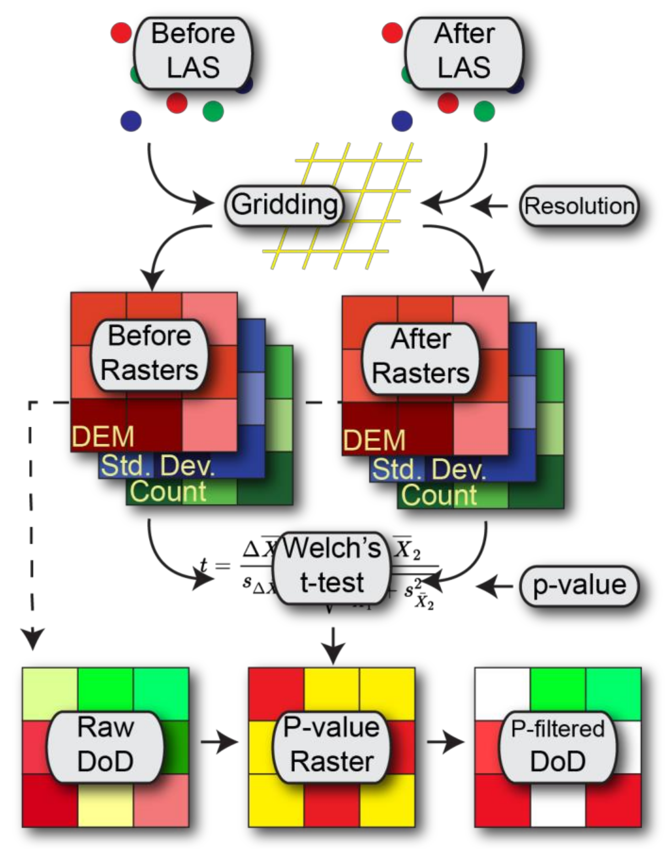
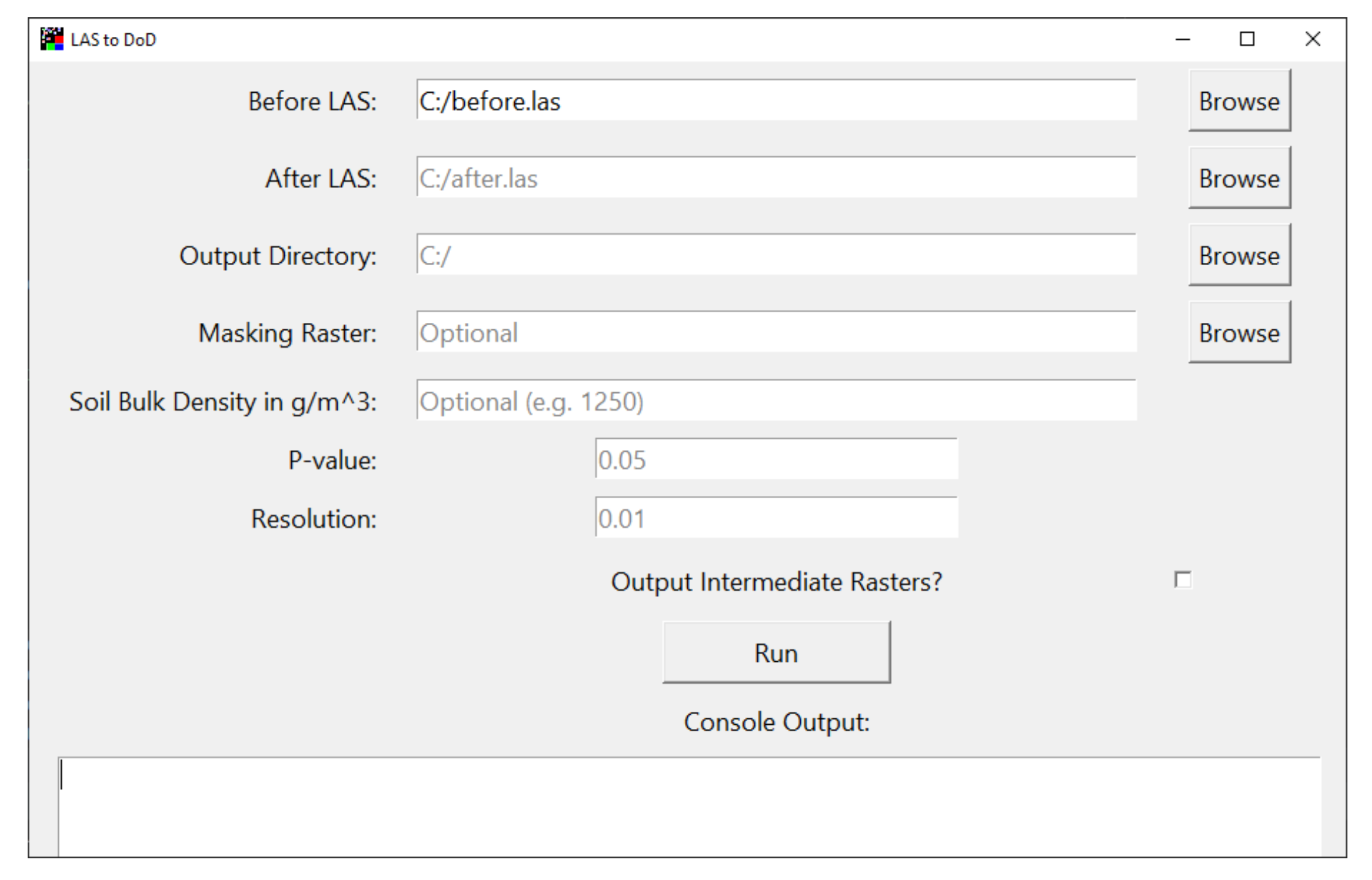
If only considering vertical uncertainty, the true elevation of a DEM cell, Z A c t u a l , can be represented as [33]:
Z A c t u a l = Z D E M   ±   δ z
where Z D E M is the elevation of a DEM cell, and δ z is the elevation uncertainty. Only vertical uncertainty is considered, as horizontal uncertainty, when it is much smaller than the DEM cell size, has little effect on vertical differences in low slope areas [32]. The value of δz can be estimated by different methods, including the standard error from independent check data [8,34,37], the interpolation of vertical standard deviations [7,17], and the root mean square error of data against known control points [30].
The errors inherent to each DEM propagate into the subsequent DoD [38]. The propagated error for the DoD, δ u D o D , can be estimated by [39]:
δ u D o D = δ z n e w 2 + δ z o l d 2
where δ z n e w and δ z o l d represent the uncertainties of the DEMs at two times. This propagated error can be estimated by a minimum level of detection threshold applied to all DEM cells or by a spatially explicit level of detection with a spatial δz estimate. Assuming that δz can be estimated using the standard deviation of error of points within a DEM cell, a probabilistic threshold can be derived using a t-statistic of the two point datasets from the DEM cells at two times [40]:
t = Z D E M n e w Z D E M o l d   δ u D o D
This t-test produces a p-value for each DEM cell, representing the probability of the derived t score on the t-distribution determined by its degrees of freedom. The propagated error, δ u D o D , can be estimated independently based on repeated measurements of the same set of control points, or based on the number of points measured from each cell, assuming the elevation variance of these points represents the uncertainty. In this study, we used the latter assumption because there are typically insufficient repeated measurements of control points to represent a heterogeneous landscape. In contrast, when point clouds are dense compared to the gridding resolution—as they are in TLS or SfM—the points within each grid cell provide sufficient information to estimate the propagated error.
Due to the potential difference in the numbers of points within each DEM cell at the two times, and considering that surfaces can influence the variability in erroneous points, it is highly likely that errors in DEMs used in surface change detection do not have an equal number of points and variance. Therefore, an unequal variance t-test is necessary to determine the confidence interval. The unequal variances t-test is also known as Welch’s t-test [41]. Welch’s t-test is given by:
t = X ¯ 1 X ¯ 2 s 1 2 N 1 + s 2 2 N 2
where X ¯ 1 and X ¯ 2 are the mean point elevations, s 1 and s 2 are the standard deviations, and N 1 and N 2 are numbers of points from each cell of the two DEMs, respectively. The degrees of freedom ( d f ) for the Welch’s t-test is defined as:
d f = s 1 2 N 1 + s 2 2 N 2 2 s 1 4 N 1 2 N 1 1 + s 2 4 N 2 2 N 2 1

2.2. Las2DoD

We developed an algorithm to conduct DoD analysis with spatial varied uncertainty directly based on dense point clouds at two times. Figure 1 illustrates the process flowchart. This algorithm first grids each point cloud based on the specified resolution. The point count (N), mean (X), and standard deviation (s) of the points in each cell are derived for each point cloud. Then, Welch’s t-test is conducted as described above to calculate the t-score for each cell using Equation (4) and derive the p-value based on the t-distribution associated with its degrees of freedom. The p-value is used to determine whether the cell elevation difference is statistically significant at a critical confidence level, such as an alpha level of 0.05 or 95% confidence interval. Finally, a filtered DoD raster is created to show the cells with statistically significant changes. For comparison, the algorithm also generates an unfiltered DoD raster without consideration of uncertainty, a t-score raster, and a p-value raster. The total area and volume changes in erosion and deposition, as well as the net volume change, are also summarized as a text (csv) file.
The above algorithm is coded in Python based on freely available scipy, gdal, and numpy libraries. A standalone user-friendly GUI was also developed to let users specify input point clouds, parameters, and an output folder (Figure 2). Before and after point clouds, a grid resolution, and a target p-value are all that are necessary for this tool to operate. The input point clouds must be in LAS format and are assumed to have approximately the same spatial extent. The X, Y, and Z units of the point clouds must be consistent, and the same units are used for the grid resolution. The input grid resolution is used to determine the grid size for grouping and processing points, as well as the row, column, and resolution of the final rasters. The target p-value will be used as a confidence interval—for example, the target p-value for the 95% confidence level is 0.05—to filter out insignificant results based on the cell-by-cell two-tailed Welch’s t-test. The tool also offers an option to only conduct the DoD analysis to a specific area of interest (AOI) if a masking raster is provided. This masking raster should only contain data within the AOI and use the same unit and coordinate system as the input point clouds. This tool also derives an estimate of the mass of sediment added/removed if an optional soil bulk density is provided. If desired, this tool can also create detailed statistics for each point cloud as raster outputs, such as mean, standard deviation, and point count. The source codes and the executable file for Las2DoD can be found at https://github.com/GeneBailey/Las2DoD (accessed on 20 March 2022).

3. Case Study

We demonstrated the Las2DoD method on a case study to quantify fine-scale soil erosion on two field plots in the southeastern United States. The results were then compared to the DoD analysis with a minimum level of detection ( LoD Min ) and the results from the M3C2 algorithm. The LoD Min and M3C2 methods were selected for comparison due to their frequent appearance in the literature and accessible implementation through available software. With the exception of a single estimate, these two methods are similar to Las2DoD in that they require minimal data preparation and no prior knowledge of elevation uncertainty and related factors.

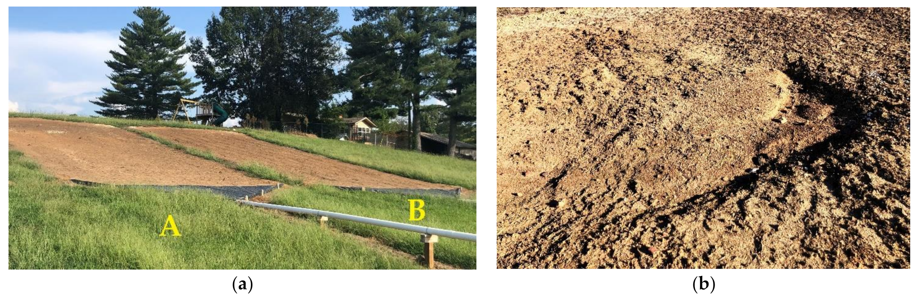
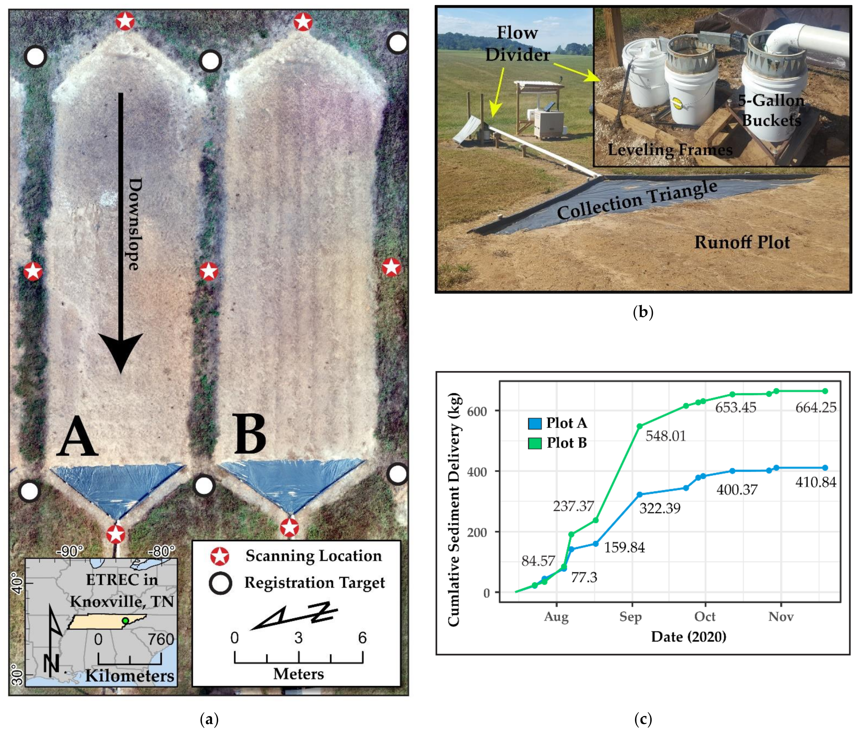
3.1. Study Area and Datasets

Our field site is located at the Plant Science unit of the East Tennessee Research and Education Center (ETREC), University of Tennessee (35.89°, −83.95°) (Figure 3 and Figure 4a). Data were gathered from two experimental plots on the field site. Each plot is approximately 70 m in length, 6 m in width, and on a 15% slope. The plots have been maintained largely free of vegetation through the application of herbicide and the burning of the remaining residue (Figure 3). The plots have different microtopographic features and are not considered replicates. Some rills have developed on the left plot (Plot A) in Figure 4a, especially the one deeply incised rill on the middle-left part (Figure 4b). No rills have developed on the right plot (Plot B), but this plot has some slight ridges running the length of the interior (Figure 4a). These two plots provide the opportunity to test the efficiency of the Las2DoD method to quantify both rill and sheet erosion.
Raised berms were constructed at the sides and top of the plots to control the surface flow. A flow divider system was installed at the bottom of each plot to capture runoff and sediment eroded from the plots (Figure 4b), as used in multiple erosion studies [42,43,44,45]. This flow divider system is designed to capture a precise fraction of up to 3000 gallons of runoff between samplings [46]. Six concrete mounting points were also installed at the corners of each plot as fixed locations for placing registration targets (Figure 4a).
TLS scans were conducted on 6 July 2020 and 19 November 2020. At each date, seven scans were collected by putting the scanner at the top, bottom, and sides of each plot (Figure 4a). All scans were collected using a FARO Focus3D × 330 mounted on a leveled extending tripod. A scanning resolution of half the sensor’s full capability was used to balance the point density and scanning time, producing more than 176 million points over the full field of view for each scan, with an average point spacing of 3 mm at a 10 m distance. The operating time of each scan was roughly 8 min. Using Leica Cyclone software, all TLS point clouds (seven from each date) were registered into a single local coordinate system based on the positions of spherical targets placed on the mounting points at the corners of the plots (Figure 4a). This achieved a positional mean absolute error of 3.5 mm for the final registration. The mean absolute error reported by the Leica Cyclone is defined as an average of the absolute positional distances in the x, y, and z axes between the targets before and after registration [47]. A unified point cloud was then exported for each plot at each scan date. While ground filtering is often a critical step to remove vegetation and other non-ground points when quantifying surface changes from TLS data [48], this study did not apply any ground filtering except for the removal of some noise points far from the plot surface because these well-maintained plots are largely free of vegetation. This practice allowed us to limit the potential smoothing effect of ground-filtering algorithms on surface change detection.
During the study period, sediment was sampled from the flow divider system whenever 2 inches of precipitation occurred at the nearby McGhee Tyson Airport weather station about 11 km away. We sampled the collected sediment 13 times during the study period. The cumulative sediment delivered for plots A and B were 411 kg and 664 kg, respectively (Figure 4c). To enable the estimation of soil mass lost/gained, the soil bulk density of the plots was measured using a nuclear gauge reading the backscatter of the top five centimeters of soil [49,50]. Plot A recorded an average bulk density of 1.25 g/cm3, and Plot B had an average bulk density of 1.39 g/cm3. The volume of change estimations from DoDs can be converted to a net mass change based on these bulk densities. The net mass change estimated from the implemented surface change detection methods can then be compared to the total sediment collected from the flow divider system.

3.2. Change Detection Methods
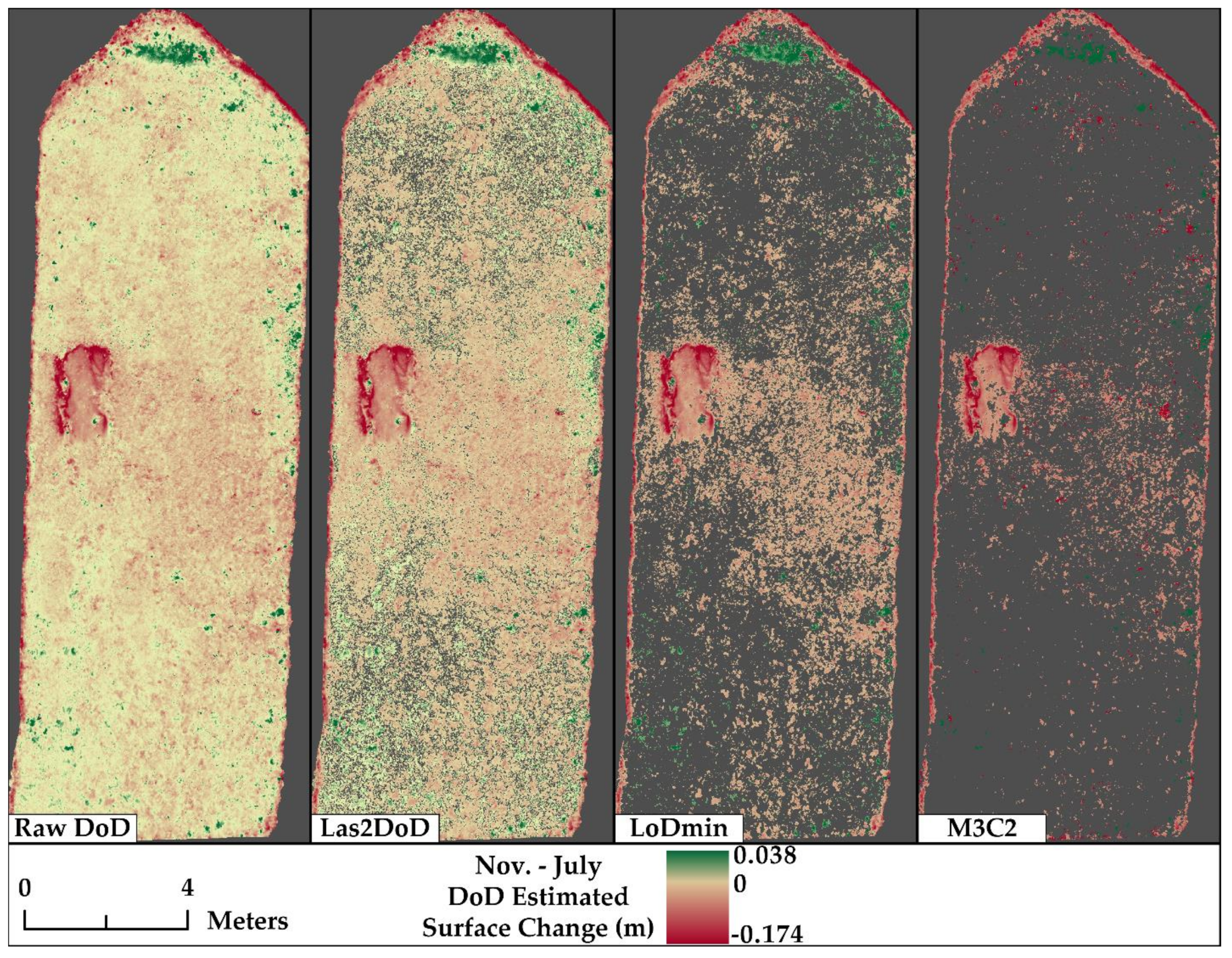
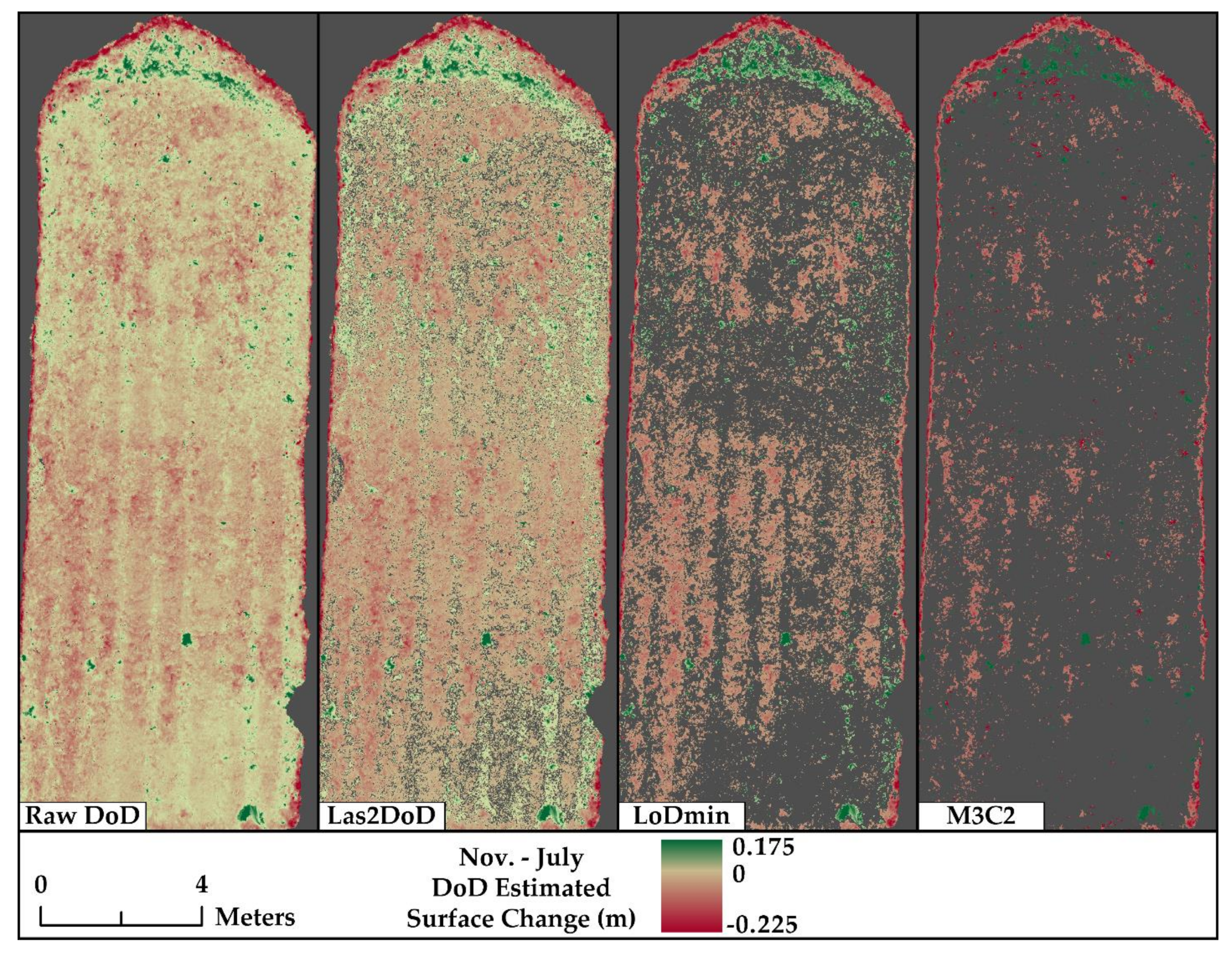
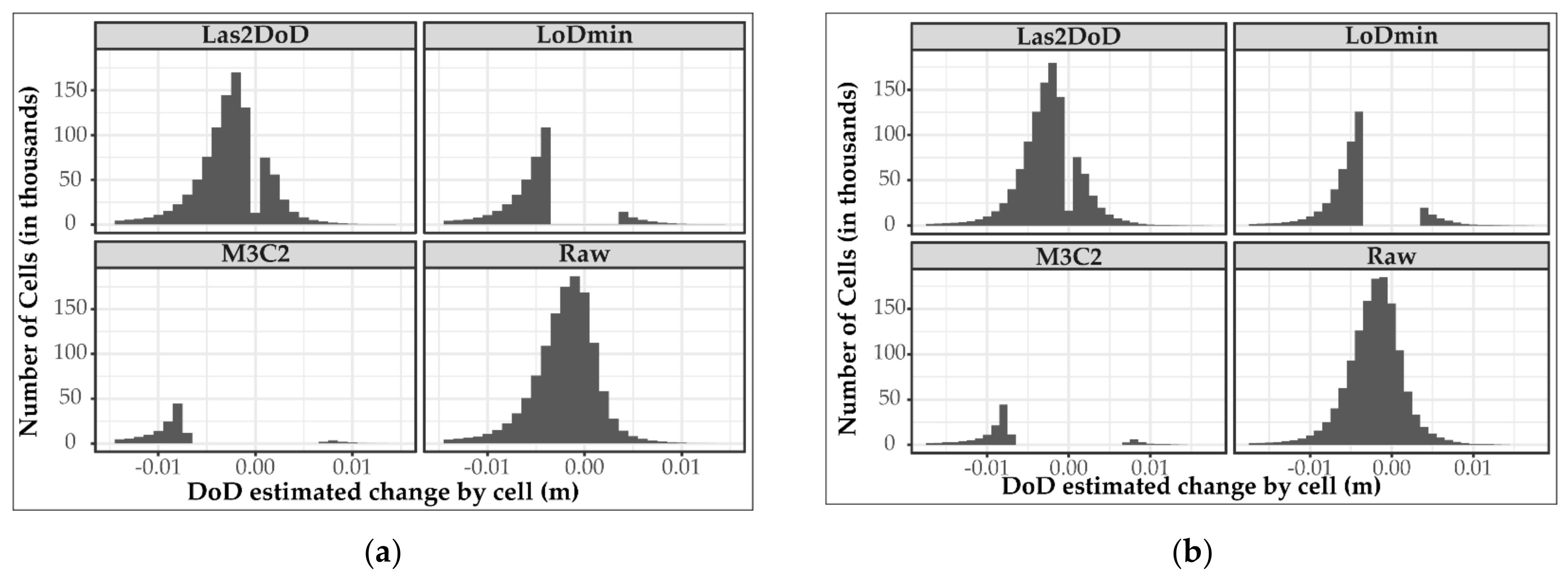
Three methods were used to quantify the topographic changes during the study period. The grid size for the analysis was 1 cm. Studies have suggested that the cell resolution used in the analysis does affect the quantification of surface changes [11]. In our study, a 1 cm resolution provides enough point data within each cell to conduct statistically meaningful analysis while being fine enough not to overgeneralize surface changes. The 1 cm cell size is also much larger than the registered error of point clouds (3.5 mm), limiting the effect of horizontal uncertainty on the DoD analysis [33].
As described in Section 2, Las2DoD requires the input of two point clouds, a target p-value, a cell resolution, and a masking raster. Here, we used the July and November point clouds for each plot, a 0.05 p-value, a cell size of 0.01 m, and a masking raster representing the interior of each plot. The output was compared to the output of the LoD Min and M3C2 methods.
We used the Geomorphic Change Detection software developed by Wheaton et al. [33] to implement the LoD Min method. DEMs for each plot were generated from point clouds from the July and November scans based on the average elevation falling within each 1 cm cell. The DEMs were clipped to only cover the extent of the interior bounds of each plot. In the GCD software, a DoD analysis was performed for each plot using the July and November DEMs and a minimum level of detection threshold of 3.5 mm, corresponding to the point cloud registration error derived from the targets. The resulting DoDs only account for the changes in the cells where the estimated surface change is more than 3.5 mm.
We also used the M3C2 plugin in the open-source CloudCompare software (http://cloudcompare.org/, accessed on 20 March 2022) to conduct point cloud-based change detection analysis. The guidance for this tool suggests that the normal scale parameter is set to a value that is about 25 times the estimated surface roughness at that scale, and the projection scale parameter is large enough that the generated cylinder encompasses on average 20 points while still being small enough to not over-average the distances [31]. For these plots, the values of 0.025 m and 0.01 m for the normals scale and projection scale, respectively, were found to satisfy the recommendations. The normals were calculated using the default settings and operating on every point within the July point clouds. The max depth or height of the cylinder used to identify distance points was set to 2 m to sufficiently include any points. The registration error of 3.5 mm was also included in the uncertainty estimate. The M3C2 generates a point cloud with ‘M3C2 Distance’, ‘Significant Change’, and ‘Distance Uncertainty’ data fields. The points where the distance calculation was not considered significant were filtered from further analysis. M3C2′s distancing estimation operates exclusively on points with various normal directions, and it is hard to directly convert them to volume changes. To enable a comparison to DoD results, the M3C2 output was gridded into 1 cm cells by assigning each cell’s value with the average M3C2 distance of points within the cell. In this way, the M3C2 output can be transformed into a raster format to allow for the calculation of volume changes [24].

3.3. Results

Table 1 and Table 2 list the performance of each method relative to the plot measurements from plots A and B, respectively. For Plot A, among these three methods, Las2DoD estimated 369 kg of mass lost, about 90% of the total 411 kg measured sediment at the bottom of the plot. In comparison, LoD Min and M3C2 estimated 70% and 58% of the total measured sediment, respectively. In comparison, the accuracy of all methods was decreased for Plot B, although a similar pattern exists among the three methods. Las2DoD generated the most accurate estimate and captured 63% of the measured sediment delivery of 664 kg, whereas the LoD Min and M3C2 methods only estimated 48% and 30% of the measured sediment delivery, respectively. In terms of the number of cells with statistically significant changes, the three methods were substantially different. Las2DoD identified 79.5% (Plot A) and 83.7% (Plot B) of the total plot areas to have significant changes, while M3C2 identified only 12.9% and 10.9% and LoD Min 31.1% and 46.07% for these two plots, respectively. For both plots, the methods that reported a greater percentage of cells with significant change also estimated the net mass change more accurately.
Figure 5 and Figure 6 illustrate the spatial distribution of the detectable changes captured by each method alongside a Raw DoD created by simply subtracting DEMs without any consideration of uncertainty. The Raw DoD is included to provide spatial context for the DoD cells excluded through uncertainty testing, but it is not used as a measure of performance. All methods capture the areas of the most extreme change, as can be seen by the areas of deposition at the tops and edges of both plots and the large erosional feature at the middle-left of Plot A. Unsurprisingly, the areas with minimal distance differences are excluded by all methods. In agreement with Table 1 and Table 2, Las2DoD captures more cells of change than the other methods, and a large portion of the captured cells are of lower magnitude changes. In cells where both Las2DoD and LoD Min detect significant changes, the values of the changes are identical. This is not necessarily true for M3C2 because M3C2 calculates distances between the surfaces along the normal direction, whereas Las2DoD and LoD Min strictly measure the vertical distance. This is evidenced by several areas along the right side of Plot A and the top of Plot B, which are identified as strongly erosional in the M3C2 results but are largely absent in other DoDs.
Figure 7 shows the histograms of the DoD results for each plot, highlighting the changes discarded by different methods. The histograms for both plots appear remarkably similar. Without the consideration of uncertainty, the raw DoDs appear to both have a normal distribution around a mean change of −2.3 mm and −2.2 mm for plots A and B. Las2DoD detects less change around zero relative to the raw DoD but still retains some surface changes within ±3.5 mm that are discarded when using the LoD Min and M3C2 methods.

4. Discussion

Compared to the measured plot sediment delivery, Las2DoD produces the most accurate estimates of sediment mass delivery at 90% and 63% for plots A and B, respectively. The performative difference between plots A and B relative to the measured sediment delivery is attributed to the prevalence of sheet erosion on Plot B, which is inherently more challenging to capture. Las2DoD also discerns a greater surface area of change, representing 75% and 83% of the total surface area. This result suggests that Las2DoD can be used in situations where surface change is spread out spatially, but the magnitude of change is at a scale similar to the positional uncertainty of the derived surfaces, as is often the case in areas experiencing interrill erosion. The interrill areas have been found to contribute to as much as 46% of the total erosion on a bare tilled plot with developed rills [51]. It is therefore essential for Las2DoD or other similar methods to account for spatially varied uncertainty and discern minor surface changes in order to capture a total picture of hillslope erosion.
Note that the Las2DoD method ignores registration errors or any errors incorporated into the point cloud before using the method. In performing Welch’s t-test, Las2DoD’s uncertainty analysis can reduce the effect of outliers and noisy points given enough correctly placed points within a cell. When these erroneous points increase the vertical standard deviation of a cell surface such that the difference of means cannot discern a statistically significant difference, the cell will be disregarded. This is not true for methods only considering distance differences, like LoD Min , where if the outlier-affected distance is greater than the threshold, it will be included in the analysis.
The uncertainty analysis will not handle systematic errors within a point cloud, like tilting resulting from an improper registration. While LoD Min and M3C2 are likely over-conservative in accounting for registration errors, obscuring minor surface changes, Las2DoD may capture more erroneous change due to registration error. The registration error observed for this case study (3.5 mm) is based on the deviation of points recorded on registration targets at the corners outside of the area of interest. This error is likely overestimated for most locations in the interior of the plot, as the propagated registration error from targets will increase with increasing distance between individual targets and the barycenter of all targets [47,52]. Although it is not directly accounted for within the Las2DoD method, care must be taken to ensure that the registration of point clouds is as accurate as possible to reduce the impact of systematic errors.
While Las2DoD estimated 90% of the measured sediment delivery for Plot A, it is not an indication that this method always produces this level of accuracy, as highlighted by Plot B. The absolute accuracy results are likely site-specific and related to a combination of local topography, registration, the absence of large vegetation, scan point density, and cell resolution. Accurately measuring small-scale diffuse erosion is a complex task, but the performance of Las2DoD relative to the other studied methods suggests that Las2DoD may positively contribute to the accuracy of DoD estimations. For this case study, Las2DoD includes more cells of minor change to derive more accurate results than the other two methods, which are more conservative due to the inclusion of likely overestimated registration error. The difference between the results of these methods may be reduced on surfaces that experience extreme changes, such as gully erosion and streambank erosion.
Las2DoD only requires a grid resolution and p-value as parameters, both of which can be easily conceptualized and determined. This presents a potential advantage over other, more complex methods like M3C2. While more robust to the influences of local topography, the selection of the suitable parameters for M3C2 can be especially difficult when lacking empirical data to assess the performance of the algorithm under different parameter settings. Therefore, Las2DoD provides an easy and fast way to detect surface changes, and it can be beneficial over other methods where the proper input parameters are unclear or unavailable. In addition, Las2DoD can also generate a set of intermediate rasters, such as the mean and standard deviation rasters of the point cloud, which can be integrated with the Geomorphic Change Detection software or many other terrain analysis software packages for additional analyses.
Las2DoD operates best when the combination of point density and selected grid resolution allow for a high number of points within each cell because it relies on cell-by-cell statistical analysis. The current version of Las2DoD assigns the elevation of each DEM cell as the mean height of the points with the cell to be consistent with Welch’s t-test. The minimum point elevation is occasionally used to inform DEM elevation [6,10]. Many studies also assign an interpolated elevation value using nearest neighbor interpolation [17], bilinear interpolation [11], a triangulated irregular network [8], inverse distance weighting [10], or kriging [16]. Future work is needed to explore the alternate cell height assignments in the Las2DoD analysis. At the same time, the spatial resolution of the specified grid also affects the representation of the surface. Although it is generally believed that finer resolutions provide more precise representations of the surface, finer resolutions also make the final DEM more sensitive to outliers and potentially create more cells with no data [11]. Therefore, more work is necessary to determine the optimal cell resolution for DoD analysis.
While Las2DoD is intended to be used broadly, it is important to note that the case study in this paper represents highly controlled conditions using TLS and its related processing workflow. The controlled nature of the case study limits confounding factors and offers a promising basis to build upon. Further investigation is needed before Las2DoD is recommended to be applied to natural conditions. Future studies may investigate the application of Las2DoD using other sources of high-density points clouds like SfM, explore the performance of the method on different terrains under a variety of conditions, or assess the impact of alternative registration and filtering approaches.

5. Conclusions

This paper presents a straightforward method—Las2DoD—to generate DoDs from point clouds with spatially varied uncertainty. This method uses a specified cell size to derive the mean and standard deviation of the elevations of the points, as well as the point count within each cell of the point clouds collected at different times. These derived datasets are then applied in a Welch’s t-test to test whether each cell has a significant difference in mean elevation based on a specified confidence level. The results from the t-test are used to filter cells with insignificant changes. The whole process is coded in Python with a standalone GUI.
This proposed method was applied to a case study using TLS point clouds to quantify mixed rill–interrill erosion on natural rainfall hillslope erosion plots and compared the results with the results estimated by a minimum level of detection filtered DoD and a DoD summarized from the M3C2 algorithm. The results of these methods are also compared with the measured sediment delivery from the plots to assess the performance of each method. Our results indicate Las2DoD has the best performance with an estimation of 90% of the measured sediment on the plot with rill erosion, whereas the other two methods estimated 70% and 58% of the total measured sediment, respectively. For the plot dominated by sheet erosion, the absolute accuracy of all methods was reduced, but the performance pattern between the methods was highly similar. Both plots demonstrate that Las2DoD captures more low-magnitude topographic change, while the other methods are more conservative and only capture relatively high-magnitude changes.
Las2DoD offers a simple and straightforward way to implement DoD analysis with spatial varied uncertainty. It provides a fast and easy way to detect surface changes and quantify erosion and deposition, as well as the net volume changes of a surface. This method only requires the dense point clouds and easily conceptualized and determined cell size and confidence level, without additional information or extensive parameterization. It may be particularly useful when other DoD methods may be over-conservative, and the change experienced on a large portion of the surface is of low magnitude but may contribute to a significant portion to change in elevation, such as the interrill erosion of hillslopes.

Author Contributions

Conceptualization, G.B. and Y.L.; funding acquisition, G.B., Y.L. and R.W.-A.; investigation, G.B., Y.L., N.M., D.Y. and W.W.; methodology, G.B., Y.L., N.M. and D.Y.; project administration, Y.L. and R.W.-A.; resources, Y.L., N.M., D.Y. and W.W.; software, G.B.; visualization, G.B.; writing—original draft, G.B.; writing—review and editing, Y.L., N.M., D.Y., W.W. and R.W.-A. All authors have read and agreed to the published version of the manuscript.

Funding

This research received financial support from the Environmental Protection Agency Small Urban Water Grant (UW-00D45316) to Y.L. and R.W.-A., the Carole Anne Shirley Memorial Fund to Y.L., and the Stewart K. McCroskey Memorial Fund to G.B. from the Department of Geography, University of Tennessee, and the start-up fund to R.W.-A. from the University of Nevada, Reno. Funding for open access to this research was provided by the University of Tennessee’s Open Publishing Support Fund.

Institutional Review Board Statement

Not applicable.

Informed Consent Statement

Not applicable.

Data Availability Statement

The data related to this study are available on request from the authors. The Las2DoD code can be found at https://github.com/GeneBailey/Las2DoD (accessed on 20 March 2022).

Acknowledgments

The authors thank Yasin Wahid Rabby and Ming Shen for the help in the field surveys. Hannah Herrero and Nicholas Nagle are also acknowledged for comments on early drafts.

Conflicts of Interest

The authors declare no conflict of interest. The funders had no role in the design of the study; in the collection, analyses, or interpretation of data; in the writing of the manuscript, or in the decision to publish the results.

References

  1. Lefsky, M.A.; Cohen, W.B.; Parker, G.G.; Harding, D.J. Lidar Remote Sensing for Ecosystem StudiesLidar, an Emerging Remote Sensing Technology That Directly Measures the Three-Dimensional Distribution of Plant Canopies, Can Accurately Estimate Vegetation Structural Attributes and Should Be of Particular Interest to Forest, Landscape, and Global Ecologists. BioScience 2002, 52, 19–30. [Google Scholar] [CrossRef]
  2. Tarolli, P. High-Resolution Topography for Understanding Earth Surface Processes: Opportunities and Challenges. Geomorphology 2014, 216, 295–312. [Google Scholar] [CrossRef]
  3. Tarolli, P.; Dalla Fontana, G. Hillslope-to-Valley Transition Morphology: New Opportunities from High Resolution DTMs. Geomorphology 2009, 113, 47–56. [Google Scholar] [CrossRef]
  4. Slatton, K.C.; Carter, W.E.; Shrestha, R.L.; Dietrich, W. Airborne Laser Swath Mapping: Achieving the Resolution and Accuracy Required for Geosurficial Research. Geophys. Res. Lett. 2007, 34, L23S10. [Google Scholar] [CrossRef]
  5. Perroy, R.L.; Bookhagen, B.; Asner, G.P.; Chadwick, O.A. Comparison of Gully Erosion Estimates Using Airborne and Ground-Based LiDAR on Santa Cruz Island, California. Geomorphology 2010, 118, 288–300. [Google Scholar] [CrossRef]
  6. Höfle, B.; Griesbaum, L.; Forbriger, M. GIS-Based Detection of Gullies in Terrestrial LiDAR Data of the Cerro Llamoca Peatland (Peru). Remote Sens. 2013, 5, 5851–5870. [Google Scholar] [CrossRef] [Green Version]
  7. Li, Y.; McNelis, J.J.; Washington-Allen, R.A. Quantifying Short-Term Erosion and Deposition in an Active Gully Using Terrestrial Laser Scanning: A Case Study From West Tennessee, USA. Front. Earth Sci. 2020, 8, 14. [Google Scholar] [CrossRef]
  8. Goodwin, N.R.; Armston, J.D.; Muir, J.; Stiller, I. Monitoring Gully Change: A Comparison of Airborne and Terrestrial Laser Scanning Using a Case Study from Aratula, Queensland. Geomorphology 2017, 282, 195–208. [Google Scholar] [CrossRef]
  9. Rengers, F.K.; Tucker, G.E. The Evolution of Gully Headcut Morphology: A Case Study Using Terrestrial Laser Scanning and Hydrological Monitoring. Earth Surf. Process. Landf. 2015, 40, 1304–1317. [Google Scholar] [CrossRef]
  10. Eltner, A.; Baumgart, P. Accuracy Constraints of Terrestrial Lidar Data for Soil Erosion Measurement: Application to a Mediterranean Field Plot. Geomorphology 2015, 245, 243–254. [Google Scholar] [CrossRef]
  11. Lu, X.; Li, Y.; Washington-Allen, R.A.; Li, Y.; Li, H.; Hu, Q. The Effect of Grid Size on the Quantification of Erosion, Deposition, and Rill Network. Int. Soil Water Conserv. Res. 2017, 5, 241–251. [Google Scholar] [CrossRef]
  12. Lu, X.; Li, Y.; Washington-Allen, R.A.; Li, Y. Structural and Sedimentological Connectivity on a Rilled Hillslope. Sci. Total Environ. 2019, 655, 1479–1494. [Google Scholar] [CrossRef] [PubMed]
  13. Li, Y.; Lu, X.; Washington-Allen, R.A.; Li, Y. Microtopographic Controls on Erosion and Deposition of a Rilled Hillslope in Eastern Tennessee, USA. Remote Sens. 2022, 14, 1315. [Google Scholar] [CrossRef]
  14. Day, S.S.; Gran, K.B.; Belmont, P.; Wawrzyniec, T. Measuring Bluff Erosion Part 1: Terrestrial Laser Scanning Methods for Change Detection. Earth Surf. Process. Landf. 2013, 38, 1055–1067. [Google Scholar] [CrossRef]
  15. Vericat, D.; Smith, M.W.; Brasington, J. Patterns of Topographic Change in Sub-Humid Badlands Determined by High Resolution Multi-Temporal Topographic Surveys. CATENA 2014, 120, 164–176. [Google Scholar] [CrossRef]
  16. Schürch, P.; Densmore, A.L.; Rosser, N.J.; Lim, M.; McArdell, B.W. Detection of Surface Change in Complex Topography Using Terrestrial Laser Scanning: Application to the Illgraben Debris-Flow Channel. Earth Surf. Process. Landf. 2011, 36, 1847–1859. [Google Scholar] [CrossRef]
  17. Cândido, B.M.; Quinton, J.N.; James, M.R.; Silva, M.L.N.; de Carvalho, T.S.; de Lima, W.; Beniaich, A.; Eltner, A. High-Resolution Monitoring of Diffuse (Sheet or Interrill) Erosion Using Structure-from-Motion. Geoderma 2020, 375, 114477. [Google Scholar] [CrossRef]
  18. Bolkas, D.; Naberezny, B.; Jacobson, M.G. Comparison of SUAS Photogrammetry and TLS for Detecting Changes in Soil Surface Elevations Following Deep Tillage. J. Surv. Eng. 2021, 147, 04021001. [Google Scholar] [CrossRef]
  19. Meijer, A.D.; Heitman, J.L.; White, J.G.; Austin, R.E. Measuring Erosion in Long-Term Tillage Plots Using Ground-Based Lidar. Soil Tillage Res. 2013, 126, 1–10. [Google Scholar] [CrossRef]
  20. Turunen, M.; Turtola, E.; Vaaja, M.T.; Hyväluoma, J.; Koivusalo, H. Terrestrial Laser Scanning Data Combined with 3D Hydrological Modeling Decipher the Role of Tillage in Field Water Balance and Runoff Generation. CATENA 2020, 187, 104363. [Google Scholar] [CrossRef]
  21. Westoby, M.J.; Brasington, J.; Glasser, N.F.; Hambrey, M.J.; Reynolds, J.M. ‘Structure-from-Motion’ Photogrammetry: A Low-Cost, Effective Tool for Geoscience Applications. Geomorphology 2012, 179, 300–314. [Google Scholar] [CrossRef] [Green Version]
  22. James, M.R.; Robson, S. Straightforward Reconstruction of 3D Surfaces and Topography with a Camera: Accuracy and Geoscience Application. J. Geophys. Res. Earth Surf. 2012, 117, 03017. [Google Scholar] [CrossRef] [Green Version]
  23. Prosdocimi, M.; Calligaro, S.; Sofia, G.; Dalla Fontana, G.; Tarolli, P. Bank Erosion in Agricultural Drainage Networks: New Challenges from Structure-from-Motion Photogrammetry for Post-Event Analysis. Earth Surf. Process. Landf. 2015, 40, 1891–1906. [Google Scholar] [CrossRef]
  24. Meinen, B.U.; Robinson, D.T. Where Did the Soil Go? Quantifying One Year of Soil Erosion on a Steep Tile-Drained Agricultural Field. Sci. Total Environ. 2020, 729, 138320. [Google Scholar] [CrossRef]
  25. Kaiser, A.; Erhardt, A.; Eltner, A. Addressing Uncertainties in Interpreting Soil Surface Changes by Multitemporal High-Resolution Topography Data across Scales. Land Degrad. Dev. 2018, 29, 2264–2277. [Google Scholar] [CrossRef]
  26. Neugirg, F.; Stark, M.; Kaiser, A.; Vlacilova, M.; Della Seta, M.; Vergari, F.; Schmidt, J.; Becht, M.; Haas, F. Erosion Processes in Calanchi in the Upper Orcia Valley, Southern Tuscany, Italy Based on Multitemporal High-Resolution Terrestrial LiDAR and UAV Surveys. Geomorphology 2016, 269, 8–22. [Google Scholar] [CrossRef]
  27. Whitehead, K.; Moorman, B.J.; Hugenholtz, C.H. Brief Communication: Low-Cost, on-Demand Aerial Photogrammetry for Glaciological Measurement. Cryosphere 2013, 7, 1879. [Google Scholar] [CrossRef] [Green Version]
  28. Cook, K.L. An Evaluation of the Effectiveness of Low-Cost UAVs and Structure from Motion for Geomorphic Change Detection. Geomorphology 2017, 278, 195–208. [Google Scholar] [CrossRef]
  29. Girardeau-Montaut, D.; Roux, M.; Marc, R.; Thibault, G. Change Detection on Point Cloud Data Acquired with a Ground Laser Scanner. Int. Arch. Photogramm. Remote Sens. Spat. Inf. Sci. 2005, 36, W19. [Google Scholar]
  30. Nourbakhshbeidokhti, S.; Kinoshita, A.; Chin, A.; Florsheim, J. A Workflow to Estimate Topographic and Volumetric Changes and Errors in Channel Sedimentation after Disturbance. Remote Sens. 2019, 11, 586. [Google Scholar] [CrossRef] [Green Version]
  31. Lague, D.; Brodu, N.; Leroux, J. Accurate 3D Comparison of Complex Topography with Terrestrial Laser Scanner: Application to the Rangitikei Canyon (N-Z). ISPRS J. Photogramm. Remote Sens. 2013, 82, 10–26. [Google Scholar] [CrossRef] [Green Version]
  32. Williams, R. DEMs of Difference. Geomorphol. Tech. 2012, 2, 1–17. [Google Scholar]
  33. Wheaton, J.M.; Brasington, J.; Darby, S.E.; Sear, D.A. Accounting for uncertainty in DEMs from repeat topographic surveys: Improved sediment budgets. Earth Surf. Process. Landf. 2010, 35, 136–156. [Google Scholar] [CrossRef]
  34. Brasington, J.; Rumsby, B.T.; McVey, R.A. Monitoring and modelling morphological change in a braided gravel-bed river using high resolution GPS-based survey. Earth Surf. Process. Landf. 2000, 25, 973–990. [Google Scholar] [CrossRef]
  35. Wheaton, J.M. Uncertainty in Morphological Sediment Budgeting of Rivers. Ph.D. Thesis, University of Southampton, Southampton, UK, 2008. [Google Scholar]
  36. Blasone, G.; Cavalli, M.; Marchi, L.; Cazorzi, F. Monitoring Sediment Source Areas in a Debris-Flow Catchment Using Terrestrial Laser Scanning. CATENA 2014, 123, 23–36. [Google Scholar] [CrossRef]
  37. Croke, J.; Todd, P.; Thompson, C.; Watson, F.; Denham, R.; Khanal, G. The Use of Multi Temporal LiDAR to Assess Basin-Scale Erosion and Deposition Following the Catastrophic January 2011 Lockyer Flood, SE Queensland, Australia. Geomorphology 2013, 184, 111–126. [Google Scholar] [CrossRef]
  38. James, L.A.; Hodgson, M.E.; Ghoshal, S.; Latiolais, M.M. Geomorphic Change Detection Using Historic Maps and DEM Differencing: The Temporal Dimension of Geospatial Analysis. Geomorphology 2012, 137, 181–198. [Google Scholar] [CrossRef]
  39. Brasington, J.; Langham, J.; Rumsby, B. Methodological Sensitivity of Morphometric Estimates of Coarse Fluvial Sediment Transport. Geomorphology 2003, 53, 299–316. [Google Scholar] [CrossRef]
  40. Lane, S.N.; Westaway, R.M.; Hicks, D.M. Estimation of erosion and deposition volumes in a large, gravel-bed, braided river using synoptic remote sensing. Earth Surf. Process. Landf. 2003, 28, 249–271. [Google Scholar] [CrossRef]
  41. Welch, B.L. The Generalization of `Student’s’ Problem When Several Different Population Variances Are Involved. Biometrika 1947, 34, 28–35. [Google Scholar] [CrossRef]
  42. Bonilla, C.A.; Kroll, D.G.; Norman, J.M.; Yoder, D.C. Instrumentation for Measuring Runoff, Sediment, and Chemical Losses from Agricultural Fields. J. Environ. Qual. 2006, 35, 216–223. [Google Scholar] [CrossRef] [Green Version]
  43. Hoomehr, S.; Schwartz, J.S.; Yoder, D.C.; Drumm, E.C.; Wright, W. Curve Numbers for Low-Compaction Steep-Sloped Reclaimed Mine Lands in the Southern Appalachians. J. Hydrol. Eng. 2013, 18, 1627–1638. [Google Scholar] [CrossRef]
  44. Seo, Y.; Lee, J.; Hart, W.E.; Denton, H.P.; Yoder, D.C.; Essington, M.E.; Perfect, E. SEDIMENT LOSS AND NUTRIENT RUNOFF FROM THREE FERTILIZER APPLICATION METHODS. Trans. ASAE 2005, 48, 2155–2162. [Google Scholar] [CrossRef]
  45. Yoder, D.C.; Cope, T.L.; Wills, J.B.; Denton, H.P. No-till Transplanting of Vegetables and Tobacco to Reduce Erosion and Nutrient Surface Runoff. J. Soil Water Conserv. 2005, 60, 68–73. [Google Scholar]
  46. Pinson, W.T.; Yoder, D.C.; Buchanan, J.R.; Wright, W.C.; Wilkerson, J.B. Design and evaluation of an improved flow divider for sampling runoff plots. Appl. Eng. Agric. 2004, 20, 433. [Google Scholar] [CrossRef]
  47. Fan, L.; Smethurst, J.A.; Atkinson, P.M.; Powrie, W. Error in Target-Based Georeferencing and Registration in Terrestrial Laser Scanning. Comput. Geosci. 2015, 83, 54–64. [Google Scholar] [CrossRef] [Green Version]
  48. Barneveld, R.J.; Seeger, M.; Maalen-Johansen, I. Assessment of Terrestrial Laser Scanning Technology for Obtaining High-Resolution DEMs of Soils: TLS FOR HIGH-RESOLUTION DEMS. Earth Surf. Process. Landf. 2013, 38, 90–94. [Google Scholar] [CrossRef]
  49. Randrup, T.; Lichter, J. Measuring Soil Compaction on Construction Sites: A Review of Surface Nuclear Gauges and Penetrometers. J. Arboric. 2001, 27, 109–117. [Google Scholar] [CrossRef]
  50. Rousseva, S.S.; Ahuja, L.R.; Heathman, G.C. Use of a Surface Gamma-Neutron Gauge for in Situ Measurement of Changes in Bulk Density of the Tilled Zone. Soil Tillage Res. 1988, 12, 235–251. [Google Scholar] [CrossRef]
  51. Govers, G.; Poesen, J. Assessment of the Interrill and Rill Contributions to Total Soil Loss from an Upland Field Plot. Geomorphology 1988, 1, 343–354. [Google Scholar] [CrossRef]
  52. Yang, R.; Meng, X.; Yao, Y.; Chen, B.Y.; You, Y.; Xiang, Z. An Analytical Approach to Evaluate Point Cloud Registration Error Utilizing Targets. ISPRS J. Photogramm. Remote Sens. 2018, 143, 48–56. [Google Scholar] [CrossRef]
Figure 1. Flowchart showing an overview of the Las2DoD process.
Remotesensing 14 01537 g001
Figure 2. Las2DoD GUI interface.
Remotesensing 14 01537 g002
Figure 3. (a) Photograph of study site from the bottom of the slope. Plots A and B are indicated. (b) Close photo of Plot A soil surface.
Remotesensing 14 01537 g003
Figure 4. (a) East Tennessee Research and Education Center (ETREC) study site with plots A and B used in the case study. (b) Photograph showing the flow divider system on plot B. (c) Cumulative sediment delivery data sampled from the field plots.
Remotesensing 14 01537 g004
Figure 5. DoD results from Plot A of a DoD without uncertainty analysis and the three tested methods with uncertainty testing.
Remotesensing 14 01537 g005
Figure 6. DoD results from Plot B of a DoD without uncertainty analysis and the three tested methods with uncertainty testing.
Remotesensing 14 01537 g006
Figure 7. Histograms from the final DoD of the selected uncertainty analysis methods and a raw DoD without uncertainty analysis for Plot A (a) and Plot B (b).
Remotesensing 14 01537 g007
Table 1. Results from applying the three change detection methods in comparison with the plot measurements for Plot A.
MethodArea of Significant Change (m2)Percentage of Surface Represented (%)Volume Added (m3)Volume Removed (m3)Total Volume Change (m3)Estimated Mass Change (kg) 1Estimated Mass Change/Measured Sediment Delivery 2
Las2DoD101.6579.50.050.34−0.30−3690.90
M3C216.4812.90.010.2−0.19−2370.58
LoD Min 39.7431.10.020.25−0.23−287.50.70
1 Estimated mass change is equal to the total volume change multiplied by the plot’s soil bulk density of 1.25 g/cm3. 2 The measured sediment delivery of Plot A is 411 kg.
Table 2. Results from applying the three change detection methods in comparison with the plot measurements for Plot B.
MethodArea of Significant Change (m2)Percentage of Surface Represented (%)Volume Added (m3)Volume Removed (m3)Total Volume Change (m3)Estimated Mass Change (kg) 1Estimated Mass Change/Measured Sediment Delivery 2
Las2DoD112.3683.70.060.36−0.30−4160.63
M3C214.6810.90.020.16−0.14−1980.30
LoD Min 46.0734.30.030.26−0.23−3200.48
1 Estimated mass change is equal to the total volume change multiplied by the plot’s soil bulk density of 1.39 g/cm3. 2 The measured sediment delivery of Plot B is 664 kg.
Publisher’s Note: MDPI stays neutral with regard to jurisdictional claims in published maps and institutional affiliations.

