Wavefield Reconstruction Inversion Based on the Multi-Scale Cumulative Frequency Strategy for Ground-Penetrating Radar Data: Application to Urban Underground Pipeline

Abstract

High-precision detection of the underground pipelines is an indispensable part of the development and construction of cities. At present, the inversion technology for ground-penetrating radar (GPR) data is an effective means of realizing shallow-underground-space visualization in the field of geophysical exploration. However, the traditional full-waveform inversion (FWI) method usually faces the problems of strong nonlinearity of the objective function, high dependence on the initial model, and huge calculation cost. For improving the accuracy and efficiency of GPR data inversion, a wavefield reconstruction inversion (WRI) strategy is used for GPR data imaging to reduce the nonlinearity of the inversion problem and the dependence on the initial model. Then, the frequency weighting strategy and the multi-scale method are adopted to avoid the high-frequency component data dominating the optimization process and enhance the stability of inversion. In this paper, two numerical experiments of pipeline models with different materials and spacing or buried depths verified that the proposed method can effectively reconstruct the subsurface pipelines, and further performance of our algorithm on the field data verified the reliability of high-precision imaging of urban underground pipelines, which shows great potential of application in the field of high-precision detection of the urban underground pipelines.

1. Introduction

Accurate and high-precision detection of urban underground pipelines, which is a necessary measure to ensure the urban construction, has achieved a pivotal position in the management and development of urban underground space [1]. Among the shallow detection methods, ground-penetrating radar (GPR) nondestructive detection technology plays an important role in urban exploration [1,2,3,4]. It has the potential for the reconstruction of the subsurface structures, and the relative imaging studies have been concerned with the location [5], the classification [6], and the estimation of size and infilling material [7] of the buried objects for urban detection. The studies regarding the algorithm improvement of inversion for the on-ground GPR data [8,9,10,11] and the borehole radar data [12,13] are of great significance for quickly and accurately obtaining the professional information of pipes, such as the location, depth, diameter, material, etc.

The anticipate objective of the imaging for on-ground GPR data is to accurately locate and qualitatively describe the underground targets by rationally utilizing the collected data within a limited time until realizing the visualization [14]. Among the geophysical imaging methods, full-waveform inversion (FWI), which is a high-resolution technology, has been widely studied and rapidly developed in recent years. At present, FWI of GPR data has become an effective means to quantitatively characterize the parameters’ distribution of shallow underground media [15,16,17]. When performing the inversion for GPR data, it is firstly considered that frequency-domain inversion has great advantages in calculation time from the aspect of calculation domain. That is, by inverting a small amount of frequency component data, inversion in the frequency domain can not only avoid the data redundancy in inverting all frequency components, but also can achieve a result consistent with that in the time domain [15,18], thereby saving the calculation cost [19]. Additionally, the frequency-domain inversion strategy has a natural multi-scale characteristic. That is, by adopting appropriate frequency strategy, inversion in the frequency domain can quickly and easily realize the inversion result similar to that of time-domain multi-scale strategy [20], thereby effectively avoiding the inversion result falling into local minimum and reducing the influence of nonlinearity of the inversion problem. Therefore, in this paper, we mainly focus on the frequency-domain inversion method for on-ground GPR data. In the initial studies of the GPR inversion in the frequency domain, only single-parameter inversion of permittivity model [16,21] or dual-parameter imaging [22,23] of simple layered media has been realized; later, it was developed into dual-parameter simultaneous inversion using a parameter scaling strategy [15,24] or a cross gradient strategy [17], and the accuracy of the model reconstruction was improved. For the selection of frequency strategy, it was noted that although the sequential inversion strategy of finite frequency components can reduce the nonlinear problems such as cycle skipping [17], it cannot perform parallel calculation, and the computation efficiency is limited. Another relatively efficient multi-frequency simultaneous inversion strategy calculates all the selected frequency components at the same time, which, however, often leads to the dominant role of high-frequency data components, making it difficult to recover the background structural information, easily affected by cycle skipping, and strongly dependent on the initial model [24]. Fortunately, (a) the simultaneous multi-frequency weighting strategy and (b) the cumulative sequential strategy can solve the above problems. For the first method, if each frequency component is properly weighted, it can avoid the high-frequency component data dominating the optimization process. Watson [16] compared the FWI results under the conditions with equal or different weights of frequency components and proved that the reasonable weighting factors can “smooth” the oscillation distribution caused by noise and eliminate the artifacts under the greater contrasted object in the inversion results. For the second method, as suggested by Bunks et al. [25] for seismic in the time domain, if we keep the low-frequency data as we move to high frequencies, it can reduce the inversion nonlinearity to a certain extent [24]. This gives us a sense of the importance about the choice of the frequency strategy in the inversion. Up to now, the reliability and feasibility of quantitative imaging for on-ground GPR data have been verified [15,16,26]. However, the traditional FWI is highly nonlinear, highly dependent on the initial model, and has a high computational cost. Therefore, it is necessary to develop a GPR inversion imaging method that can make full use of both the recorded data information and the computing resources.

In our previous work on GPR imaging using wavefield reconstruction inversion (WRI) [14], we found that the selection of the penalty factor and the frequency strategy is critical for the success of inversion. As an improved FWI method, the WRI strategy inverts the wavefields and model parameters at the same time, adds the wave equation as a penalty term to the misfit function, and adjusts the weight of data residual term and wave equation term in the misfit function through the penalty factor. Thereby, it breaks through the nonlinear bottleneck and reduces the dependence on the initial model of traditional full-waveform inversion [27,28,29]. Since WRI was proposed, many scholars have paid attention to its special inversion characteristics, and it has been widely used in seismic inversion; thus, its theoretical framework has also been improved and expanded. In 2013, van Leeuwen and Herrmann [27] optimized the relevant theory of WRI, gave the physical meaning of reconstructed wavefield in frequency domain, and analyzed the influence of penalty factor on inversion. Then, van Leeuwen and Herrmann [28] summed up the influence of penalty factor on inversion results through numerical experiments, and gave the selection strategy. Fang [30] compared the differences between FWI and WRI in detail in his doctoral thesis and conducted relevant model tests. Da Silva and Yao [31] proposed a WRI based on a penalty cost function, which adaptively selects penalty factors, providing a framework for the automatic application of WRI. Aghamiry et al. [32,33,34] used the alternating direction multiplier method to solve the WRI problem and discussed the influence of various media and different regularization methods on the inversion effect. Rizzuti et al. [35] extended WRI from the frequency domain to the time domain and implemented a large-scale three-dimensional inversion problem using dual formula. In 2021, Feng et al. [14] introduced a WRI algorithm into the multi-parameters inversion of on-ground GPR data in the frequency domain, which obtained better inversion results by using simultaneous multi-frequency weighting strategy.

This paper aims to propose a WRI method based on the multi-scale cumulative frequency strategy to invert the subsurface distribution of pipelines. In view of the advantages of WRI in the nonlinearity problem and the sensitivity of the initial model, we consider using WRI to perform the inversion of GPR data for urban underground pipelines. Meanwhile, for improving the applicability and stability of the algorithm and to better reconstruct the distribution of underground media, a variable projection algorithm is used to reconstruct the wavefield. In addition, considering the importance of the selection of the frequency strategy in the frequency-domain inversion algorithm, this paper integrates the idea of cumulative sequential strategy and simultaneous multi-frequency weighting strategy.

The framework of this paper is as follows: in the methods section, regarding forward and inverse problem in the frequency domain for GPR, we firstly introduce the two-dimensional finite-element frequency domain forward equation of GPR wave, then deduce the misfit function of frequency-domain WRI in detail, give the core steps of solving WRI problem by the variable projection method, and explain the technical details of multi-scale cumulative frequency strategy. In the numerical example section, we perform two groups of numerical experiments, of which one is the parallel pipelines model with different materials and another is the pipelines model with different spacings and buried depths; further application is performed by the proposed strategy in a physical pipelines model with field data. Finally, in the discussion and conclusion section, we summarize the relevant conclusions of our proposed inversion method for on-ground GPR data and point out its application prospects and limitations.

2. Forward and Inverse Problem in the Frequency Domain

In this section, we first review the GPR wave equation in the frequency domain. Then, we formulate the WRI problem for permittivity and conductivity and detail the algorithm and strategy used for its solution.

2.1. GPR Finite-Element Frequency Domain Simulation

The governing equation describing the transverse magnetic mode of electromagnetic wave propagation in the frequency domain is given by the following equation [36]:

$$\frac{\partial }{\partial x}\left({\alpha }_x\frac{\partial u}{\partial x}\right)+\frac{\partial }{\partial y}\left({\alpha }_y\frac{\partial u}{\partial y}\right)+\beta k^{2}u=i\omega \mu J_z,$$

(1)

where u (V/m) is the electric field intensity in the frequency domain, J_z (A/m²) is the current density of frequency domain, k is the wavenumber in the frequency domain, and k² = μꞷ²(ε − iσ/ꞷ); here, ꞷ = 2πf is the angular frequency, i = sqrt(−1) is an imaginary unit, and μ (H/m), ε (F/m), and σ (S/m) represent the magnetic conductivity, the permittivity, and the conductivity, respectively. α_x, α_y, and β indicate the relevant parameters introduced for convenience to load the absorbing boundary condition (perfectly matching layers [37] are used in the truncated boundary).

After discretization by the finite-element frequency domain method, the above formula can be written in the matrix form as

$$A\left(\omega ,\epsilon ,\sigma \right)u\left(\omega \right)=q\left(\omega \right),$$

(2)

where A is the Helmholtz operator of partial differential equation (PDE), u is the wavefield vector, and q is the source vector.

2.2. GPR Frequency-Domain WRI

2.2.1. Construction of WRI Misfit Function

In the inversion problem for GPR, the observed data are used to infer the parameters of the underground media that refer to the permittivity and to the conductivity. The traditional FWI problem can be written as a PDE-constrained optimization problem about model parameters, while the WRI replaces the PDE constraint by a penalty term and optimizes for both wavefields and parameters by solving the following unconstrained problem:

$$\underset{u,m}{\min }\frac{1}{2}{‖Pu-d‖}_2^2+\frac{1}{2}{\lambda }^2{‖A(m)u-q‖}_2^2,$$

(3)

where m is the model vector with the size of 2 × N_M, containing both permittivity and conductivity values at each element of the finite-element mesh; here, N_M is the number of the discrete elements, P is a projection operator that restricts the wavefields to the receiver positions, d is the observed GPR data, λ is the penalty parameter, and q is the source vector.

The parameter λ is a penalty scalar, which can balance the misfits between the data term and wave equation term. If λ increases, the wave equation term is more tightly constrained, and the WRI problem will converge to the conventional FWI method. Thereby, the conventional FWI can be regarded as a special case of WRI. In another way, if λ decreases, WRI will expand the search space of the optimization problem by relaxing the constraint of the wave equation [31], so as to mitigate the inversion nonlinearity accordingly, make the inversion contain less local minima, and result in a more accurate reconstruction than the FWI method [16,27,29,30].

For the multi-frequency GPR data inversion, we insert a weighting factor into the WRI misfit function, expressed as

$$\begin{array}{l}\Phi \left(u,m\right)=\frac{1}{2}{\displaystyle \sum _{i=1}^{N_{\omega }}{\displaystyle \sum _{j=1}^{N_s}{\eta }_i{\left(P{u}_{i,j}-d_{i,j}\right)}^{†}\left(P{u}_{i,j}-d_{i,j}\right)}}\\ +\frac{1}{2}{\lambda }^2{\displaystyle \sum _{i=1}^{N_{\omega }}{\displaystyle \sum _{j=1}^{N_s}{\eta }_i{\left(A_{i,j}\left(m\right)u_{i,j}-q_{i,j}\right)}^{†}\left(A_{i,j}\left(m\right)u_{i,j}-q_{i,j}\right)}}\end{array}$$

(4)

where N_ꞷ is the number of frequencies, N_s is the number of sources, η_i is the i-th multi-frequency data-weighting factor, and $†$ denotes the transpose-conjugate operator.

2.2.2. Variable Projection Method

Φ (u, m) is the bi-quadratic with respect to u and m, so we need to search both the unknown wavefields u and the medium parameters m at the same time. Van Leeuwen and Herrmann [27,28] applied a variable projection method to solve this optimization problem. In Equation (4), A(m) varies nonlinearly with respect to m, while the misfit Φ (u, m) varies linearly with respect to u. When using the variable projection method, for a fixed m, the misfit Φ (u, m) in Equation (4) becomes a quadratic function with respect to u, so the variable u has a closed-form optimal least-squares solution by minimizing the objective Φ (u, m):

$$\overline{u}\left(m\right)={\left(\lambda A{\left(m\right)}^{†}A\left(m\right)+P^{T}P\right)}^{-1}\left(\lambda A{\left(m\right)}^{†}q+P^{T}d\right),$$

(5)

where $\overline{u}$ is the reconstructed wavefields vector. By substituting it into the misfit function in Equation (4), we can project out the variable $\overline{u}$(m) by the optimal solution and arrive at a new reduced optimization problem only with respect to m, written as

$$\begin{array}{l}\overline{\Phi }\left(m\right)=\frac{1}{2}{\displaystyle \sum _{i=1}^{N_{\omega }}{\displaystyle \sum _{j=1}^{N_s}{\eta }_i{\left(P{\overline{u}}_{i,j}\left(m\right)-d_{i,j}\right)}^{†}\left(P{\overline{u}}_{i,j}\left(m\right)-d_{i,j}\right)}}\\ +\frac{1}{2}{\lambda }^2{\displaystyle \sum _{i=1}^{N_{\omega }}{\displaystyle \sum _{j=1}^{N_s}{\eta }_i{\left(A_{i,j}\left(m\right){\overline{u}}_{i,j}\left(m\right)-q_{i,j}\right)}^{†}\left(A_{i,j}\left(m\right){\overline{u}}_{i,j}\left(m\right)-q_{i,j}\right)}}\end{array}$$

(6)

The gradient of the reduced misfit function can be expressed as

$$\mathrm{g}\left(m\right)={\displaystyle \sum _{i=1}^{N_{\omega }}{\displaystyle \sum _{j=1}^{N_s}\Re \left\{{\lambda }^2{\eta }_i{\overline{u}}_{i,j}^{†}{G}_{i,j}^{†}\left(A_{i,j}\left(m\right){\overline{u}}_{i,j}-q_{i,j}\right)\right\}}},$$

(7)

where $\Re$ denotes the real part operator, and G is the diffraction matrix that characterizes the sensitivity to the parameters and can be expressed as

$$G=\frac{\partial A\left(m\right)}{\partial m}=\left[\frac{\partial A}{\partial m_1},\frac{\partial A}{\partial m_2},\dots ,\frac{\partial A}{\partial m_{2\times N_M}}\right].$$

(8)

Thus, we can solve the WRI problem via the general optimization methods, and in this paper, we use the limited-memory Broyden–Fletcher–Goldfarb–Shanno (L-BFGS) algorithm [24,38].

2.2.3. Multi-Scale Cumulative Frequency Strategy

The scattering of radar waves underground occurs due to the media changes. Lower frequency components of the observed data are mainly due to the larger objects, which makes it easy to determine large-scale features while difficult to reconstruct the detail of features smaller than the wavelength. Higher frequency components contain the detail of smaller objects; while fitting, it will become a more nonlinear problem. Therefore, a better strategy is to combine both high- and low-frequency components in the inversion process.

In this paper, we propose a multi-scale overlapping frequency strategy, inspired by the idea of cumulative sequential strategy and simultaneous multi-frequency weighting strategy. Firstly, we should select appropriate frequency components of GPR data to form the inversion frequency sequence; then, following the low- to high-frequency multi-scale theory, we divide the inversion process into several inversion sub-sequences; note that each frequency component in every sub-sequence will be weighted with a certain factor. That is, the lower frequency components are used to reconstruct the background structures in the beginning, and the higher frequency components are added sequentially in the later iterations until the end of the inversion. In theory, this strategy can mitigate nonlinearity and improve the accuracy of inversion [15,25].

Specifically, we select the total inversion frequency sequence F = (ꞷ₁, ꞷ₂, …, ꞷ_i, …, ꞷ_Nꞷ). If we add j more frequency components at each sub-sequence, there will be N_c = ceil (N_ꞷ/j) sub-sequences in the total cycle, where ceil is a round-up function. Then the inversion subsequence C_i, (i = 1, 2, …, N_c) can be expressed as:

• Sequence 1: C₁ = (ꞷ₁, …, ꞷ_j),
• Sequence 2: C₂ = (ꞷ₁, …, ꞷ_{2 × j}),
• …,
• Sequence N_c−1: C_Nc−1 = (ꞷ₁, …, ꞷ_{(Nc−1) × j}),
• Sequence Nc: C_Nc = (ꞷ₁, …, ꞷ_Nꞷ).

For each inversion sequence, the weighted factor η_i in Equation (4) is defined as [19]

$${\eta }_i={\left[\left(1/{\omega }_i^2\right)/\left({\displaystyle \sum _{i=1}^{N_F}1/{\omega }_i^2}\right)\right]}^2,$$

(9)

where N_F is the number of frequency components in each inversion sequence, and ꞷ_i is the i-th angular frequency.

3. Numerical Examples

For the numerical experiments, the forward simulation is carried out by the finite-element frequency-domain method [36] and the perfectly matched layer absorbing boundary conditions [36,37]; the inversion is performed by WRI, where the penalty parameters are set to 1 [14]; the optimization algorithm used in this paper is an L-BFGS optimization method [24,38]; and the line search procedure is applied in this algorithm to estimate the step length [24,38].

3.1. Parallel Pipelines Model with Different Materials

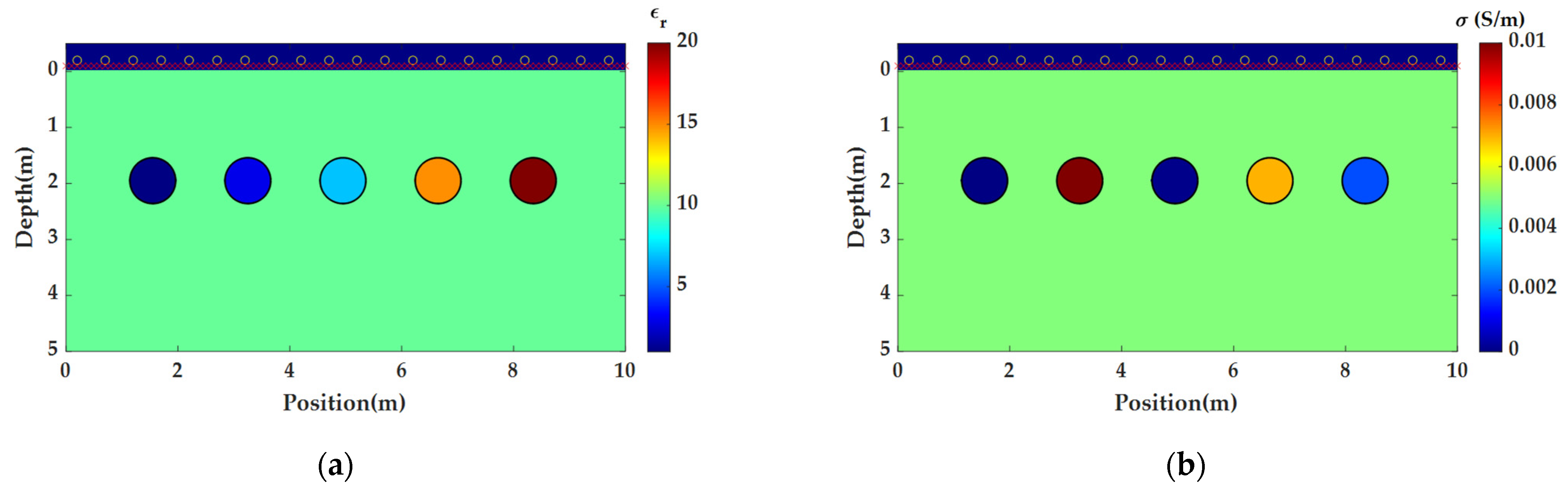
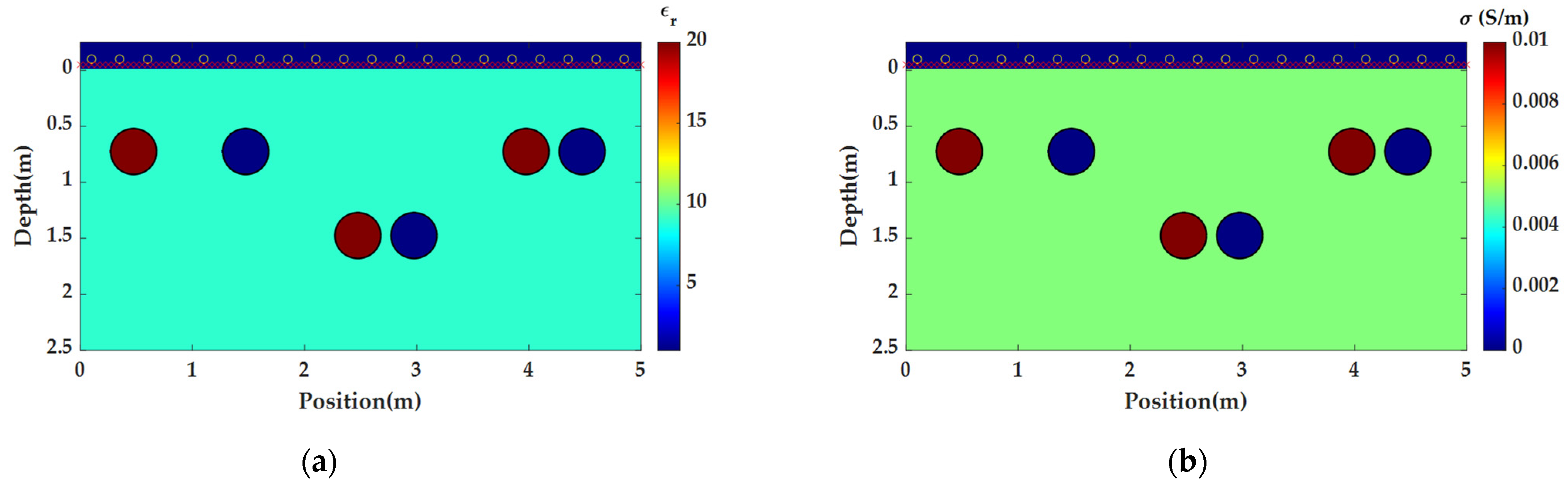
Figure 1 shows the true subsurface models used in the first numerical example. The calculated areas of the models are 10 m long and 5 m deep, and the mesh intervals of the models are 0.05 m in both horizontal and depth axes. The relative permittivity and conductivity of the background medium are 10 and 0.005 S/m. Five circular anomalies, which are considered as parallel pipelines distributed in the direction perpendicular to the transmitter–receiver profile, are placed in the models. The diameters and depths (upper surface) of them are 0.8 m and 1.6 m. The relative permittivity and conductivity of them, from left to right, are 1 and 0 S/m, 3 and 0.01 S/m, 7 and 0.0001 S/m, 15 and 0.007 S/m, and 20 and 0.002 S/m, respectively. There are 20 sources (as shown in yellow $\circ$ in Figure 1) and 100 receivers (as shown in red × in Figure 1) located in the air layer (0.5 m) above the calculation area. The source function is a Ricker wavelet with the dominant frequency equal to 100 MHz, and the observation mode is multi-offset measurement.

As the initial models, we use the homogeneous models with the relative permittivity of 8 (smaller than the background medium) and conductivity of 0.006 S/m (larger than the background medium), which are different from the true models. In the inversion, twelve frequency components (20, 30, 40, 50, 60, 70, 80, 90, 100, 120, 150, and 200 MHz) are used, and the six following frequency strategies are performed: strategy B1, strategy B2, strategy B3, strategy B4, strategy B5, and strategy S, which contain 12, 6, 4, 3, 2, and 1 sub-sequences, respectively, and add 1, 2, 3, 4, 6, and 12 more frequency components at each frequency sub-sequence, respectively. Here, the strategies B refer to the proposed multi-scale cumulative frequency strategy, and the strategy S refers to the simultaneous multi-frequency weighting strategy. The selection method of the inversion sub-sequences of these strategies can be find in Section 2.2.3. The misfit of Φ⁰/Φ^k ≤ 0.00001 is used as the iteration stopping criterion for every sub-sequence in the inversion process. The maximum iteration numbers of each sub-sequence before and in the last frequency sequence are, respectively, set to 100 and 1000.

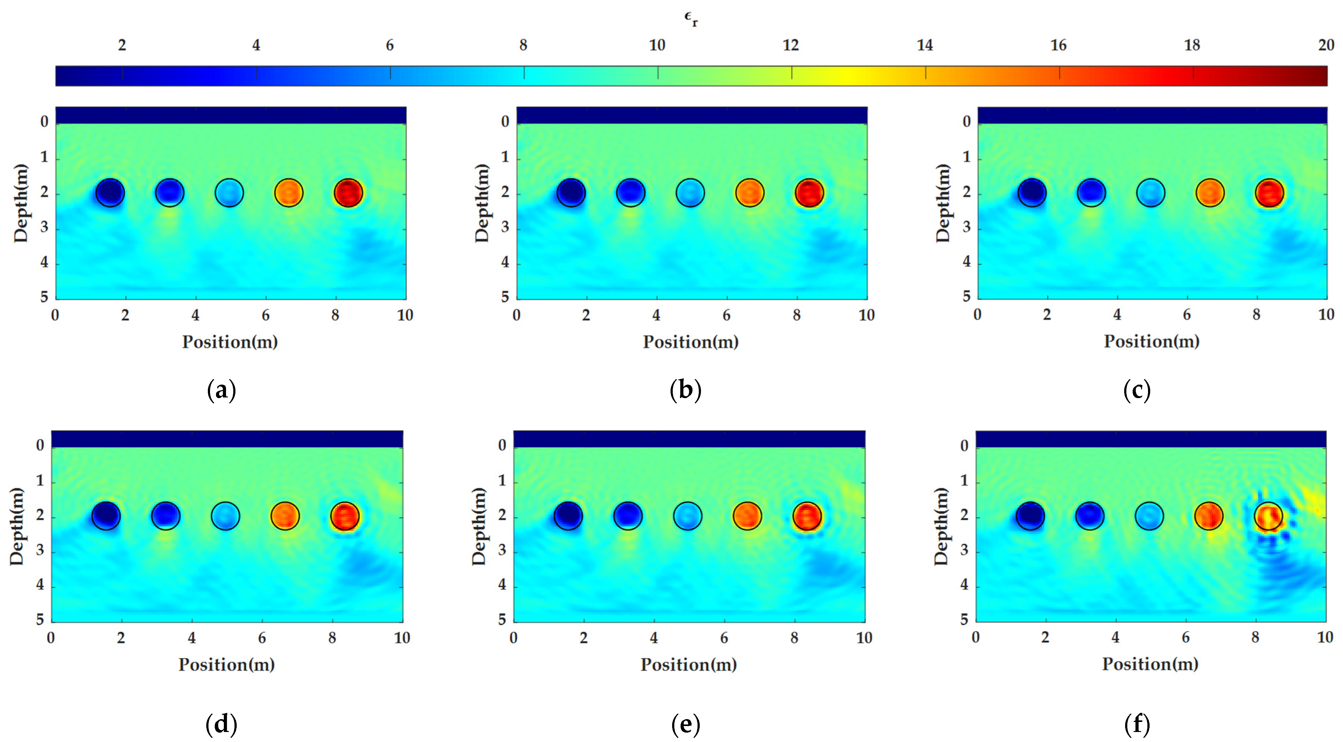
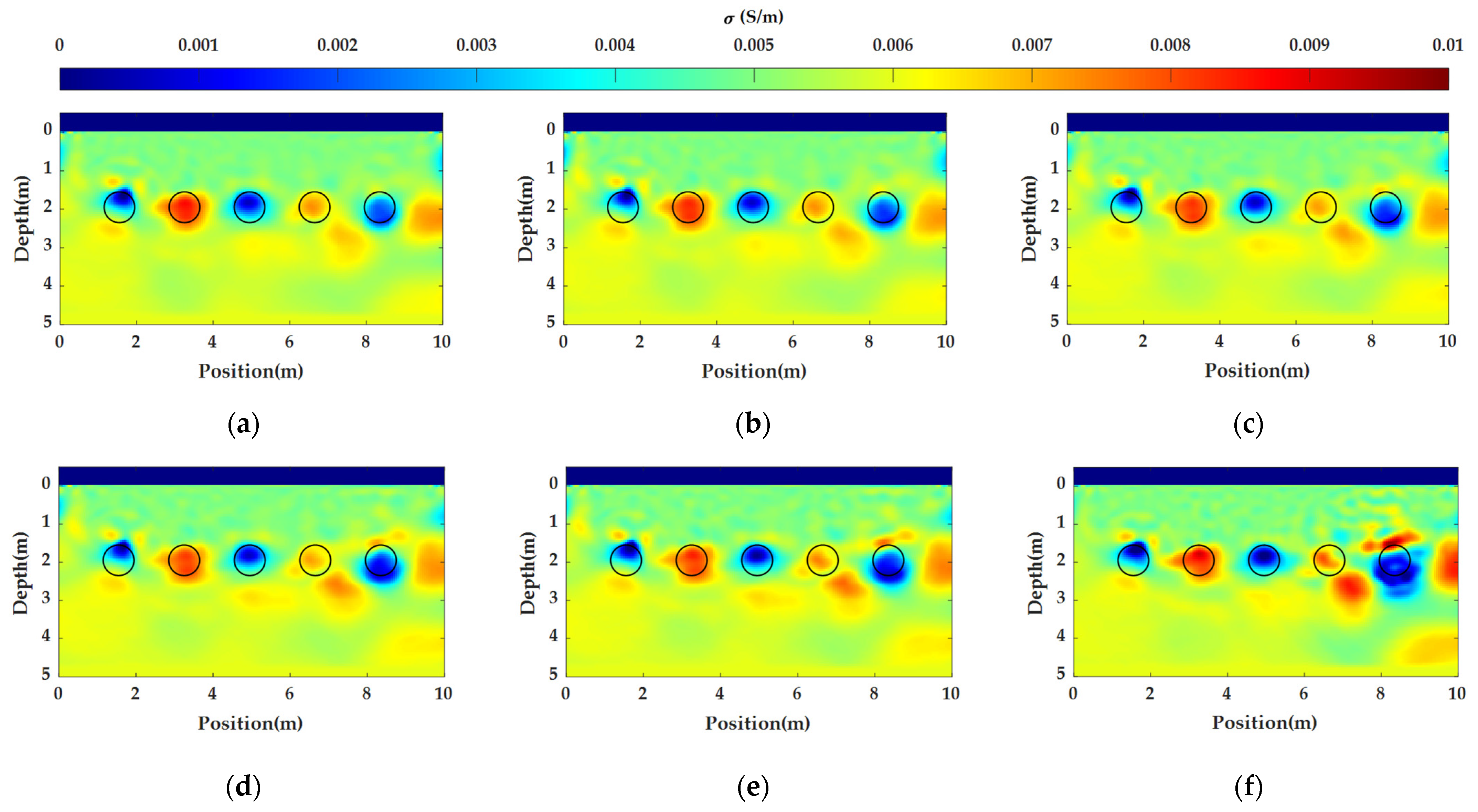
Figure 2 and Figure 3 show the inversion results of the relative permittivity and conductivity of WRI using six different frequency strategies with inaccurate initial models. Overall, the inversion results of the relative permittivity are better than those of the conductivity. In the reconstructed models, the shallow media are reasonable; however, the model media bellow 3 m are far from the true models, among which we notice some artifacts, and the media distribution near the abnormal bodies of conductivity is particularly chaotic. 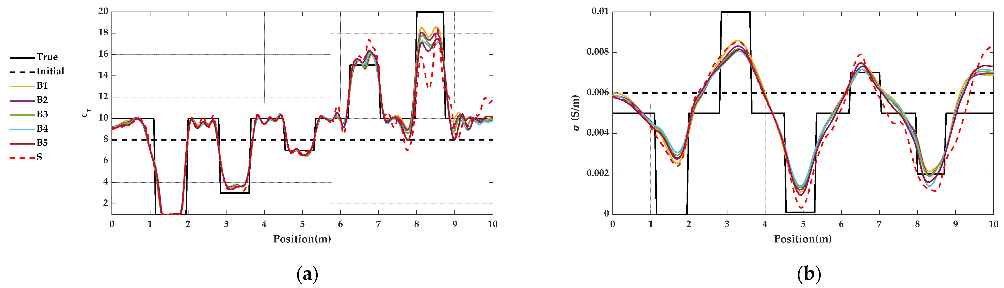Moreover, as the number (N_c in the Section 2.2.3) of the sub-sequences in the inversion decreases, that is, the number (j in the Section 2.2.3) of the added frequency components in each inversion sequence increases, the inversion results are farther away from the true models. Most of the comparison details can be found in the horizontal profiles at a depth of 2 m in Figure 4. The profiles of strategies B1, B2, B3, B4, and B5 maintain a relatively close parameter change trend, and the fewer frequency components accumulated in each frequency cycle, the closer it is to the true model. The profiles of strategy S deviate further from the true model compared with the five strategies mentioned before.

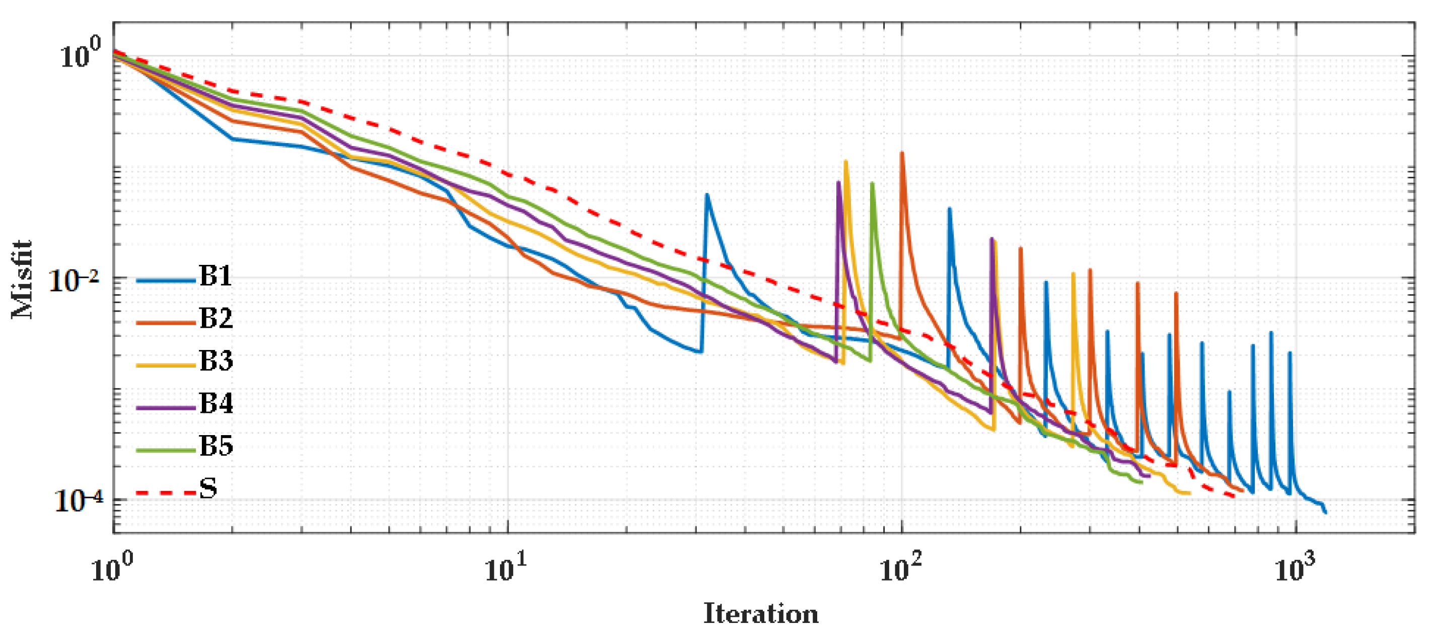
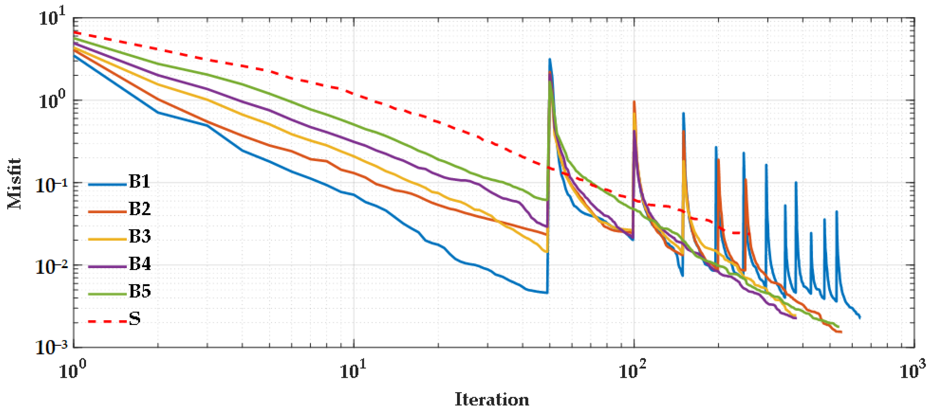
In Figure 5, the misfits under different inversion strategies during the processes are plotted. Obviously, the fewer the frequency components added successively in each frequency sub-sequence, the faster the decline of the misfits in every frequency iteration, but they need more frequency sub-sequences as the iteration proceeds.

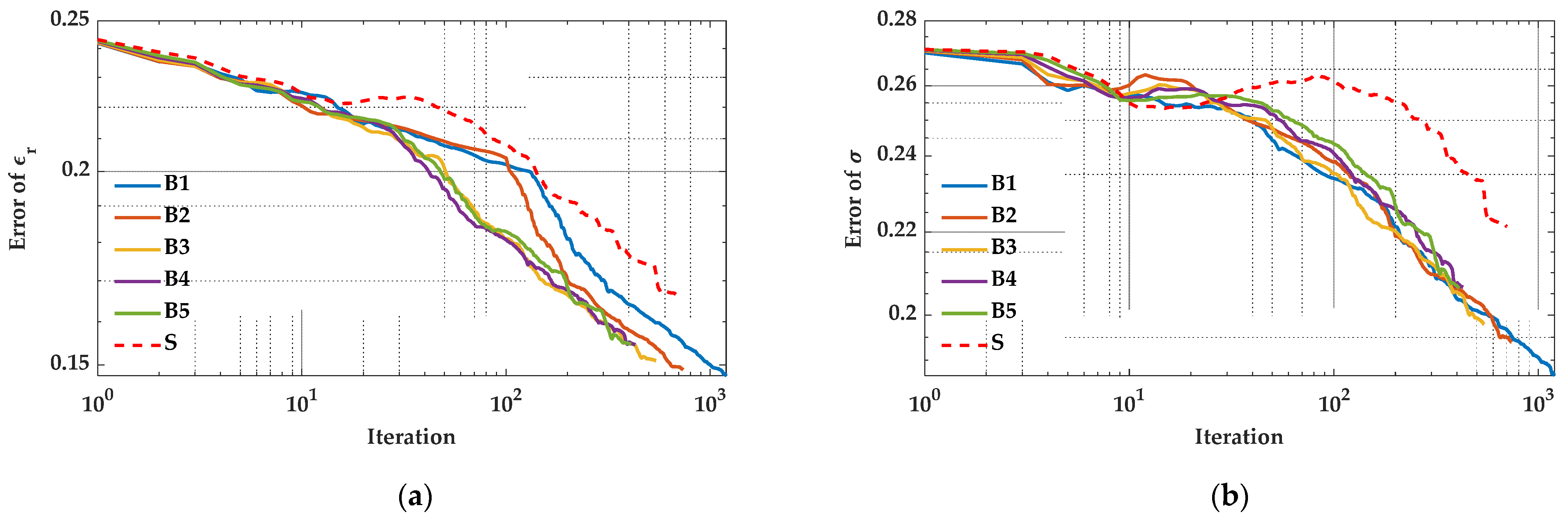
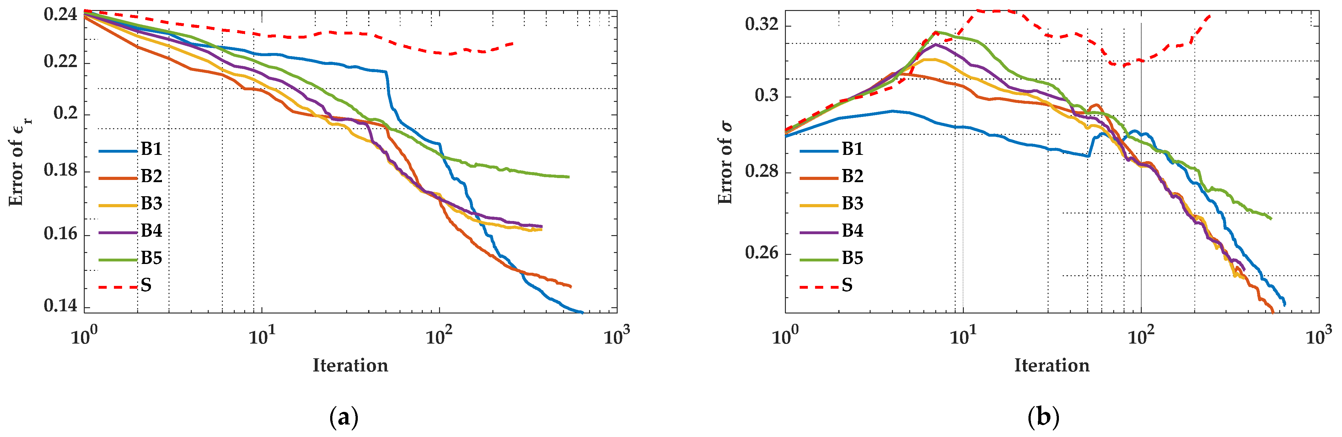
Figure 6 shows the comparison of model reconstruction error curves under different frequency strategies in the inversion process. In the error convergence curves of the reconstructed relative permittivity in Figure 6a, the strategy B1 appears with the smallest final error and largest number of iterations at the end of the optimization; the error convergence trends of B1 and B2 are similar, and the model reconstruction errors are larger than those of other cumulative strategies (B3, B4, B5) under the same number of iterations before the end of inversion; the error convergence trends of B3, B4, and B5 are almost coincident, while the end number of iteration of B3 > B4 > B5, and the end convergence error of B3 < B4 < B5; the reconstruction errors of strategy S in the whole inversion process are larger than those of other frequency strategies. In the error convergence curves of the reconstructed conductivity in Figure 6b, the strategy B1 also appears with the smallest final error and more iterations in the later stage of the optimization due to more frequency sequences; with the increasing of the cumulative frequency components in each sequence, the end errors of B2, B3, B4, and B5 increase slightly, and the end number of the iterations decreases; the reconstruction errors of strategy S increase after 10 iterations and decrease after 100 iteration, but end to a larger convergence error.

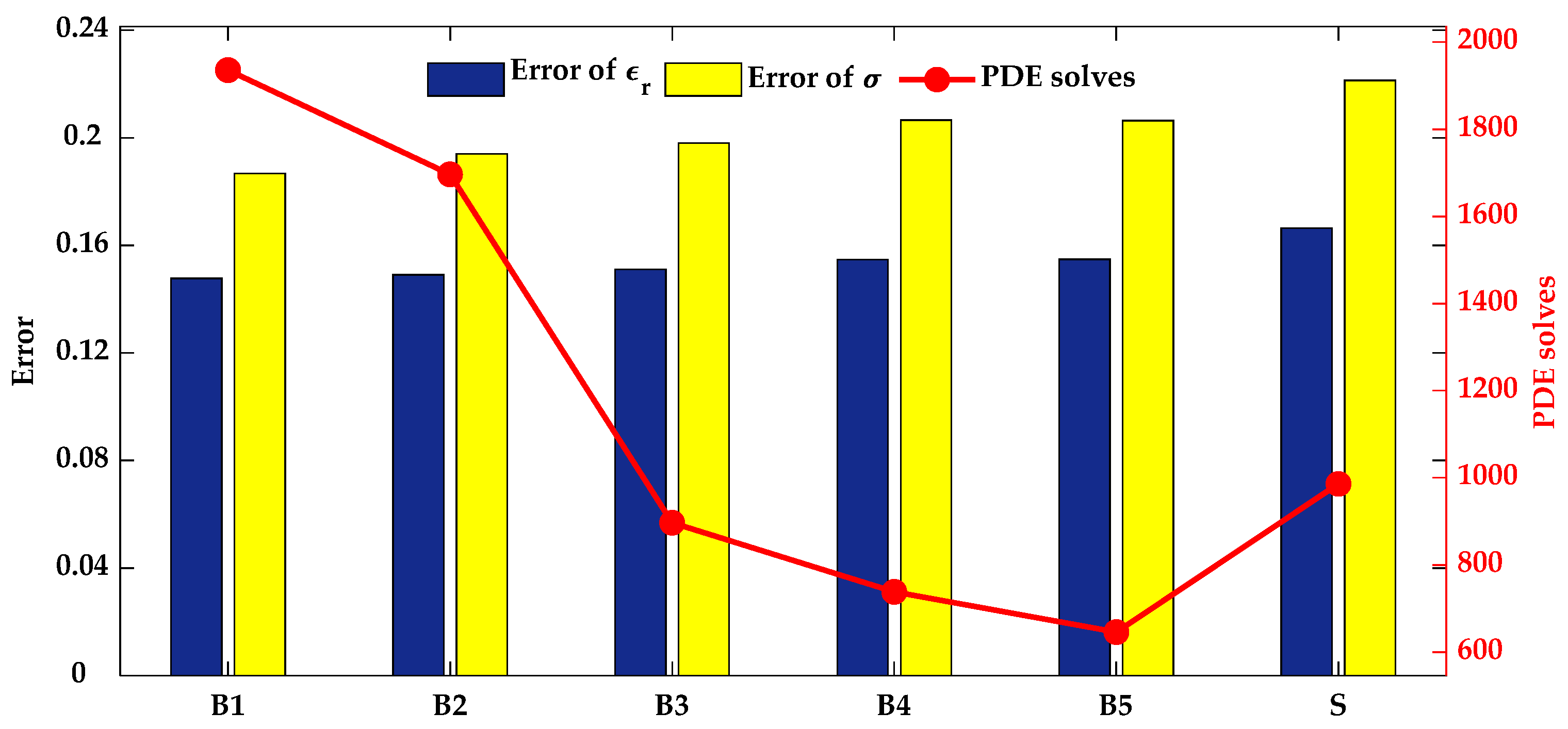
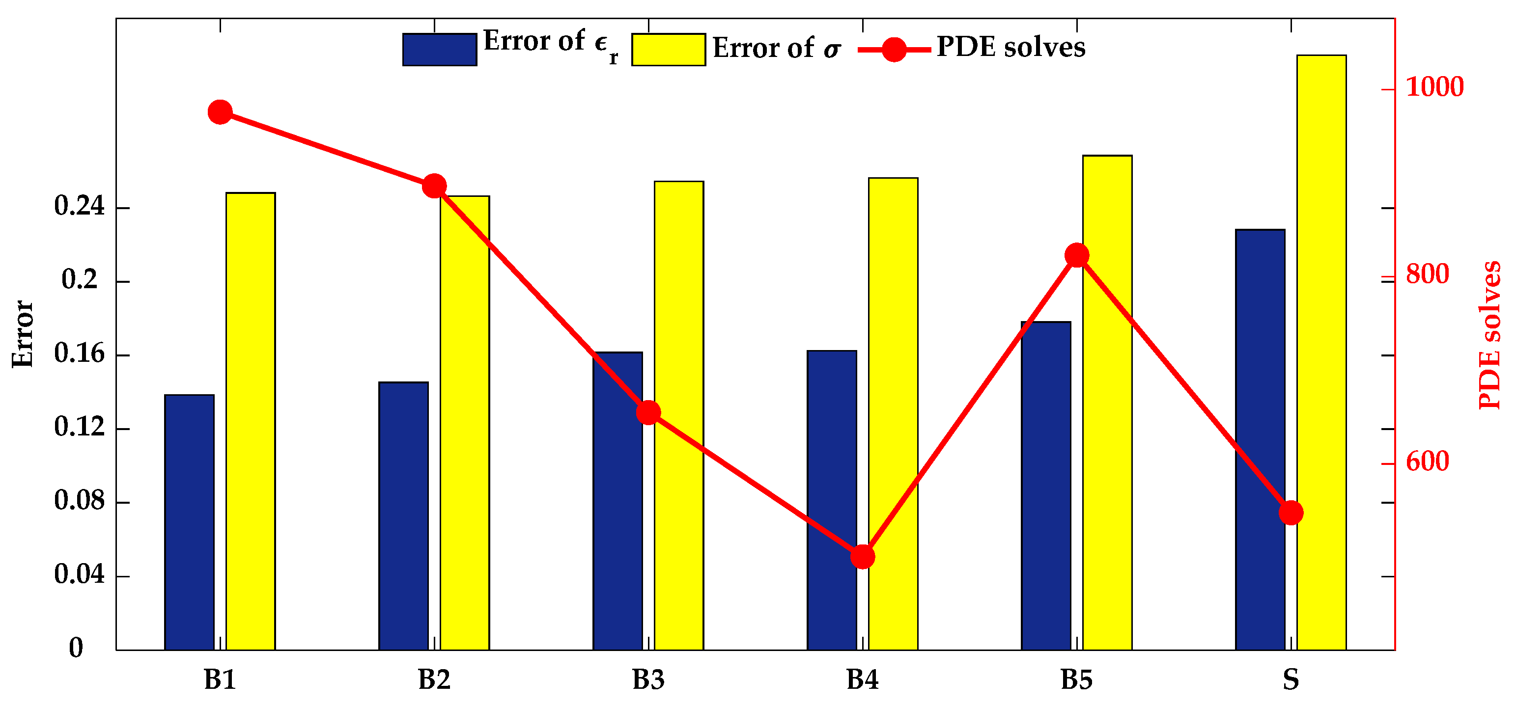
From the bar and marked line display of the model reconstruction error and the number of the PDE calculation at the end iteration of the inversion in Figure 7, in general, the more frequency components added successively in the inversion sub-sequence of the strategies, the larger the model reconstruction errors and the less the PDE solves. Strategies B1, B2, and B3 show better performance in model reconstruction error, and strategies B3, B4, B5, and S need less PDE solves; note that the model reconstruction error of strategy S is large. Therefore, when the initial model is not accurate, we can choose the cumulative frequency strategy and appropriately increase the frequency components in each inversion sub-sequence to reduce the number of iterative solutions, thereby improving the inversion speed.

3.2. Pipelines Model with Different Spacings and Buried Depths

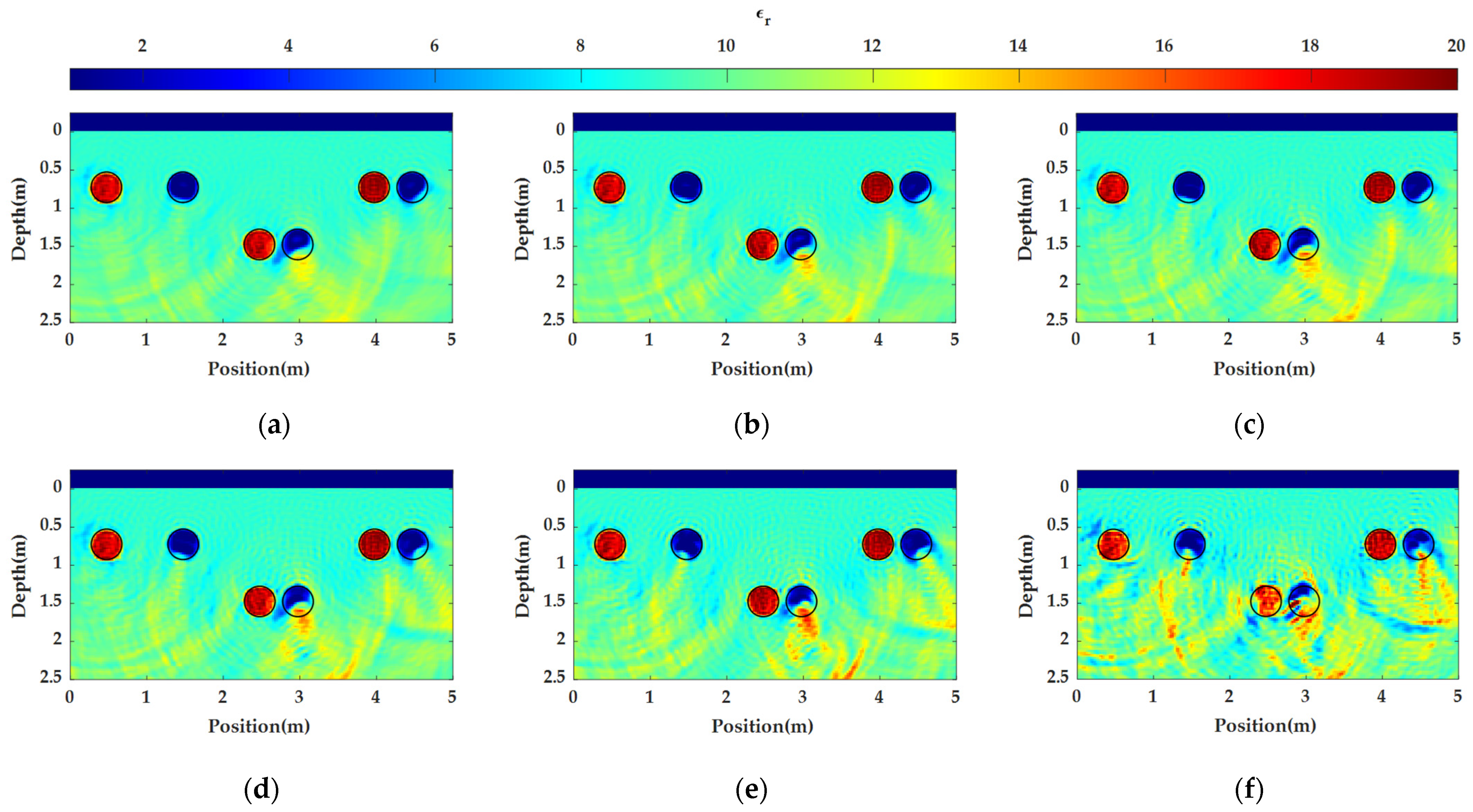
Figure 8 shows the true subsurface models used in the second numerical example. The calculated areas of the models are 5 m long and 2.5 m deep, and the mesh intervals of the models are 0.025 m in both horizontal and depth axes. The relative permittivity and conductivity of the background medium are 9 and 0.005 S/m. Three groups of circular anomalies with different spacing and buried depth, which are considered as pipelines distributed in the direction perpendicular to the transmitter–receiver profile, are placed in the models. The diameters of them are 0.4 m. The spacings of these three groups, from left to right, are 0.6 m, 0.1 m, and 0.1 m, respectively. The depths (upper surface) of these three groups, from left to right, are 0.5 m, 1.3 m, and 0.5 m, respectively. The relative permittivity and conductivity of each group, from left to right, are 20 and 0.01 S/m and 1 and 0 S/m, respectively. As per the first inversion example for the measurements, there are 20 sources (as shown in yellow $\circ$ in Figure 8) and 100 receivers (as shown in red × in Figure 8) located in the air layer (0.25 m) above the calculation area. The source function is a Ricker wavelet with the dominant frequency equal to 400 MHz, and the observation mode is multi-offset measurement.

As the initial models, we use the homogeneous models with the relative permittivity of 10 (larger than the background medium) and conductivity of 0.004 S/m (smaller than the background medium), which are different from the true models. In the inversion, twelve frequency components (40, 80, 120, 160, 200, 240, 280, 320, 360, 400, 500, and 600 MHz) are used, and the six following frequency strategies (as the first example) are performed: strategy B1, strategy B2, strategy B3, strategy B4, strategy B5, and strategy S, which add 1, 2, 3, 4, 6, and 12 more frequency components at each frequency sub-sequence, respectively. The misfit of Φ⁰/Φ^k ≤ 0.00001 is used as the iteration stopping criterion for every sub-sequence in the inversion process. The maximum iteration numbers of each sub-sequence before and in the last frequency sequence are, respectively, set to 50 and 1000.

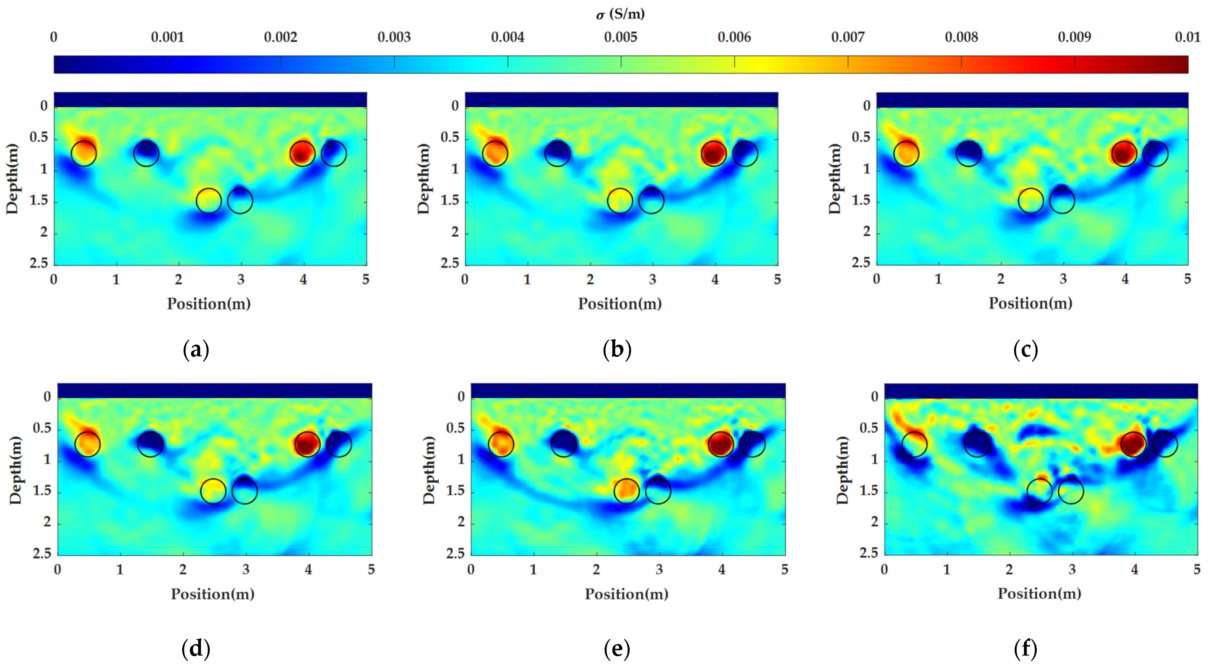
As expected, the inversion results in this case will be similar to those in the first numerical experiment. Figure 9 and Figure 10 show the inversion results of the relative permittivity and conductivity of WRI using six different frequency strategies with inaccurate initial models. 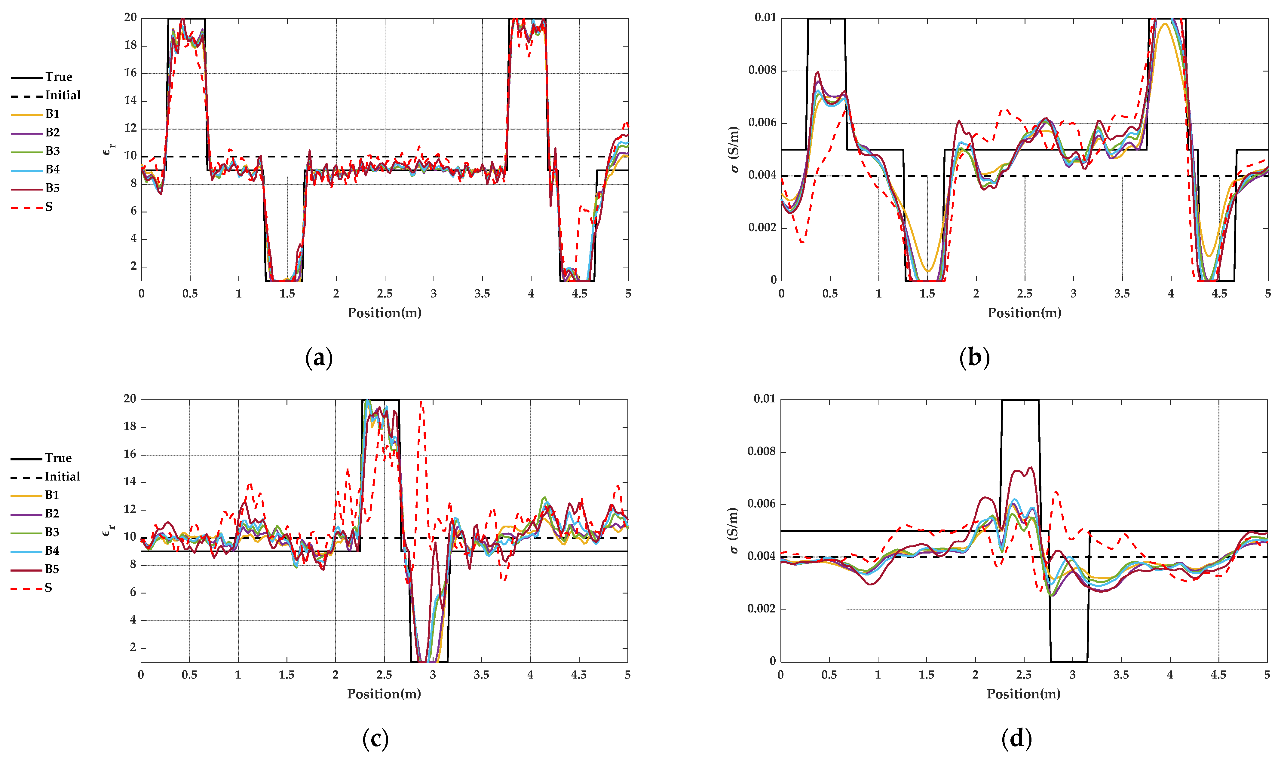These several frequency strategies reconstructed the relative permittivity distribution of the abnormal bodies with different spacings or depths, as shown in Figure 9, but the recovery of the pipe objects near the boundary of the model is poor due to the limited observation angle. Although the model media of the background below 1.5 m are far from the true models, the reconstructed abnormal bodies are close to the true models. However, the reconstruction results of the anomalous bodies of conductivity model are worse than those of relative permittivity, especially for deep anomalous bodies. More comparison details can also be found in the horizontal profiles at a depth of 0.75 m and 1.5 m in Figure 11. With the increase of the frequency components accumulated in each frequency cycle, there are more disturbances in the profiles of the reconstructed models, especially the strategy S.

In Figure 12, the misfits under different inversion strategies during the process are plotted, of which the trends are similar to that in the first numerical example shown in Figure 5. Figure 13 shows the comparison of model reconstruction error curves under different frequency strategies in the inversion process. In the error convergence curves of the reconstructed relative permittivity in Figure 13a, strategy B1 showed the smallest final error and largest number of iterations at the end of the optimization. The error convergence trends of B2, B3, and B4 are almost coincident (expect B5), while the end number of iteration of B2 > B5 > B3 > B4, and the end convergence error of B2 < B3 < B4 < B5. The reconstructed errors of strategy S in the whole inversion process are larger than those of other frequency strategies. In the error convergence curves of the reconstructed conductivity in Figure 13b, strategies B1 and B2 show the smaller final error and more iterations in the later stage of the optimization due to more frequency sequences. With the increasing of the cumulative frequency components in each sequence, the end errors of B3, B4, and B5 increase slightly, and the end numbers of the iterations decrease. The reconstructed error of strategy S begins to decline after 10 iterations but changes to an increasing trend after 70 iterations, and it remains as the maximum one almost throughout the whole process.

From the bar and marked line display of the model reconstruction error and the number of the PDE calculation at the end iteration of the inversion in Figure 14, in general, the more frequency components added successively in the inversion sub-sequence of the strategies, the larger the model reconstruction errors and the less the PDE solves. Strategies B1 and B2 show better performance in model reconstruction error, and strategies B3, B4, and S need less PDE solves; note that the model reconstruction errors of strategy S are large.

3.3. Physical Pipelines Model with Field Data

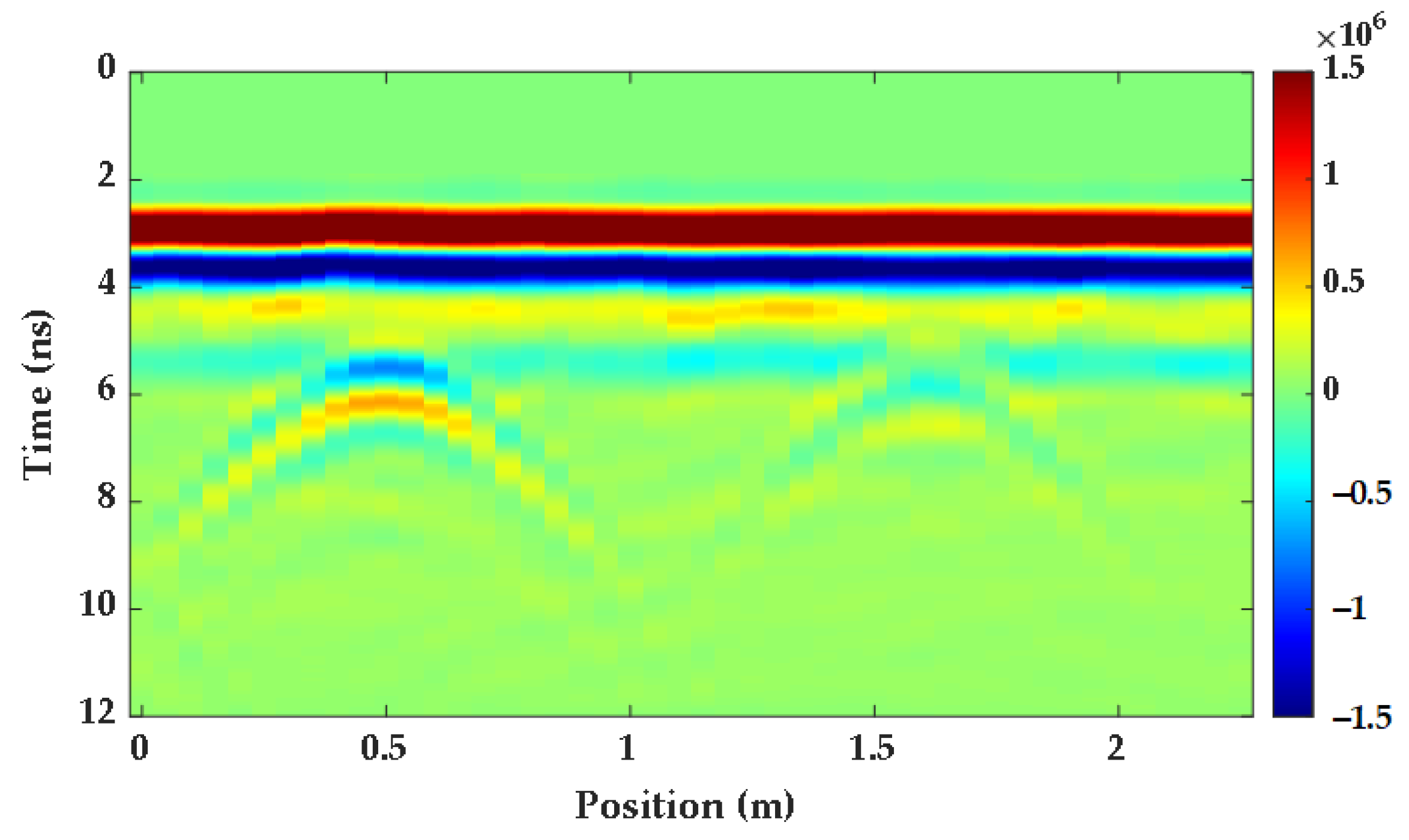
For further advancing the high-precision interpretation of GPR data of subsurface pipelines, a preliminary test was performed in the field GPR data, as shown in Figure 15. The measured data were collected in the physical model laboratory. Specifically, in the sand tank filled with uniform dry quartz sand, we buried two plastic pipes. The left one is an empty pipe with a diameter of 0.12 m, and the right one is a plastic pipe with a diameter of 0.08 m filled with soil. Their buried depths were 0.13 m. Geophysical survey Systems Inc. (GSSI), Nashua, NH, USA, 900 MHz antenna is used for data acquisition. The trace interval is set to 0.05 m, the time window is set to 12 ns, and a total of 46 traces of data are collected.

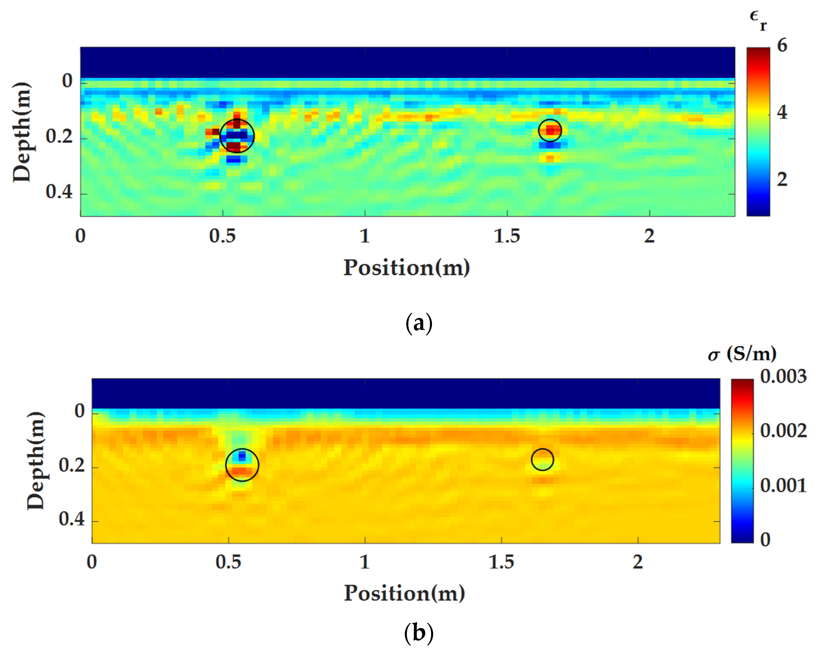
In the inversion process, the calculated areas of the models are 2.3 m long and 0.48 m deep, and the mesh intervals of the models are 0.025 m in both horizontal and depth axes. There are 46 sources and receivers located in the air layer (0.125 m) above the calculation area. The initial model is a uniform medium, and its relative permittivity and conductivity of the background medium are set to 3.4 (calculated by the hyperbolic fitting method) and 0.005 S/m (set according to our previous experiments), respectively. The observation data were converted to the frequency domain by fast Fourier transform before inversion; in the inversion, we use fifteen frequency components (88.6, 177.2, 265.7, 354.3, 442.9, 531.5, 620.1, 708.7, 797.2, 885.8, 974.4, 1063.0, 1151.6, 1240.1, and 1328.7 MHz), and the inversion takes 60 iterations and 23.46 min.

Figure 16 shows the inversion results of the relative permittivity and conductivity, where the black hollow circles in the reconstructed models indicate the correct locations of the pipes. Obviously, from the B-Scan profile of data in Figure 15, it is difficult to identify the material, buried depth, or the diameter of the pipes directly and accurately. However, in Figure 16, we can roughly determine these parameters, although there are some false anomalies or artifacts. 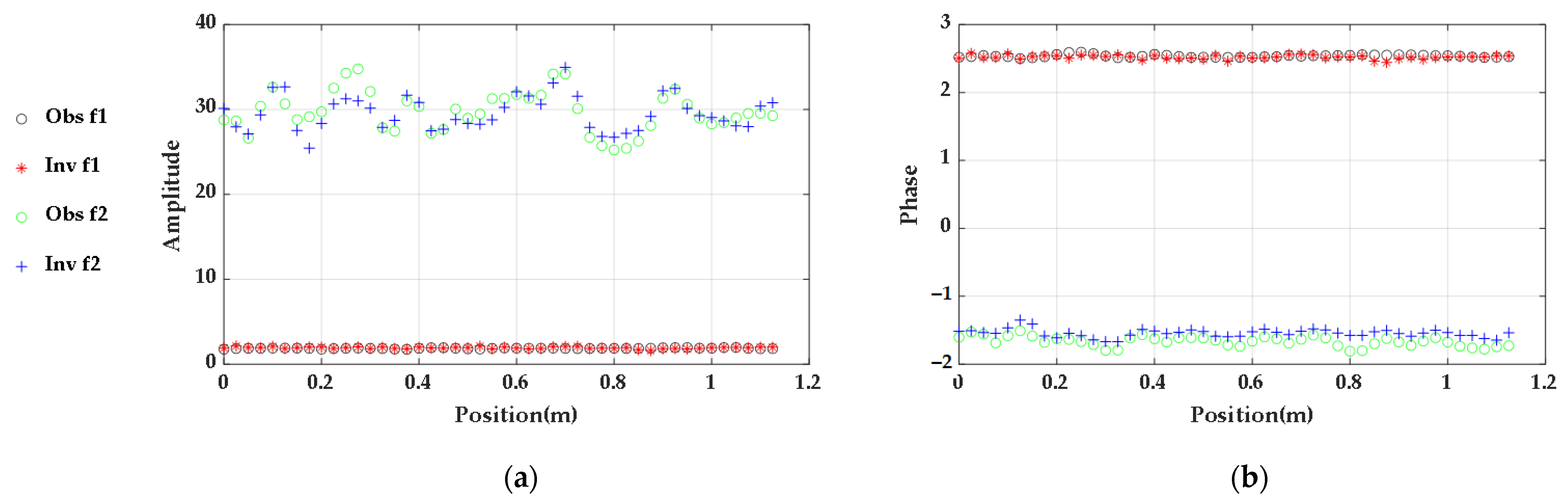Figure 17 shows the spectrums and phases of the frequency observation data and the calculation data of the final inversion results at two different frequencies (265.7 MHz and 708.7 MHz). In different positions, the spectrums and phases of lower frequency field data basically coincide with the simulated data, while there are certain differences of higher frequency data. The above results show that the proposed algorithm has good applicability to the field data.

4. Discussion

To sum up the experiences of the numerical experiments in the paper, by accumulating the higher frequency components step by step in the proposed multi-scale cumulative frequency strategy, each inversion sub-sequence is equivalent to provide a better initial model for the next sub-sequence. Thus, the performed inversion is more accurate and stable than the simultaneous multi-frequency strategy. Specifically, the fact is that to increase the number of additional frequency components in each frequency sub-sequence will shorten the number of iterations, but it results in an increase of reconstruction errors. At this point, man can obviously assume that a compromise between the precision of results and the number of iterations should be found to enhance the inversion method. The suggestion from this study is that, in most situations, we can choose a cumulative frequency strategy and appropriately increase the frequency components in each inversion sub-sequence.

It should be noted that the case studies presented in this paper used the initial models different from the background media of the true models. In example 1, the relative permittivity of the initial model < the true model, and the conductivity of the initial model > the true model. In example 2, the relative permittivity of the initial model > the true model, and the conductivity of the initial model < the true model. When comparing the inversion effects of different frequency strategies, the frequency components used in example 1 had more low-frequency components, and the maximum iteration number of each sub-sequence before the last frequency sequence in example 1 and example 2 were set to 100 and 50, respectively. This means that the nonlinearity of the second numerical experiment was more serious. In example 1, the model-reconstructed errors of our proposed strategy (B1, B2, B3, B4, and B5) were reduced by about 7~11% (relative permittivity) or 7~15% (conductivity) more than strategy S. In example 2, the model-reconstructed errors of our proposed strategy (B1, B2, B3, B4, and B5) were reduced by about 20~40% (relative permittivity) or 17~24% (conductivity) more than strategy S. From the inversion results, we found that the conclusions of these two numerical experiments were similar, which proved that our proposed strategy and conclusion could be popularized.

In addition, the inversion of the field data also verified the feasibility of our proposed strategy. However, there are still some pressing problems that need to be solved in the WRI strategy proposed in this paper for GPR data. For example, there are numerical oscillations and artifacts in the inversion model. For solving this problem, we have made a preliminary exploration in another work [14] that is an appropriate regularization able to eliminate some inaccurate inversion trends [14,32]. Secondly, in view of the reconstruction effect of deep media in the inversion, the depth-weighting scheme can be considered to improve it. Thirdly, the parameters of real underground media often change with frequency, while our assumption of the parameters (e.g., the relative permittivity is a constant) is not correct. This will lead to a stronger contribution of high-frequency components than reality. Furthermore, in order to expand the scope of this study to adapt to the situation where the wavelet of field data is always difficult to estimate [39], it is important to develop an efficient wavelet-independent WRI scheme to improve the accuracy of the inversion of the measured data. Finally, it is necessary to research an efficient optimization algorithm suitable for the WRI system, which is vital for the calculation of the inversion process.

5. Conclusions

In this paper, we proposed a WRI scheme in the frequency domain for the permittivity and conductivity reconstruction of urban underground pipeline GPR data based on a multi-scale cumulative frequency strategy. The solution of the WRI optimization problem was performed by the variable projection method, and the frequency inversion method combined the cumulative sequential strategy and simultaneous multi-frequency weighting strategy.

The inversion results of the first two numerical examples with different types of pipelines showed that our proposed algorithm can effectively reconstruct the medium distribution and physical parameters of underground pipelines, and the combination of WRI and the multi-scale cumulative frequency strategy can greatly improve the accuracy and stability of the inversion. Moreover, the inversion results of the field data further verified the feasibility and confirmed the potential application prospect of this method in future work.

This study, as well as the discussion on the inversion strategies, could motivate research into its reliable application within the domain of engineering practice (not only of the pipeline detection but also of the urban underground space exploration). What should be mentioned is that this paper only analyzed the frequency strategy in the inversion in detail, which is only a small part of the high-precision inversion research. Further exploration would be focused on the regularization strategies, the wavelet estimation, the depth-weighting methods, the optimization algorithms, etc.