
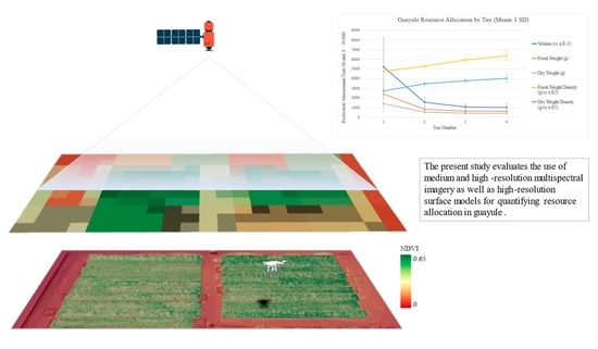
Estimating Productivity Measures in Guayule Using UAS Imagery and Sentinel-2 Satellite Data

 ,
,
Abstract
:
1. Introduction
2. Materials and Methods
2.1. Field Site
2.2. Equipment
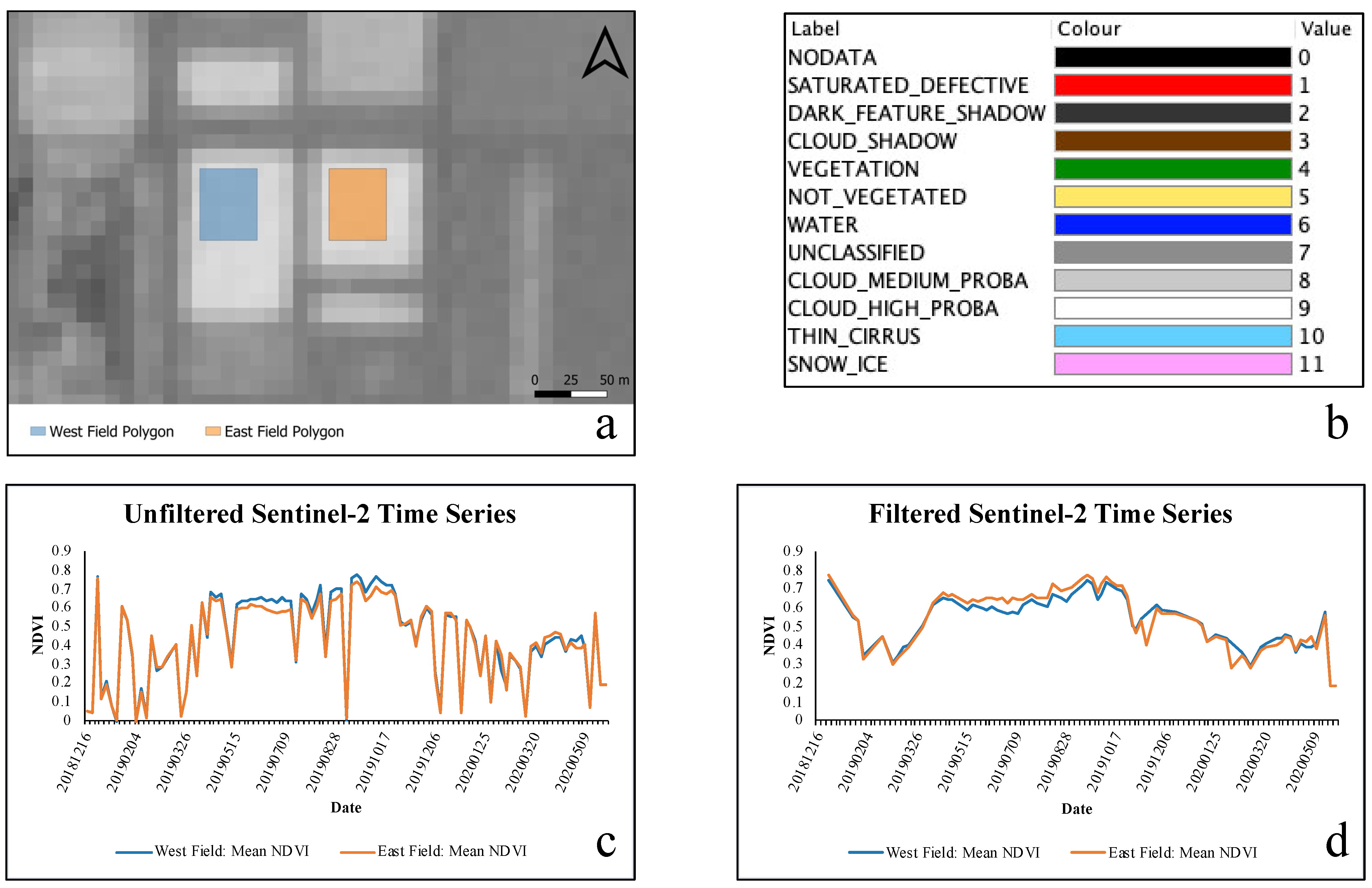
2.3. Georeferencing
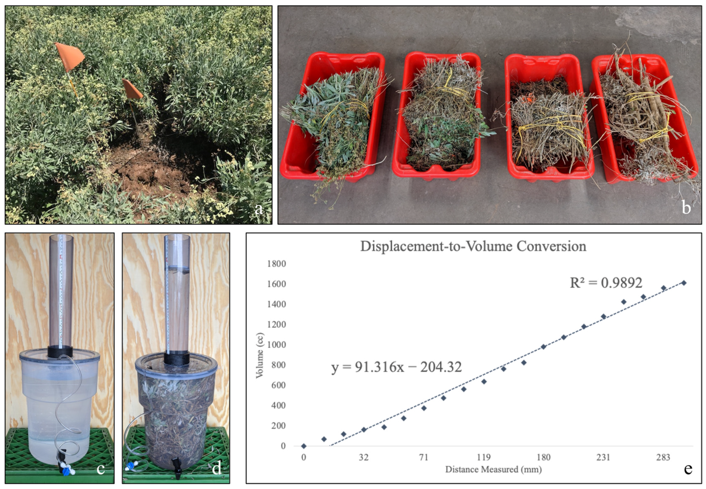
2.4. Harvest and Fresh Weight Measurements
2.5. Volumetric Measurements
2.6. Dry Weight Measurements
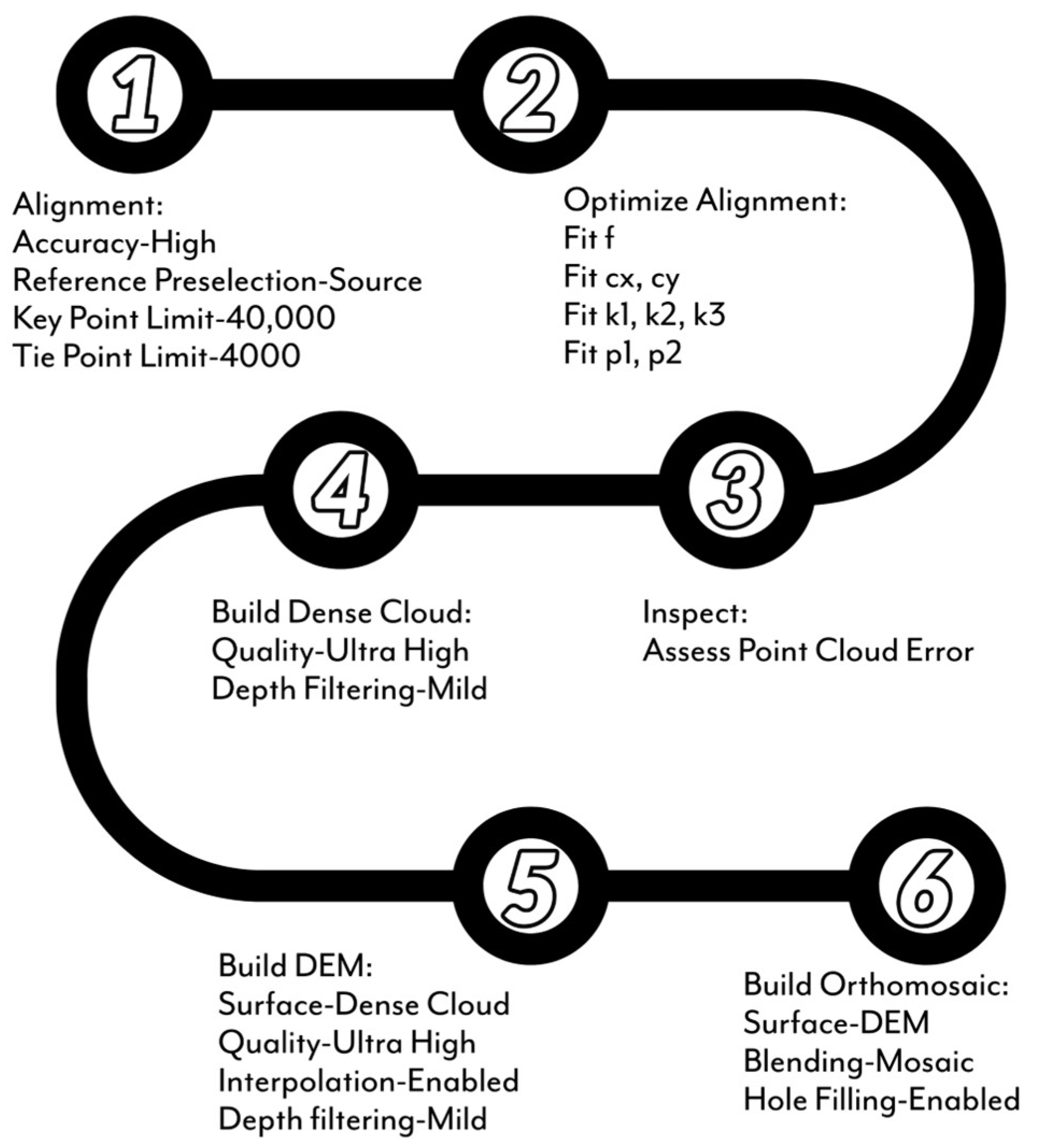
2.7. RGB Image Processing
2.8. Multispectral Image Processing
2.9. Canopy Height Model
2.10. Statistical Analyses
3. Results
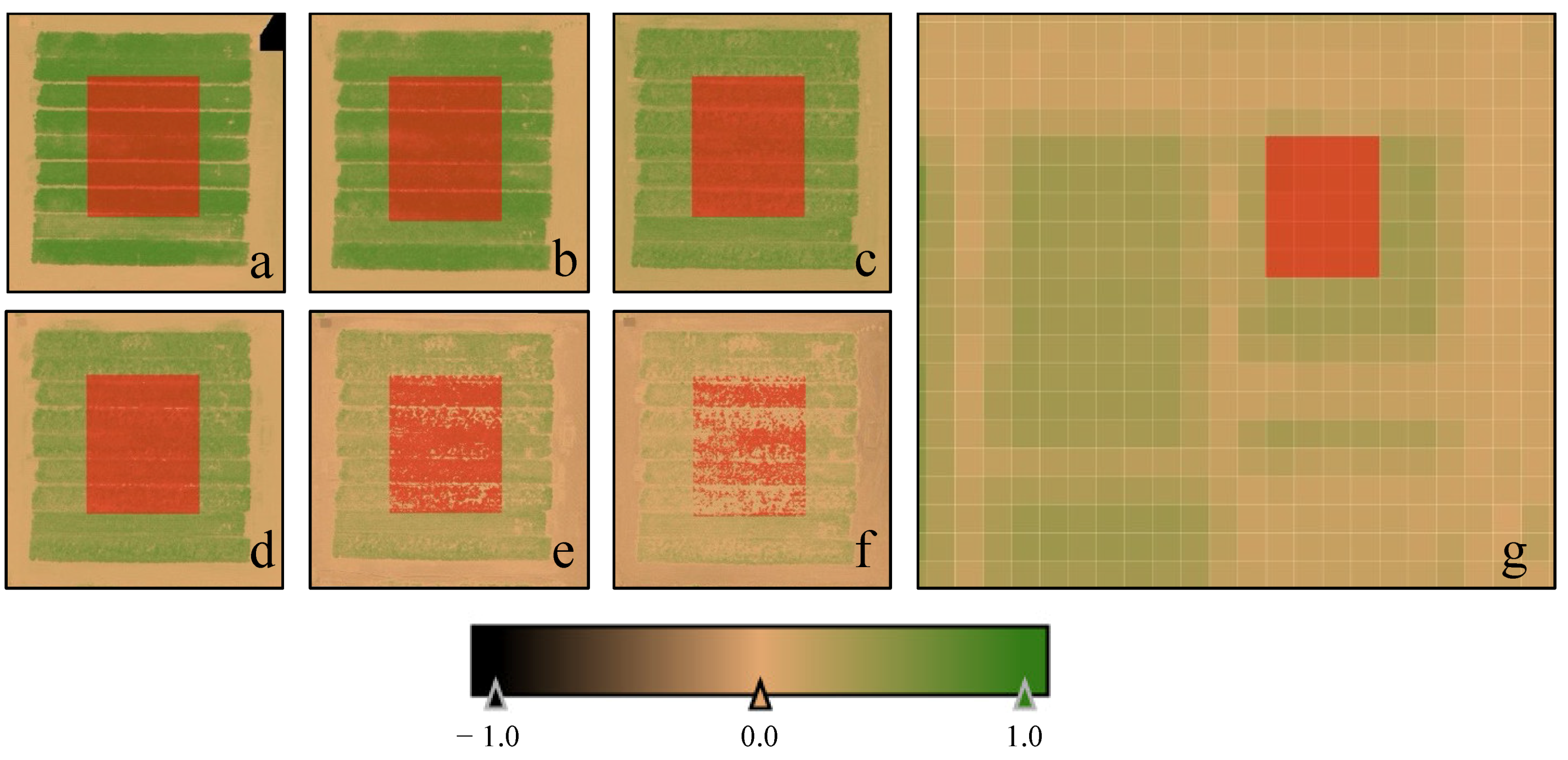
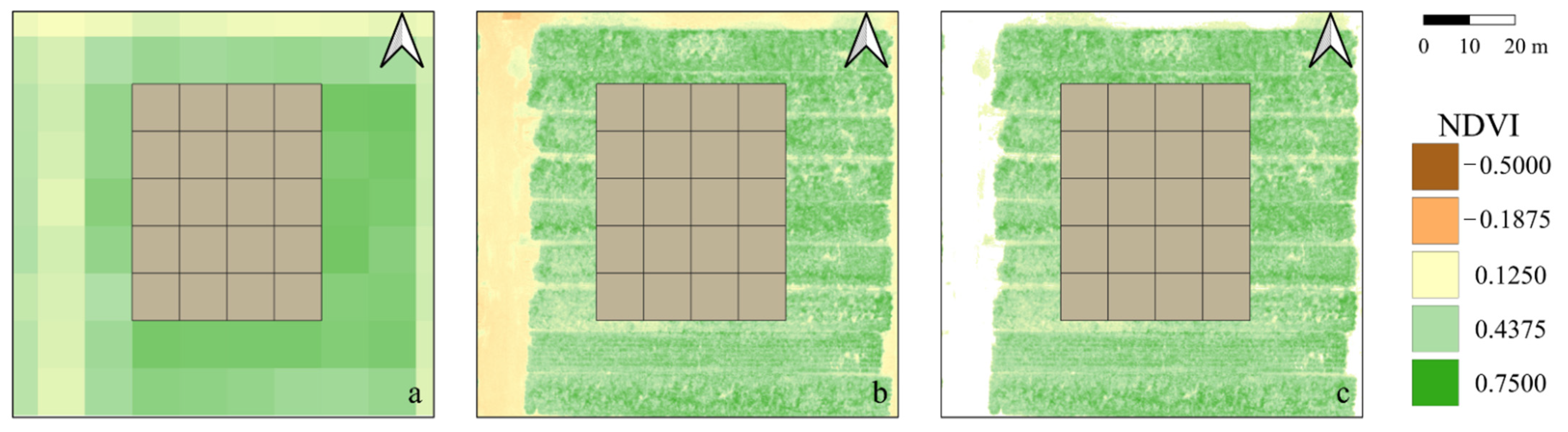
3.1. Geospatial Error
3.2. Crop Productivity Measurements
3.3. UAS Model Selection and Performance
3.4. Scaled Model Performance
4. Discussion
5. Conclusions
6. Patents
Author Contributions
Funding
Data Availability Statement
Acknowledgments
Conflicts of Interest
References
- Daponte, P.; De Vito, L.; Glielmo, L.; Iannelli, L.; Liuzza, D.; Picariello, F.; Silano, G. A Review on the Use of Drones for Precision Agriculture. IOP Conf. Ser. Earth Environ. Sci. 2019, 275, 012022. [Google Scholar] [CrossRef]
- Spalević, Ž.; Ilić, M.; Savija, V. The Use of Drones in Agriculture: ICT Policy, Legal and Economical Aspects. Ekonomika 2018, 64, 93–107. [Google Scholar] [CrossRef] [Green Version]
- Rasutis, D.; Soratana, K.; McMahan, C.; Landis, A.E. A Sustainability Review of Domestic Rubber from the Guayule Plant. Ind. Crops Prod. 2015, 70, 383–394. [Google Scholar] [CrossRef]
- Ilut, D.C.; Sanchez, P.L.; Coffelt, T.A.; Dyer, J.M.; Jenks, M.A.; Gore, M.A. A Century of Guayule: Comprehensive Genetic Characterization of the US National Guayule (Parthenium Argentatum A. Gray) Germplasm Collection. Ind. Crops Prod. 2017, 109, 300–309. [Google Scholar] [CrossRef]
- van Beilen, J.B.; Poirier, Y. Guayule and Russian Dandelion as Alternative Sources of Natural Rubber. Crit. Rev. Biotechnol. 2007, 27, 217–231. [Google Scholar] [CrossRef]
- Foster, M.A.; Coffelt, T.A. Guayule Agronomics: Establishment, Irrigated Production, and Weed Control. Ind. Crops Prod. 2005, 22, 27–40. [Google Scholar] [CrossRef]
- Estilai, A.; Ehdaie, B.; Naqvi, H.H.; Dierig, D.A.; Ray, D.T.; Thomson, A.E. Correlations and Path Analyses of Agronomic Traits in Guayule. Crop Sci. 1992, 32, 953–957. [Google Scholar] [CrossRef]
- Veatch-Blohm, M.E.; Ray, D.T.; McCloskey, W.B. Water-Stress-Induced Changes in Resin and Rubber Concentration and Distribution in Greenhouse-Grown Guayule. Agron. J. 2006, 98, 766–773. [Google Scholar] [CrossRef]
- Dierig, D.A.; Thompson, A.E.; Ray, D.T. Relationship of Morphological Variables to Rubber Production in Guayule. Euphytica 1989, 44, 259–264. [Google Scholar] [CrossRef]
- Kuruvadi, S.; Jasso Cantu, D.; Angulo-Sanchez, J.L. Rubber Content in Different Plant Parts and Tissues of Mexican Guayule Shrubs. Ind. Crops Prod. 1997, 7, 19–25. [Google Scholar] [CrossRef]
- Catchpole, W.R.; Wheeler, C.J. Estimating Plant Biomass: A Review of Techniques. Aust. J. Ecol. 1992, 17, 121–131. [Google Scholar] [CrossRef]
- Zhao, D.; Glaz, B.; Edme, S.; Del Blanco, I. Precision of Sugarcane Biomass Estimates in Pot Studies Using Fresh and Dry Weights. J. Am. Soc. Sugar Cane Technol. 2010, 30, 37. [Google Scholar]
- de Carvalho, E.X.; Menezes, R.S.C.; de Sá Barreto Sampaio, E.V.; Neto, D.E.S.; Tabosa, J.N.; de Oliveira, L.R.; Simões, A.L.; Sales, A.T. Allometric Equations to Estimate Sugarcane Aboveground Biomass. Sugar Tech 2019, 21, 1039–1044. [Google Scholar] [CrossRef]
- Kuyah, S.; Dietz, J.; Muthuri, C.; Jamnadass, R.; Mwangi, P.; Coe, R.; Neufeldt, H. Allometric Equations for Estimating Biomass in Agricultural Landscapes: I. Aboveground Biomass. Agric. Ecosyst. Environ. 2012, 158, 216–224. [Google Scholar] [CrossRef]
- Murray, R.B.; Jacobson, M.Q. An Evaluation of Dimension Analysis for Predicting Shrub Biomass. J. Range Manag. 1982, 35, 451. [Google Scholar] [CrossRef]
- Kumar, L.; Mutanga, O. Remote Sensing of Above-Ground Biomass. Remote Sens. 2017, 9, 935. [Google Scholar] [CrossRef] [Green Version]
- Brocks, S.; Bendig, J.; Bareth, G. Toward an Automated Low-Cost Three-Dimensional Crop Surface Monitoring System Using Oblique Stereo Imagery from Consumer-Grade Smart Cameras. J. Appl. Remote Sens 2016, 10, 046021. [Google Scholar] [CrossRef] [Green Version]
- da Cunha, J.P.A.R.; Sirqueira Neto, M.A.; Hurtado, S.M.C. Estimating Vegetation Volume of Coffee Crops Using Images from Unmanned Aerial Vehicles. Eng. Agríc. 2019, 39, 41–47. [Google Scholar] [CrossRef]
- Ehlert, D.; Horn, H.-J.; Adamek, R. Measuring Crop Biomass Density by Laser Triangulation. Comput. Electron. Agric. 2008, 61, 117–125. [Google Scholar] [CrossRef]
- Iqbal, F.; Lucieer, A.; Barry, K.; Wells, R. Poppy Crop Height and Capsule Volume Estimation from a Single UAS Flight. Remote Sens. 2017, 9, 647. [Google Scholar] [CrossRef] [Green Version]
- Lati, R.N.; Manevich, A.; Filin, S. Three-Dimensional Image-Based Modelling of Linear Features for Plant Biomass Estimation. Int. J. Remote Sens. 2013, 34, 6135–6151. [Google Scholar] [CrossRef]
- Eltner, A.; Sofia, G. Structure from Motion Photogrammetric Technique. In Developments in Earth Surface Processes; Elsevier: Amsterdam, The Netherlands, 2020; Volume 23, pp. 1–24. ISBN 978-0-444-64177-9. [Google Scholar]
- Christiansen, M.; Laursen, M.; Jørgensen, R.; Skovsen, S.; Gislum, R. Designing and Testing a UAV Mapping System for Agricultural Field Surveying. Sensors 2017, 17, 2703. [Google Scholar] [CrossRef] [Green Version]
- Eitel, J.U.H.; Magney, T.S.; Vierling, L.A.; Brown, T.T.; Huggins, D.R. LiDAR Based Biomass and Crop Nitrogen Estimates for Rapid, Non-Destructive Assessment of Wheat Nitrogen Status. Field Crops Res. 2014, 159, 21–32. [Google Scholar] [CrossRef]
- Obanawa, H.; Yoshitoshi, R.; Watanabe, N.; Sakanoue, S. Portable LiDAR-Based Method for Improvement of Grass Height Measurement Accuracy: Comparison with SfM Methods. Sensors 2020, 20, 4809. [Google Scholar] [CrossRef] [PubMed]
- Wallace, L.; Lucieer, A.; Malenovský, Z.; Turner, D.; Vopěnka, P. Assessment of Forest Structure Using Two UAV Techniques: A Comparison of Airborne Laser Scanning and Structure from Motion (SfM) Point Clouds. Forests 2016, 7, 62. [Google Scholar] [CrossRef] [Green Version]
- Carlson, T.N.; Ripley, D.A. On the Relation between NDVI, Fractional Vegetation Cover, and Leaf Area Index. Remote Sens. Environ. 1997, 62, 241–252. [Google Scholar] [CrossRef]
- Jin, H.; Eklundh, L. A Physically Based Vegetation Index for Improved Monitoring of Plant Phenology. Remote Sens. Environ. 2014, 152, 512–525. [Google Scholar] [CrossRef]
- Olson, D.; Chatterjee, A.; Franzen, D.W.; Day, S.S. Relationship of Drone-Based Vegetation Indices with Corn and Sugarbeet Yields. Agron. J. 2019, 111, 2545–2557. [Google Scholar] [CrossRef]
- Stavrakoudis, D.; Katsantonis, D.; Kadoglidou, K.; Kalaitzidis, A.; Gitas, I. Estimating Rice Agronomic Traits Using Drone-Collected Multispectral Imagery. Remote Sens. 2019, 11, 545. [Google Scholar] [CrossRef] [Green Version]
- Schaefer, M.; Lamb, D. A Combination of Plant NDVI and LiDAR Measurements Improve the Estimation of Pasture Biomass in Tall Fescue (Festuca arundinacea Var. Fletcher). Remote Sens. 2016, 8, 109. [Google Scholar] [CrossRef] [Green Version]
- Tilly, N.; Aasen, H.; Bareth, G. Fusion of Plant Height and Vegetation Indices for the Estimation of Barley Biomass. Remote Sens. 2015, 7, 11449–11480. [Google Scholar] [CrossRef] [Green Version]
- Viljanen, N.; Honkavaara, E.; Näsi, R.; Hakala, T.; Niemeläinen, O.; Kaivosoja, J. A Novel Machine Learning Method for Estimating Biomass of Grass Swards Using a Photogrammetric Canopy Height Model, Images and Vegetation Indices Captured by a Drone. Agriculture 2018, 8, 70. [Google Scholar] [CrossRef] [Green Version]
- European Space Agency. Sentinel-2 User Handbook; ESA Standard Document; ESA: Paris, France, 2015. [Google Scholar]
- Gómez, D.; Salvador, P.; Sanz, J.; Casanova, J.L. Potato Yield Prediction Using Machine Learning Techniques and Sentinel 2 Data. Remote Sens. 2019, 11, 1745. [Google Scholar] [CrossRef] [Green Version]
- Nguyen, M.; Baez-Villanueva, O.; Bui, D.; Nguyen, P.; Ribbe, L. Harmonization of Landsat and Sentinel 2 for Crop Monitoring in Drought Prone Areas: Case Studies of Ninh Thuan (Vietnam) and Bekaa (Lebanon). Remote Sens. 2020, 12, 281. [Google Scholar] [CrossRef] [Green Version]
- Elshikha, D.E.M.; Waller, P.M.; Hunsaker, D.J.; Dierig, D.; Wang, G.; Cruz, V.M.V.; Thorp, K.R.; Katterman, M.E.; Bronson, K.F.; Wall, G.W. Growth, Water Use, and Crop Coefficients of Direct-Seeded Guayule with Furrow and Subsurface Drip Irrigation in Arizona. Ind. Crops Prod. 2021, 170, 113819. [Google Scholar] [CrossRef]
- DJI. Phantom 4 User Manual v1.6; DJI: Shenzhen, China, 2017. [Google Scholar]
- (Android) Pix4Dcapture—Manual and Settings. Available online: https://support.pix4d.com/hc/en-us/articles/360019848872-Manual-and-Settings-Android-PIX4Dcapture#label1 (accessed on 6 June 2022).
- Parrot Sequoia: User Guide. 2017. Available online: https://www.parrot.com/assets/s3fs-public/2021-09/sequoia-userguide-en-fr-es-de-it-pt-ar-zn-zh-jp-ko_0.pdf (accessed on 6 June 2022).
- Agisoft Metashape User Manual—Professional Edition; Version 1.6; Agisoft: St. Petersburg, Russia, 2020.
- Huang, J.; Wang, H.; Dai, Q.; Han, D. Analysis of NDVI Data for Crop Identification and Yield Estimation. IEEE J. Sel. Top. Appl. Earth Obs. Remote Sens. 2014, 7, 4374–4384. [Google Scholar] [CrossRef]
- Zuur, A.F.; Ieno, E.N.; Walker, N.; Saveliev, A.A.; Smith, G.M. Mixed Effects Models and Extensions in Ecology with R; Statistics for Biology and Health; Springer: New York, NY, USA, 2009; ISBN 978-0-387-87457-9. [Google Scholar]
- Padró, J.-C.; Muñoz, F.-J.; Planas, J.; Pons, X. Comparison of Four UAV Georeferencing Methods for Environmental Monitoring Purposes Focusing on the Combined Use with Airborne and Satellite Remote Sensing Platforms. Int. J. Appl. Earth Obs. Geoinf. 2019, 75, 130–140. [Google Scholar] [CrossRef]
- Teppati Losè, L.; Chiabrando, F.; Giulio Tonolo, F. Are measured ground control points still required in uav based large scale mapping? Assessing the positional accuracy of an rtk multi-rotor platform. Int. Arch. Photogramm. Remote Sens. Spatial Inf. Sci. 2020, XLIII-B1-2020, 507–514. [Google Scholar] [CrossRef]
- Issues of scale and optimal pixel size. In Spatial Statistics for Remote Sensing; Curran, P.J.; Atkinson, P.M. (Eds.) Kluwer Academic Publishers: Dordrecht, The Netherlands, 2002; Volume 1, pp. 115–132. [Google Scholar]
- Curtis, O.F. Distribution of Rubber and Resins in Guayule. Plant Physiol. 1947, 22, 333–359. [Google Scholar] [CrossRef] [Green Version]
- Cavanaugh, J.E. Unifying the Derivations for the Akaike and Corrected Akaike Information Criteria. Stat. Probab. Lett. 1997, 33, 201–208. [Google Scholar] [CrossRef]
- Nevavuori, P.; Narra, N.; Lipping, T. Crop Yield Prediction with Deep Convolutional Neural Networks. Comput. Electron. Agric. 2019, 163, 104859. [Google Scholar] [CrossRef]
- Ahmad, I.; Saeed, U.; Fahad, M.; Ullah, A.; Habib ur Rahman, M.; Ahmad, A.; Judge, J. Yield Forecasting of Spring Maize Using Remote Sensing and Crop Modeling in Faisalabad-Punjab Pakistan. J Indian Soc. Remote Sens. 2018, 46, 1701–1711. [Google Scholar] [CrossRef]
- Franch, B.; Bautista, A.S.; Fita, D.; Rubio, C.; Tarrazó-Serrano, D.; Sánchez, A.; Skakun, S.; Vermote, E.; Becker-Reshef, I.; Uris, A. Within-Field Rice Yield Estimation Based on Sentinel-2 Satellite Data. Remote Sens. 2021, 13, 4095. [Google Scholar] [CrossRef]
- Huang, S.; Tang, L.; Hupy, J.P.; Wang, Y.; Shao, G. A Commentary Review on the Use of Normalized Difference Vegetation Index (NDVI) in the Era of Popular Remote Sensing. J. For. Res. 2021, 32, 1–6. [Google Scholar] [CrossRef]
- Franzini, M.; Ronchetti, G.; Sona, G.; Casella, V. Geometric and Radiometric Consistency of Parrot Sequoia Multispectral Imagery for Precision Agriculture Applications. Appl. Sci. 2019, 9, 5314. [Google Scholar] [CrossRef] [Green Version]


| 30 August 2019 | 23 September 2019 | 25 October 2019 | 22 November 2019 | 19 December 2019 | 23 December 2019 | 28 January 2020 | 25 February 2020 | |
|---|---|---|---|---|---|---|---|---|
| RGB | X | X | X | X 1 | X | X | ||
| Multispectral | X | X | X | X | X | X | ||
| Harvest | X |
| 19 December 2019 | 23 December 2019 | 28 January 2020 | 25 February 2020 | |
|---|---|---|---|---|
| Radial RGB RMSE (m) | 0.029 | 0.022 | 0.014 | * |
| Radial Multispectral RMSE (m) | 0.214 | * | 0.101 | 0.174 |
| Vertical RGB (Incl Furrow) RMSE (m) | 0.059 | * | * | * |
| Vertical RGB (Excl Furrow) RMSE (m) | 0.158 | * | * | * |
| Model | Intercept | HGT | NDVI | Tier2 | Tier3 | Tier4 | NDVI:HGT | |
|---|---|---|---|---|---|---|---|---|
| DW | Coefficient | 4.6150 | 2.9980 | Excl 1 | −0.9253 | −1.2389 | −1.2887 | Excl |
| (p-value 2) | (<0.0001) | (0.2721) | (<0.0001) | (<0.0001) | (<0.0001) | (<0.0001) | ||
| FW | Coefficient | 5.3380 | 2.7890 | Excl | −1.0457 | −1.3208 | −1.3639 | Excl |
| (p-value) | (<0.0001) | (0.2385) | (<0.0001) | (<0.0001) | (<0.0001) | (<0.0001) | ||
| VOL | Coefficient | 8.2041 | 2.9867 | Excl | −1.1474 | −1.5345 | −1.6563 | Excl |
| (p-value) | (<0.0001) | (0.3020) | (<0.0001) | (<0.0001) | (<0.0001) | (<0.0001) | ||
| FWD | Coefficient | 0.2131 | −0.1769 | −0.3905 | 0.0066 | 0.0116 | 0.0158 | 0.4134 |
| (p-value) | (<0.0001) | (<0.0001) | (<0.0001) | (<0.0001) | (<0.0001) | (<0.0001) | ||
| DWD | Coefficient | 35.8821 | Excl | Excl | −7.0990 | −9.1552 | −10.9751 | Excl |
| (p-value) | (0.8793) | (0.4962) | (<0.0001) | (<0.0001) | (<0.0001) | (<0.0001) |
Publisher’s Note: MDPI stays neutral with regard to jurisdictional claims in published maps and institutional affiliations. |
© 2022 by the authors. Licensee MDPI, Basel, Switzerland. This article is an open access article distributed under the terms and conditions of the Creative Commons Attribution (CC BY) license (https://creativecommons.org/licenses/by/4.0/).
Share and Cite
Combs, T.P.; Didan, K.; Dierig, D.; Jarchow, C.J.; Barreto-Muñoz, A. Estimating Productivity Measures in Guayule Using UAS Imagery and Sentinel-2 Satellite Data. Remote Sens. 2022, 14, 2867. https://0-doi-org.brum.beds.ac.uk/10.3390/rs14122867
Combs TP, Didan K, Dierig D, Jarchow CJ, Barreto-Muñoz A. Estimating Productivity Measures in Guayule Using UAS Imagery and Sentinel-2 Satellite Data. Remote Sensing. 2022; 14(12):2867. https://0-doi-org.brum.beds.ac.uk/10.3390/rs14122867
Chicago/Turabian StyleCombs, Truman P., Kamel Didan, David Dierig, Christopher J. Jarchow, and Armando Barreto-Muñoz. 2022. "Estimating Productivity Measures in Guayule Using UAS Imagery and Sentinel-2 Satellite Data" Remote Sensing 14, no. 12: 2867. https://0-doi-org.brum.beds.ac.uk/10.3390/rs14122867